Embed Size (px)
Citation preview

Examples of Time Scale Models in Macroeconomics
(PRELIMINARY)
Daniel Biles, Ferhan Atici, Alexander Lebedinsky
Western Kentucky Univerrsity
January 4, 2007
1 Introduction
The goal of this paper is to demonstrate how a new modelling technique — dynamic
models on time scales — can be used in economics. Time scale calculus is a new and
exciting mathematical theory1 that unites two existing approaches to dynamic modelling
— difference and differential equations — into a general framework called dynamic models
on time scales. Because it is a more general approach to dynamic modelling, time scale
calculus can be used to model dynamic processes whose time domains are more complex
than the set of integers (difference equations) or real numbers (differential equations).
1German mathematician Stefan Hilger introduced time scale calculus in his Ph.D. dissertation in 1988.For comprehensive references on time scale calculus see Bohner and Peterson (2001 and 2003).
1
Since its inception, time scale calculus has found applications in entomology (Thomas
and Urena (2005)), computer science (Atici and Atici (2005)), medical sciences (Thomas
and Jones(2005)) and other areas but has virtually not been used in economics — which is
surprising because economics is abundant with dynamic models that describe evolution
of economic variables over time. Conventional dynamic models in economics are either
discrete time or continuous time models. Although these two types of models generally
produce similar conclusions, they require different techniques for solving them.
This paper aims to demonstrate the benefit of using time scale calculus: to unify
discrete and continuous models into a single theory and to extend dynamic economic
models beyond discrete and continuous models by allowing more complex time domains.
Dynamic models on time scales have the potential to enrich economic models by providing
a flexible and more capable way to model timing of events. Related work in economics
have addressed statistical properties of the unevenly spaced data, also known as time-
deformation models (Stock (1988), Meese and Rose (1991)). Engle and Russell (1988)
study an autoregressive conditional duration model that explicitly recognizes that uneven
trading intervals may cause irregularly spaced data.
The paper is structured as follows: The first section is this introduction. In the
second section we provide several examples of dynamic models and present some theory
behind the time scale calculus. In the third section, we provide a particular example of
a dynamic economic model, which we set up in discrete time, continuous time and on
2

a general time scale. The model is a familiar dynamic model of consumption in which
consumer seeks the optimal consumption path given a certain income stream. Section
four contains several examples of how the same model can be set up on particular time
scales and demonstrate how the path of consumption may vary with different time scales.
The third section is followed by conclusion.
2 Mathematics of Time Scale Calculus
2.1 Three Examples of Dynamic Models
We start our introduction to time scales with the following three examples to highlight
the differences among differential equations, difference equations and dynamic equations
on time scales.
Model I A radioactive material, such as the isotope thorium-234, disintegrates at
a rate proportional to the amount currently present. If Q(t) is the amount currently
present at time t, then
dQ
dt= −rQ, (2.1)
where r > 0 is the decay rate.
Model II If y (0) dollars are invested at an annual interest rate of 7 percent com-
pounded quarterly, then y(t), the value of the investment after t quarters of a year,
3
is
y(t+ 1)− y(t) = .0175y(t) (2.2)
for t = 0, 1, 2, ... .
Model III Let N(t) be the number of plants of one particular species at time t in a
certain area. By experiments we know that N grows exponentially according to N 0 = N
during the months of April until September. At the beginning of October, all plants die,
but the seeds remain in the ground and start growing again at the beginning of April,
with N now being doubled. So we have the following model2:
N 0(t) = N(t) (2.3)
for t ∈ [2k, 2k + 1) and
N(2k + 2)−N(2k + 1) = N(2k + 1) (2.4)
for k = 0, 1, 2, ... .
The domains of all these three models are different: R — the set of real numbers, W
— the set of whole numbers andS∞k=0[2k, 2k + 1]. However, they all have at least one
2A similar model has been studied by Thomas and Urena [46] who modelled population of mosquitoes.
4

thing in common: They are closed subsets of R. This observations demonstrates the
premise for the time scale calculus: Time scales are defined as nonempty closed subsets
of R, and the aim of time scale calculus is to unify continuous and discrete analysis
into a general theory of dynamic models. The motivation for such general theory is
rooted in the fact that there is a disconnect between two methods of dynamic modelling:
Many results concerning differential equations carry over quite easily to corresponding
results for difference equations, while other results seem to be different from continuous
counterparts. Unification of these two types of dynamic equations in a general theory
will help explain these similarities and discrepancies. In addition, dynamic models on
time scales can be used to study problems that cannot be approached with differential
and difference equations. So, unification and extension are the two main features of the
time scales calculus (Bohner and Peterson (2001)).
2.2 Mathematics of Time Scale Calculus
In this section we give some basic definitions for time scales and discuss further the
models introduced above.
We will denote a time scale by the symbol T. We want to point out that each time
scale differs from others in view of its point classification. To see this point classification
scheme, first we define the forward and backward jump operators.
Definition 2.1 Let T be a time scale. For t ∈ T we define the forward jump operator
5

a b c d
a is right-denseb is densec is right-scattered and left-densed is isolated
a b c d
a is right-denseb is densec is right-scattered and left-densed is isolated
Figure 1: Point Classification in Time Scale Calculus
σ : T→ T by
σ(t) := inf{s ∈ T : s > t},
while the backward jump operator ρ : T→ T is defined by
ρ(t) := sup{s ∈ T : s < t}.
In this definition we put inf ∅ = supT and sup ∅ = inf T, where ∅ denotes the empty
set. If σ(t) > t, we say t is right-scattered, while if ρ(t) < t, we say t is left-scattered.
Points that are both right-scattered and left-scattered are called isolated. Also, if t <
supT and σ(t) = t, then t is called right-dense, and if t > inf T and ρ(t) = t, then t is
called left-dense. Points that are right-dense and left-dense at the same time are called
dense. Figure 1 demonstrates this point classification.
The set Tκ which is derived from T is defined as follows: If T has a left-scattered
6
maximum t1, then Tκ = T − {t1}, otherwise Tκ = T. If f : T → R is a function, we
define the function fσ : Tκ → R by fσ(t) = f(σ(t)) for all t ∈ Tκ.
Definition 2.2 If f : T→ R is a function and t ∈ Tκ, then the delta-derivative of f at
a point t is defined to be the number f∆(t) (provided it exists) with the property that for
each ε > 0 there is a neighborhood of U of t such that
|[f(σ(t))− f(s)]− f∆(t)[σ(t)− s]| ≤ ε|σ(t)− s|,
for all s ∈ U .
We note that if T = R, then f∆(t) = f 0(t), and if T = Z, then f∆(t) = ∆f(t) =
f(t+ 1)− f(t).
Definition 2.3 A function F : T → R we call a delta-antiderivative of f : T → R
provided F∆(t) = f(t) for all t ∈ Tκ. We then define the Cauchy ∆-integral from a to t
of f by
Z t
af(s)∆s = F (t)− F (a)
for all t ∈ T.
7
Note that in the case T = R we have
Z b
af(t)∆t =
Z b
af(t)dt,
and in the case T = Z we have
Z b
af(t)∆t =
b−1Xk=a
f(k),
where a, b ∈ T with a ≤ b.
Now if we look back to the three models, we can restate all of them in the same way:
x∆(t) = αx(t), (2.5)
where t ∈ T and α is a constant.
This equation is called a first order dynamic equation on a time scale T. If α = −r
and T = R, then it corresponds to the first order differential equation (2.1). If α = .0175
and T = Z, then it corresponds to the first order difference equation (2.2). Finally if
α = 1 and T = P1,1, where P1,1 =S∞k=0[2k, 2k+1], then it corresponds to the system of
equations (2.3)-(2.4).
This is a new representation for all three models. Moreover, because we have a
developed theory in time scales, we can search for the solution that covers all three
8
cases. On the other hand, this is not only a unification but also an extension of the given
three equations to other problems with different domains. Next we present some of the
definitions and a theorem required for solving equation (2.5).
Definition 2.4 A function f : T → R is right-dense continuous or rd-continuous pro-
vided it is continuous at right dense points in T and its left-sided limits exist at left dense
points of T.
If T = R, then f is rd-continuous if and only if f is continuous.
Definition 2.5 The function p : T→ R is μ-regressive if
1 + μ(t)p(t) 6= 0
for all t ∈ Tκ, where μ(t) = σ(t)− t.
Define the μ-regressive class of functions on Tκ to be
Rμ = {p : T→ R : p is rd− continuous and μ− regressive}.
Definition 2.6 If p ∈Rμ, then the delta exponential function is defined by
ep(t, s) := exp(
Z t
sξμ(τ)(p(τ))∆τ)
9
for s, t ∈T, where the μ-cylinder transformation ξμ is as in [20, page 57].
Note that in the case T = R, then eα(t, s) = eα(t−s), and if T = Z, then eα(t, s) =
(1 + α)t−s, where α ∈ R.
Definition 2.7 If p ∈ Rμ, then the first order linear dynamic equation
y∆ = p(t)y
is called regressive.
Theorem 2.8 Suppose y∆ = p(t)y is regressive. Let t0 ∈ T and y0 ∈ R. The unique
solution of the initial value problem
y∆ = p(t)y, y(t0) = y0
is given by
y(t) = ep(t, t0)y0.
We have presented only a small part of the theory and applications of time scales. A
time scales theory has been developed for nonlinear and higher order dynamic equations
(Atici et al (2000)), boundary value problems (Atici et al. (2002, 2004, 2005) and calculus
10
of variations (Atici et al (2005)). We also note that an analogous theory was developed
later for the ”nabla derivative,” denoted y∇, which is a generalization of the backward
difference operator from discrete calculus (see Atici and Guseinov (2002)).
Definition 2.9 If f : T → R is a function and t ∈ Tκ, then we define the nabla derivative
of f at a point t to be the number f∇(t) (provided it exists) with the property that for
each ε > 0 there is a neighborhood of U of t such that
|[f(ρ(t))− f(s)]− f∇(t)[ρ(t)− s]| ≤ ε|ρ(t)− s|
for all s ∈ U .
3 Discrete, Continuous and Time Scale Models of Utility
Maximization
In this section we include three examples of how a simple utility maximization problem
can be set up and solved in discrete, continuous and time scale settings. The main
purpose of these examples to bridge familiar continuous and discrete models with time
scale models and to demonstrate the fact that the time scale calculus model is a general
framework for dynamic models. All three versions of the model assume perfect foresight.
11
3.1 Discrete Time Model
A representative consumer seeks to maximize the lifetime utility U :
U =TXt=0
µ1
1 + δ
¶tu (Ct) , (3.1)
where 0 < δ < 1 is the (constant) discount rate and u (Ct) is the utility the consumer
derives from consuming Ct units of consumption in periods t = 0, 1, ..,∞. Utility is
assumed to be concave: u(Ct) has u(Ct)0 > 0 and u(Ct)00 < 0. The consumer is limited
by the budget constraint :
At+1 = (1 + r)At + Yt − Ct, (3.2)
where At+1 is the amount of assets held at the beginning of period t+1, Yt is the income
(determined exogenously) received in period t and r is the constant interest rate. Thus,
saving and consumption decisions are assumed to be made simultaneously during the
same time period. Ponzi schemes are not allowed.
This problem can be solved using a Lagrangian:
L =TXt=0
(µ1
1 + δ
¶tu (Ct) + λt (At+1 − (1 + r)At − Yt + Ct)
).
12
Differentiating with respect to Ct and At+1 and combining these two first order
conditions yields the familiar Euler equation that relates current and future consumption:
u0 (Ct) =1 + r
1 + δu0 (Ct+1) . (3.3)
Equation (2.8) describes the optimal behavior for the consumer at any period. It
shows how the consumer will schedule the consumption path given the impatience level
δ and the interest rate r. Because u0 (Ct) > 0 and u00 (Ct) < 0, if u0 (Ct+1) < u0 (Ct) , then
Ct+1 > Ct. Therefore, when the interest rate r is higher than internal rate of preference
δ, the consumer will wait to consume until later periods. If 1+r1+δ < 1, the consumer is
impatient and will consume more in the earlier periods and less in the future periods.
3.2 Continuous Time Model
The same problem can be solved in a continuous time setting, where lifetime utility is
the sum of discounted instantaneous utilities:
U =
Z T
0u (Ct) e
−δtdt. (3.4)
This is the equivalent of the utility function in the discrete case (3.1) . The consumer’s
goal is to maximize lifetime utility with respect to the path {Ct}∞t=0 subject to the budget
13
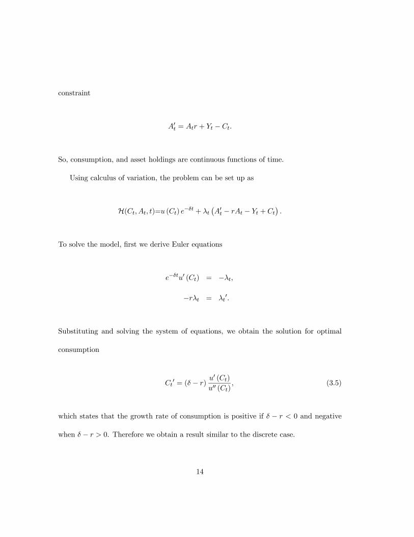
constraint
A0t = Atr + Yt − Ct.
So, consumption, and asset holdings are continuous functions of time.
Using calculus of variation, the problem can be set up as
H(Ct, At, t)=u (Ct) e−δt + λt¡A0t − rAt − Yt + Ct
¢.
To solve the model, first we derive Euler equations
e−δtu0 (Ct) = −λt,
−rλt = λt0.
Substituting and solving the system of equations, we obtain the solution for optimal
consumption
Ct0 = (δ − r) u
0 (Ct)
u00 (Ct), (3.5)
which states that the growth rate of consumption is positive if δ − r < 0 and negative
when δ − r > 0. Therefore we obtain a result similar to the discrete case.
14
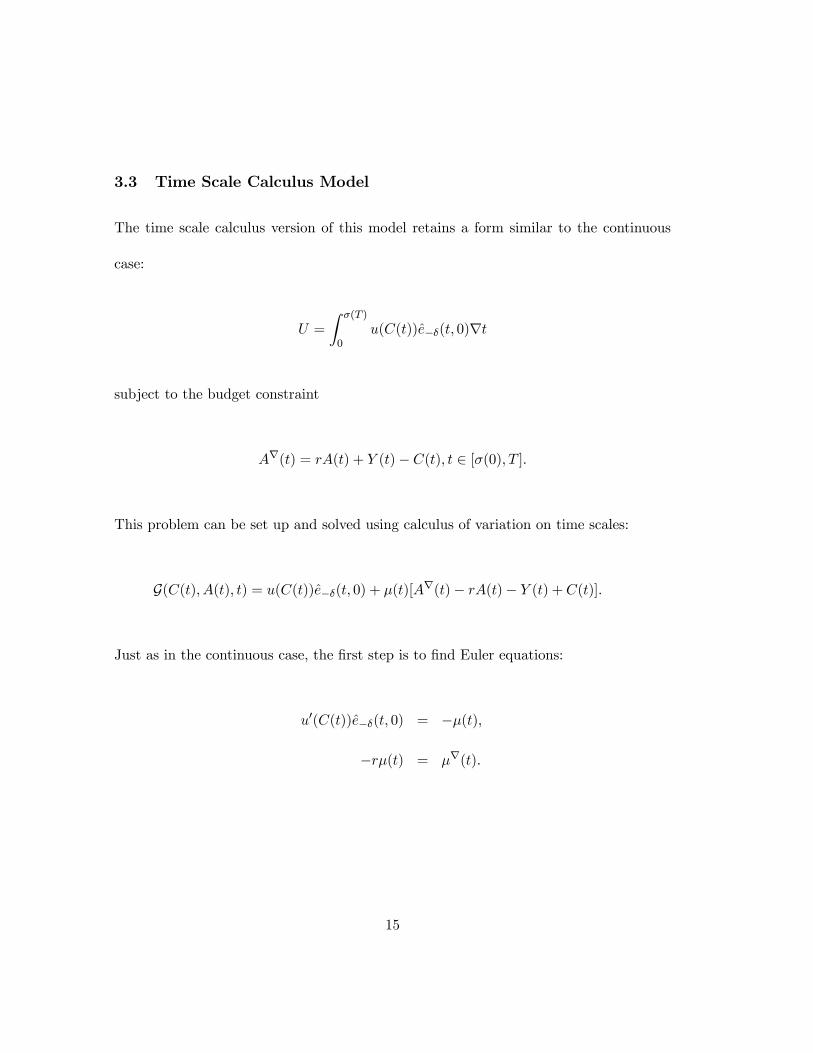
3.3 Time Scale Calculus Model
The time scale calculus version of this model retains a form similar to the continuous
case:
U =
Z σ(T )
0u(C(t))e−δ(t, 0)∇t
subject to the budget constraint
A∇(t) = rA(t) + Y (t)− C(t), t ∈ [σ(0), T ].
This problem can be set up and solved using calculus of variation on time scales:
G(C(t), A(t), t) = u(C(t))e−δ(t, 0) + μ(t)[A∇(t)− rA(t)− Y (t) +C(t)].
Just as in the continuous case, the first step is to find Euler equations:
u0(C(t))e−δ(t, 0) = −μ(t),
−rμ(t) = μ∇(t).
15

Substitution gives us the following dynamic equation:
e−δ(ρ(t), 0)[u0(C(t))]∇ = [δ − r]e−δ(t, 0)u0(C(t)).
Using a property of the ∇-exponential function [21], namely
e−δ(ρ(t), 0) = (1 + δν(t))e−δ(t, 0),
we obtain the following expression:
[u0(C(t))]∇ =δ − r
1 + δν(t)u0(C(t)). (3.6)
This equation conveys the same intuition as discrete and continuous models (equations
(3.3) and (3.5) respectively). The left-hand side of the equation is the ∇-derivative of
u0(C(t)). In the numerator of the right-hand side, ν(t) is the backward graininess function
ν(t) = t− ρ (t) . If consumption rises between t and t+ ν(t), then [u0(C(t))]∇ < 0. That
will be the case if δ− r < 0. Therefore, we obtain a result which covers both the discrete
and continuous cases.
16
3.4 Comparing Discrete, Continuous and Time Scale models
One of the main advantages of time scale models is that they unify discrete and contin-
uous models in a more general framework. Using definition the nabla-derivative and the
jump operators, it is straightforward to show that continuous and discrete models are
special cases of the time scale calculus model.
First, consider the discrete time model. When T = Z, the backward graininess
function becomes ν (t) = 1. The ∇-derivative of marginal utility becomes the difference
in marginal utilities between t − 1 and t: [u0(C(t))]∇ = u0(C(t)) − u0(C(t − 1)). Thus,
equation (3.6) can be written as
u0(C(t))− u0(C(t− 1)) = δ − r1 + δ
u0(C(t)). (3.7)
Rearranging equation (3.7) yields the same expressions as equation (3.3) . Thus, setting
T = Z converts the time scale calculus model into the discrete time model.
Next, consider the continuous model. When T = R, the backward graininess function
is ν (t) = 0 and the ∇-derivative of marginal utility is the conventional derivative with
respect to t: [u0(C(t))]∇ = d(u0(C(t)))dt . Substituting these two expressions into equation
(3.6) yields equation (3.5). Therefore, the continuous time model is a special case of the
time scale model.
Equation (3.6) also demonstrates another potential advantage of time scale calculus
17
models. If we parametrize the utility function, we can use equations (3.3), (3.5) and
(3.6) to solve for the growth rate of consumption. Discrete and continuous time models
would show that the growth rate of consumption for u(C) = lnC is constant because it
is determined by δ and r. The time scale calculus model implies that the growth rate of
consumption can change depending on the time scale because of ν (t). So, if consumption
data are collected at fixed intervals but the time scale is such that consumption occurs
with varying frequency, even if δ and r are constant, we would see fluctuations in the
observed growth rate of consumption.
Unification of the discrete and continuous models and ability to work with time-
varying frequencies are just a couple of many potential advantages time scale calculus
brings to economics. In the following section we discuss some other potential contribu-
tions of time scale calculus to economics.
4 Examples of Time Scales
In this section we solve the model presented in the previous section on several different
time scales and try to draw parallels with the discrete and continuous cases. We use time
scale version of Euler equation 3.6 to solve for the optimal consumption paths for different
time scales. The aim of these examples is to demonstrate how time scale calculus can
be used to study the problems in which timing of events is different from conventional
discrete (or, more precisely, evenly spaced over time) and continuous time models.
18

4.1 Example 1: T =Wh
This time scale is very similar to the conventional discrete model. As a matter of fact,
time scale techniques are not required to solve and analyze this model (e.g. see Obstfeld
and Rogoff 1998, pp 745-747). However, it is a good illustration of how time scale calculus
works.
For this time scale, the events take place at t, t+ h, t+ 2h, ... , t+ nh points in time,
so it is a slightly modified version of a discrete time model. Using the point classification
for time scales, all points are isolated and the jump function ν (t) = h. We can rewrite
the Euler equation 3.6 as
u0(C(t))− u0 (C (t− h))h
=δ − r1 + δh
u0(C(t)). (4.1)
If we employ a particular parametrization for the utility function, we can use this
equation to find out how income evolves over time. So, if we assume that utility function
is the standard constant relative risk aversion utility u (C (t)) = C1−θ
1−θ , then we can find
how consumption evolves over time:
C (t+ h) =
µ1 + hr
1 + hδ
¶ 1θ
C (t) (4.2)
If we know the present value of the income stream, we can consumption levels for each
period using the fact that the present value of consumption must equal present value of
19
0 4 6 8 9 10 11 15 17 19 20 21 220 4 6 8 9 10 11 15 17 19 20 21 22
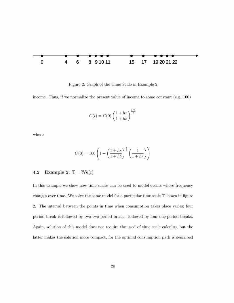
Figure 2: Graph of the Time Scale in Example 2
income. Thus, if we normalize the present value of income to some constant (e.g. 100)
C(t) = C(0)
µ1 + hr
1 + hδ
¶ t/hθ
where
C(0) = 100
Ã1−
µ1 + hr
1 + hδ
¶ 1θµ
1
1 + hr
¶!
4.2 Example 2: T =Wh(t)
In this example we show how time scales can be used to model events whose frequency
changes over time. We solve the same model for a particular time scale T shown in figure
2. The interval between the points in time when consumption takes place varies: four
period break is followed by two two-period breaks, followed by four one-period breaks.
Again, solution of this model does not require the used of time scale calculus, but the
latter makes the solution more compact, for the optimal consumption path is described
20
by the same equation (3.6)
[u0(C(t))]∇ =δ − r
1 + δν(t)u0(C(t)),
where ν(t) = {1, 2, 4} . We use the Euler equation to derive the path of consumption for
CRRA utility function as we did in the previous example. First, the present value of the
consumption path is
PV = C(0)∞Xi=1
¡aib2ic4i
¡1 + c−1 + c−2 + c−3 + c−4
¡1 + b−1 + b−2
¢¢¢,
where a =³(1+4r)1−θ
1+4δ
´ 1θ, b =
³(1+2r)1−θ
1+2δ
´ 1θ, c =
³(1+r)1−θ
1+δ
´ 1θ. This expression can be
approximated numerically for a set of parameters θ, δ and r. Once the present value of
consumption path is computed, we can solve recursively for consumption levels at each
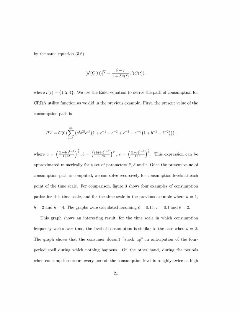
point of the time scale. For comparison, figure 3 shows four examples of consumption
paths: for this time scale, and for the time scale in the previous example where h = 1,
h = 2 and h = 4. The graphs were calculated assuming δ = 0.15, r = 0.1 and θ = 2.
This graph shows an interesting result: for the time scale in which consumption
frequency varies over time, the level of consumption is similar to the case when h = 2.
The graph shows that the consumer doesn’t ”stock up” in anticipation of the four-
period spell during which nothing happens. On the other hand, during the periods
when consumption occurs every period, the consumption level is roughly twice as high
21
1
6
11
16
21
26
31
36
0 2 4 6 8 10 12 14 16 18 20 22 24 26 28 30 32 34 36 38 40 42 44 46 48 50 52 54 56 58 60t
h=1
h=2
h=4
h-variable
Figure 3: Comparison of consumption paths on the h = 1, h = 2, h = 4 and time variabletime scales
22
0 1 2 30 1 2 3
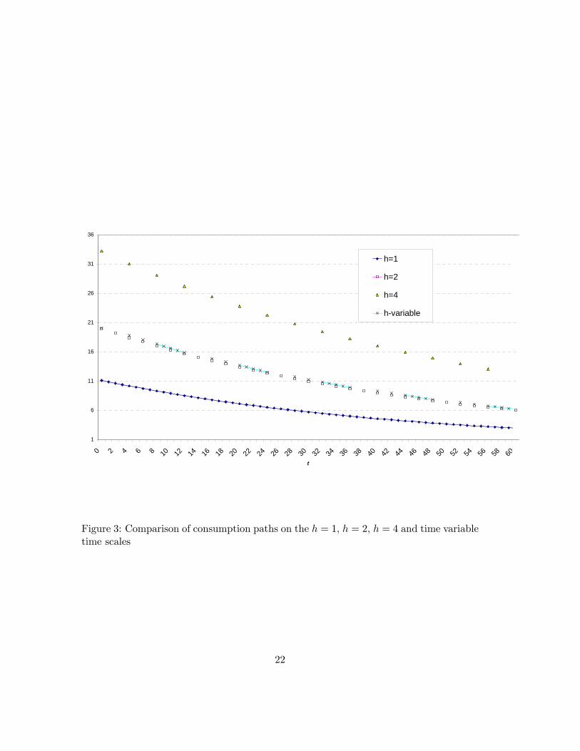
Figure 4: Graph of the P1,1 time scale
as it would be when h = 1. So it appears, that the determining factor of consumption
level is the average number of times consumption occurs per period. Because the average
number of consumption points is the same as when h = 2, the consumptions paths for the
h = 2 time scale and the variable time scale are similar. This is a fairly counterintuitive
implication because in reality we would expect consumers to reduce the consumption
when it occurs at higher frequency and increase with lower frequency. Most likely, this
result is due to additively-separable utility function.
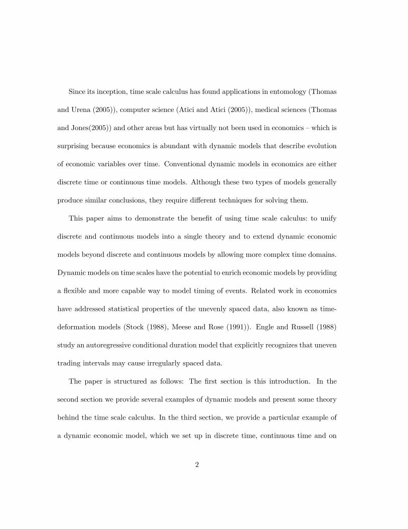
4.3 Example 3: T = P1,1
The time scale in this example can be described as evenly spaced intervals of real line:
P1,1 =∞Sk=0
[2k, 2k + 1] where k ∈ W. The graph of this time scale is shown in figure
4: Thus consumption occurs continuously for one period followed by a period without
consumption. Euler equation 3.6 during the consumption periods is the same as in
continuous time case (Eq. 3.5). Change in consumption between the end of the last
consumption period and beginning of the new consumption period can be described by
Euler equation for discrete case (Eq. 3.3). Once again, if assume CRRA utility, we can
23
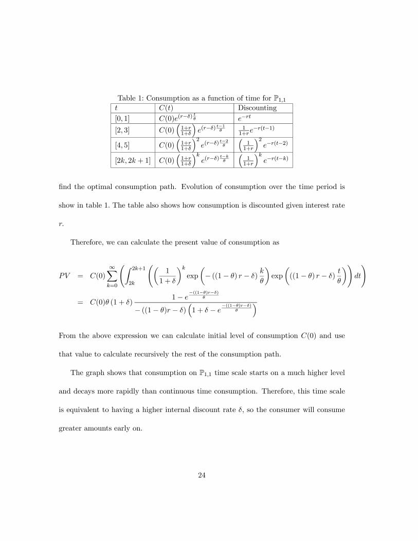
Table 1: Consumption as a function of time for P1,1t C(t) Discounting
[0, 1] C(0)e(r−δ)tθ e−rt
[2, 3] C(0)³1+r1+δ
´e(r−δ)
t−1θ
11+re
−r(t−1)
[4, 5] C(0)³1+r1+δ
´2e(r−δ)
t−2θ
³11+r
´2e−r(t−2)
[2k, 2k + 1] C(0)³1+r1+δ
´ke(r−δ)
t−kθ
³11+r
´ke−r(t−k)
find the optimal consumption path. Evolution of consumption over the time period is
show in table 1. The table also shows how consumption is discounted given interest rate
r.
Therefore, we can calculate the present value of consumption as
PV = C(0)∞Xk=0
ÃZ 2k+1
2k
õ1
1 + δ
¶kexp
µ− ((1− θ) r − δ)
k
θ
¶exp
µ((1− θ) r − δ)
t
θ
¶!dt
!
= C(0)θ (1 + δ)1− e
−((1−θ)r−δ)θ
− ((1− θ)r − δ)³1 + δ − e
−((1−θ)r−δ)θ
´From the above expression we can calculate initial level of consumption C(0) and use
that value to calculate recursively the rest of the consumption path.
The graph shows that consumption on P1,1 time scale starts on a much higher level
and decays more rapidly than continuous time consumption. Therefore, this time scale
is equivalent to having a higher internal discount rate δ, so the consumer will consume
greater amounts early on.
24

0
0.05
0.1
0.15
0.2
0.25
20 40 60 80 100t
Figure 5: Comparison of the continuous time and the P1,1 time scale consumption paths.
25
5 Conclusion
The main themes of time scale calculus are unification and extension: it aims to unify
existing differential and difference equation techniques into one set of techniques and
to expend dynamic models by studying more complex time scales. This paper provides
several examples of time scale models with the hope of attracting more economists to
time scale models by showing that this relatively simple technique offers rich modeling
capabilities.
References
[1] Agarwal, R. P., Bohner, M., Basic calculus on time scales and some of its applica-
tions, Results Math., 35(1-2),1999, 3-22.
[2] Agarwal, R. P., Bohner, M. and O’Regan, D., Time scale boundary value prob-
lems on infinite intervals J. Comput. Appl. Math., 141(1—2), 2002, 27-34. Special
Issue on ”Dynamic Equations on Time Scales”, edited by R.P. Agarwal, M. Bohner,
D.O’Regan.
[3] Aghion, P., Howitt, P., Endogenous Growth, MIT Press, 1997.
[4] Andersen, T. G., Bollerslev, T., Diebold, F. X., Vega, C., Micro Effects of Macro An-
nouncements: Real-Time Price Discovery in Foreign Exchange, American Economic
Review, 93(1), 2003, 38-62.
26
[5] Anderson, D. R., Solutions to second-order three-point problems on time scales, J.
Differ. Equs. and Appl., 8, 2002, 673-688.
[6] Atici, F. M., Guseinov, G. Sh. and Kaymakcalan, B., On Lyapunov inequality in
stability theory for Hill’s equation on time scales, J. Inequal. Appl., 5, 2000, 603-620.
[7] Atici, F. M., Eloe, P. W. and Kaymakcalan, B., The quasilinearization method for
boundary value problems on time scales, J. Mathematical Analysis and Applications,
276, 2002, 357-372.
[8] Atici, F. M. and Akin-Bohner, E., A quasilinearization approach for two point non-
linear boundary value problems on time scales, The Rocky Mountain Journal of
Mathematics, 35(1),2005, 19-46.
[9] Atici, F. M. and Biles, D. C., First order dynamic inclusions on time scales, J.
Mathematical Analysis and Applications, 292(1), 2004, 222-237.
[10] Atici, F. M. and Topal, S. G., Nonlinear three-point boundary value problems on
time scales, Dynamic Systems and Applications, 13, 2004, 327-337.
[11] Atici, F. M. and Topal, S. G., The generalized quasilinearization method and three-
point boundary value problems on time scales, Applied Math. Letters, 18(5), 2005,
577-585.
27

[12] Atici, F. M. and Guseinov, G. Sh., On Green’s functions and positive solutions for
boundary value problems on time scales, J. Comput. Appl. Math., 141, 2002, 75-99.
[13] Atici, F. M., Cabada, A., Chyan, C. J., Kaymakcalan, B., Nagumo type existence
results for second order nonlinear dynamic BVPs, Nonlinear Analysis, 60(2), 2004,
209-220.
[14] Atici, F. M. and Biles, D. C., First and second order dynamic equations with impulse,
Journal of Advances in Difference Equations,(2005) (to appear).
[15] Atici, F. M., Biles, D. C. and Lebedinsky, A., An Application of Time Scales to
Economics, submitted Computer and Mathematical Modelling
[16] Atici, F. M. and Atici, M., Master Theorem on Time Scales, in preparation.
[17] Barro, R., Sala-i-Martin, J., Economic Growth, 2nd edition, MIT Press, 2003.
[18] Benchohra, M., Henderson, J., Ntouyas, S. K. and Ouahabi, A., On first order
impulsive dynamic equations on time scales, J. Difference Equ. Appl., 10(6), 2004,
541—548.
[19] Benchohra, M., Ntouyas, S. K., Ouahabi, A., Existence results for second order
boundary value problem of impulsive dynamic equations on time scales, J. Math.
Anal. Appl., 296, 2004, 65-73.
28
[20] Bohner, M. and Peterson, A., Dynamic Equations on Time Scales, An Introduction
with Applications, Birkhauser, Boston, 2001.
[21] Bohner, M. and Peterson, A., Advances in Dynamic Equations on Time Scales,
Birkhauser, Boston, 2003.
[22] Bohner, M., Calculus of variations on time scales, Dynam. Systems Appl. 13(3-4),
2004, 339—349.
[23] Campbell J.Y., Lo A.W., MacKinlay A.C., The Econometrics of Financial Markets,
Princeton University Press, 1997.
[24] Choi, In, Effects of Data Aggregation on the Power of Tests for a Unit Root: A
Simulation Study, Economics Letters, 40(4), 1992, 397-401.
[25] Cochrane, J., Asset Pricing, Princeton University Press, Revised edition, 2005.
[26] Engle, R. F., The Econometrics of Ultra High Frequency Data, Econometrica, 68(1),
2000, 1-22.
[27] Engle R., Russell, J., Autoregressive conditional Duration: A new model for irreg-
ularly spaced transaction data, Econometrica, 66(5), 1998, 1127-1162.
[28] Eloe, P. W., The method of quasilinearization and dynamic equations on compact
measure chains, J. Comput. Appl. Math., 141, 2002, 159—167.
29

[29] Erbe , L. and Peterson, A., Green’s functions and comparison theorems for differen-
tial equations on measure chains, Dynam. Contin. Discrete Impuls. Systems, 6(1),
1999, 121—137.
[30] Garrett, T. Aggregated versus Disaggregated Data in Regression Analysis: Implica-
tions for Inference, Economics Letters, 81(1), 2003, 61-65.
[31] Hamilton, J.D., Time Series Analysis, Princeton University Press, 1994.
[32] Heaton, J., Lucas, D. J., Evaluating the effecs of incomplete markets on risk sharing
and asset pricing, The Journal of Political Economy, 104(3), 1996, 443-487.
[33] Henderson, J., Double solutions of impulsive dynamic boundary value problems on
a time scale, J. Difference Equ. Appl., 8, 2002, 345-356.
[34] Hilger, S., Ein Maßkettenkalkul mit Anwendung auf Zentrumsmannigfaltigkeiten.
Ph.D thesis, Universtat Wurzburg, 1988.
[35] Hilscher, R and Zeidan,V., Calculus of variations on time scales: weak local piecewise
C1rd solutions with variable endpoints, J. Math. Anal. Appl. 289(1), 2004, 143—166.
[36] Hwang, S., The Effects of Systematic Sampling and Temporal Aggregation on Dis-
crete Time Long Memory Processes and Their Finite Sample Properties, Economet-
ric Theory, 16(3),2000, 347-72.
30

[37] Kamionka, T. Simulated Maximum Likelihood Estimation in Transition Models,
Econometrics Journal, 1(1), 1998, 129-53.
[38] Ljungqvist, L and Sargent, T. J., Recursive Macroeconomic Theory, 2nd Edition
MIT Press, 2004.
[39] Meddahi, N., Renault E., Temporal Aggregation of Volatility Models, Journal of
Econometrics, 119(2), 2004, 355-79.
[40] Obstfeld, M. and Rogoff, K., Foundations of international Macroeconomics, MIT
1998.
[41] Romer, D., Advanced Macroeconomics, McGraw-Hill, 1996.
[42] Shen, C. H., Forecasting Macroeconomic Variables Using Data of Different Period-
icities, International Journal of Forecasting, 12(2), 1996, 269-82.
[43] Souza, L. R., Smith, J., Effects of Temporal Aggregation on Estimates and Forecasts
of Fractionally Integrated Processes: A Monte-Carlo Study, International Journal
of Forecasting, 20(3), 2004, 487-502.
[44] Stock, J., Estimating Continuos-Time Processes Subject to Time Deformation: An
Application to Post-War U.S. GNP. Journal of the American Statistical Association,
83(401), 1988, 77-85
[45] Stokey, N. and Lucas, R., Recursive Methods in Economic Dynamics, Harvard, 1989.
31

[46] Thelmer, C. I., Asset Pricing Puzzles and incomplete markets, The Journal of Fi-
nance, 48(5), 1993, 1803-1832.
[47] Thomas, D. and Jones M. A., Mathematical Model for Debriding a Wound, Math
and Computer Modelling, (to appear).
[48] Thomas, D. and Urena, B., A Mathematical Model Describing the Evolution of
Encephalitis in New York City, Mathematical and Computer Modelling,(to appear).
32