Embed Size (px)
Citation preview
Examples of Nonclassical Feedback Control Problems
Alberto Bressan and Deling Wei
Department of Mathematics, Penn State University
University Park, Pa. 16802, U.S.A.
e-mails: [email protected] , [email protected]
December 6, 2011
Abstract
We consider a control system with “nonclassical” dynamics: x = f(t, x, u,Dxu), wherethe right hand side depends also on the first order partial derivatives of the feedbackcontrol function. Given a probability distribution on the initial data, we seek a feedbacku = u(t, x) which minimizes the expected value of a cost functional. Various relaxedformulations of this problem are introduced. In particular, three specific examples arestudied, showing the equivalence or non-equivalence of these approximations.
1 Introduction
Consider a controlled system whose state x ∈ IRn evolves according to
x = f(t, x, u,Du) . (1.1)
Here u = u(t, x) is a feedback control, taking values in a set U ⊆ IRm, while the upperdot denotes a derivative w.r.t. time. The dependence of the right hand side of (1.1) on theJacobian matrix Du = (∂ui/∂xj) makes the problem “nonclassical”. Control systems withthis generalized dynamics arise naturally in connection with closed-loop Stackelberg solutionsto differential games [5, 6, 8].
As remarked in [8], it is useful to compare (1.1) with the relaxed system
x = f(t, x, u, v) , (1.2)
where u ∈ IRm, v ∈ IRm×n are now regarded as independent controls. Clearly, every solutionof (1.1) yields a solution of (1.2), simply by choosing v = Du. On the other hand, given aninitial data
x(0) = x0 , (1.3)
let t 7→ x∗(t) be the solution of the Cauchy problem (1.2)-(1.3) corresponding to the open-loopmeasurable controls u(t), v(t). If we choose
u∗(t, x) = u(t) + v(t) · (x− x∗(t)) (1.4)
1
for all x in a neighborhood of x∗(t), then x∗ satisfies also the original equation (1.1).
Given a cost functional such as
J.=
∫ T
0L(
t, x(t), u(t, x(t)))
dt , (1.5)
for a fixed initial condition (1.3) the infimum of the cost over all admissible controls is thus thesame for trajectories of (1.1) or (1.2). The main difficulty in the study of this minimizationproblem lies in the fact that the control v can be arbitrarily large and comes at zero cost.Therefore, optimal trajectories may well have impulsive character. For optimization problemswith impulsive controls we refer to [7, 10, 11].
Aim of the present paper is to understand what happens in the case where the initial data isnot assigned in advance, and one seeks a feedback u = u(t, x) that is optimal in connectionwith a whole collection of possible initial data. Motivated by problems related to differentialgames [5, 6, 8], we consider a system whose state is described by a pair of scalar variables(x, ξ) ∈ IR × IR. For simplicity, we also assume that the control variable u(t) ∈ IR is one-dimensional. Let the system evolve in time according to the ODEs
x = f(t, x, ξ, u) ,
ξ = g(t, x, ξ, u, ux) ,
(1.6)
where f, g are Lipschitz continuous functions of their arguments. We assume that the initialdata for the variable x is distributed according to a probability distribution µ on IR, while ξis determined by a constraint of the form
ξ(0) = h(x(0)) . (1.7)
Here h : IR 7→ IR is some continuous function. A feedback control u = u(t, x) is sought, inorder to minimize the cost functional
J(u, µ).= Eµ
[∫ T
0L(
t, x(t), ξ(t), u(t, x(t)))
dt
]
. (1.8)
Here Eµ denotes the conditional expectation w.r.t. the probability distribution µ on the setof initial data.
In general, a optimal feedback may not exist, within the class of C2 functions. Indeed, it isquite possible that the optimal control will be discontinuous w.r.t. the space variable x, oreven measure-valued. To bypass all difficulties stemming from the possible lack of regularity,we consider the family U of all C2 functions u : [0, T ] × IR 7→ IR. For each feedback controlu ∈ U the equation (1.6) uniquely determines a flow on IR2. We denote by
t 7→(
x(t)ξ(t)
)
= Ψut
(
xξ
)
the solution of the Cauchy problem
d
dt
(
x(t)ξ(t)
)
=
f(
t, x(t), ξ(t), u(t, x(t)))
g(
t, x(t), ξ(t), u(t, x(t)), ux(t, x(t)))
, (1.9)
2
with initial data(
x(0)ξ(0)
)
=
(
xξ
)
=
(
xh(x)
)
. (1.10)
Here x ∈ IR is a random variable, distributed according to the probability measure µ. Letµ(t) be the corresponding probability distribution at time t, defined as the push-forward of µthrough the flow Ψu
t . This means
µ(t)(Ψut (A)) = µ(A)
for every Borel set A ⊂ IR2. The cost functional in (1.8) can be equivalently written as
J(u, µ) =
∫ T
0Eµ(t)
L(
t, x, ξ, u(t, x))
dt , (1.11)
where Eµ(t)denotes expectation w.r.t. the probability distribution µ(t). We then consider
Problem 1. DetermineJ(µ)
.= inf
u∈UJ(u, µ). (1.12)
Describe a sequence of feedback controls (un)n≥1 achieving the infimum in (1.12).
As it will be shown by some examples, the infimum in (1.12) may not be stable w.r.t. pertur-bations of the probability distribution µ. A related question is to determine the value
Jw(µ).= lim inf
d(µ,µ)→0infu∈U
J(u, µ), (1.13)
where
d(µ, µ) = sup
{∣
∣
∣
∣
∫
ϕdµ −∫
ϕdµ
∣
∣
∣
∣
; ϕ ∈ C1 , |∇ϕ| ≤ 1
}
is the Kantorovich-Wasserstein distance between two probability measures. One can think ofJw as the lower semicontinuous regularization of J w.r.t. the topology of weak convergence ofmeasures.
In the case where µ is absolutely continuous with density φ w.r.t. Lebesgue measure, it is alsomeaningful to consider
Js(µ).= lim inf
‖φ−φ‖L1→0
infu∈U
J(u, µ), (1.14)
where µ is a probability measure having density φ. In other words, Js is the lower semicon-tinuous regularization of J w.r.t. a strong topology, corresponding to L1 convergence of thedensities.
As it will be shown by specific examples, the three values in (1.12)-(1.14) may well be different.In addition, by replacing ux with an independent control function v, from (1.9) one obtainsthe relaxed system
d
dt
(
x(t)ξ(t)
)
=
f(
t, x(t), ξ(t), u(t, x(t)))
g(
t, x(t), ξ(t), u(t, x(t)), v(t, x(t)))
. (1.15)
We shall denote by J (µ, u, v) be the corresponding cost (1.8), with dynamics given at (1.15).
3
Remark 1. In general, the optimal control u = u(t, x) which minimizes the expected cost(1.8) subject to the dynamics (1.9) will strongly depend on the probability distribution µ onthe initial data. On the other hand, since the dynamics (1.15) does not involve derivatives ofthe control functions u, v, the optimal value can be achieved pointwise for each initial datax(0), ξ(0). In this case, the same pair of feedback controls (u∗, v∗) can be optimal for everyprobability distribution µ on the initial data.
We now introduce the set V of all C2 functions v : [0, T ]× IR 7→ IR, and consider
Problem 2: Determine the optimal value for the relaxed problem
Jrelax(µ).= inf
(u,v)∈U×VJ (u, v, µ). (1.16)
Describe a sequence of feedback controls (un, vn)n≥1 achieving the infimum in (1.16).
From the definitions, it is immediately clear that
Jrelax(µ) ≤ J(µ) , Jw(µ) ≤ Js(µ) ≤ J(µ) . (1.17)
In this paper we analyze three specific examples. showing the differences between the originaland relaxed formulations, and the possible obstructions encountered in the approximation ofsolutions (1.15) with solutions of (1.9). Motivated by these examples, general results on theequivalence between the various values in (1.17) will be proved in the forthcoming paper [2].
The underlying motivation for the present analysis comes from the theory of Stackelberg so-lutions in closed-loop form, for differential games. In one space dimension, this leads to aproblem of the form (1.6), where x is the state of the system, u = u(t, x) is the feedbackcontrol implemented by the leader, and ξ is the adjoint variable in the optimality equation de-termining the strategy of the follower. For a differential game, it is natural to put a probabilitydistribution on the state x at the initial time t = 0, and a constraint of the type
ξ(T ) = h(x(T ))
on the adjoint variable at the terminal time T . The present research, dealing with the Cauchyproblem where all data are given at time t = 0, is intended to be an intermediate steptoward the understanding of this boundary value problem, more relevant for game-theoreticapplications.
2 A case of shrinking funnels
Example 1. Consider the optimization problem
minimize: J(u) = Eµ
[∫ T
0[x2(t) + ξ2(t) + u2(t)] dt
]
. (2.1)
for the system with dynamics{
x = u ,
ξ = ξux .(2.2)
4
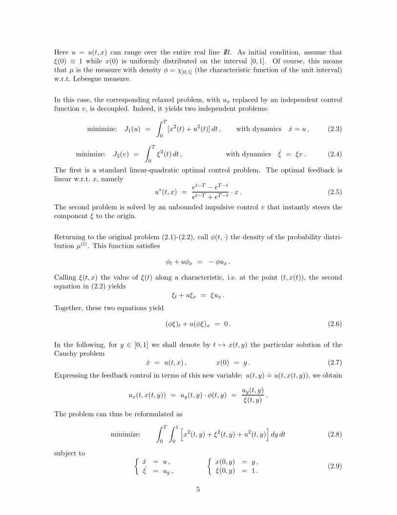
Here u = u(t, x) can range over the entire real line IR. As initial condition, assume thatξ(0) ≡ 1 while x(0) is uniformly distributed on the interval [0, 1]. Of course, this meansthat µ is the measure with density φ = χ[0,1] (the characteristic function of the unit interval)w.r.t. Lebesgue measure.
In this case, the corresponding relaxed problem, with ux replaced by an independent controlfunction v, is decoupled. Indeed, it yields two independent problems:
minimize: J1(u) =
∫ T
0[x2(t) + u2(t)] dt , with dynamics x = u , (2.3)
minimize: J2(v) =
∫ T
0ξ2(t) dt , with dynamics ξ = ξv . (2.4)
The first is a standard linear-quadratic optimal control problem. The optimal feedback islinear w.r.t. x, namely
u∗(t, x) =et−T − eT−t
et−T + eT−t· x . (2.5)
The second problem is solved by an unbounded impulsive control v that instantly steers thecomponent ξ to the origin.
Returning to the original problem (2.1)-(2.2), call φ(t, ·) the density of the probability distri-bution µ(t). This function satisfies
φt + uφx = − φux .
Calling ξ(t, x) the value of ξ(t) along a characteristic, i.e. at the point (t, x(t)), the secondequation in (2.2) yields
ξt + uξx = ξux .
Together, these two equations yield
(φξ)t + u(φξ)x = 0 . (2.6)
In the following, for y ∈ [0, 1] we shall denote by t 7→ x(t, y) the particular solution of theCauchy problem
x = u(t, x) , x(0) = y . (2.7)
Expressing the feedback control in terms of this new variable: u(t, y).= u(t, x(t, y)), we obtain
ux(t, x(t, y)) = uy(t, y) · φ(t, y) =uy(t, y)
ξ(t, y).
The problem can thus be reformulated as
minimize:
∫ T
0
∫ 1
0
[
x2(t, y) + ξ2(t, y) + u2(t, y)]
dy dt (2.8)
subject to{
x = u ,
ξ = uy ,
{
x(0, y) = y ,ξ(0, y) = 1 .
(2.9)
5

Since the evolution equation does not depend explicitly on x, ξ, the adjoint equations are
λ1 = − ∂L/∂x = − 2x ,
λ2 = − ∂L/∂ξ = − 2ξ ,
λ1(T, y) = 0 ,
λ2(T, y) = 0 .(2.10)
Hence
λ1(t, y) =
∫ T
t2x(τ, y) dτ , λ2(t, y) =
∫ T
t2 ξ(τ, y) dτ . (2.11)
The maximality condition yields
u(t, ·) = argminω(·)
∫ 1
0
[
λ1(t, y)ω(y) + λ2(t, y)ωy(y) + ω2(y)]
dy . (2.12)
0
1
x
tT
x
t
x
t
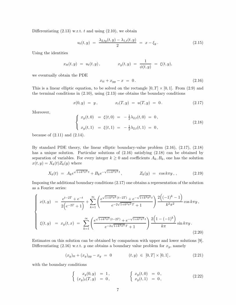
Figure 1: Left: the optimal trajectories for the standard linear-quadratic optimization problem withdynamics (2.9) and cost (2.3) independent of ξ. Center: the presence of a cost depending on ξ rendersmore profitable a control where ux is large and negative. Hence the optimal solution, obtained bysolving (2.16), should be supported on a smaller interval. Right: if we allow small gaps in the supportof the probability distribution µ on the initial data, then the minimum cost becomes arbitrarily closeto the minimum cost for relaxed problem (2.3)-(2.4).
Assume that, for a fixed time t, the function u = u(t, y) provides the minimum in (2.12).Then, for every smooth function ϕ : [0, 1] 7→ IR, setting u(ε)(y) = u(t, y) + εϕ(y) one shouldhave
0 =d
dε
∫ 1
0
[
λ1(t, y)u(ε)(y) + λ2(t, y)u
(ε)y (y) + (u(ε))2(y)
]
dy
∣
∣
∣
∣
ε=0
=
∫ 1
0
[
λ1(t, y)ϕ(y) + λ2(t, y)ϕy(y) + 2u(t, y)ϕ(y)]
dy
=
∫ 1
0
[
λ1(t, y)− λ2,y(t, y) + 2u(t, y)]
ϕ(y) dy + λ2(t, 1)ϕ(1) − λ2(t, 0)ϕ(0) .
Since the function ϕ can be arbitrary, this yields the Euler-Lagrange equations
u(t, y) =−λ1(t, y) + λ2,y(t, y)
2. (2.13)
together with the boundary conditions
λ2(t, 0) = λ2(t, 1) = 0 . (2.14)
6
Differentiating (2.13) w.r.t. t and using (2.10), we obtain
ut(t, y) =λ2,ty(t, y)− λ1,t(t, y)
2= x− ξy . (2.15)
Using the identities
xtt(t, y) = ut(t, y) , xy(t, y) =1
φ(t, y)= ξ(t, y),
we eventually obtain the PDExtt + xyy − x = 0 . (2.16)
This is a linear elliptic equation, to be solved on the rectangle [0, T ] × [0, 1]. From (2.9) andthe terminal conditions in (2.10), using (2.13) one obtains the boundary conditions
x(0, y) = y , xt(T, y) = u(T, y) = 0 . (2.17)
Moreover,
xy(t, 0) = ξ(t, 0) = − 12λ2,t(t, 0) = 0 ,
xy(t, 1) = ξ(t, 1) = − 12λ2,t(t, 1) = 0 ,
(2.18)
because of (2.11) and (2.14).
By standard PDE theory, the linear elliptic boundary-value problem (2.16), (2.17), (2.18)has a unique solution. Particular solutions of (2.16) satisfying (2.18) can be obtained byseparation of variables. For every integer k ≥ 0 and coefficients Ak, Bk, one has the solutionx(t, y) = Xk(t)Zk(y) where
Xk(t) = Ake√1+k2π2 t +Bke
−√1+k2π2 t , Zk(y) = cos kπy , , (2.19)
Imposing the additional boundary conditions (2.17) one obtains a representation of the solutionas a Fourier series:
x(t, y) =et−2T + e−t
2(
e−2T + 1) +
∞∑
k=1
(
e√1+k2π2 (t−2T ) + e−
√1+k2π2 t
e−2√1+k2π2 T + 1
)
2(
(−1)k − 1)
k2π2cos kπy ,
ξ(t, y) = xy(t, x) =
∞∑
k=1
(
e√1+k2π2 (t−2T ) + e−
√1+k2π2 t
e−2√1+k2π2 T + 1
)
2(
1− (−1)k)
kπsin kπy .
(2.20)
Estimates on this solution can be obtained by comparison with upper and lower solutions [9].Differentiating (2.16) w.r.t. y one obtains a boundary value problem for xy, namely
(xy)tt + (xy)yy − xy = 0 (t, y) ∈ [0, T ]× [0, 1] , (2.21)
with the boundary conditions
{
xy(0, y) = 1 ,(xy)t(T, y) = 0 ,
{
xy(t, 0) = 0 ,xy(t, 1) = 0 ,
(2.22)
7
A standard comparison argument here yields the lower bound
xy(t, y) ≥ 0 for all t, y .
One can also consider the above problem on the half line, for t ∈ [0, +∞[ . In this case, (2.20)reduces to
x(t, y) =e−t
2+
∞∑
k=1
e−√1+k2π2 t ·
2(
(−1)k − 1)
k2π2cos kπy . (2.23)
As t → ∞, this solution approaches zero. Indeed,
‖x(t, ·)‖L∞([0,1]) → 0 , ‖ξ(t, ·)‖L∞([0,1]) → 0 , ‖u(t, ·)‖L∞([0,1]) → 0 . (2.24)
We now study what happens if we allow arbitrarily small gaps in the support of the initialprobability distribution µ. For any n ≥ 2, let µn be the probability distribution with density
φn(x) =
n
n− 1if x ∈ [ai, bi]
.=
[
i− 1
n,
i
n− 1
n2
]
, for some i = 1, . . . , n,
0 otherwise.(2.25)
Clearly, limn→∞ ‖φn − φ‖L1 = 0. We claim that, as n → ∞, the costs of the correspondingoptimal solutions approach the minimum cost for (2.3). To prove this, consider any of theabove intervals [ai, bi] ⊂ [0, 1]. Let xi(t, y) be the solution of the linear elliptic boundary valueproblem
xtt + xyy − x = 0 (t, y) ∈ [0, T ]× [ai, bi] , (2.26)
with boundary conditions
{
x(0, y) = y ,xt(T, y) = 0 ,
{
xy(t, ai) = 0 ,xy(t, bi) = 0 .
(2.27)
The solution to this boundary value problem can again be expressed as a Fourier series:
xi(t, y) =
(
et−2T + e−t
e−2T + 1
)
bi + ai2
+
∞∑
k=1
(
eλk (t−2T ) + e−λk t
e−2λk T + 1
)
2(
(−1)k − 1)
(bi − ai)
k2π2cos
kπ(y − ai)
bi − ai,
(2.28)where
λk =
√
1 +k2π2
(bi − ai)2≥ 1 .
In connection with the intervals [ai, bi] defined at (2.25), for i = 1, . . . , n consider the funnels
Γi.={
(t, x) ; t ∈ [0, T ] , x = xi(t, y) for some y ∈ [ai, bi]}
. (2.29)
8
We claim that these funnels are pairwise disjoint. Indeed, consider the function
z(t, y) =et−2T + e−t
e−2T + 1y (2.30)
where t 7→ z(t, y) is determined as the unique solution to the two-point boundary value problem
z(t)− z(t) = 0 for t ∈ [0, T ] , z(0) = y , z(T ) = 0 . (2.31)
Then zy provides a solution to the elliptic boundary value problem
wtt + wyy − w = 0 (t, y) ∈ [0, T ]× [ai, bi] , (2.32)
with boundary conditions
{
w(0, y) = 1 ,wt(T, y) = 0 ,
w(t, ai) = w(t, bi) =et−2T + e−t
e−2T + 1. (2.33)
On the other hand, the partial derivative xi,y provides a solution to the same equation (2.32),but with boundary conditions
{
w(0, y) = 1 ,wt(T, y) = 0 ,
w(t, ai) = (t, bi) = 0 . (2.34)
By comparison, we obtain
xy(t, y) ≤ zy(t, y) for all (t, y) ∈ [0, T ] × [ai, bi] . (2.35)
When y = (ai + bi)/2, from (2.28) it follows xi(t, y) = z(t, y) for all t ∈ [0, T ]. Since theestimates (2.35) hold for every i = 1, . . . , n, we conclude
xi−1(t, bi−1) ≤ z(t, bi−1) < z(t, ai) ≤ xi(t, ai),
proving that the funnels Γ1, . . . ,Γn remain disjoint.
We can now define a feedback control un by setting
un(t, x) = xi,t(t, y) if (t, x) ∈ Γi for some i ∈ {1 . . . , n} , (2.36)
and extending un in a smooth way to the entire domain [0, T ] × IR.
Proposition 1. The above construction yields
limn→∞
J(µn, un) = Jrelax(µ). (2.37)
Therefore, for this example one has Js(µ) = Jrelax(µ).
Proof. Writing the Euler-Lagrange equations for (2.3) and observing that the infimum costfor (2.4) is zero, we compute
Jrelax(µ) =
∫ 1
0
∫ T
0
(
z2(t, y) + z2t (t, y))
dt dy , (2.38)
9
where z is the function in (2.30). On the other hand,
J(µn, un) =n
n− 1
n∑
i=1
∫ bi
ai
∫ T
0
(
x2i (t, y) + x2i,t(t, y) + x2i,y(t, y))
dtdy , (2.39)
where, for y ∈ [ai, bi], the quantity xi(t, y) is given by (2.28). We observe that each functionxi provides the global minimizer to the variational problem
minimize: Ji(w).=
∫ bi
ai
∫ T
0
(
w2(t, y) + w2t (t, y) + w2
y(t, y))
dt dy (2.40)
among all functions w ∈ W 1,2([0, T ]× [ai, bi]) such that
w(0, y) = y for all y ∈ [ai, bi] . (2.41)
Consider the functions wi defined as follows. For y ∈ [ai, bi], let
wi(t, y).=
nt z( 1
n,ai + bi
2
)
+ (1− nt) y , if t ∈ [0, n−1] ,
z(
t,ai + bi
2
)
, if t ∈ [n−1, T ] .
(2.42)
For every n ≥ 1 and i ∈ {1, . . . , n}, it is easy to check that these functions satisfy the uniformbounds
wi(t, y) ∈ [0, 1] , wi,y(t, y) ∈ [0, 1] , |wi,t(t, y)| ≤ M , (2.43)
for some uniform constant M . Hence the following estimates hold:
∫ bi
ai
∫ T
0w2i,y(t, y) dt dy ≤
∫ bi
ai
∫ 1/n
0dt dy =
bi − ain
, (2.44)
∫ bi
ai
∫ 1/n
0
(
w2i (t, y) + w2
i,t(t, y))
dt dy ≤ (1 +M2)(bi − ai)
n. (2.45)
Using the above inequalities and recalling that∑n
i=1(bi − ai) = (n − 1)/n, since each xi :[0, T ]× [ai, bi] 7→ IR provides a global minimizer, we obtain
J(µn, un) ≤ n
n− 1
n∑
i=1
∫ bi
ai
∫ T
0
(
w2i (t, y) + w2
i,t(t, y) + w2i,y(t, y)
)
dt dy
≤ n
n− 1
n∑
i=1
(2 +M2)(bi − ai)
n
+n
n− 1
n∑
i=1
(bi − ai)
∫ T
1/n
(
z2(
t,ai + bi
2
)
+ z2t
(
t,ai + bi
2
)
)
dt
≤ (2 +M2)
n+
n∑
i=1
(ai+1 − ai)
∫ T
0
(
z2(
t,ai + bi
2
)
+ z2t
(
t,ai + bi
2
)
)
dt
.= An +Bn .
(2.46)
10
Letting n → ∞, we clearly have An → 0. On the other hand, Bn is an approximate Riemannsum for the integral (2.38). Hence limn→∞Bn = Jrelax(µ). From (2.46) it follows
lim infn→∞
J(µn , un) ≤ Jrelax(µ) ,
The converse inequality is clear.
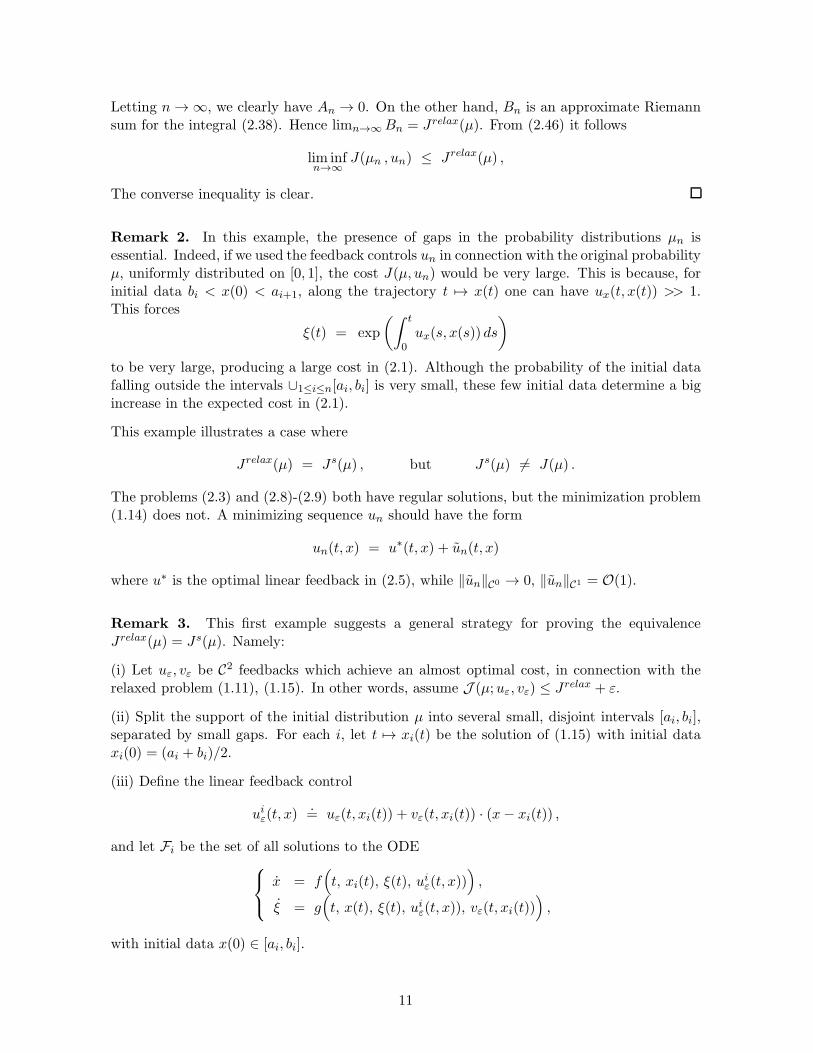
Remark 2. In this example, the presence of gaps in the probability distributions µn isessential. Indeed, if we used the feedback controls un in connection with the original probabilityµ, uniformly distributed on [0, 1], the cost J(µ, un) would be very large. This is because, forinitial data bi < x(0) < ai+1, along the trajectory t 7→ x(t) one can have ux(t, x(t)) >> 1.This forces
ξ(t) = exp
(∫ t
0ux(s, x(s)) ds
)
to be very large, producing a large cost in (2.1). Although the probability of the initial datafalling outside the intervals ∪1≤i≤n[ai, bi] is very small, these few initial data determine a bigincrease in the expected cost in (2.1).
This example illustrates a case where
Jrelax(µ) = Js(µ) , but Js(µ) 6= J(µ) .
The problems (2.3) and (2.8)-(2.9) both have regular solutions, but the minimization problem(1.14) does not. A minimizing sequence un should have the form
un(t, x) = u∗(t, x) + un(t, x)
where u∗ is the optimal linear feedback in (2.5), while ‖un‖C0 → 0, ‖un‖C1 = O(1).
Remark 3. This first example suggests a general strategy for proving the equivalenceJrelax(µ) = Js(µ). Namely:
(i) Let uε, vε be C2 feedbacks which achieve an almost optimal cost, in connection with therelaxed problem (1.11), (1.15). In other words, assume J (µ;uε, vε) ≤ Jrelax + ε.
(ii) Split the support of the initial distribution µ into several small, disjoint intervals [ai, bi],separated by small gaps. For each i, let t 7→ xi(t) be the solution of (1.15) with initial dataxi(0) = (ai + bi)/2.
(iii) Define the linear feedback control
uiε(t, x).= uε(t, xi(t)) + vε(t, xi(t)) · (x− xi(t)) ,
and let Fi be the set of all solutions to the ODE
x = f(
t, xi(t), ξ(t), uiε(t, x))
)
,
ξ = g(
t, x(t), ξ(t), uiε(t, x)), vε(t, xi(t)))
,
with initial data x(0) ∈ [ai, bi].
11
(iv) If the funnels
Γi.={
(t, x(t)) ; t ∈ [0, T ], x(·) ∈ Fi
}
, i = 1, . . . , n ,
do not overlap, then one can define a new feedback by setting
u(t, x).= uiε(t, x) if (t, x) ∈ Γi , (2.47)
and extending u in a smooth way on IR2 \ ∪iΓi. By choosing the intervals [ai, bi] sufficientlysmall, the cost provided by this feedback control u∗ can be rendered arbitrarily close toJ(µ, uε, vε).
Here the fact that the funnels Γi remain disjoint is essential. In the next section we look at acase where this property fails, and the two infimum costs Jrelax and Js do not coincide.
3 A case of expanding funnels
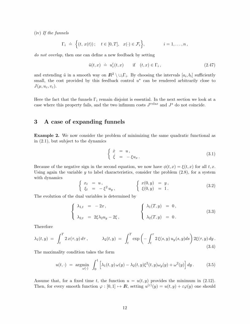
Example 2. We now consider the problem of minimizing the same quadratic functional asin (2.1), but subject to the dynamics
{
x = u ,
ξ = − ξux .(3.1)
Because of the negative sign in the second equation, we now have φ(t, x) = ξ(t, x) for all t, x.Using again the variable y to label characteristics, consider the problem (2.8), for a systemwith dynamics
{
xt = u ,ξt = − ξ2 uy ,
{
x(0, y) = y ,ξ(0, y) = 1 .
(3.2)
The evolution of the dual variables is determined by
λ1,t = − 2x ,
λ2,t = 2ξλ2uy − 2ξ ,
λ1(T, y) = 0 ,
λ2(T, y) = 0 .(3.3)
Therefore
λ1(t, y) =
∫ T
t2x(τ, y) dτ , λ2(t, y) =
∫ T
texp
(
−∫ τ
t2 ξ(s, y)uy(s, y)ds
)
2ξ(τ, y) dy .
(3.4)The maximality condition takes the form
u(t, ·) = argminω(·)
∫ 1
0
[
λ1(t, y)ω(y)− λ2(t, y)ξ2(t, y)ωy(y) + ω2(y)
]
dy . (3.5)
Assume that, for a fixed time t, the function u = u(t, y) provides the minimum in (2.12).Then, for every smooth function ϕ : [0, 1] 7→ IR, setting u(ε)(y) = u(t, y) + εϕ(y) one should
12
have
0 =d
dε
∫ 1
0
[
λ1(t, y)u(ε)(y)− λ2(t, y)ξ
2(t, y)u(ε)y (y) + (u(ε))2(y)]
dy
∣
∣
∣
∣
ε=0
=
∫ 1
0
[
λ1(t, y)ϕ(y) − λ2(t, y)ξ2(t, y)ϕy(y) + 2u(t, y)ϕ(y)
]
dy
=
∫ 1
0
[
λ1(t, y) + (λ2ξ2)y(t, y) + 2u(t, y)
]
ϕ(y) dy + λ2(t, 1)ξ2(t, 1)ϕ(1) − λ2(t, 0)ξ
2(t, 0)ϕ(0) .
Since the function ϕ can be arbitrary, this yields the Euler-Lagrange equations
u(t, y) = − λ1(t, y) + (λ2ξ2)y(t, y)
2. (3.6)
together with the boundary conditions
(λ2ξ2)(t, 0) = (λ2ξ
2)(t, 1) = 0 . (3.7)
Observe that (3.2) and (3.3) yield
(λ2ξ2)t = (2ξλ2uy − 2ξ)ξ2 − λ2ξ
2uy = − 2ξ3. (3.8)
Differentiating both sides of (3.6) w.r.t. t and using (3.8) one obtains
ut(t, y) = − λ1,t(t, y) + (λ2ξ2)t,y(t, y)
2= x+ (ξ3)y . (3.9)
Using the identities
xtt(t, y) = ut(t, y) , xy(t, y) =1
φ(t, y)=
1
ξ(t, y), (3.10)
we thus recover the PDE
xtt +3xyy(xy)4
− x = 0 . (3.11)
This is a nonlinear elliptic equation, to be solved on the rectangle [0, T ] × [0, 1]. From (3.2)and the terminal conditions in (3.3), using (3.6) one obtains the boundary conditions
x(0, y) = y , xt(T, y) = u(T, y) = 0 . (3.12)
Moreover,
xy(t, 0) =1
ξ(t, 0)= +∞ ,
xy(t, 1) =1
ξ(t, y)= +∞ ,
(3.13)
because 0 = (λξ2)t(t, 0) = −2ξ3(t, 0), 0 = (λξ2)t(t, 1) = −2ξ3(t, 1).
In contrast with the optimal solution in Example 1, letting T → ∞ the optimal trajectoriesdo not converge to zero. Rather than (2.24), we expect that the solution x(t, y), ξ(t, y) will
13
1
tT T0
x
T
x
0 0
1x1
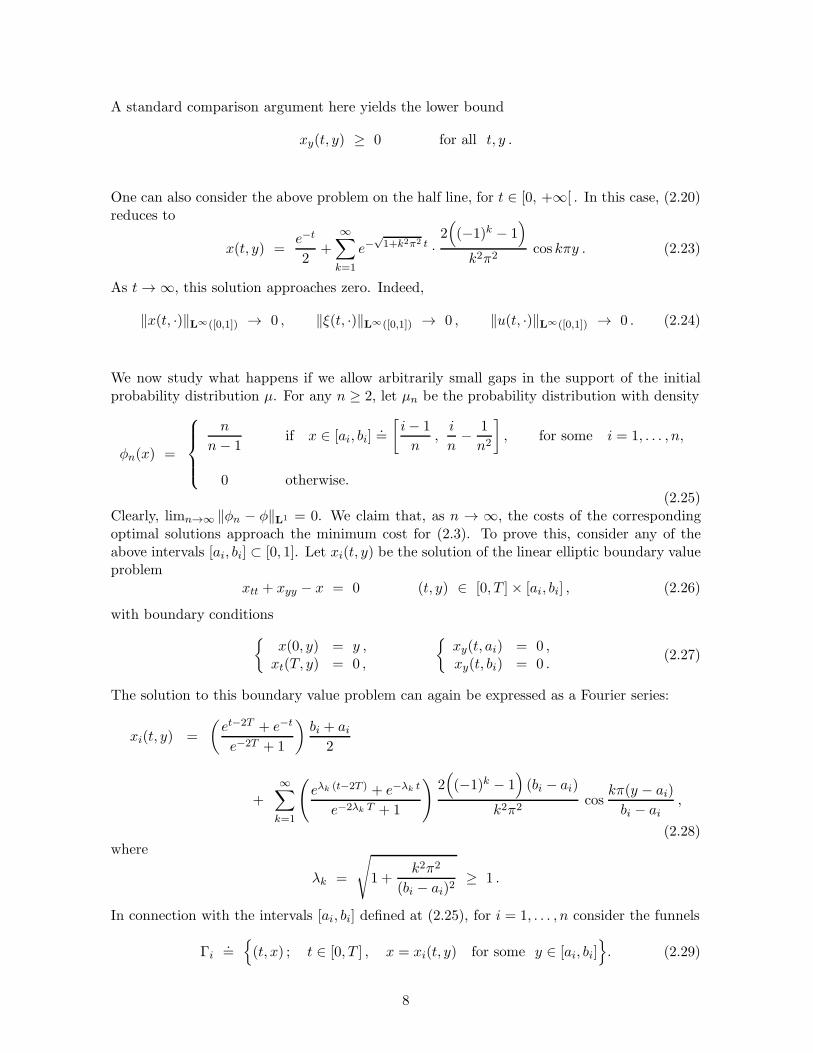
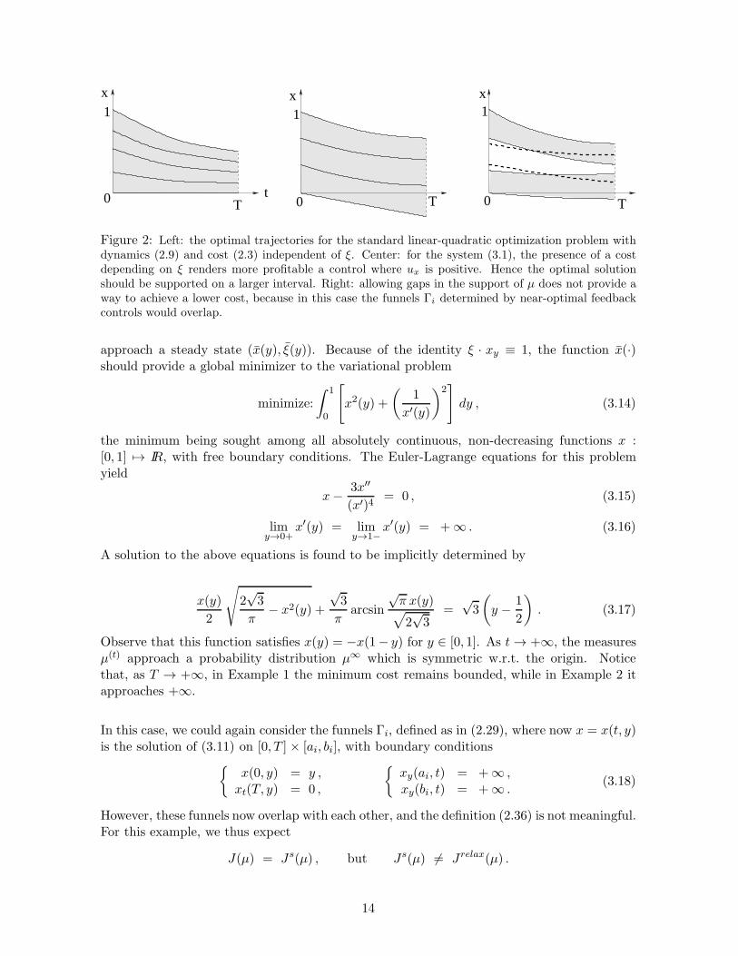
Figure 2: Left: the optimal trajectories for the standard linear-quadratic optimization problem withdynamics (2.9) and cost (2.3) independent of ξ. Center: for the system (3.1), the presence of a costdepending on ξ renders more profitable a control where ux is positive. Hence the optimal solutionshould be supported on a larger interval. Right: allowing gaps in the support of µ does not provide away to achieve a lower cost, because in this case the funnels Γi determined by near-optimal feedbackcontrols would overlap.
approach a steady state (x(y), ξ(y)). Because of the identity ξ · xy ≡ 1, the function x(·)should provide a global minimizer to the variational problem
minimize:
∫ 1
0
[
x2(y) +
(
1
x′(y)
)2]
dy , (3.14)
the minimum being sought among all absolutely continuous, non-decreasing functions x :[0, 1] 7→ IR, with free boundary conditions. The Euler-Lagrange equations for this problemyield
x− 3x′′
(x′)4= 0 , (3.15)
limy→0+
x′(y) = limy→1−
x′(y) = +∞ . (3.16)
A solution to the above equations is found to be implicitly determined by
x(y)
2
√
2√3
π− x2(y) +
√3
πarcsin
√π x(y)√
2√3
=√3
(
y − 1
2
)
. (3.17)
Observe that this function satisfies x(y) = −x(1− y) for y ∈ [0, 1]. As t → +∞, the measuresµ(t) approach a probability distribution µ∞ which is symmetric w.r.t. the origin. Noticethat, as T → +∞, in Example 1 the minimum cost remains bounded, while in Example 2 itapproaches +∞.
In this case, we could again consider the funnels Γi, defined as in (2.29), where now x = x(t, y)is the solution of (3.11) on [0, T ] × [ai, bi], with boundary conditions
{
x(0, y) = y ,xt(T, y) = 0 ,
{
xy(ai, t) = +∞ ,xy(bi, t) = +∞ .
(3.18)
However, these funnels now overlap with each other, and the definition (2.36) is not meaningful.For this example, we thus expect
J(µ) = Js(µ) , but Js(µ) 6= Jrelax(µ) .
14
4 A case where the width of the funnels can be controlled
Example 3. We now consider a case where f depends also on ξ, and one can use thisadditional variable in order to control the width of the funnels Γi, preventing their overlap.Consider again the optimization problem (2.1), but assume that the state of the system evolvesaccording to
{
x = u+ ξ ,
ξ = ux ,(4.1)
with initial datax(0) = y , ξ(0) = h(y) . (4.2)
As before, we assume that y is a random variable uniformly distributed on the interval [0, 1].Otherwise stated, the probability measure µ has density φ = χ[0,1] w.r.t. Lebesgue measure.The corresponding relaxed system is
{
x = u+ ξ ,
ξ = v .(4.3)
By (2.1) and (4.3), to achieve a global minimum one should have
u = ξ =xt2. (4.4)
For each fixed y, writing the Euler-Lagrange equations we find that the optimal solutiont 7→ x(t, y) to the relaxed problem solves the two-point boundary value problem
x− 2x = 0 for t ∈ [0, T ] , x(0, y) = y , x(T, y) = 0 . (4.5)
The optimal solution is thus found to be
x(t, y) =e√2(t−2T ) + e−
√2t
1 + e−2√2T
y . (4.6)
For this relaxed solution, the corresponding variables u, ξ are given by
u(t, y) = ξ(t, y) =xt(t, y)
2=
e√2(t−2T ) − e−
√2t
1 + e−2√2T
y√2. (4.7)
On the other hand, for a fixed y, the map v(·, y) should formally be given by the distributionalderivative of the map t 7→ ξ(t, y). This is a measure containing a point mass of size
ξ(0+, y)− h(y) =e−2
√2T − 1
e−2√2T + 1
y√2− h(y)
at the origin, while its restriction to the open set {t > 0} is absolutely continuous w.r.t. Lebesguemeasure, with density
v(t, y) =1
2xtt(t, y) = x(t, y) =
e√2(t−2T ) + e−
√2t
1 + e−2√2T
y . (4.8)
From the above analysis, we conclude that the infimum among all costs J(µ, u, v), with u, v ∈C2, is provided by
Jrelax(µ) =
∫ 1
0
∫ T
0
(
x2(t, y) +1
2x2t (t, y)
)
dt dy . (4.9)
15
A minimizing sequence of feedback controls (uν , vν)ν≥1 is provided by
uν(t, x) = u(t, x) =e√2(t−2T ) − e−
√2t
e√2(t−2T ) + e−
√2t
x√2,
vν(t, x) =
ν ·(
e−2√2T − 1
e−2√2T + 1
x√2− h(x)
)
if t ∈ [0, ν−1] ,
x if t ∈ [ν−1, T ] .
By performing a suitable cut-off, followed by a mollification, we achieve uν , vν ∈ C2.
This preliminary analysis shows that, for any ε > 0, there exists smooth feedback controlsu∗ = u∗(t, x) and v∗ = v∗(t, x) such that
J (µ, u∗, v∗) ≤ Jrelax(µ) + ε , (4.10)
and, calling x = x∗(t, y), ξ = ξ∗(t, y) the corresponding solutions of (4.2)-(4.3), one has
‖x∗‖C2([0,T ]×[0,1]) ≤ M0 , ‖ξ∗‖C2([0,T ]×[0,1]) ≤ M0 ,
‖u∗‖C2([0,T ]×IR) ≤ M1 , ‖v∗‖C2([0,T ]×IR) ≤ M1 ,(4.11)
x∗y(t, y) ≥ ρ0 > 0 , ‖h(y)‖C2([0,1]) ≤ M2 , (4.12)
for some constants M0,M1,M2, ρ0, possibly depending on ε.
Proposition 2. In the above example one has Js(µ) = Jrelax(µ).
Proof. Given ε > 0, let (u∗, v∗) be a pair of generalized feedback controls for which allthe estimates (4.10)–(4.12) hold. To prove Proposition 2, we need to show that there exists ameasure µ with density φ satisfying ‖φ− φ‖L1 ≤ ε and a feedback control u ∈ C2 such that
J(u, µ) ≤ J (u∗, v∗, µ) + ε . (4.13)
1. Consider the augmented system of ODEs
x = u+ ξ ,
ξ = v ,
η = ηv + z ,
z = wη ,
x(0, y) = y ,
ξ(0, y) = h(y) ,
η(0, y) = 1 ,
z(0, y) = h′(y) .
(4.14)
Here we think of η = xy and z = ξy as an additional variable, while v = ux, w = vx = uxx areadditional controls. Notice that the last two ODEs in (4.14) follow from
(xy)t = uy + ξy = ux xy + ξy , (ξy)t = vy = vx xy .
16
2. For n large, consider the probability distribution µn having density
φn(x).=
n
n− 1if x ∈
[
i− 1
n,
i
n− 1
n2
]
.= [ai, bi], for some i ∈ {1, . . . , n},
0 otherwise.(4.15)
For i = 1, . . . , n, denote by t 7→ xi(t).= x∗(t, ai), t 7→ ξi(t)
.= ξ∗(t, ai) the components of the
solution of (4.2)-(4.3) with y = ai. As a first attempt, one may construct the feedback u bysetting
u(t, x).= u∗(t, xi(t)) + v∗(t, xi(t)) · (x− xi(t)) (4.16)
for x ≈ xi(t). For y ∈ [ai, bi], call t 7→ (x(t, y), ξ(t, y)) the solution of (4.1)-(4.2), with u = ugiven by (4.16). Observe that this construction yields
x(t, ai) = xi(t).= x∗(t, ai) , ξ(t, ai) = ξi(t)
.= ξ∗(t, ai) , t ∈ [0, T ] , 1 ≤ i ≤ n .
Introducing the tubes
Γi.={
(t, x(t, y)) ; t ∈ [0, T ] , y ∈ [ai , bi]}
, (4.17)
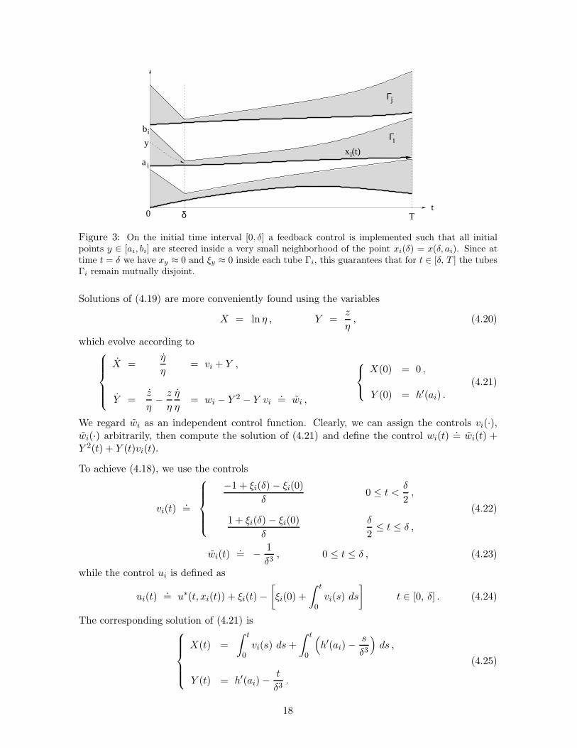
one may hope to define u(t, x) by (4.16) for (t, x) ∈ Γi, and extend u in a smooth way on thecomplementary set ([0, T ]×IR)\∪iΓi . Notice that (4.12) implies x1(t) < x2(t) < · · · < xn(t), sothat the centers of these tubes do not cross each other. Unfortunately, in the present situationthere is no guarantee that the tubes Γi remain disjoint for all t ∈ [0, T ]. We thus need torefine our construction, relying on a global controllability property of the system (4.14). On asmall time interval [0, δ], we will construct a feedback u such that the corresponding solutionof (4.1)-(4.2) satisfies
∣
∣
∣x(δ, y) − xi(δ)∣
∣
∣ < ǫ ,∣
∣
∣ξ(δ, y) − ξi(δ)∣
∣
∣ < ǫ , for all y ∈ [ai, bi] . (4.18)
If (4.18) holds, with ǫ << n−1 suitably small, then for t ∈ [δ, T ], and x ≈ xi(t) the definition(4.16) will provide a feedback with the desired properties. To achieve (4.18) we shall constructa feedback such that xy(δ, y) ≈ 0 and ξy(δ, y) ≈ 0, for all y ∈ [ai, bi].
3. Let δ > 0 be given. Relying on the controllability of the ODE (4.14), for 0 ≤ t ≤ δ andi ∈ {1, . . . , n}, we construct control functions ui(·), vi(·), wi(·) such that the solution of theCauchy problem
x = ui + ξ ,
ξ = vi ,
η = η vi + z ,
z = η wi ,
x(0) = ai ,
ξ(0) = h(ai) ,
η(0) = 1 ,
z(0) = h′(ai) .
(4.19)
satisfies x(t) = xi(t).= x∗(t, ai) for all t ∈ [0, δ] and moreover
ξ(δ) = ξi(δ).= ξ∗(δ, ai), η(δ) ≈ 0, z(δ) ≈ 0.
17
Γ
Γ
ia
ib
ix (t)
0 δ Tt
i
j
y
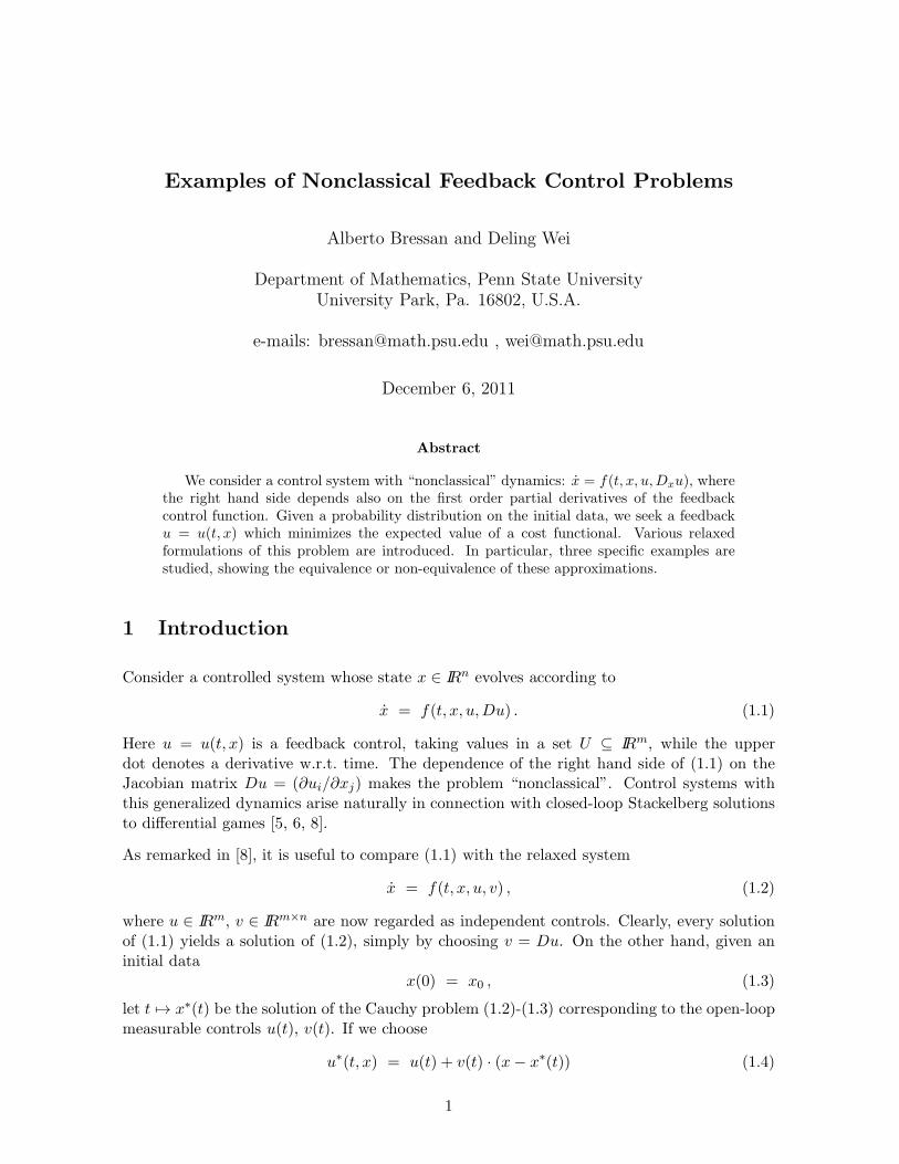
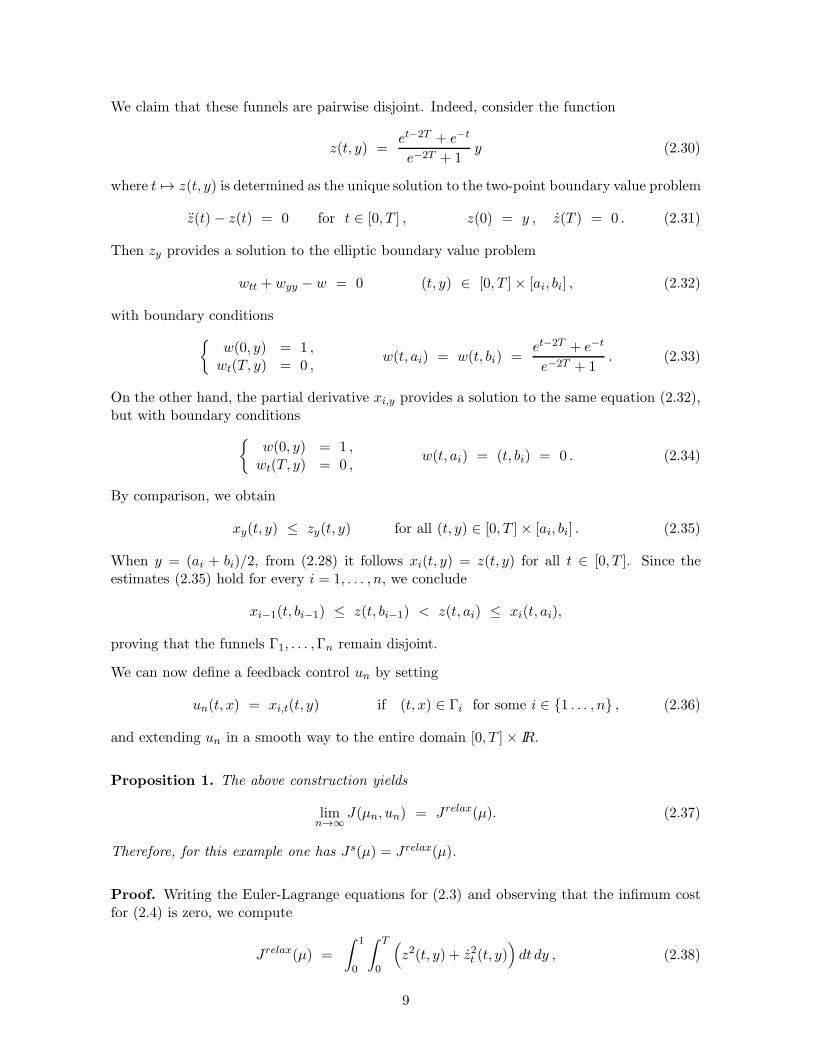
Figure 3: On the initial time interval [0, δ] a feedback control is implemented such that all initialpoints y ∈ [ai, bi] are steered inside a very small neighborhood of the point xi(δ) = x(δ, ai). Since attime t = δ we have xy ≈ 0 and ξy ≈ 0 inside each tube Γi, this guarantees that for t ∈ [δ, T ] the tubesΓi remain mutually disjoint.
Solutions of (4.19) are more conveniently found using the variables
X = ln η , Y =z
η, (4.20)
which evolve according to
X =η
η= vi + Y ,
Y =z
η− z
η
η
η= wi − Y 2 − Y vi
.= wi ,
X(0) = 0 ,
Y (0) = h′(ai) .(4.21)
We regard wi as an independent control function. Clearly, we can assign the controls vi(·),wi(·) arbitrarily, then compute the solution of (4.21) and define the control wi(t)
.= wi(t) +
Y 2(t) + Y (t)vi(t).
To achieve (4.18), we use the controls
vi(t).=
−1 + ξi(δ)− ξi(0)
δ0 ≤ t <
δ
2,
1 + ξi(δ) − ξi(0)
δ
δ
2≤ t ≤ δ ,
(4.22)
wi(t).= − 1
δ3, 0 ≤ t ≤ δ , (4.23)
while the control ui is defined as
ui(t).= u∗(t, xi(t)) + ξi(t)−
[
ξi(0) +
∫ t
0vi(s) ds
]
t ∈ [0, δ] . (4.24)
The corresponding solution of (4.21) is
X(t) =
∫ t
0vi(s) ds+
∫ t
0
(
h′(ai)−s
δ3
)
ds ,
Y (t) = h′(ai)−t
δ3.
(4.25)
18

In particular, at t = δ one has
X(δ) = ξi(δ) − ξi(0) + h′(ai)δ −1
2δ, Y (δ) = h′(ai)−
1
δ2. (4.26)
Going back to original variables η, z, one obtains
η(δ) = exp(
X(δ))
= exp(
ξi(δ) − ξi(0) + h′(ai)δ −1
2δ
)
,
z(δ) = Y (δ)η(δ) =(
h′(ai)−1
δ2
)
exp(
ξi(δ)− ξi(0) + h′(ai)δ −1
2δ
)
.
(4.27)
Moreover, by the definition of w in (4.21), the control wi = wi + Y 2 + Y vi is given by
wi(t) =
− 1
δ3+(
h′(ai)−t
δ3
)2+(−1 + ξi(δ) − ξi(0)
δ
)(
h′(ai)−t
δ3
)
, 0 ≤ t <δ
2,
− 1
δ3+(
h′(ai)−t
δ3
)2+(1 + ξi(δ) − ξi(0)
δ
)(
h′(ai)−t
δ3
)
,δ
2≤ t ≤ δ .
(4.28)By (4.22), (4.23), and (4.25), for δ > 0 sufficiently small we have the estimates
|vi(t)| ≤ 2
δ, |Y (t)| ≤ 2
δ2, |wi(t)| ≤ 5
δ4, for all t ∈ [0, δ] . (4.29)
Moreover, by(4.24), the solution (x(·), ξ(·)) of (4.19) satisfies
x(t) = ui(t) + ξ(t) = u∗(t, xi(t)) + ξi(t) = xi(t) , for all t ∈ [0, δ] .
4. On a suitable neighborhood of each trajectory t 7→ xi(t), we then define the feedbackcontrol u as
u(t, x).=
ui(t) + (x− xi(t)) · vi(t) +(x− xi(t))
2
2· wi(t) , t ∈ [0, δ] ,
u∗(t, xi(t)) + (x− xi(t)) · v∗(t, xi(t)) , t ∈ [δ, T ] .
(4.30)
The corresponding solution of (4.1) with initial data (4.2) will be denoted by t 7→ (x(t, y), ξ(t, y)).We can then extend u in a smooth way (w.r.t. the x-variable) on the complement of the set∪1≤i≤nΓi. Notice that, by choosing n = n(δ) >> δ−1, we can achieve the convergence
‖u− u∗‖L∞([δ,T ]×IR) → 0 as δ → 0. (4.31)
For every i ∈ {1, . . . , n}, the above construction yields
x(t, ai) = xi(t) t ∈ [0, T ] .
∣
∣ξ(t, ai)∣
∣ =
∣
∣
∣
∣
ξi(0) +
∫ t
0vi(s) ds
∣
∣
∣
∣
≤ M0(1 + δ) + 1 t ∈ [0, δ] , (4.32)
ξ(δ , ai) = ξi(δ) .
19
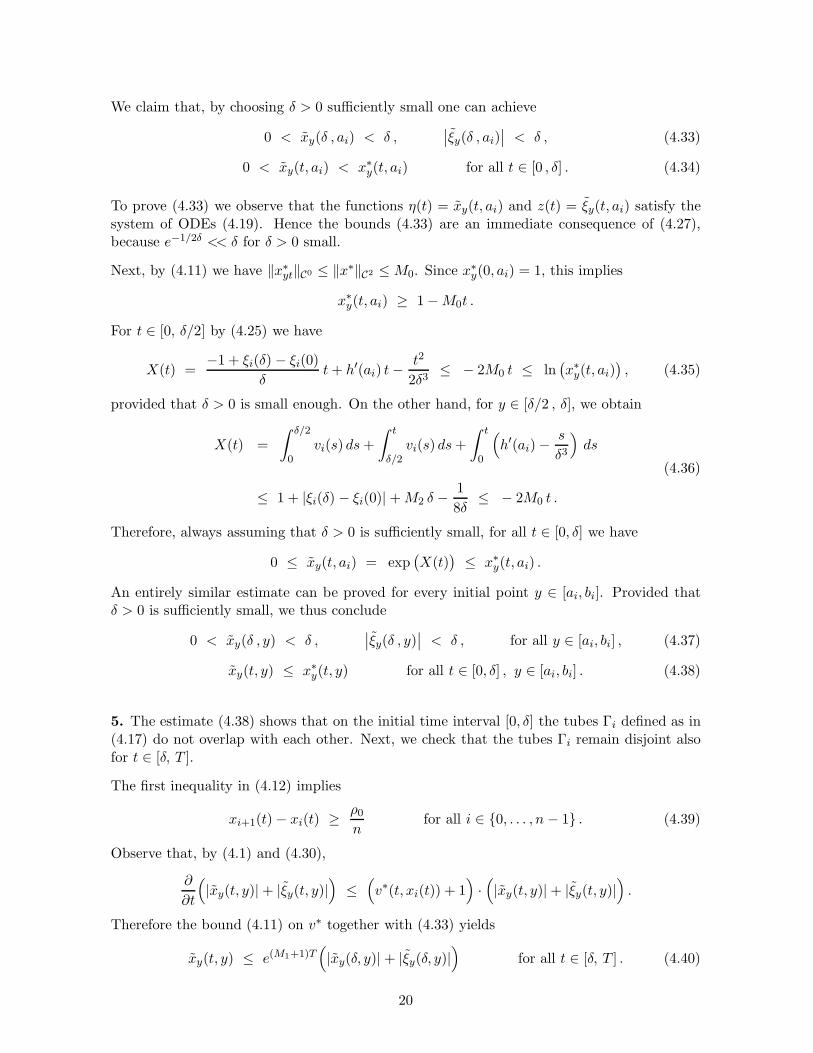
We claim that, by choosing δ > 0 sufficiently small one can achieve
0 < xy(δ , ai) < δ ,∣
∣ξy(δ , ai)∣
∣ < δ , (4.33)
0 < xy(t, ai) < x∗y(t, ai) for all t ∈ [0 , δ] . (4.34)
To prove (4.33) we observe that the functions η(t) = xy(t, ai) and z(t) = ξy(t, ai) satisfy thesystem of ODEs (4.19). Hence the bounds (4.33) are an immediate consequence of (4.27),because e−1/2δ << δ for δ > 0 small.
Next, by (4.11) we have ‖x∗yt‖C0 ≤ ‖x∗‖C2 ≤ M0. Since x∗y(0, ai) = 1, this implies
x∗y(t, ai) ≥ 1−M0t .
For t ∈ [0, δ/2] by (4.25) we have
X(t) =−1 + ξi(δ) − ξi(0)
δt+ h′(ai) t−
t2
2δ3≤ − 2M0 t ≤ ln
(
x∗y(t, ai))
, (4.35)
provided that δ > 0 is small enough. On the other hand, for y ∈ [δ/2 , δ], we obtain
X(t) =
∫ δ/2
0vi(s) ds+
∫ t
δ/2vi(s) ds+
∫ t
0
(
h′(ai)−s
δ3
)
ds
≤ 1 + |ξi(δ) − ξi(0)| +M2 δ −1
8δ≤ − 2M0 t .
(4.36)
Therefore, always assuming that δ > 0 is sufficiently small, for all t ∈ [0, δ] we have
0 ≤ xy(t, ai) = exp(
X(t))
≤ x∗y(t, ai) .
An entirely similar estimate can be proved for every initial point y ∈ [ai, bi]. Provided thatδ > 0 is sufficiently small, we thus conclude
0 < xy(δ , y) < δ ,∣
∣ξy(δ , y)∣
∣ < δ , for all y ∈ [ai, bi] , (4.37)
xy(t, y) ≤ x∗y(t, y) for all t ∈ [0, δ] , y ∈ [ai, bi] . (4.38)
5. The estimate (4.38) shows that on the initial time interval [0, δ] the tubes Γi defined as in(4.17) do not overlap with each other. Next, we check that the tubes Γi remain disjoint alsofor t ∈ [δ, T ].
The first inequality in (4.12) implies
xi+1(t)− xi(t) ≥ ρ0n
for all i ∈ {0, . . . , n − 1} . (4.39)
Observe that, by (4.1) and (4.30),
∂
∂t
(
|xy(t, y)|+ |ξy(t, y)|)
≤(
v∗(t, xi(t)) + 1)
·(
|xy(t, y)|+ |ξy(t, y)|)
.
Therefore the bound (4.11) on v∗ together with (4.33) yields
xy(t, y) ≤ e(M1+1)T(
|xy(δ, y)| + |ξy(δ, y)|)
for all t ∈ [δ, T ] . (4.40)
20
For y ∈ [ai, bi] and t ∈ [δ, T ] we have
x(t, y)− xi(t) ≤∫ y
ai
xy(t, z) dz ≤ (bi − ai) · supy∈[0,1]
xy(t, y) ≤ ρ0n
, (4.41)
provided that
e(M1+1)T · supy
(
|xy(δ, y)| + |ξ(δ, y)|)
≤ ρ0 .
Recalling (4.33) we can now choose δ > 0 small enough so that e(M1+1)T 4δ < ρ0. Then wechoose n = n(δ) >> 1/δ large enough so that, by continuity, the estimates
(
|xy(δ, y)| + |ξ(δ, y)|)
< 4δ <ρ0
e(M1+1)T
remain valid for every y ∈ [ai, bi], i = 1, . . . , n. By (4.39) and (4.41), this implies that thetubes Γi remain mutually disjoint also for t ∈ [δ, T ].
6. It is clear that the sequence of densities φn in (4.15) converges to φ = χ[0,1]
as n → ∞.
Having chosen δ > 0 and n = n(δ) >> δ−1 as before, let u = u(t, x) be a feedback controlsatisfying (4.30) on each tube Γi, extended in a smooth way outside the union ∪n
i=1Γi. Itremains to show that, as δ → 0, the expected cost for the feedback u approaches J (u∗, v∗, µ).Indeed, on the initial interval [0, δ], by (4.32) all functions x, ξ, u remain uniformly boundedas δ → 0. Therefore
n
n− 1·
n∑
i=1
∫ δ
0
∫ bi
ai
(
x2(t, y) + ξ2(t, y) + u2(t, x(t, y)))
dy dt ≤ Cδ . (4.42)
To see what happens on the remaining interval [δ, T ], consider the quantities
An.=
n
n− 1·
n∑
i=1
∫ T
δ
∫ bi
ai
(
x2(t, y) + ξ2(t, y) + u2(t, x(t, y)))
dy dt
Bn.=
1
n·
n∑
i=1
∫ T
δ
(
(x∗)2(t, ai) + (ξ∗)2(t, ai) + (u∗)2(t, xi(t)))
dy dt .
Recalling (4.31) we have |An −Bn| → 0 as δ → 0 and n = n(δ) → ∞. Moreover,
limn→∞
Bn =
∫ T
0
∫ 1
0
(
(x∗)2(t, y) + (ξ∗)2(t, y) + (u∗)2(t, x∗(t, y)))
dy dt = J (u∗, v∗, µ) .
This completes the proof.
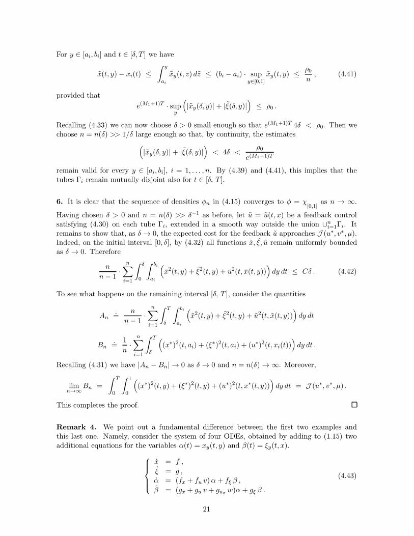
Remark 4. We point out a fundamental difference between the first two examples andthis last one. Namely, consider the system of four ODEs, obtained by adding to (1.15) twoadditional equations for the variables α(t) = xy(t, y) and β(t) = ξy(t, x).
x = f ,
ξ = g ,α = (fx + fu v)α+ fξ β ,
β = (gx + gu v + guxw)α + gξ β .
(4.43)
21
Here v = ux and w = uxx are regarded as independent control functions. In the first twoexamples this system is not controllable. Indeed, no matter what controls are implemented,in Example 1 we always have ξ(t)− α(t) ≡ 0, while in Example 2 one has ξ(t) · α(t) ≡ 1. Onthe other hand, in Example 3 there is no functional relation between ξ and α. We expect thatthis controllability property of the extended system (4.43) should play a key role, determiningthe equality between the minimal costs Js(µ) and Jrelax(µ).
References
[1] T. Basar and G. J. Olsder, Dynamic Noncooperative Game Theory. Reprint of the secondedition. SIAM, Philadelphia, 1999.
[2] A. Bressan and D. Wei, Non-classical problems of optimal feedback control. Preprint,2011.
[3] L. Cesari, Optimization - Theory and Applications, Springer-Verlag, 1983.
[4] E. J. Dockner, S. Jorgensen, N. V. Long, and G. Sorger, Differential Games in Economicsand Management Science. Cambridge University Press, 2000.
[5] M. Jungers, E. Trelat, and H. Abou-Kandil, Min-max and max-min Stackelberg strategieswith closed-loop information structure. ESAIM, Control Optim. Calc. Var., to appear.
[6] J. Medanic, Closed-loop Stackelberg strategies in linear-quadratic problems, IEEE Trans.Autom. Control, 23 (1978), 632-637.
[7] B. M. Miller, B.M. and Y. E. Rubinovich, Impulsive Control in Continuous and Discrete-Continuous Systems, Kluwer, New York, 2003.
[8] G. P. Papavassilopoulos and J. B. Cruz, Nonclassical control problems and Stackelberggames, IEEE Transactions on Automatic Control, 24 (1979), 155-166.
[9] M. H. Protter and H. F. Weinberger, Maximum Principles in Differential Equations,Prentice Hall, 1967.
[10] R. W. Rishel, An extended Pontryagin principle for control systems whose control lawscontain measures, SIAM J. Control 3 (1965), 191-205.
[11] G. N. Silva and R. B. Vinter, Measure driven differential inclusions, J. Math. Anal. Appl.202 (1996), 727-746.
22