Example of Global Data-Flow Analysis

Reaching Definitions

We will illustrate global data-flow analysis with the computation of reaching definitions for a very simple and structured programming language.

We want to compute for each block b of the program the set REACHES(b) of the statements that compute values which are available on entry to b.

An assignment statement of the form x:=E or a read statement of the form read x must define x.

A call statement call sub(x) where x is passed by reference or an assignment of the form *q:= y where nothing is known about pointer q, may define x.

We say that a statement s that must or may define a variable x reaches a block b if there is a path from s to b such that there is no statement y in the path that kills s. That is, there is no statement y that must define x. A block may be reached by a must define statement s as well as a may define statement on the same variable that appears after s in a path to b.

We must be conservative to guarantee correct transformations. In the case of reaching definitions conservative is to assume that a definition can reach a point even if it might not.

1

Data-Flow Equations

Consider the following language:

S ::= id:=expression | S;S | if expression then S else S | do S while expression

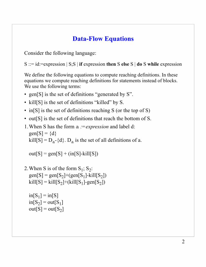
We define the following equations to compute reaching definitions. In these equations we compute reaching definitions for statements instead of blocks. We use the following terms:• gen[S] is the set of definitions “generated by S”.• kill[S] is the set of definitions “killed” by S. • in[S] is the set of definitions reaching S (or the top of S)• out[S] is the set of definitions that reach the bottom of S.1.When S has the form a :=expression and label d:

gen[S] = {d}kill[S] = Da-{d}. Da is the set of all definitions of a.

out[S] = gen[S] + (in[S]-kill[S])

2.When S is of the form S1; S2:gen[S] = gen[S2]+(gen[S1]-kill[S2])kill[S] = kill[S2]+(kill[S1]-gen[S2])

in[S1] = in[S]in[S2] = out[S1]out[S] = out[S2]

2

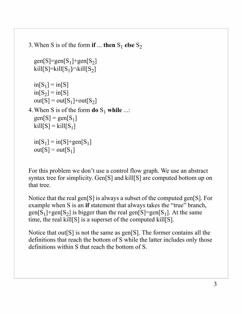
3.When S is of the form if ... then S1 else S2

gen[S]=gen[S1]+gen[S2]kill[S]=kill[S1]∩kill[S2]

in[S1] = in[S]in[S2] = in[S]out[S] = out[S1]+out[S2]

4.When S is of the form do S1 while ...:gen[S] = gen[S1]kill[S] = kill[S1]

in[S1] = in[S]+gen[S1]out[S] = out[S1]

For this problem we don’t use a control flow graph. We use an abstract syntax tree for simplicity. Gen[S] and kill[S] are computed bottom up on that tree.

Notice that the real gen[S] is always a subset of the computed gen[S]. For example when S is an if statement that always takes the “true” branch, gen[S1]+gen[S2] is bigger than the real gen[S]=gen[S1]. At the same time, the real kill[S] is a superset of the computed kill[S].

Notice that out[S] is not the same as gen[S]. The former contains all the definitions that reach the bottom of S while the latter includes only those definitions within S that reach the bottom of S.

3

In[S] and out[S] are computed starting at the statement S0 representing the whole program.

Algorithm IN-OUT: Compute in[S] and out[S] for all statements S

Input: An abstract syntax tree of program S0 and the gen and kill sets for all the statements within the program.

Output:in[S] and out[S] for all statements within the program

4

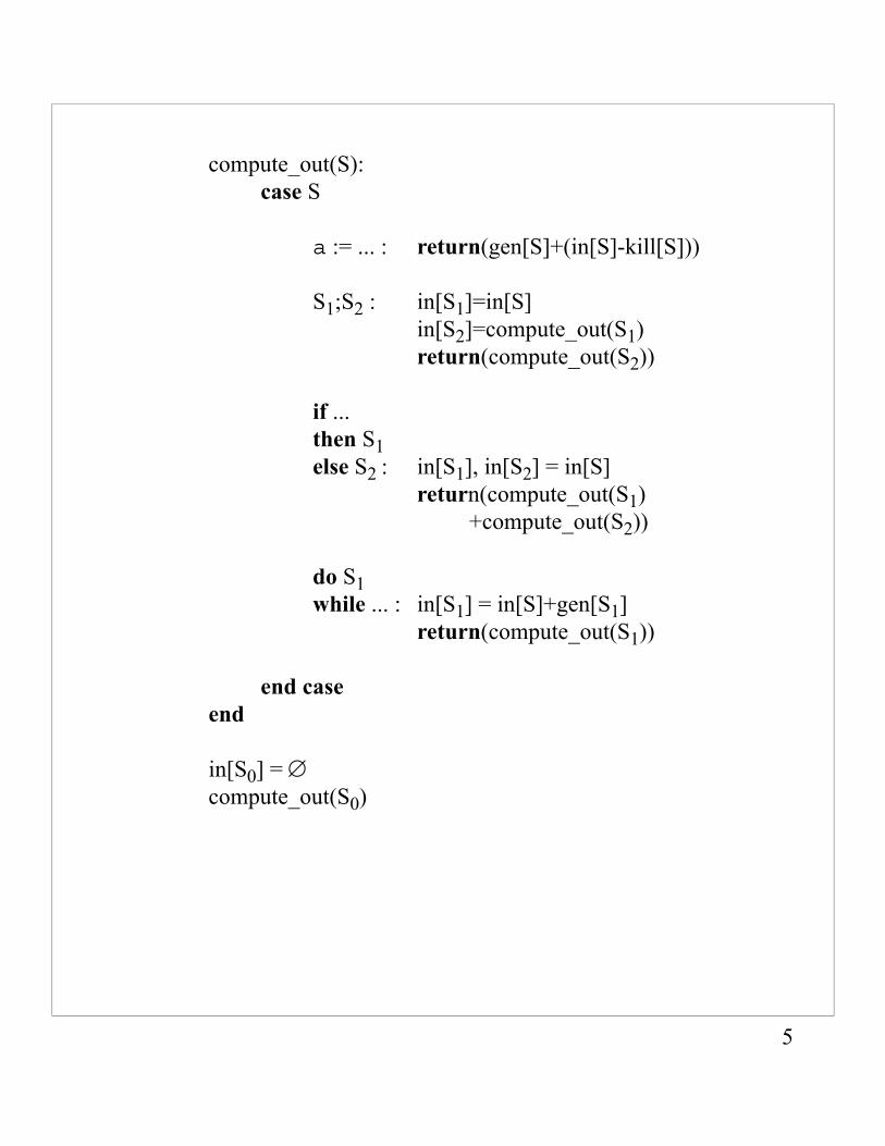
compute_out(S):case S

a := ... : return(gen[S]+(in[S]-kill[S]))

S1;S2 : in[S1]=in[S]in[S2]=compute_out(S1)return(compute_out(S2))

if ... then S1else S2 : in[S1], in[S2] = in[S]

return(compute_out(S1)+compute_out(S2))

do S1while ... : in[S1] = in[S]+gen[S1]

return(compute_out(S1))

end caseend

in[S0] = ∅compute_out(S0)

5

The sets of statements can be represented with bit vectors. Then unions and intersections take the form of or and operations. Only the statements that assign values to program variables have to be taken into account. That is statements (or instructions) assigning to compiler-generated temporaries can be ignored.

In an implementation it is better to do the computations for the basic blocks only. The reaching sets for each statement can be then obtained by applying rule 2 above.

6

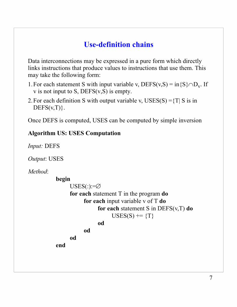
Use-definition chains

Data interconnections may be expressed in a pure form which directly links instructions that produce values to instructions that use them. This may take the following form:1.For each statement S with input variable v, DEFS(v,S) = in{S}∩Dv. If

v is not input to S, DEFS(v,S) is empty.2.For each definition S with output variable v, USES(S) ={T| S is in

DEFS(v,T)}.

Once DEFS is computed, USES can be computed by simple inversion

Algorithm US: USES Computation

Input: DEFS

Output: USES

Method:begin

USES(:):=∅for each statement T in the program do

for each input variable v of T dofor each statement S in DEFS(v,T) do

USES(S) += {T}od

odod

end

7

8

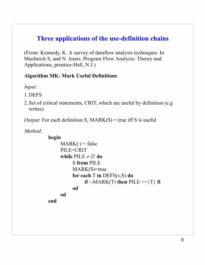
Three applications of the use-definition chains

(From: Kennedy, K. A survey of dataflow analysis techniques. In Muchnick S, and N. Jones. Program Flow Analysis: Theory and Applications, prentice-Hall, N.J.)

Algorithm MK: Mark Useful Definitions

Input:1.DEFS2.Set of critical statements, CRIT, which are useful by definition (e.g

writes)

Output: For each definition S, MARK(S) = true iff S is useful

Method:begin

MARK(:) = falsePILE=CRITwhile PILE ≠ ∅ do

S from PILEMARK(S)=truefor each T in DEFS(v,S) do

if ¬MARK(T) then PILE +={T} fiod

odend

9

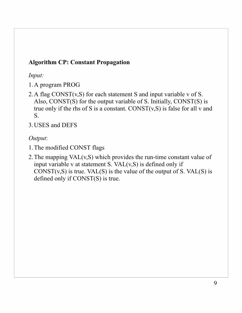
Algorithm CP: Constant Propagation

Input:1.A program PROG2.A flag CONST(v,S) for each statement S and input variable v of S.

Also, CONST(S) for the output variable of S. Initially, CONST(S) is true only if the rhs of S is a constant. CONST(v,S) is false for all v and S.

3.USES and DEFS

Output: 1.The modified CONST flags2.The mapping VAL(v,S) which provides the run-time constant value of

input variable v at statement S. VAL(v,S) is defined only if CONST(v,S) is true. VAL(S) is the value of the output of S. VAL(S) is defined only if CONST(S) is true.

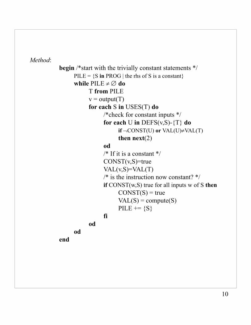
Method:begin /*start with the trivially constant statements */

PILE = {S in PROG | the rhs of S is a constant}while PILE ≠ ∅ do

T from PILEv = output(T)for each S in USES(T) do

/*check for constant inputs */for each U in DEFS(v,S)-{T} do

if ¬CONST(U) or VAL(U)≠VAL(T)then next(2)

od/* If it is a constant */CONST(v,S)=trueVAL(v,S)=VAL(T)/* is the instruction now constant? */if CONST(w,S) true for all inputs w of S then

CONST(S) = trueVAL(S) = compute(S)PILE += {S}

fiod

odend

10

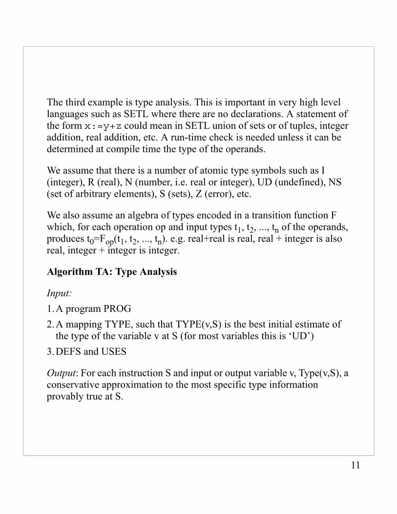
The third example is type analysis. This is important in very high level languages such as SETL where there are no declarations. A statement of the form x:=y+z could mean in SETL union of sets or of tuples, integer addition, real addition, etc. A run-time check is needed unless it can be determined at compile time the type of the operands.

We assume that there is a number of atomic type symbols such as I (integer), R (real), N (number, i.e. real or integer), UD (undefined), NS (set of arbitrary elements), S (sets), Z (error), etc.

We also assume an algebra of types encoded in a transition function F which, for each operation op and input types t1, t2, ..., tn of the operands, produces t0=Fop(t1, t2, ..., tn). e.g. real+real is real, real + integer is also real, integer + integer is integer.

Algorithm TA: Type Analysis

Input:1.A program PROG2.A mapping TYPE, such that TYPE(v,S) is the best initial estimate of

the type of the variable v at S (for most variables this is ‘UD’)3.DEFS and USES

Output: For each instruction S and input or output variable v, Type(v,S), a conservative approximation to the most specific type information provably true at S.

11

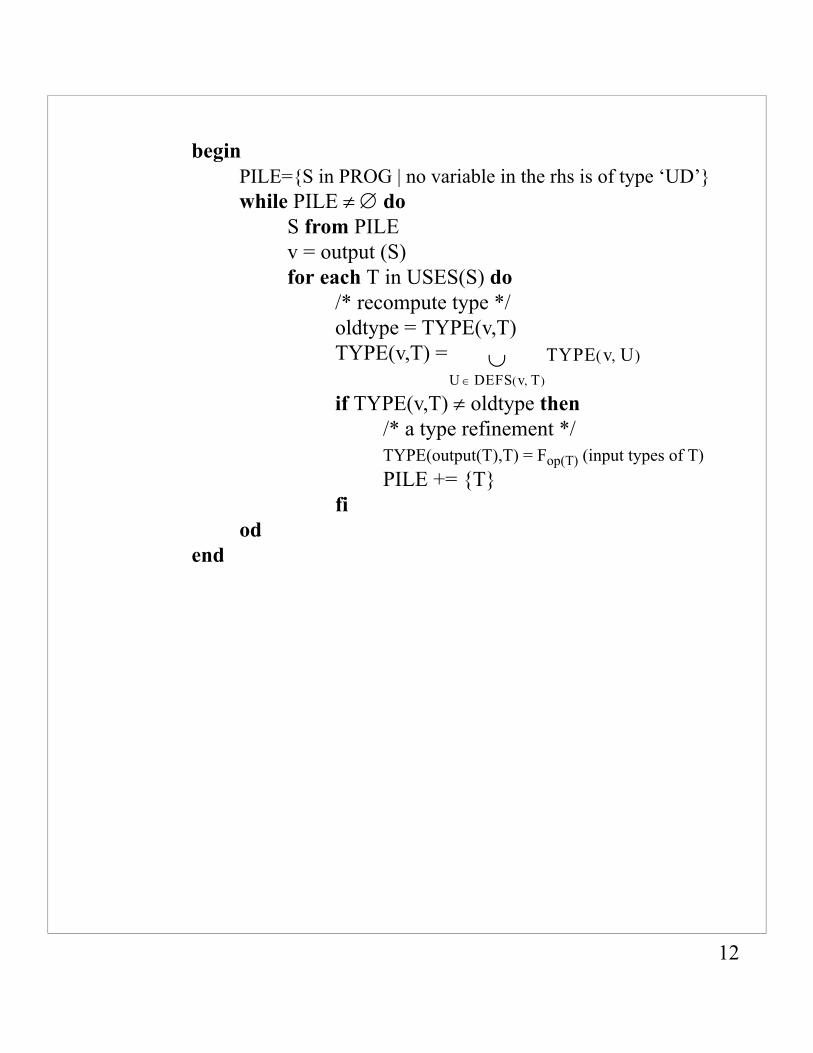
beginPILE={S in PROG | no variable in the rhs is of type ‘UD’}while PILE ≠ ∅ do

S from PILEv = output (S)for each T in USES(S) do

/* recompute type */oldtype = TYPE(v,T)TYPE(v,T) =

if TYPE(v,T) ≠ oldtype then/* a type refinement */TYPE(output(T),T) = Fop(T) (input types of T)PILE += {T}

fiod

end

TYPE v U,( )U DEFS v T,( )∈

∪

12

Some simple iterative algorithms for data flow analysis

The data flow analysis above was done assuming a structured program and operated on an abstract syntax tree.

One simple approach that works even when the flow graph is not reducible is to use iterative algorithms.

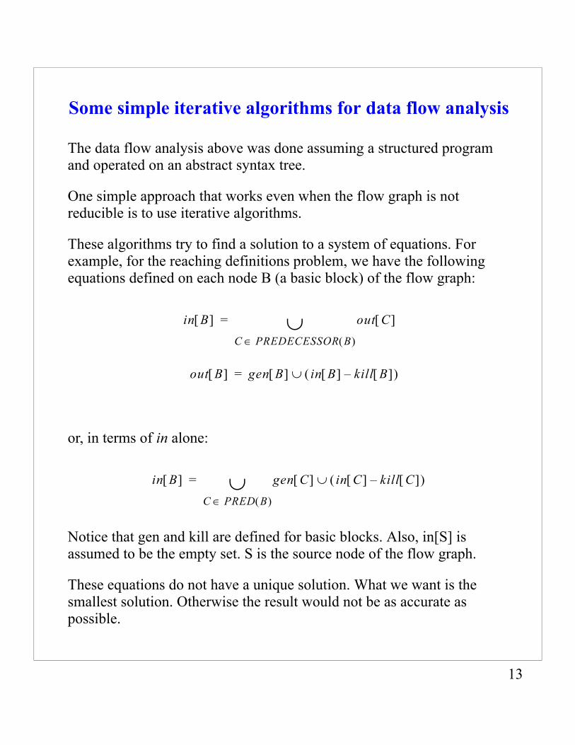
These algorithms try to find a solution to a system of equations. For example, for the reaching definitions problem, we have the following equations defined on each node B (a basic block) of the flow graph:

in B[ ] out C[ ]

C PREDECESSOR B( )∈∪=

or, in terms of in alone:

in B[ ] gen C[ ] in C[ ] kill C[ ]–( )∪

C PRED B( )∈∪=

Notice that gen and kill are defined for basic blocks. Also, in[S] is assumed to be the empty set. S is the source node of the flow graph.

These equations do not have a unique solution. What we want is the smallest solution. Otherwise the result would not be as accurate as possible.

out B[ ] gen B[ ] in B[ ] kill B[ ]–( )∪=

13

There are other important problems that can also be expressed as systems of equations.

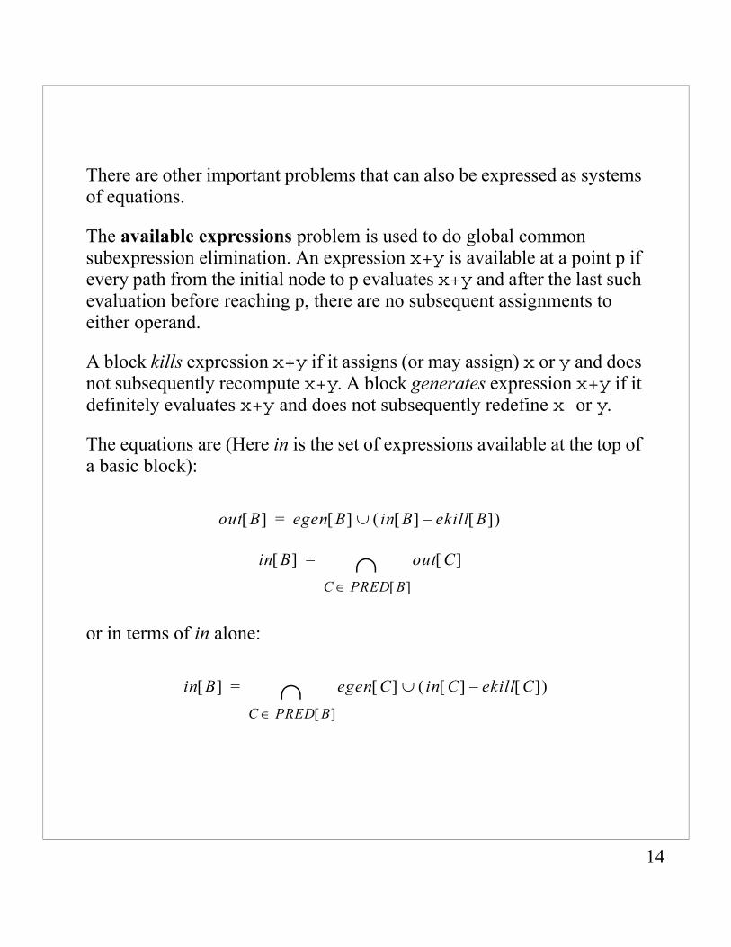
The available expressions problem is used to do global common subexpression elimination. An expression x+y is available at a point p if every path from the initial node to p evaluates x+y and after the last such evaluation before reaching p, there are no subsequent assignments to either operand.

A block kills expression x+y if it assigns (or may assign) x or y and does not subsequently recompute x+y. A block generates expression x+y if it definitely evaluates x+y and does not subsequently redefine x or y.

The equations are (Here in is the set of expressions available at the top of a basic block):

out B[ ] egen B[ ] in B[ ] ekill B[ ]–( )∪=

in B[ ] out C[ ]

C PRED B[ ]∈∩=

or in terms of in alone:

in B[ ] egen C[ ] in C[ ] ekill C[ ]–( )∪

C PRED B[ ]∈∩=

14

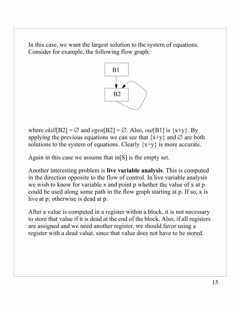
In this case, we want the largest solution to the system of equations. Consider for example, the following flow graph:

B1

B2

where ekill[B2] = ∅ and egen[B2] = ∅. Also, out[B1] is {x+y}. By applying the previous equations we can see that {x+y} and ∅ are both solutions to the system of equations. Clearly {x+y} is more accurate.

Again in this case we assume that in[S] is the empty set.

Another interesting problem is live variable analysis. This is computed in the direction opposite to the flow of control. In live variable analysis we wish to know for variable x and point p whether the value of x at p could be used along some path in the flow graph starting at p. If so, x is live at p; otherwise is dead at p.

After a value is computed in a register within a block, it is not necessary to store that value if it is dead at the end of the block. Also, if all registers are assigned and we need another register, we should favor using a register with a dead value, since that value does not have to be stored.

15

Let def[B] be the set of variables definitively assigned values in B prior to any use of the variable in B, and let use[B] be the set of variables whose values may be used in B prior to any definition of the variable.

The equations are (Here out[B] are the variables live at the end of the block, and in[B], the variables live just before block B.

in B[ ] use B[ ] out B[ ] def B[ ]–( )∪=

out B[ ] in C[ ]

C SUCESSOR B( )∈∪=

or in terms of out alone:

out B[ ] use C[ ] out C[ ] def C[ ]–( )∪

C SUC B( )∈∪=

Finally, we have the problem of identifying very busy expressions. An expression that is evaluated regardless of the path taken from a given point is said to be very busy at that point.

We define egen[B] to be the set of expressions that are evaluated in basic block B before any of the operands are assigned to (if at all) in the block.

16

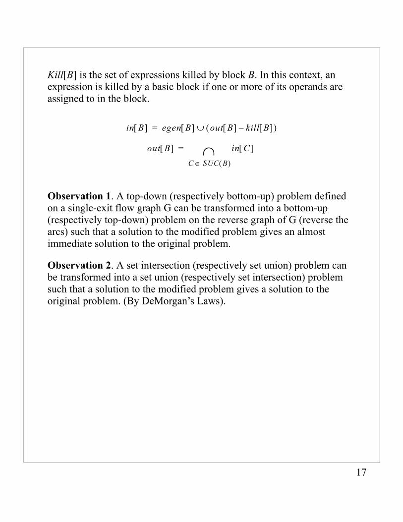
Kill[B] is the set of expressions killed by block B. In this context, an expression is killed by a basic block if one or more of its operands are assigned to in the block.

in B[ ] egen B[ ] out B[ ] kill B[ ]–( )∪=

out B[ ] in C[ ]

C SUC B( )∈∩=

Observation 1. A top-down (respectively bottom-up) problem defined on a single-exit flow graph G can be transformed into a bottom-up (respectively top-down) problem on the reverse graph of G (reverse the arcs) such that a solution to the modified problem gives an almost immediate solution to the original problem.

Observation 2. A set intersection (respectively set union) problem can be transformed into a set union (respectively set intersection) problem such that a solution to the modified problem gives a solution to the original problem. (By DeMorgan’s Laws).

17

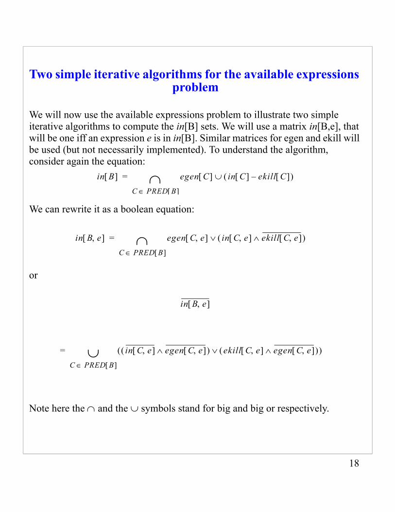
Two simple iterative algorithms for the available expressions problem

We will now use the available expressions problem to illustrate two simple iterative algorithms to compute the in[B] sets. We will use a matrix in[B,e], that will be one iff an expression e is in in[B]. Similar matrices for egen and ekill will be used (but not necessarily implemented). To understand the algorithm, consider again the equation:

in B[ ] egen C[ ] in C[ ] ekill C[ ]–( )∪

C PRED B[ ]∈∩=

We can rewrite it as a boolean equation:

in B e,[ ] egen C e,[ ] in C e,[ ] ekill C e,[ ]∧( )∨

C PRED B[ ]∈∩=

or

in B e,[ ]

in C e,[ ] egen C e,[ ]∧( ) ekill C e,[ ] egen C e,[ ]∧( )∨( )

C PRED B[ ]∈∪=

Note here the ∩ and the ∪ symbols stand for big and big or respectively.

18

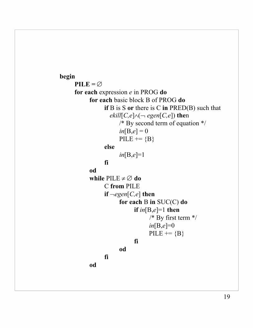
beginPILE = ∅for each expression e in PROG do

for each basic block B of PROG doif B is S or there is C in PRED(B) such that

ekill[C,e]∧(¬ egen[C,e]) then/* By second term of equation */in[B,e] = 0PILE += {B}

elsein[B,e]=1

fiodwhile PILE ≠ ∅ do

C from PILEif ¬egen[C,e] then

for each B in SUC(C) doif in[B,e]=1 then

/* By first term */in[B,e]=0PILE += {B}

fiod

fiod

19

20

Theorem. The previous algorithm terminates and is correct.

Proof

Termination. For each expression e, no node is placed in PILE more than once and each iteration of the while loop removes an entry from PILE.

Correctness. in[B,e] should be 0 iff either:1.There is a path from S to B such that e is not generated in any node

preceding B on this path or2. there is a path to B such that e is killed in the first node of this path and

not subsequently generated.

If in[B,e] is set to zero because of the second term of the equation clearly either 1 or 2 holds. A straightforward induction on the number of iterations of the while loop shows that if in[B,e] is set to zero because of the first term of the equation, then 1 or 2 must hold.

Conversely if 1 or 2 holds, then a straightforward induction shows that in[B,e] is eventually set to 0.

Theorem The algorithm requires at most O(mr) elementary steps, where m is the number of expressions and r is the number of arcs.

Proof The “for each basic block” loop takes O(r) steps. While loop considers each arc once. Therefore O(r). Outermost loop is m iterations and r≥n-1. Therefore O(mr)

21

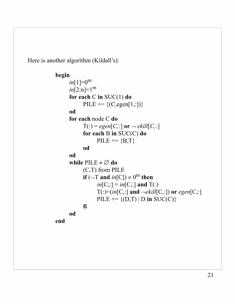
Here is another algorithm (Kildall’s):

beginin[1]=0m

in[2:n]=1m

for each C in SUC(1) doPILE += {(C,egen[1,:])}

odfor each node C do

T(:) = egen[C,:] or ¬ ekill[C,:]for each B in SUC(C) do

PILE += {B,T}od

odwhile PILE ≠ ∅ do

(C,T) from PILEif (¬T and in[C]) ≠ 0m then

in[C,:] = in[C,:] and T(:)T(:)=(in[C,:] and ¬ekill[C,:]) or egen[C,:]PILE += {(D,T) | D in SUC(C)}

fiod

end

22

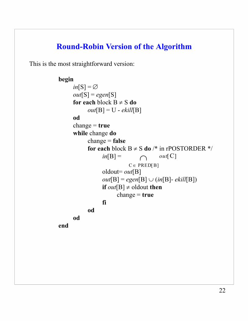
Round-Robin Version of the Algorithm

This is the most straightforward version:

beginin[S] = ∅out[S] = egen[S]for each block B ≠ S do

out[B] = U - ekill[B]odchange = truewhile change do

change = falsefor each block B ≠ S do /* in rPOSTORDER */

in[B] =

oldout= out[B]out[B] = egen[B] ∪ (in[B]- ekill[B])if out[B] ≠ oldout then

change = truefi

odod

end

out C[ ]

C PRED B[ ]∈∩

23

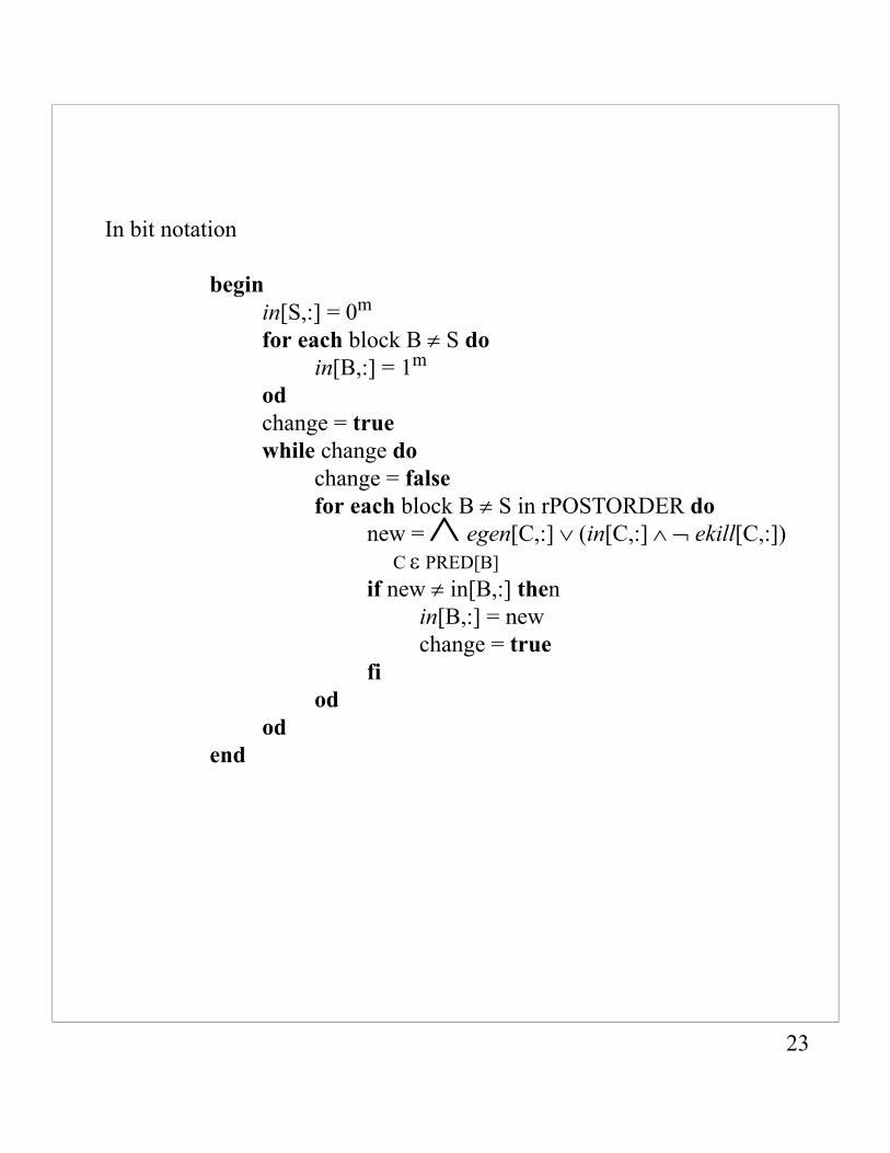
In bit notation

beginin[S,:] = 0m

for each block B ≠ S doin[B,:] = 1m

odchange = truewhile change do

change = falsefor each block B ≠ S in rPOSTORDER do

new = ∧ egen[C,:] ∨ (in[C,:] ∧ ¬ ekill[C,:])

if new ≠ in[B,:] thenin[B,:] = newchange = true

fiod

odend

C ε PRED[B]

24

To study the complexity of the above algorithm we need the following definition.

Definition Loop-connectedness of a reducible flow graph is the largest number of back arcs on any cycle- free path of the graph.

Lemma Any cycle-free path in a reducible flow graph beginning with the initial node is monotonically increasing in rPOSTORDER.

Lemma The while loop in the above algorithm is executed at most d+2 times for a reducible flow graph, where d is the loop connectedness of the graph.

Proof A 0 propagates from its point of origin (either from the source of from a “kill”) to the place where it is needed in d+1 iterations if it must propagate along a path P of d back arcs. One more iteration is needed to reach the tail of the first back arc.

Theorem If we ignore initialization, the previous algorithm takes at most (d+2)(r+n) bit vector steps; that is O(dr) or O(r2) bit vector steps.

25

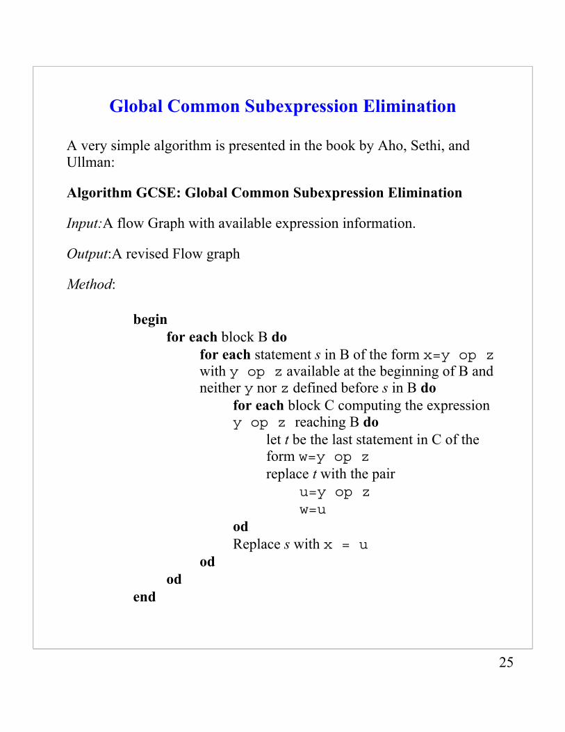
Global Common Subexpression Elimination

A very simple algorithm is presented in the book by Aho, Sethi, and Ullman:

Algorithm GCSE: Global Common Subexpression Elimination

Input:A flow Graph with available expression information.

Output:A revised Flow graph

Method:

beginfor each block B do

for each statement s in B of the form x=y op z with y op z available at the beginning of B and neither y nor z defined before s in B do

for each block C computing the expression y op z reaching B do

let t be the last statement in C of the form w=y op zreplace t with the pair

u=y op zw=u

odReplace s with x = u

odod

end

26

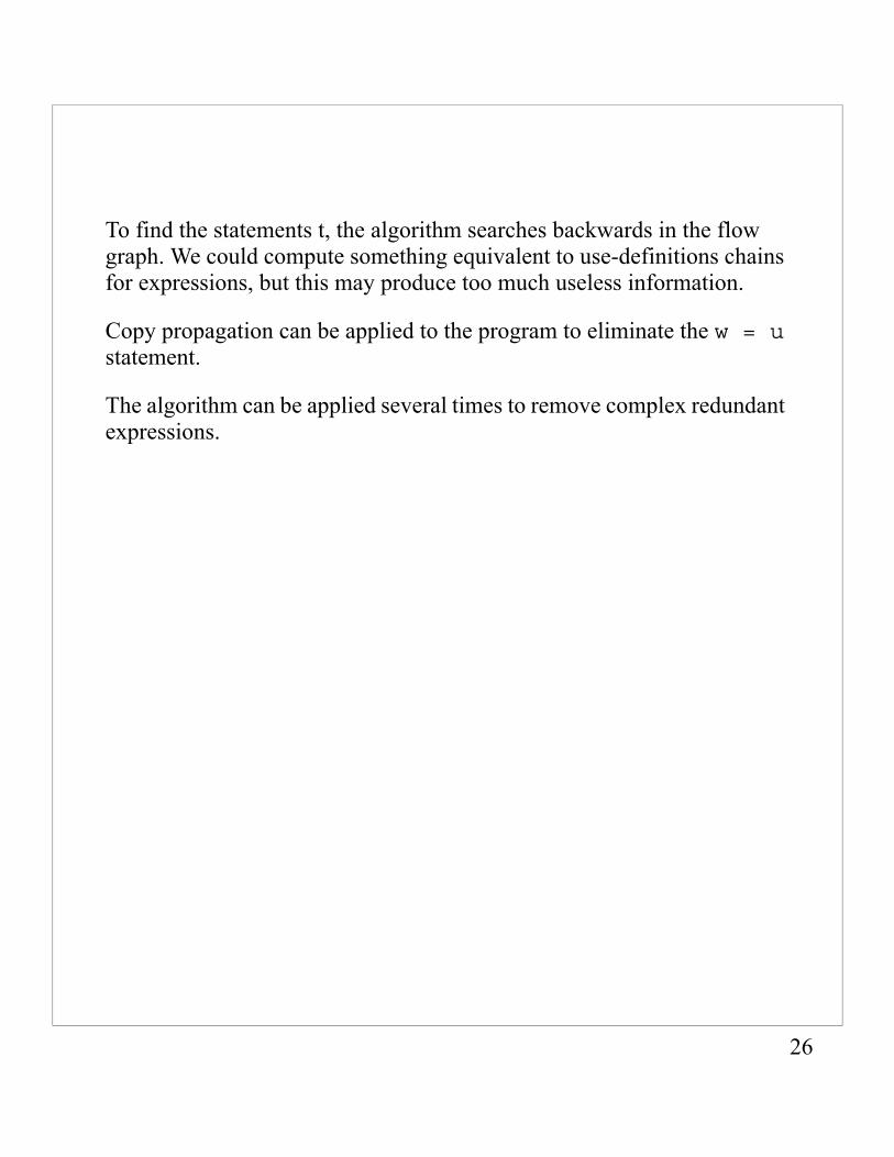
To find the statements t, the algorithm searches backwards in the flow graph. We could compute something equivalent to use-definitions chains for expressions, but this may produce too much useless information.

Copy propagation can be applied to the program to eliminate the w = u statement.

The algorithm can be applied several times to remove complex redundant expressions.

27

Copy propagation

To eliminate copy statements introduced by the previous algorithm we first need to solve a data flow analysis problem.

Let cin[B] be the set of copy statements that (1) dominate B, (2) reach B, and (3) their rhss are not rewritten before B.

out[B] is the same, but with respect to the end of B.

cgen[B] is the set of copy statements whose rhs’s and lhs’sare not rewritten before the end of B.

ckill[B] is the set of copy statements not in B whose rhs or lhs are rewritten in B.

We have the following equation:

cin B[ ] cgen C[ ] cin C[ ] ckill C[ ]–( )∪

C PRED B[ ]∈∩=

Here we assume that cin[S]=∅

Using the solution to this system of equations we can do copy propagation as follows:

28

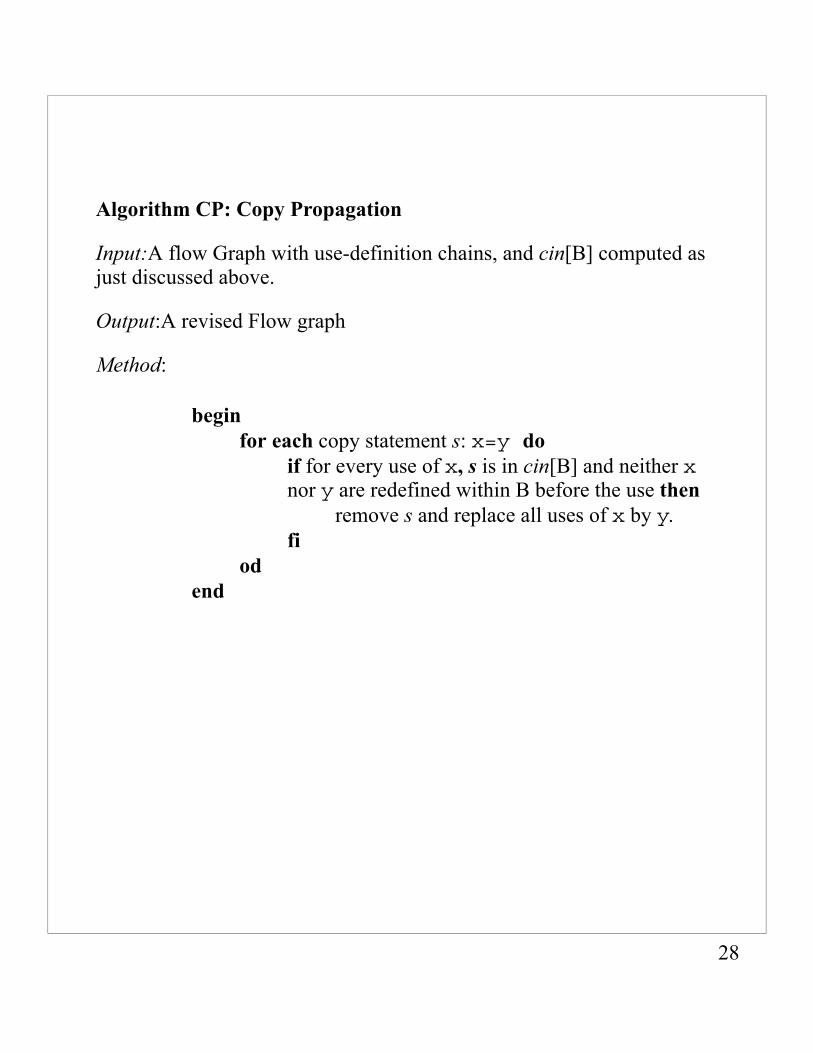
Algorithm CP: Copy Propagation

Input:A flow Graph with use-definition chains, and cin[B] computed as just discussed above.

Output:A revised Flow graph

Method:

beginfor each copy statement s: x=y do

if for every use of x, s is in cin[B] and neither x nor y are redefined within B before the use then

remove s and replace all uses of x by y.fi

odend

29

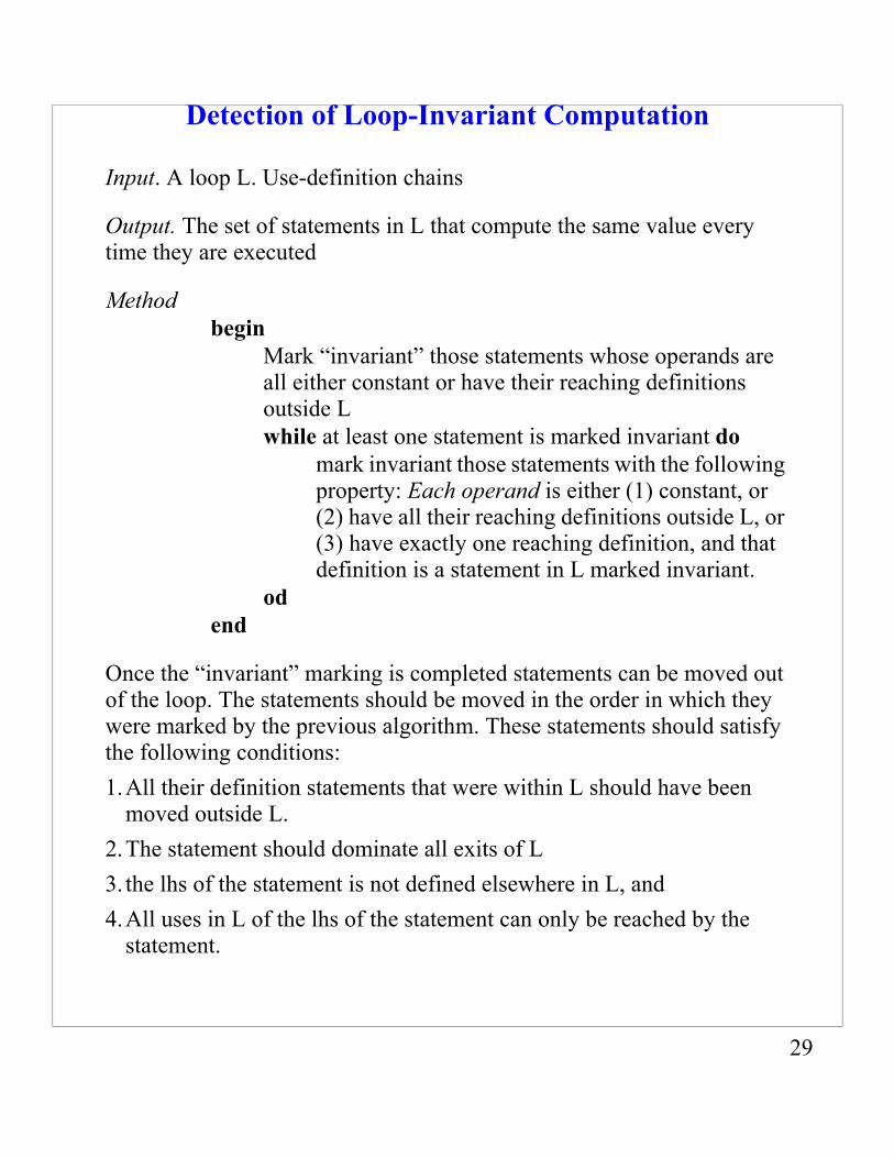
Detection of Loop-Invariant Computation

Input. A loop L. Use-definition chains

Output. The set of statements in L that compute the same value every time they are executed

Methodbegin

Mark “invariant” those statements whose operands are all either constant or have their reaching definitions outside Lwhile at least one statement is marked invariant do

mark invariant those statements with the following property: Each operand is either (1) constant, or (2) have all their reaching definitions outside L, or (3) have exactly one reaching definition, and that definition is a statement in L marked invariant.

odend

Once the “invariant” marking is completed statements can be moved out of the loop. The statements should be moved in the order in which they were marked by the previous algorithm. These statements should satisfy the following conditions:1.All their definition statements that were within L should have been

moved outside L.2.The statement should dominate all exits of L3. the lhs of the statement is not defined elsewhere in L, and4.All uses in L of the lhs of the statement can only be reached by the

statement.