Example 16.7 Forecasting Quarterly Sales at a Pharmaceutical Company

Example 16.7

Forecasting Quarterly Sales at a Pharmaceutical Company

Thomson/South-Western 2007 ©South-Western/Cengage Learning © 2009Practical Management Science, Revised 3eWinston/Albright

Pharmaceutical Sales.xlsx

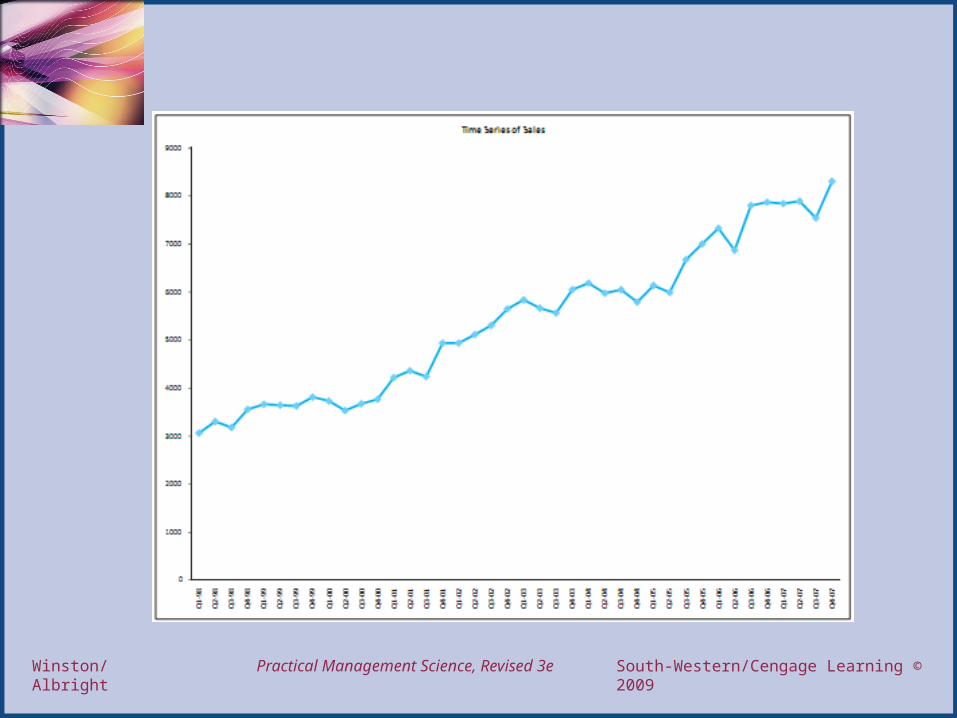
• This file contains quarterly sales data for a large pharmaceutical company from first quarter 1998 through fourth quarter 2007 (in millions of dollars).

• The time series plot shown on the next slide indicates a fairly consistent upward trend, with a relatively small amount of noise.

• Can Holt’s method be used to provide reasonably accurate forecasts of this series?



Solution

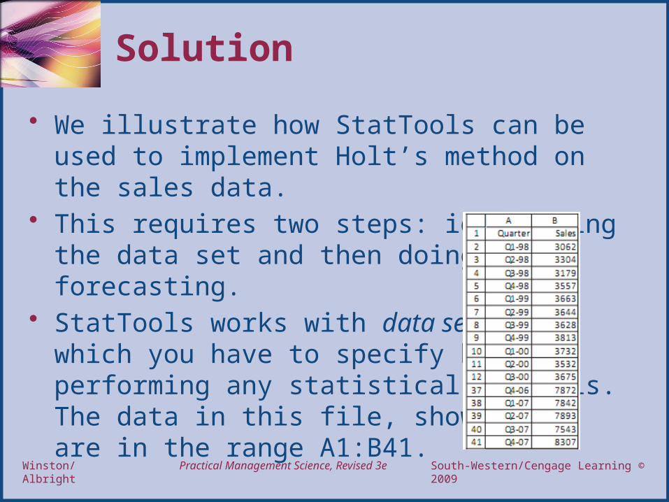
• We illustrate how StatTools can be used to implement Holt’s method on the sales data.

• This requires two steps: identifying the data set and then doing the forecasting.

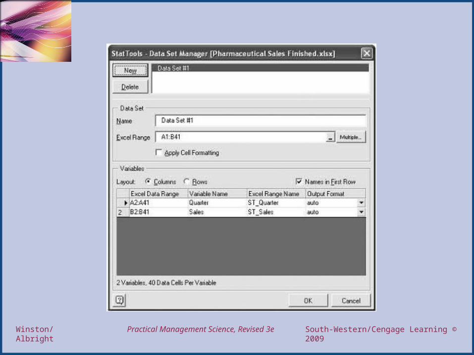
• StatTools works with data sets, which you have to specify before performing any statistical analysis. The data in this file, shown here, are in the range A1:B41.


Solution -- continued

• To specify the data set, select the StatTools/Data Set Manager menu item, fill out the resulting dialog box as shown on the next slide, and click on OK.

• Now you are ready to perform a statistical analysis on this data set.



Applying Holt’s Method to Forecast

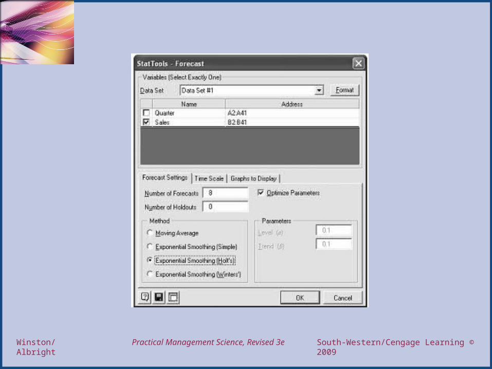
• To apply Holt’s method, select Forecast from the Time Series & Forecasting dropdown on the StatTools ribbon.

• There are three tabs on the resulting dialog box. The most important is the Forecast Settings tab, which you should fill in as shown on the next slide.

• This indicates that– Sales is the time series variable of interest– we want eight quarters of future forecasts– we are using Holt’s method,– we want to optimize the smoothing constants

• The other two tabs are straightforward and are not shown here.• The Time Scale tab lets you indicate that these are quarterly data,

beginning with quarter 1 of 1998, and the Graphs to Display tab lets you choose which of three graphs you want StatTools to create.



Discussion of the Results

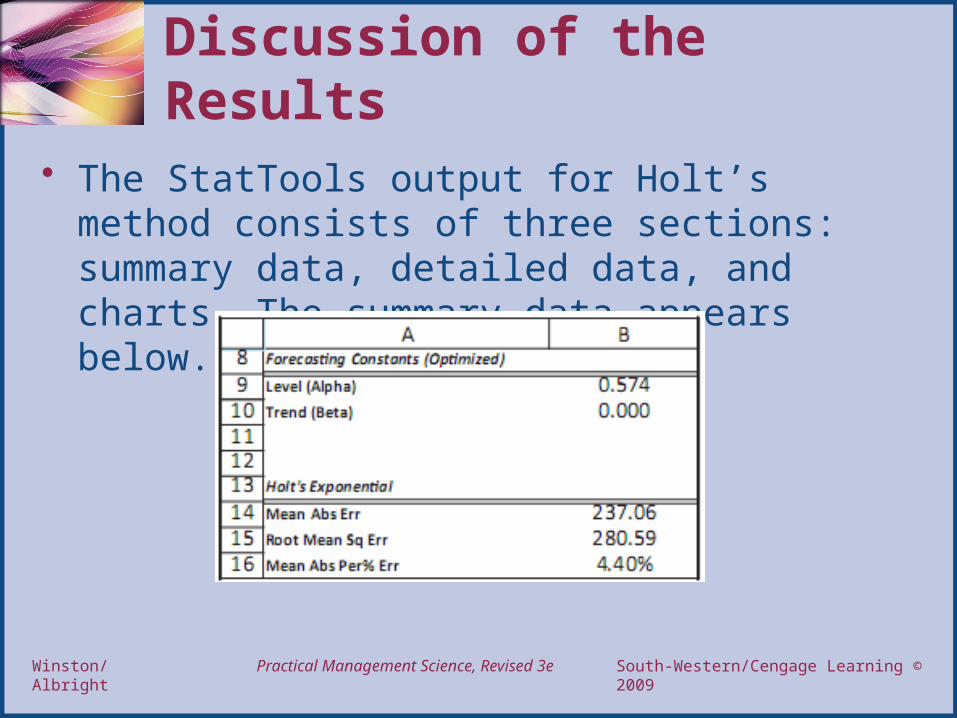
• The StatTools output for Holt’s method consists of three sections: summary data, detailed data, and charts. The summary data appears below.


Discussion of the Results -- continued

• They indicate that the best smoothing constants are 0.574 (for level) and 0.0 (for trend). These produce the error measures shown.

• For example, MAPE is 4.40%. Although the smoothing constants shown here minimize RMSE, you can experiment with other smoothing constants in cells B9 and B10.

• For example, if you set both smoothing constants equal to 0.2, you will see that RMSE increases to 349.54 and MAPE increases to 5.56%.

• Clearly, the choice of smoothing constants does make a difference.



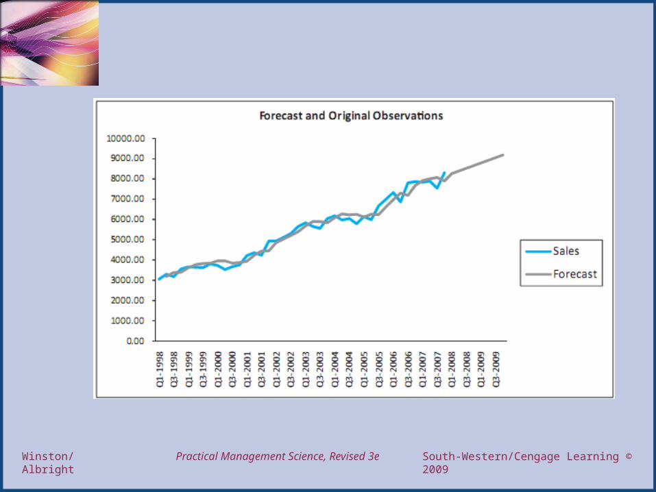
• Two useful charts produced by StatTools appear on the next two slides.

• The first of these superimposes the forecasts onto the original series. It also shows the projected forecasts at the right. We see that the forecasts track the series well, and the future projections follow the clear upward trend.

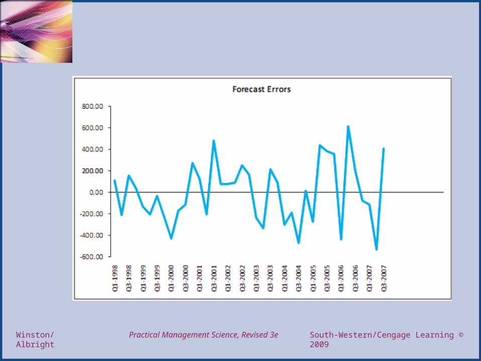
• The second shows the series of forecast errors. If the forecast method is working well, this chart should be “random,” with no apparent patterns. The only suspicious pattern evident here is that the zigzags appear to be increasing in magnitude through time.





• For our purposes, Holt’s method seems to be doing very well with this data set. It tracks the historical data closely, and it accurately projects the upward trend.

Documents

Example 16.7 Forecasting Quarterly Sales at a Pharmaceutical Company