Embed Size (px)
Citation preview

Examining Transmission Power in Minimum Capacity UnderwaterAcoustic Networks
by
Kathryn E.Stanchak
SUBMITTED TO THE DEPARTMENT OF MECHANICAL ENGINEERING INPARTIAL FULFILLMENT OF THE REQUIREMENTS FOR THE DEGREE OF
BACHELOR OF SCIENCE IN ENGINEERINGAS RECOMMENDED BY THE DEPARTMENT OF MECHANICAL ENGINEERING
AT THEMASSACHUSETTS INSTITUTE OF TECHNOLOGY ARCHES
FEBRUARY 2010
0 2009 Massachusetts Institute of TechnologyAll rights reserved
. l ) )-
OF TECHNOLOGv
JUN 3 0 2010
LIBRARIES
Signature of Author:DepaAment o echanical Engineering
December 18, 2009
Certified By:Franz Hover
Doherty Assistant Professor in Ocean UtilizationThesis Supervisor
Accepted By: .......John H. Lienhard V
--... ieomns rroiessor i Mvechanical EngineeringChairman, Undergraduate Thesis Committee
.... .......... . .......
Examining Transmission Power in Minimum Capacity UnderwaterAcoustic Networks
by
Kathryn E. Stanchak
Submitted to the Department of Mechanical Engineering onDecember 18, 2009 in Partial Fulfillment of the
Requirements for the Degree of Bachelor of Science inEngineering as Recommended by the
Department of Mechanical Engineering
ABSTRACT
This paper explores the prospect of reducing the transmission power required to operate linkswithin an underwater acoustic network by minimizing the total capacity of the network whilemaintaining certain data flow requirements. This is motivated by an approximate model forunderwater acoustic transmission power that demonstrates that decreasing the distance betweennodes, the capacity of a link between nodes, or both, reduces the power required to send a signalbetween those nodes. A procedure for determining a minimum-sum capacity network developedby Gomory and Hu in 1961 is applied to several common network topologies including tree,ring, and mesh structures. The approximate model for transmission power, which takes intoaccount the large effects of signal attenuation and noise, is used to evaluate these minimalnetworks.
The networks derived from the Gomory-Hu procedure are shown to require less totaltransmission power to operate the entire network. In order to maintain the pre-set data flowrequirements in the Gomory-Hu network, it is necessary to send information across multipleparallel paths in the network. Results show that because of this extra transmission distance, thenetworks derived via the Gomory-Hu procedure and their consequent parallel routing schemesare less efficient in terms of a single-transmission from one node to another node in the networkthan their counterpart networks that operate via a direct-access method, although thetransmission power requirements per node are reduced. This parallel routing scheme implies thatthe Gomory-Hu networks could be beneficial for multi-cast transmission. Results show thatapplying the Gomory-Hu procedure to networks intended for multi-cast instead of single-casttransmission could be a promising way of increasing the efficiency of the overall network.
Thesis Supervisor: Franz HoverTitle: Doherty Assistant Professor in Ocean Utilization

TABLE OF CONTENTS
Introduction ___ _ _.____ _ _.__ _. 4
Section 1: Graph Networks _._6.................. . ........................ 6
1.1: Flow Networks and the Max-Flow Min-Cut Theorem 6
1.2: Gomory-Hu Minimal Network and Prim's Algorithm 7
Section 2: The Underwater Acoustic Channel 13
2.1: Frequency Dependent Factors ...................................... 13
2. 1 Signal Attenuation .................................... ..... 13
2.1.2. Noise 13
2.2: Acoustic Channel Model _____.. 16
Section 3: Network Topologies and Routing Schemes 20
3.1: Direct-Link vs. Multi-hopping Transmission ........................... 20
3.2: Parallel Transmission _______...____.23
Section 4: Gomory-Hu Results _. ___. ___.... ___ 25
4.1: Tree Network 25
4.2: Ring, Spoke, and Rectangular Array Topologies 34
4.3: Mesh (Ad-hoc) Network Topologies....._.......____.................37
C onclusions _ _ _ _ _ _ _ _ __ _ __ _ _. __ _ .__ _ _ _ _. 42
Appendix (A) ........................................................... 44

Introduction
Underwater acoustic networks consist of sensor nodes that communicate with each other
wirelessly by sending acoustic pressure waves through the medium of sea water. The
applications for these networks include environmental monitoring, establishing communications
with underwater vehicles, and as positioning systems for underwater localization and navigation.
Setting up these underwater sensor networks is often a very challenging task. As the pressure
wave travels through the ocean water it can undergo severe signal attenuation and high levels of
noise, much more than its electromagnetic wave counterpart. This results in signal spreading that
can lead to reverberation and also contributes to a very limited bandwidth availability.
Designing and optimizing networks that require a minimum level of transmission power to
operate is an attractive problem for research because it is often extremely expensive to, for
instance, change a battery on a sensor network node located in the deep sea. The focus of this
paper is to analyze power usage in a number of different network layouts. This is done by first
defining the network mathematically and then developing a model for the transmission power
required to transmit underwater. It is found that transmission power increases with respect to
both increasing distance between the two communicating nodes and increasing capacity of that
particular link, or the number of bits per second that can be transmitted. Motivated by this
relationship, different ways of manipulating the distance and capacity of links in a network are
examined. A procedure for a minimal sum-capacity network developed by Gomory and Hu in
1961 is looked at in particular.
The paper is organized as follows: Section 1 covers the representation of flow networks as
graphs and outlines the Gomory-Hu minimal capacity network procedure. Section 2 develops a
closed-form model for the transmission power of a link between two nodes in an underwater
network as a function of distance and capacity. Section 3 describes some simple network

topologies and forms of routing schemes applied to underwater acoustic networks. Section 4
applies the Gomory-Hu procedure in particular to several sample networks that are common to
underwater applications. Section 5 concludes the paper and provides suggestions for further
investigation.

Section 1: Graph Networks
The data signal sent from one node to another in an underwater acoustic network can be thought
of and modeled as a "flow" of information between those nodes. The motivation behind this
section is to develop a way to represent flow networks mathematically, in order to compare them
and perform calculations on them.
1.1: Flow Networks and the Max-Flow Min-Cut Theorem
A flow network can be described in terms of graph theory as graph G (J E) where V is the set
of vertices in the graph and E is the set of edges. For Figure 1.1 shown below, V = {u v w x} and
E = t(u,v) (v, w) (w, x) (x, u)}. Each edge is assigned a capacity of c (u, v)0 ; this is the
weight of the edge for this application. A flow between two vertices is represented as
f(u,v) c(u,v) [1].
UG,(u,v)
V c2(vw)
x
Figure 1. 1: A flow network represented as graph G =(V E).
For this paper, only networks that can be represented as connected graphs will be considered.
This means that for every vertex v e V there is a path s -* v - t where s E v is the source of
the flow and t E v is the sink. The graph shown in Figure 1.1 is connected. A fully-connected
network refers to a network in which each node is capable of transmitting to every other node.
All of the networks looked at in this paper are assumed to be capable of fully-connected
transmission. It will also be assumed that each link in every example network presented is bi-
directional. This means that a flow that can be sent from a source node to a sink node in any of

these networks can also be sent in the opposite direction (from the "sink" to the "source").
A cut in the flow network is any partition of the vertices into two disjoint subsets. The weight of
the cut is the sum of the weights of the edges crossing the cut. For example, a cut of G = (VE) is
shown in Figure 1.2. In this case, the two disjoint subsets are V, = [u} and V2 = {v w x} and the
weight of the cut is the sum of c1 and c4.
Uc,(uYv
vc,(u,x)
c2(v'w)
x
C3(WX)W
Figure 1.2: Flow network G = (V E) cut into two disjoint subsets.
In 1956, Ford and Fulkerson devised an algorithm to compute the maximum flow in a network
from a single source to a single sink [2]. In doing so, they also proved the max-flow min-cut
theorem, which states that the maximum flow in a network from s -+ t is equal to the minimum
capacity cut such that s and t are in different partitions of V For c1 = C4 1 and c2 = C= 2, the cut
shown in Figure 1.2 is the minimum cut and its capacity weight, 2, is also the maximum flow
from u to any other vertex in the network.
1.2: Gomory-Hu Minimal Network and Prim's Algorithm
Gomory and Hu used the max-flow min-cut theorem in 1961 as their primary tool for developing
a synthesis procedure for a minimum capacity network [3] [4]. In their procedure, a minimum
capacity network is defined as the synthesized network in which the sum of the capacities in the
network is at a minimum while the network is still able to fulfill certain capacity requirements.
The idea essentially uses capacity as a cost for each link and the procedure seeks to minimize

this overall cost. The max-flow min-cut theorem is used to ensure that the capacity requirements
of the network are met while minimizing the total capacity.
The Gomory-Hu procedure begins with an initial network of vertices connected by links with
assigned capacities. These initial capacities dictate the flow requirements of the network. The
link capacity from one node connected directly to another node defines the total flow between
those nodes that must be maintained in the final network. An example network, N= (V E)
shown below in Figure 1.3 is used to demonstrate the Gomory-Hu procedure throughout this
section:
a 7 f7
b 12 6 104 10 g
C5 9 6 10
9
d 5 e '9 'h
Figure 1.3: Flow network N = (V E), initial network used in Gomory-Hu demonstration.
The dominant requirement tree referred to by Gomory and Hu is more familiarly known as a
maximum spanning tree. A maximum spanning tree of a graph is the tree with the largest sum of
edge weights that connects all of the vertices in the graph. Multiple algorithms have been
developed for determining a minimum spanning tree which can be easily altered for the problem
of a maximum spanning tree. In this application Prim's Algorithm [5] with the required alteration
for a maximum spanning tree was used. The implementation of Prim's Algorithm in Matlab used
in this paper is given in Appendix (A) with annotations. Figure 1.4 below shows a dominant
requirement tree highlighted for network N:

gC
9 109
d e
Figure 1.4: The dominant requirement tree for network N.
The next step in forming the minimal network is to partition the dominant requirement tree, T,
into a set of uniform trees U= [U ... U,}. The first uniform tree, U, contains the same edges as
T, but each edge has a capacity of c(u, v) = m, the minimum capacity in T. For the next tree, U2,
the edges in T of c(u, v) = m are deleted, and the uniform edge capacity is the min(c(u, v) - m).
These steps are continued to create a forest of uniform trees, all with edge capacities of c(u, v) >
0, as shown in Figure 1.5.1-3:
7 f
Figure 1.5.1: The first uniform tree, U1.
a f
3 3
9C
2 32
d 2 h
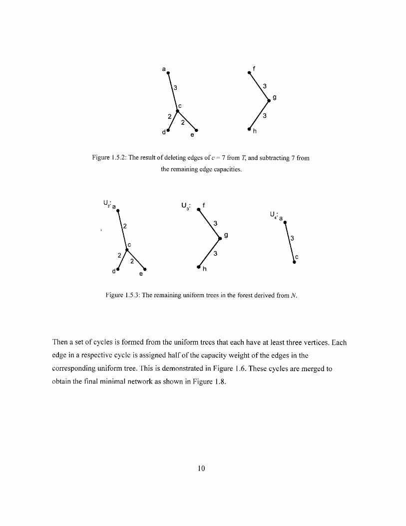
Figure 1.5.2: The result of deleting edges of c = 7 from T, and subtracting 7 from
the remaining edge capacities.
U2:
2
C
2
22
2d e
U : f
3
9
3
h
Figure 1.5.3: The remaining uniform trees in the forest derived from N.
Then a set of cycles is formed from the uniform trees that each have at least three vertices. Each
edge in a respective cycle is assigned half of the capacity weight of the edges in the
corresponding uniform tree. This is demonstrated in Figure 1.6. These cycles are merged to
obtain the final minimal network as shown in Figure 1.8.
U :4 a
3c

3.5 f
1.5
9
C4a
3
c
f
1.5
g
1.5
Figure 1.6: The set of cycles C = {C1, C2, C3, C4} form from the set of
uniform trees U derived from T
3.5
d 4.5 3.5 h
Figure 1.8: The final Gomory-Hu minimal network derived from N.
11

The cycles must be formed such that the minimum cut in the uniform tree is maintained to ensure
the final network meets the flow requirements of the dominant requirement tree. Following from
that, the minimum cut must not be increased when the cycle is formed to ensure that the final
network is indeed minimal. This requirement on cycle formation comes directly from the max-
flow min-cut theorem. There may be other solutions to the Gomory-Hu procedure for a particular
initial network because a maximum spanning tree of a graph is not necessarily unique and the
cycles made from the forest of uniform trees may be formulated in any way so long as the
minimum cut is maintained. It can be seen from this example that the Gomory-Hu procedure
takes away edges and adds others to the initial network layout. This is why it is important that
each node in the network is capable of transmitting to every other node, or in other words,
capable of fully-connected transmission. The algorithms written for this paper to complete the
steps involved in the Gomory-Hu minimal network procedure along with Prim's Algorithm are
implemented in the Matlab language in Appendix (A).

Section 2: Underwater Acoustic Channel
In order to analyze underwater acoustic sensor networks, it is important to determine the
fundamental capabilities of nodes communicating through the underwater acoustic channel. In
this section, a closed-form model of the transmission power required to send an acoustic signal
between two nodes in a network is developed. Also, the frequency dependent characteristics of
underwater acoustic transmission are explained in order to better understand these effects on the
final model.
2.1: Frequency Dependent Factors
Unlike communication signals sent within the electromagnetic spectrum, acoustic signals are
pressure waves and consequently they experience more frequency dependent distortion. This
distortion is due to signal path loss, or attenuation, as the acoustic wave propagates through sea
water and the ambient noise always present in deep sea waters. Because many of the problems in
designing feasible and efficient underwater acoustic networks are a result of this high level of
distortion, it is important to understand the contributing factors and to accurately characterize
them in any formulation of a channel model.
2.1.]: Signal Attenuation
The attenuation of an acoustic signal can be thought of as a result of two factors - the
geometrical spreading of the sound pressure wave and the absorption of some of the acoustic
energy [6]. This is modeled as:
A (l, f )(l/1,)k a (f
or, expressed in dB:
10 log (A (l, f ))=k 10 log (l/1,)+l 10 log (a (f))

where I is the distance over which the signal is transferred, bejis a reference distance, k is the
spreading factor, and a(f) is the absorption coefficient. The spreading factor, k, describes the
geometry of the propagating acoustic signal. A practical value that will be used here is k = 1.5,which corresponds to an average of spherical and cylindrical spreading. The absorption
coefficient models the acoustic energy that is transformed into heat as the signal propagates
through the channel [7]. It is actually a function of frequency, salinity, temperature, and
hydrostatic pressure, but an empirically determined formula useful for most practical frequency
ranges gives the absorption coefficient solely as a function of frequency:
100og (a(f))0. 11( 2)+44( 2 ) +2.75 x1I0-4f2+ 0.0031+f 4100+f 2
for a(f) expressed in dB/km andf in kHz. The absorption coefficient is shown in Figure 2.1:
350
300
- 250
1200
0 200 400 600 800 1000frequency [kHz]
Figure 2.1: The absorption coefficient a(f) from Eq. (2.3).

2.1.2. Noise
The acoustic signal is also affected by the deep sea ambient noise level. The dominant sources
that contribute to the overall noise level are turbulence, shipping, surface agitation caused by
wind, and thermal noise primarily caused by sea motion on a molecular scale. The overall noise
level can be determined as a sum of the noise caused by each of these sources, according to these
empirical formulae [8]:
N,=17-30 loglo(f)
N= 40+20(s-0.5)+261ogl0 (f)-60 log 0 (f+0.03)
N,=50+7.5w "+20 loglo(f)-401og1 (f+0.4)
N,1=- 15+20 log 10(f )
N=l0logio(1ON,/l110 N,/10 0 N /10 IN,,110)
where N,, N, N, and Nh are the noise spectrum levels due to turbulence, shipping activity, wind,
and thermal noise and N is the overall noise spectrum level. The shipping density constant, s, is
measured on a scale from 0, meaning very light shipping activity, to 1, heavy shipping activity.
The wind speed, w, is measured in m/s. Figure 2.2 shows the noise spectrum level for various
amounts of shipping activity and different sea states. In this figure it is evident that different
noise sources predominate in different frequency decades.

110
100- --
90
(LE 8S---o
70
60 -..-
E50 -. ..
40--
0 -S
2010~3 10-2 10-1 10o 10' 102 10,
frequency [kHz]
Figure 2.2: The ambient noise spectrum levels for various sea states and levels of shipping
activity. In the frequency range of 10.2 to 10- the shipping activity has the greatest
effect on the noise spectrum level and is plotted at s = 0, s = 0.5, and s = 1, from
top to bottom. In the frequency range of 10- to 10', wind speed has the greatest
effect on the noise spectrum level and is plotted at w = 14 m/s, w = 8 m/s,
w = 3 m/s, and w = 0 m/s, from top to bottom.
2.2: Acoustic Channel Model
An approximate model can be obtained via a numerical procedure to provide a more reasonable
way of evaluating these parameters for the purposes of network analysis. The model found in [9]
and used in this paper is computed for two ranges of (l, C):
Range 1: lE[0,l0]km,CE[02]kbps
Range2: lE[0100]km,C E[0,100]kbps
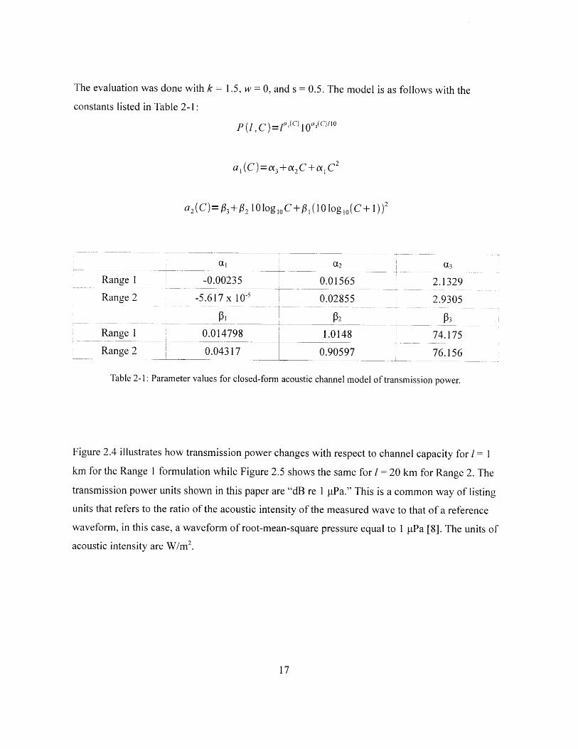
The evaluation was done with k = 1.5, w = 0, and s = 0.5. The model is as follows with the
constants listed in Table 2-1:
P (1, C) =l a(C) 10/n
aI (C)=ax3+ 2C+a 1 C2
a 2(C)=#3+# 2 10log 10C+p 1 (10 log 1O(C+ 1))2
Range 1
Range 2
Range 1
Range 2
(X1
-0.00235
-5.617 x 10⁻⁵
0.014798
0.043 17
U2
0.01565
0.02855
P2
1.0148
0.90597
QX3
2.1329
2.9305
P374.175
76.156
Table 2-1: Parameter values for closed-form acoustic channel model of transmission power.
Figure 2.4 illustrates how transmission power changes with respect to channel capacity for /= 1
km for the Range I formulation while Figure 2.5 shows the same for /= 20 km for Range 2. The
transmission power units shown in this paper are "dB re 1 jPa." This is a common way of listing
units that refers to the ratio of the acoustic intensity of the measured wave to that of a reference
waveform, in this case, a waveform of root-mean-square pressure equal to I pPa [8]. The units of
acoustic intensity are W/m 2 .

0'5 1n0.5 1 1
Capacity [kbps]
Figure 2.4: P(l, C) for /= 1 km.
0 5 10 15 20Capacity [kbps]
Figure 2.5: P(l, C) for I = 20 km.
18
135
130-
0
-. .. ..- .

Figures 2.4 and 2.5 show that power increases quite a bit as the available capacity of the channel
is increased, which intuitively makes sense. It does the same with respect to increasing
transmission distance. This indicates that the relationship between transmission power, distance,
and capacity can be utilized to optimize underwater acoustic networks or at least to come up with
some reasonable design guidelines. The following sections of the paper suggest different ways of
manipulating these parameters in order to maximize power efficiency in underwater acoustic
sensor networks.

Section 3: Network Topologies and Routing Schemes
The problem this paper is focusing on essentially concerns evaluating underwater network
topologies and routing schemes. The routing scheme of a network is the method used to find a
path over which information is directed through the network from a source node to a sink node,
which may result in transmitting through intermediate nodes. The topology of a network refers to
the physical layout of the nodes in space. Because the transmission power of an acoustic signal
depends so heavily on distance, there have been several relatively simple analyses done to
examine optimal placements of nodes within a network. While it is difficult to come up with a
generalized case because there are many factors that go into planning an acoustic network layout,
such as the size of the area that needs to be monitored by the sensors, the cost of adding
individual additional nodes to the network, and the characteristics of the sea water and/or the
ocean floor at the suggested site, there are some basic guidelines useful for network synthesis
provided by the relationship between power, capacity, and distance.
3.1: Direct-Link vs. Multi-hopping Transmission
A direct-link between two nodes in a network is defined as the straight-line path between those
nodes that does not transmit through any intermediate nodes. It is the simplest case to consider.
An example is shown in Figure 3.1:
a ,C x
Figure 3. 1: A direct-link between node a and node x over a distance I with
a channel capacity of C.

A method known as "multi-hopping" divides the distance between two nodes so that the signal is
transmitted through several intermediate nodes on its way from the source node to the sink node
[10]. In this way, the transmission "hops" along multiple shorter distances instead of following
one longer direct-link path. The direct link example is modified in Figure 3.2 for N= 3, where N
is the number of hops from the source to the sink:
b I/3, C c I/3, C
Figure 3.2: An example of a transmission link via multi-hopping.
Power usage for multi-link networks can be calculated as follows:N
P,=Z Pi
where P, is the total transmission power, N is the number of hops in the network, and P is
transmission power as defined by the model in Section 2.
To compare direct-link transmission with the method of multi-hopping, the total transmission
power needed for sending over a distance / is calculated N= 1 to 25 hops over that distance. For
this case, the above equation simply becomes:
P=N P( ,C)N
a- I/3, C x

The case of N= I is the direct-link transmission from the source node to the sink node. For the
examples distances used in this simulation, the transmission power model formulation for Range
I is used. The results are shown in Figure 3.3:
190
180
0 10 15N [number of nodes]
20 25
Figure 3.3: Total transmission power for a multi-hop routing scheme for various numbers
of nodes. From top to bottom: / = 100km, C = 5 kbps; I = 50, C = 5 kbps;
l= OOkm, C= I kbps; I = 50 km, C= I kbps.
Figure 3.3 easily demonstrates that a network topology and routing scheme based on multi-
hopping is more efficient than transmitting directly from the source node to the sink. It also
indicates that reducing the capacity of the underwater channel transmission adds to this effect.
-a

3.2: Parallel Transmission
Another network topology and routing method to consider is that of parallel transmission. In
parallel transmission, a signal is sent through multiple paths from the source node to the sink. An
example is shown in Figure 3.4:
a X
Figure 3.4: Parallel routing scheme: sending information along two paths from a --+ x.
In this example, if the capacities of the parallel links are each the same as the capacity in the
direct link, and the distance between a and x is also the same, the transmission time needed to
send an equivalent amount of data from the source to the sink is halved: t(,rareIs= tdic,/2 . Since the
power requirements for all of the links are the same (because the distances and capacities are the
same), the total power is simply doubled in the parallel network; however, since the transmission
time is cut in half, the overall energy usage stays the same. This suggests that parallel routing
schemes could be used to reduce transmission times without having too much of an effect on the
amount of energy required to complete the transmission. It is necessary to transmit over parallel
paths in a Gomory-Hu network in order to achieve the transmission data rates established by the
dominant requirement tree.
For the purposes of parallel transmission it will be assumed that the nodes in a network can
simultaneously send data to multiple nodes and simultaneously receive data from multiple nodes
using established multiple access methods. These techniques include Frequency Division
Multiple Access (FDMA), Time Division Multiple Access (TDMA), and Code Division Multiple
Access (CDMA). FDMA assigns different frequency bands to transmit in to different nodes.

Reference [9] has a minor result that shows for low capacities, the optimal frequency at which to
transmit varies greatly for different transmission distances, indicating that FDMA is a promising
technique in these sorts of underwater acoustic networks. In TDMA, each node occupies a
different time slot. The time slots repeatedly cycle. Because of signal attenuation and the long
delay inherent in the underwater channel, TDMA is typically not the best multiple-access option.
In CDMA, the signal is multiplied by a pseudonoise code sequence that can be decoded by the
receiving node. If the code sequences used by the different nodes are orthogonal to each other,
then they can transmit at the same time within the same frequency band. The receiver will only
detect the intended signal because the others will appear as noise due to decorrelation [II].
CDMA techniques are a viable option for underwater acoustic communications.

Section 4: Gomory-Hu Results
The Gomory-Hu network synthesis procedure reduces an existing network topology to the
topology with minimum-sum of network link capacities. The motivation behind reducing link
capacity as a means for reducing transmission power requirements can be seen in Figures 2.4 and
2.5 in Section 2, which show that transmission power requirements increase as the channel
capacity increases. Because the Gomory-Hu procedure is applied on the scale of the entire
network instead of merely analyzing individual links in a network one-by-one, it is difficult to
develop a general case for the purposes of optimization. Here results are shown for a sampling of
different network topologies to get a feel for how networks synthesized via the Gomory-Hu
procedure behave differently from networks that operate by a traditional direct-link transmission
method. Examples are shown for various common network topologies, including tree, ring, and
ad-hoc networks, as well as for networks of different node densities and with different ranges of
capacity values.
4.1: Tree Network
A tree network, or a hierarchical network, consists of several nodes of different "levels,"
beginning with a root node at the top of the tree that usually serves as the central information
junction, the beginning and end of most transmissions to and from other nodes. A tree is
acyclical. In a tree there is at most one simple path from one node to any of the other nodes,
which means that there is one path from one node to any of the other nodes without retracing any
of the vertices within the path. Changing a tree structure to a Gomory-Hu network, which is
cyclical by nature (cycles are created within the procedure itself), creates multiple simple paths
between one node and any of the other nodes.

To illustrate the effects of applying the Gomory-Hu procedure to tree networks, the trees shown
in Figure 4.1 will be used as examples. Tree 1 is plotted on a grid with markings 10 km apart
with capacities ranging from 10 to 3 kbps so the model for channel power for Range 2 is used.
Tree 2 is plotted at 1/10 the scale of Tree 1 (the grid is set at 1 km), and the capacities range from
1 to 0.3 so the model for Range 1 is used to calculate power.
Tree 1: Tree 2:
Figure 4.1: Example tree networks to illustrate the effects of the Gomory-Hu procedure.
Tree 1 is plotted on a scale of 10 km while Tree 2 is plotted on a scale of 1 km.

Tables 4-1 and 4-2 list the the amount of power necessary to transmit along each of the links in
Tree I and Tree 2, respectively. Distance refers to the distance between each node in the link.
Distance (km) Capacity
28.28 10
28.28 10
28.28 5
28.28 5
28.28 5
20 5
Link
A <+B
A <+C
B <+D
B <+E
C ++F
D <+I
E <+J
E +-K
F +-G
F <+H
3
3
(kbps) Power [dB re I pPa]
196.50
196.50
189.69
189.69
189.69
185.07
181.28
185.81
185.81
181.28
Table 4-1: Link transmission characteristics for Tree I shown in Figure 4.1.
Distance (km)
2.83
2.83
2.83
2.83
2.83
2
2
2.83
2.83
2
Capacity (kbps) Power [dB re I pPa]
1 144
144
0.5 140.83
0.5 140.83
0.5 140.83
0.5 137.61
0.3 135.32
0.3 138.54
0.3 138.54
0.3 135.32
Table 4-2: Link transmission characteristics for Tree 2 shown in Figure 4.1.
20
28.28
28.28
20
Link
A <+B
A ++C
B +-D
B <+E
C <+F
D ++I
E <+J
E<+K
F <+G

Applying the Gomory-Hu procedure results in the network topologies shown in Figure 4.2. The
network result using Tree 1 is labeled G-H Network 1 and the result from using Tree 2 is labeled
G-H Network 2. The respective scales of the networks are the same as their corresponding trees
in Figure 4.1.
G-H Network 1:
1.5
G-H Network 2:
1.5 G 1.5 0.15 0.15 G 0.15
Figure 4.2: The results of the Gomory-Hu procedure applied to the example trees shown
in Figure 4.1. G-H Network 1 is derived from Tree 1, and G-H Network 2 is
derived from Tree 2.
F
0.15
H

Like the calculations presented for the tree networks, the amount of power necessary to transmit
along each of the links in G-H Network 1 and G-H Network 2 is presented in Tables 4-3 and 4-4:
Distance (km) Capacity
28.28 5
28.28 5
40 2.5
28.28 2.5
28.28 2.5
40
20 1.5
20 2.5
28.28 1.5
44.72 1
20 1.5
20 1.5
20 1.5
20 1.5
(kbps) Power [dB re I [tPa]
189.69
189.69
189.13
184.61
184.61
183.95
177.12
180.09
181.59
185.39
177.12
177.12
177.12
177.12
Table 4-3: Link transmission characteristics for G-H Network I shown in Figure 4.2.
Link
A <>B
A <+C
B <+C
B <+E
C <+F
E <+D
E ++J
D <+I
D <>K
F <- I1
F <+H
F <+G
G -+I
J <-+ K

Link Distance (km) Capacity (kbps) Power [dB re 1 pPa]
A B 2.83 0.5 140.83
A+-+C 2.83 0.5 140.83
B -+ C 4 0.25 140.94
B +-+ E 2.83 0.25 137.73
C <-+ F 2.83 0.25 137.73
E +-+ D 4 0.1 136.89
E + J 2 0.15 132.25
D <->- 2 0.25 134.51
D K 2.83 0.15 135.47
F < 4.47 0.1 137.91
F H 2 0.15 132.25
F G 2 0.15 132.25
G - 2 0.15 132.25
J K 2 0.15 132.25
Table 4-4: Link transmission characteristics for G-H Network 2 shown in Figure 4.2.
Adding the transmission power for each of the links in a network will give the total power
required to transmit through the entire network. The correct way to add power listed in dB is
shown below:
a dB + b dB = c dB
where
c =10 log 10 (10""+ 10b10)

The total power required to transmit through each of the networks is shown in Table 4-5:
Network Total Power [dB re 1 pPa]
Tree 1 201.17
G-H Network 1 196.39
Tree 2 150.44
G-H Network 2 148.71
Table 4-5: Comparison of power required to transmit over the entire network
for Tree 1, Tree 2, and their derived Gomory-Hu networks.
The results posted above do not necessarily represent a fair comparison between the trees and
their corresponding minimal networks. One of the main ideas behind the Gomory-Hu procedure
is to maintain the flow requirements of the initial network, which is not the case in the
calculations done for Table 4-5. For example, the link B +-* E is present in both Tree I and G-H
Network 1. It makes sense that the power required to operate that link in G-H Network 1 was
reduced from that required in Tree I because the link capacity was decreased, and therefore
transmits less information in the same amount of time. Although Table 4-5 shows reduced power
requirements for the G-H Networks, those networks will transmit less total data than the original
Trees over the same transmission duration.
In order to maintain the information flow requirements presented in Tree 1, information needs to
be routed through parallel paths in G-H Network 1. The paths needed for the B -+ E
transmission example are shown in Figure 4.4. The Tree 1 capacity of 5 kbps is sent directly
from B -- E. In the resultant Gomory-Hu minimal network, one routing method is to transmit at
2.5 kbps directly from B -+ E while transmitting 2.5 kbps along another path that traverses nodes
C, E, F, G, H, I, J, and K to E. The links used for each respective communication scheme are
highlighted in Figure 4.3:

Tree: Gomory-Hu:
A A
10 10 5 5
B C B 2.5 C
5 5 5 2.5 2.5
E D F E 1 D F
3 1.53 5 3 3 1.5 2.5 1 1.5
KG 1. 1.5 G 1.5 H
Figure 4.3: The paths over which a signal from B -+ E traverses in the Tree I scheme and the
Gomory-Hu scheme.
The total power necessary for transmitting from B <-+ E in the Tree is 189.69 dB (re 1 pPa),
while the total power necessary for transmitting in the Gomory-Hu scheme is 193.97 dB (re 1
VtPa). In comparisons of single transmissions, the Gomory-Hu network is more inefficient with
respect to the total power used by the network. This is most likely due to the large amount of
extra distance the signal needs to traverse to maintain the capacity requirements. However, this
193.97 dB (re I tPa) is spread amongst multiple nodes. No single node in this Gomory-Hu
transmission requires the power necessary for node B to transmit to E directly.
There are several observations to take away from this analysis. The first is that reducing the sum
of the network capacities does decrease the power required to transmit with the entire network
on," which is expected according to the channel model. When considered in terms of individual
signal transfers between a single source node and a single sink, the Gomory-Hu derived network
is more inefficient most likely because the overall distance the signal travels, in this case, is
much greater. One thing to notice is that the routing scheme naturally suggested by the Gomory-
Hu procedure inherently transmits the same information to multiple nodes even if it is only

intended for a single sink node. This suggests that although from a single-source, single-sink
point of view the Gomory-Hu network appears to be less efficient than direct-access routing
schemes, it might have applications in multi-cast transmission, which is the problem of sending
data from a single source to multiple sink nodes.
An example for multi-cast transmission can be shown for these tree networks. If we suppose that
node A wants to transmit the same information to all of the other nodes in the network at the
rates specified by Tree I and Tree 2 respectively, then for Tree I this is equivalent to transmitting
through each link in the network (although not simultaneously) and for Tree 2 it is equivalent to
leaving the entire network "on," because the Gomory-Hu network inherently involves
simultaneous transmission. In sending say, from A to B, every node in the network is already
activated. The results shown above for the amount of transmission power required to operate all
of the links in the networks indicate that the Gomory-Hu network is more efficient in this case.
This demonstrates that the option of building a network according to the Gomory-Hu procedure
should be explored if the network is intended for multi-cast transmission. The actual amount of
savings the Gomory-Hu network provides depends on the how the multi-cast information is
coded to reach its destination nodes.
One strictly topological benefit of using a Gomory-Hu derived network instead of the initial tree
is that a Gomory-Hu network will always contain cycles. In a tree network, if one link is lost, the
result is that at least one node, if not several, are completely cut off from the rest of the network.
In any Gomory-Hu network, there are multiple paths leading to and out from every node in the
network, helping to protect the nodes from being stranded due to some sort of system failure.

4.2: Ring and Spoke Topologies
In a ring network, each node in the network connects to two, and only two, other nodes. There
are two paths from one node any of the other nodes in the network- "clockwise" around the ring,
or "counter-clockwise." Ring network topologies are especially important to consider in context
of the Gomory-Hu minimal network, because the Gomory-Hu synthesis procedure creates a
network that is essentially the result of combining several cycles. This means that every Gomory-
Hu network is cyclical; it contains cycles, or "rings." A spoke network is most commonly set up
as a central node, or hub, that transmits and receives information from the other nodes distributed
around it, which are connected like spokes. Ring networks are especially important to consider
with respect to spoke networks as well, since for a spoke network in which all the links are of
equal capacity, the resulting Gomory-Hu network is simply a cycle with link capacities exactly
half of those in the original topology. Figure 4.4 demonstrates the transformation of a spoke
network into a ring network via the Gomory-Hu procedure.
1 1 0.5 0.5 0.510.5
1 0.5 0.51
0.5
Figure 4.4: Transformation of a spoke-topology network into a ring network according to the
Gomory-Hu procedure.
Rings also provide a regular example that can be used to evaluate Gomory-Hu networks. The
number of nodes in a ring can be increased in a relatively regular fashion like the points and
sides in regular polygons. Figure 4.7 shows rings networks that take the shape of regular
polygons with various numbers of sides, N.
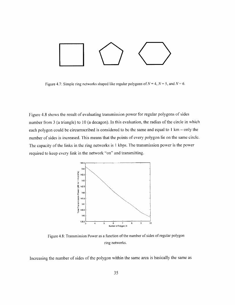
Figure 4.7: Simple ring networks shaped like regular polygons of N = 4, N = 5, and N = 6.
Figure 4.8 shows the result of evaluating transmission power for regular polygons of sides
number from 3 (a triangle) to 10 (a decagon). In this evaluation, the radius of the circle in which
each polygon could be circumscribed is considered to be the same and equal to 1 km - only the
number of sides is increased. This means that the points of every polygon lie on the same circle.
The capacity of the links in the ring networks is I kbps. The transmission power is the power
required to keep every link in the network "on" and transmitting.
144
143.5
143
> 141.50
E141
5 140.5
140
139.53 4 5 6 7
Number of Polygon, N8 9 10
Figure 4.8: Transmission Power as a function of the number of sides
ring networks.
of regular polygon
Increasing the number of sides of the polygon within the same area is basically the same as
N'N

increasing the number of nodes in a path, or multi-hopping. Figure 4.8 demonstrates that rings
with more nodes benefit from the effects of multi-hopping. This indicates that applying the
Gomory-Hu network synthesis procedure to spoke networks of high node density (resulting in a
ring that contains many sides) would have the most effect on power efficiency. Since Gomory-
Hu inevitably involves transmitting along parallel paths over a greater total distance, these
synthesized networks can greatly benefit from the effects of multi-hopping and it seems possible
that this procedure is most effective in situations with a high node density. This is different from
the multi-cast savings shown for Tree I in Section 4.1, which could have benefited by having
higher initial capacities than Tree 2, which demonstrated a greater node density. Combining these
two features seems to be the best way to utilize the Gomory-Hu procedure.
In a ring network, there are 2 paths to every node so the if one link fails there is still a way to
reach every other node. However, if another link were to fail this could completely cut off an
entire portion of the network. Spoke networks have the added safety measure of being able to
effectively isolate broken nodes and still transmit reasonably to the other nodes in the network.
The possibility of severe damage when these spoke are changed into rings increases as the
number of nodes in the ring increases. With more nodes in the ring there is a greater chance that
a large portion of the network could be cut off completely.

4.3: Mesh (Ad-hoc) Network Topologies
The organized network layouts studied in the previous examples of this section (tree, ring, spoke)
are useful for accessing the particular pros and cons of applying the Gomory-Hu procedure to
underwater acoustic networks. They also demonstrate the different criteria that can be used to
judge the Gomory-Hu networks against the original topologies. In contrast, this section will
cover the more general topic of the average performance of several networks with arbitrarily
placed nodes (or at least, nodes that are not placed and connected according to any regular
pattern). This type of seemingly random network layout is called a mesh, or ad-hoc, network. It
is a common network topology in wireless networks because the locations of wireless network
nodes are not constrained by the cost of installing a physical link. In this way, node locations can
be optimized according to other criteria. Mesh networks are also inherently the topology of
mobile wireless networks since networks comprised of mobile links can find themselves in any
number of configurations at any given time. While the Gomory-Hu procedure in the way it is
applied in this paper does not directly apply to mobile networks, those networks can be
considered as a stationary mesh network for any given moment in time for the purposes of
routing.
Four examples of mesh networks that are used in the demonstrations in this section are shown
below in Figure 4.9:

Mesh Network 1:
Mesh Network 3: Mesh Network 4:
Figure 4.9: Mesh network examples. The dominant requirement tree used to derive
Gomory-Hu minimal networks is highlighted in each tree.
The four examples of mesh networks shown in Figure 4.9 are used in this section to further
explore the application of the Gomory-Hu minimal network procedure. The total network
transmission power is evaluated for both the initial mesh network version and the minimal
network version of 12 different networks. Each initial network has 7 nodes and 11 links, in order
to keep the comparison as true as possible. The 12 networks consist of the above mesh network
examples applied to different scales. Group I consists of the four mesh networks plotted on a 0.1
km grid (grid as shown in the figures) for capacity values between 0 kbps and 2 kbps. The
constant values for Range I are used when evaluating transmission power according to the model
Mesh Network 2:

in Section 2. Group 2 consists of the four mesh networks plotted on a 1 km grid for capacity
values between 0 kbps and 2 kbps. The constant values for Range 1 are also used for Group 2.
Group 3 consists of the four mesh networks plotted on a 10 km grid with link capacity values
between 0 kbps and 20 kbps. For Group 3, the transmission power model constant values for
Range 2 are used.
Figure 4.10 shows the resultant Gomory-Hu minimal networks formed from the mesh networks
presented in Figure 4.7. Notably, the Gomory-Hu formulation for Network 2 is a ring, as is
common for networks with all or several link capacities of equal value. The Gomory-Hu Mesh
Network 2 also illustrates that it is not a requirement of Gomory-Hu networks that the listed
capacity into a node equals the listed flow out of a node. The Gomory-Hu network only shows
what each link itself needs to be capable of transmitting. For instance, in G-H Mesh Network 2
the link connecting a to g must be capable of transmitting at 1.5 kbps, but once that signal gets to
node g, it does not need to be passed on at the same rate to the other nodes downstream of it. G-
H Mesh Network 3 illustrates some of the layout difficulties with this procedure in that it is
difficult to write an algorithm that forms the minimal network links in convenient places relative
to the physical network. This problem only increases with the number of nodes in the network.
G-H Mesh Network 1: G-H Mesh Network 2:C
ad0.75
0..5
0.75 b050.
0.4 0.2 d
e 1.5 cb
0.1 0.2 0.5
0.25 d 0.5
0.35 e
f 0.25
g 0.5

G-H Mesh Network 3:
0.15 04 C
c 1.4 0.20.25 0.5
0.10.5
0.5 0.5 d 0.7b' ; 0.5 0.5
0.5O.4 0.25f0. 05
a- 0.25 -
Figure 4.10: The resultant Gomory-Hu networks from the example mesh networks
shown in Figure 4.7
Tables 4-6, 4-7, and 4-8 below list the transmission power comparisons for Groups 1 to 3,
respectively. Transmission power is listed in [dB re ptPa] according to the units described in
Section 2. The power is calculated as the amount of power necessary to transmit along every link
it the network. It should be kept in mind that although power usage appears lower for the
network, the Gomory-Hu network will need to transmit for a longer period of time and therefore
use more energy. This method of calculating transmission is power is used to see how consistent
the Gomory-Hu procedure is among similar networks (in terms of power calculations) and to
investigate the possibility that Gomory-Hu networks act differently according to their scaling in
terms of node density.
Network Number Power for Initial Mesh Network Power for Gomory-Hu Network
142.23 132.52
2 154.43 145.84
3 150.29 135.76
4 147.47 136.38
Table 4-6: Comparing total transmission power needed to operate the example mesh networks and
their corresponding Gomory-Hu minimal networks for Group I (scale of 0.1 km; 0 kbps < C < 2kbps).
G-H Mesh Network 4:

Power for Initial Mesh Network
164.83
175.97
171.79
168.95
Power for Gomory-Hu Network
153.93
167.34
157.16
157.79
Table 4-7: Comparing total transmission power needed to operate the example mesh networks and
their corresponding Gomory-Hu minimal networks for Group 2 (scale of 1 km; 0 kbps < C <2kbps).
Network Number
2
3
4
Power for Initial Mesh Network
206.37
217.55
217.11
213.83
Power for Gomory-Hu Network
208.81
210.69
206.89
205.62
Table 4-8: Comparing total transmission power needed to operate the example mesh networks and
their corresponding Gomory-Hu minimal networks for Group 3 (scale of 10 km; 0 kbps < C <20kbps).
As expected, since the sum of link capacities was reduced for each network, the sum of the
necessary transmission power levels associated with each link was reduced in the Gomory-Hu
minimal networks. Taking the proper scaling into account (since power is expressed in dB), there
doesn't appear to be much of a difference between the different node densities in the change in
power from the initial mesh network to the minimal network, based on these examples. The
results are consistent, with no network standing out as requiring drastically more or less
transmission power compared to similar networks.
Network Number

Conclusions
This paper shows that there are certainly some cases for which it is worthwhile to review the use
of the Gomory-Hu procedure for power efficiency. Sections 4.1 and 4.3 show that a Gomory-Hu
network uses less power in general to run the entire network (less power to keep the network
"6on"). This is because the model for transmission power shown as a function of distance and
capacity in Section 2 demonstrates that the transmission power required to operate links in a
network is reduced if the capacity of those links is reduced. However, in order to maintain the
same capacity requirements as the networks they are derived from, transmissions in Gomory-Hu
networks need to travel down multiple parallel paths. This increases the overall transmission
distance which in turn increases the amount of power needed to complete a single-source, single-
sink transmission. This increase in transmission distance appears to make the Gomory-Hu
network less efficient than the network it is derived from in terms of single-cast transmission (a
signal sent from one node to one other node in a network). One thing to notice in the Gomory-Hu
networks is that by virtue of these multiple parallel transmission paths, information is sent to
multiple nodes before it reaches its final destination. This indicates that the Gomory-Hu
procedure might be useful with respect to multi-cast transmission, as shown in Section 4.1.
Combining this result with the demonstrations of ring networks in Section 4.2 shows that
reasonable applications of the Gomory-Hu procedure might be found in networks of a high node
density (in order to take advantage of multi-hopping energy-saving effects) intended for multi-
cast transmission.
There are other obstacles to choosing Gomory-Hu network design that need to be investigated
further. In this paper it was assumed that multiple access techniques exist that allow
simultaneous parallel transmission of multiple nodes in a network, essential for proper Gomory-
Hu network implementation. This is true, but the difficulty of implementing these multiple
access techniques in a Gomory-Hu network is dependent on the number of nodes in the network,
the distance between them, the frequencies at which they transmit, etc., depending on the
multiple-access technique used. Certain types of networks might be more realistically
implemented than others. This paper also used a model for transmission power that uses distance
and capacity as parameters. This model has no requirement for a signal-to-noise ratio (SNR) that
would need to be achieved depending on the transducers and receivers used in the network. The
Gomory-Hu network, by decreasing the capacities at which each link transmits, also reduces the
SNR of transmissions via those links. It would have to be established that the SNR requirements
of the equipment used to implement a particular network were met by the Gomory-Hu procedure
before the network could be implemented. It is also important to keep in mind that the Gomory-
Hu procedure creates new links between nodes in new places, and network designers should be
careful to ensure that it is physically possible to transmit over these links. Overall, these things
that need to be further researched should not prevent the implementation of Gomory-Hu
networks, they just need to be reviewed to ensure that the Gomory-Hu procedure synthesizes
realizable, more efficient networks.

Appendix (A)
Matlab implementation of Gomory-Hu Networks.
function [network] = minnet(net)
% detJermine the minimum fLeasibe networkfrom an input requirement network
% f ind the maximum spanning tree% (tIc dominant requirements of the network)
primtree = prim(net);
% create a forest of uniform trees as%spec ified in Gomory and Hu
forest = makeforest(primtree);
turn each tree in the forest into a%simple cycl- of edge weight as specified,n omory and Hu
for n = 1:length(forest)
forest{n} = makecycle(forest{n});end
- Popuilate a minimum network by addingtogether the c ves in tIe forest.
network=zeros(length(net));count = size(forest,2);for m = 1:count
network = network + forest{m};end
end
function [primtree] = prim(net)
num = length(net);primtree = zeros (num)inttree = zeros(num);inttree(:,1) = net(:,1);
net(1,:) = 0;
count = num;
while count > 1weight = max(max(inttree));[r,c] = find(inttree==weight);

row = r(1,1);col = c(1,1);
primtree(row,col) = weight;primtree(col,row) = weight;
net(row,:) = 0;
inttree(:,row) = net(:,row);inttree(row,:) = 0;count = count - 1;
endend
function [forest] = makeforest(T)
forest =
queue =
queue{length(queue)+1} = T;
%amake uniform tree from maxspantree and add to forestsubtree = queue(l};
ind = find(subtree > 0);c = subtree(ind);low = min(c);newtree = subtree;
newtree(ind) = low;
forest{length(forest)+1} = newtree;
while isempty(queue)<1
% take 1st thing from queue, find low edgesubtree = queue{l};ind = find(subtree > 0);c = subtree(ind);
low = min(c);
% remove low edgeind = find(subtree==low);subtree(ind) = 0;
% find new subtrees to add to queuewhile isequal(subtree, zeros(length(subtree))) < 1
% find endpoint of subtreecount = length(subtree);
a = zeros(l, count);
for m = 1:countfor n = 1:count
if subtree(m,n)

a(l,m) = a(1,m) +1;else
a(1,m) = a(1,m);end
endendind = find(a==1);V = ind(l);
% find tree associated with endpoiritc = zeros(length(subtree),1);U = findtree(subtree, V, C);
% add tree to queue and remove from subtreeind = find(U==Inf);
newtree = zeros(length(T));newtree(ind) = T(ind);queue{length(queue)+1} = newtree;subtree (ind) =0;
% Creat- new uniform tree to add to forestforesttree = zeros(length(T));foresttree = newtree;ind = find(foresttree>O);
w = foresttree(ind);newlow = min(w)-low;foresttree(ind) = newlow;forest{length(forest)+1) = foresttree;
end
% adjust queuen = length(queue);
D = { ;
i = 2;
for i = 2:n
D{i-1} = queue{i};
i = i+1;endqueue = D;
end
end
function [cycle] = makecycle(T)
work=T;a = zeros(l, length(work));for n = 1:length(work)
a(n) = sum(work(n, :));end
vertices = find(a);

if length(vertices) > 2
vertex = vertices(1);count = length(vertices);
num =1;
color =
for n = 1:length(work)
color{n} = 0;endcolor{num} = vertex;num = 2;
while num <= count
[r,c] = find(work(vertex,:));
if isempty(c)vertex = color{num-2};
elserow = vertex;vertex = c(1);color{num} = vertex;work(row,vertex) = 0;work(vertex,row) = 0;num = num+1;
end
end
cycle = zeros(length(color));n=1;while n<=length(color)
if n==length(color)cycle(color{n},color{1}) = 1;cycle(color{l},color{n}) = 1;n=n+l;
elsecycle(color{n), color{n+1})=1;cycle(color{n+1}, color{n})=1;n=n+l;
endend
elsecycle=T;
endend
References
[1] Cormen, Thomas H.; Leiserson, Charles E.; Rivest, Ronald L.; Stein Clifford. Introduction toAlgorithms, Third Edition. The MIT Press. Cambridge, MA, 2009.
[2] Ford, L.R.; Fulkerson, D.R. "Maximal flow through a network." Canadian Journal ofMathematics. 1956, p. 399-404.
[3] Gomory, R.E; Hu, T.C. "Multi-Terminal Network Flows." Journal of the SocietyforIndustrial andApplied Mathematics, Vol. 9, No. 4. Dec.1961, p. 551-570.
[4] Jungnickel, Dieter; Schade, T. Graphs, Networks, & Algorithms. Springer. New York, 2003.
[5] Prim, R.C. "Shortest connection networks and some generalizations." Bell System TechnicalJournal, No. 36. Dec. 1957, p. 1389-1401.
[6] Stojanovic, Milica. "On the Relationship Between Capacity and Distance in an UnderwaterAcoustic Communication Channel." Mobile Computing and Communications Review, Vol. 11,No. 4. October, 2007, p. 41-47.
[7] Brekhovskikh, L.M.; Lysanov, Yu.P. Fundamentals of Ocean Acoustics, Third Edition. AIPPress. 2003, New York.
[8] Coates, Rodney F.W. Underwater Acoustic Systems. Macmillan Education Ltd. Hong Kong,1990.
[9] Lucani, Daniel E.; Medard, Muriel; Stojanovic, Milica. "Underwatre Acoustic Networks:Channel Models and Network Coding Based Lower Bound to Transmission Power forMulticast." IEEE Journal on Selected Areas in Communications, Vol. 26, No. 9. Dec. 2008 p.1708-1719.
[10] Sozer, Ethem M.; Stojanovic, Milica; Proakis, John G. "Underwater Acoustic Networks."IEEE Journal of Oceanic Engineering, Vol. 25. No. 1. Jan, 2000, p. 72-83.
[ 11 ] Eren, Halit. Wireless Sensors and Instruments: Networks, Design, and Applications. Taylor& Francis Group. Boca Raton, FL, 2006.