Examining the relative influence of familial, genetic,and environmental covariate information in flexiblerisk modelsHéctor Corrada Bravoa,1, Kristine E. Leeb, Barbara E. K. Kleinb, Ronald Kleinb, Sudha K. Iyengarc, and Grace Wahbad,1

aDepartment of Biostatistics, Johns Hopkins Bloomberg School of Public Health, Baltimore, MD 21205; bDepartment of Ophthalmology and Visual Science,University of Wisconsin, Madison, WI 53706; cDepartments of Epidemiology and Biostatistics, Genetics, and Ophthalmology, Case Western Reserve Univer-sity, Cleveland, OH 44106; and dDepartments of Statistics, Biostatistics and Medical Informatics, and Computer Sciences, University of Wisconsin, Madison,WI 53706b;

Contributed by Grace Wahba, March 19, 2009 (sent for review February 22, 2009)

We present a method for examining the relative influence of famil-ial, genetic, and environmental covariate information in flexiblenonparametric risk models. Our goal is investigating the relativeimportance of these three sources of information as they areassociated with a particular outcome. To that end, we developeda method for incorporating arbitrary pedigree information in asmoothing spline ANOVA (SS-ANOVA) model. By expressing pedi-gree data as a positive semidefinite kernel matrix, the SS-ANOVAmodel is able to estimate a log-odds ratio as a multicomponentfunction of several variables: one or more functional componentsrepresenting information from environmental covariates and/orgenetic marker data and another representing pedigree relation-ships. We report a case study on models for retinal pigmentaryabnormalities in the Beaver Dam Eye Study. Our model verifiesknown facts about the epidemiology of this eye lesion—foundin eyes with early age-related macular degeneration—and showssignificantly increased predictive ability in models that include allthree of the genetic, environmental, and familial data sources.The case study also shows that models that contain only twoof these data sources, that is, pedigree-environmental covariates,or pedigree-genetic markers, or environmental covariates-geneticmarkers, have comparable predictive ability, but less than themodel with all three. This result is consistent with the notions thatgenetic marker data encode—at least in part—pedigree data, andthat familial correlations encode shared environment data as well.

SS-ANOVA | retinal pigmentary abnormalities | RKHS | pedigrees

S moothing spline ANOVA (SS-ANOVA) models (1–4) havea successful history modeling ocular traits. In particular, an

SS-ANOVA model of retinal pigmentary abnormalities,! definedby the presence of retinal depigmentation and increased retinalpigmentation (5, 6), was able to show a nonlinear protective effectof high total serum cholesterol for a cohort of subjects in theBeaver Dam Eye Study (BDES) (2). However, multiple studieshave reported that risk variants at two loci, near the CFH andARMS2 genes, show strong association with the development ofage-related macular degeneration (AMD) (7–18), a leading causeof blindness and visual disability (19). Because retinal pigmentaryabnormalities are an early sign of age-related macular degenera-tion, a leading cause of blindness and visual disability in its latestages (19), we want to make use of genotype data for these twogenes to extend the SS-ANOVA model for pigmentary abnormal-ities risk. For example, by extending the SS-ANOVA model of Linet al. (2) with SNP rs10490924 in the ARMS2 gene region, we wereable to see that the protective effect of total serum cholesteroldisappears in older subjects that have the risk variant of this SNP.The supporting information (SI) Appendix replicates the model ofLin et al. (2) and shows the extended model, including the SNPdata. Smoothing spline logistic regression models are able to teaseout these types of complex nonlinear relationships that would notbe detected by more traditional parametric models—linear, or ofprespecified form.

Beyond genetic and environmental effects, we want to extendthe SS-ANOVA model for pigmentary abnormalities with famil-ial data. For instance, pedigrees (see Representing Pedigree Dataas Kernels) have been ascertained for a large number of subjectsof the BDES. In this article we present a general method that isable to incorporate arbitrary relationships encoded as a graph,e.g., pedigree data, into SS-ANOVA models. This method allowsone to examine the importance of relationships between subjectsrelative to other model terms in a predictive model.

We estimate SS-ANOVA models of the log-odds of pigmentaryabnormality risk of the form

f (ti) = µ + g1(ti) + g2(ti) + h(z(ti)),

where g1 is a term that includes only genetic marker data (e.g.,SNPs), g2 is a term containing only environmental covariate data,and h is a smooth function over a space that encodes relationshipsbetween subjects. In this relationship space, each subject ti may bethought of as being represented by a “pseudo-attribute” z(ti). Inthe remainder of the article we will refer to model terms g1 andg2 as S (for SNP) and C (for covariates), respectively, and term has P (for pedigrees); so, a model containing all three componentswill be referred to as S+C+P.

Formally, this SS-ANOVA model is defined over the tensorsum of multiple reproducing kernel Hilbert spaces: one or morecomponents representing information from environmental and/orgenetic covariates for each subject (corresponding to terms g1 andg2 above) and another representing pedigree relationships. Themodel is estimated as the solution of a penalized likelihood prob-lem with an additive penalty including a term for each reproducingkernel Hilbert space (RKHS) in the ANOVA decomposition, eachweighted by a coefficient. From this decomposition we can mea-sure the relative importance of each model component (S, C, orP). Our main tool in extending SS-ANOVA models with pedi-gree data is the Regularized Kernel Estimation framework (20).More complex models involving interactions between these threesources of information are possible but beyond the scope of thisarticle.

In Smoothing-Spline ANOVA Models we discuss the semiparam-etric risk models we use in this article; in Representing PedigreeData as Kernels we define pedigrees and introduce our method

Author contributions: K.E.L., B.E.K.K., R.K., and S.K.I. designed research; K.E.L., B.E.K.K.,R.K., and S.K.I. performed research; H.C.B. and G.W. contributed new reagents/analytictools; H.C.B., K.E.L., and G.W. analyzed data; and H.C.B. and G.W. wrote the paper.

The authors declare no conflict of interest.

Freely available online through the PNAS open access option.1To whom correspondence may be addressed. E-mail: hcorrada@jhsph.edu orwahba@stat.wisc.edu.!Hereafter, we will use the term pigmentary abnormalities when referring to retinal pig-mentary abnormalities.

This article contains supporting information online at www.pnas.org/cgi/content/full/0902906106/DCSupplemental.

8128–8133 PNAS May 19, 2009 vol. 106 no. 20 www.pnas.org / cgi / doi / 10.1073 / pnas.0902906106

STAT

ISTI

CS

to include these data in SS-ANOVA risk models; we follow witha case study on the Beaver Dam Eye Study and conclude with adiscussion.

Smoothing Spline ANOVA ModelsSuppose we are given a dataset of environmental covariates and/orgenetic markers for each of n subjects, with measurements for eachsubject represented as numeric vectors xi, along with measuredresponses, e.g., presence of pigmentary abnormalities, yi " {0, 1},i = 1, . . . , n. The SS-ANOVA model estimates the log-oddsf (xi) = log p(xi)

1#p(xi), where p(xi) = Pr(yi = 1 | xi), by assuming that

f is a function in an RKHS of the form H = H0 $ H1. H0 is afinite dimensional space spanned by a set of functions {!1, . . . , !m},and H1 is an RKHS induced by a given kernel function k(·, ·)with the property that %k(x, ·), g&H1 = g(x) for g " H1, and thus,%k(xi, ·), k(xj, ·)&H1 = k(xi, xj). Therefore, f has a semiparametricform given by

f (x) =m!

j=1

dj!j(x) + g(x),

for some coefficients dj, where the functions !j have a paramet-ric, e.g., linear, form and g " H1. H1 is further decomposed byassuming it is the direct sum of multiple RKHSs, so g " H1 isdefined as

g(x) =!

"

g"(x") +!

"<#

g"#(x", x#) + · · ·

where {g"} and {g"#} satisfy side conditions that generalize the stan-dard ANOVA side conditions. Functions g" encode “main effects,”g"# encode “second-order interactions,” and so on. An RKHSH" is associated with each component in this sum, along withits corresponding kernel function k". In this case, we can define areproducing kernel function for H1 as k(·, ·) = "

" $"k"(·, ·) +""# $"#k"#(·, ·) + · · · , where the coefficients $ are tunable

hyperparameters that weigh the relative importance of each termin the decomposition.

The SS-ANOVA estimate of f given data (xi, yi), i = 1, . . . , n,is given by the solution of a penalized likelihood problem of theform:

minf"H

I%(f ) = 1n

n!

i=1

l(yi, f (xi)) + J%,$(f ), [1]

where l(yi, f (xi)) = #yif (xi) + log(1 + ef (xi)) is the negative loglikelihood of yi given f (xi) and

J%,$(f ) = %

#

$!

"

$#1" 'P"f'2

H"+

!

"#

$#1"# 'P"#f'2

H"#+ · · ·

%

& , [2]

with P"f the projection of f into RKHS H" and % a non-negativeregularization parameter. The penalty J%,"(f ) is a seminorm inRKHS H and penalizes the complexity of f using the norm of theRKHS H1 to avoid overfitting f to the training data.

By the representer theorem of Kimeldorf and Wahba (21), theminimizer of the problem in Eq. 1 has a finite representation ofthe form

f (·) =m!

j=1

dj!j(·) +n!

i=1

cik(xi, ·),

in which case 'P1f'2H1

= cT Kc for matrix K with Kij = k(xi, xj).Thus, for a given value of the regularization parameter % theminimizer f% can be estimated by solving the following convexnonlinear optimization problem:

minc"Rn ,d"Rm

n!

i=1

#yif (xi) + log(1 + ef (xi)) + n%cT Kc, [3]

where f = [f (x1) . . . f (xn)]T = Td + Kc with Tij = !j(xi). Thismodel requires that hyperparameters, %, the coefficients $ of theANOVA decomposition, and any other hyperparameter in kernelfunctions k" be chosen. In this article, we will use the generalizedapproximate cross-validation (GACV) method, an approximationto the leave-one-out approximation of the comparative Kullback–Leibler distance between the estimate f% and the unknown “true”log-odds f (3).

In models that have genetic, environmental, and familial com-ponents, the ANOVA decomposition can be used to measurethe relative importance of each function component with suit-ably chosen kernel functions k". For genetic and environmentalcomponents, standard kernel functions can be used to define thecorresponding RKHS. However, pedigree data are not repre-sented as feature vectors for which standard kernel functions canbe used. However, the optimization problem in Eq. 3 is specifiedcompletely by the model matrix T and kernel matrix K . In thenext section, we show how to build kernel matrices that encodefamilial relationships which can then be included in the estimationproblem.

Representing Pedigree Data as KernelsA pedigree is an acyclic graph representing a set of genealogi-cal relationships, where each node corresponds to a member ofthe family, and arcs indicate parental relationships. Thus, eachnode has two incoming arcs, one for its father and one for itsmother (except founder nodes that have no incoming arcs) andan outgoing arc for each offspring. We show an example pedigreein the SI Appendix. We can define a pedigree dissimilarity mea-sure between subjects by using the Malécot kinship coefficient !(22). For individuals i and j in the pedigree this is defined as theprobability that a randomly selected pair of alleles, one from eachindividual, are identical by descent (IBD), that is, they are derivedfrom a common ancestor. For example, the probability of a parent–offspring pair sharing an IBD allele is 1/4: there is a 50% chancethat randomly choosing one of the two offspring alleles yields thatinherited from the specific parent, and there is a 50% chance thatchoosing one of the two parental alleles at random yields the alleleinherited by the offspring.

Definition 1 (Pedigree Dissimilarity): The pedigree dissimilaritybetween individuals i and j is defined as dij = # log2(2!ij), where! is Malécot’s kinship coefficient.

In studies such as the BDES, not all family members are subjectsof the study; therefore, the graphs we will use to represent pedi-grees in our models only include nodes for study subjects ratherthan the entire pedigree. Furthermore, in our study we want toinclude exposure to hormone replacement therapy in our pig-mentary abnormality risk model, so our relationship graphs willonly include female subjects. The SI Appendix shows an exam-ple of a relationship graph. The main thrust of our methodologyis how to incorporate these relationship graphs—derived frompedigrees and weighted by a pedigree dissimilarity that capturesgenetic relationship—into predictive risk models. In particular,we want to use nonparametric predictive models that incorporateother data, both genetic and environmental, under the restrictionthat only a subset of pedigree members are fully observed in bothcovariates and outcomes. We saw in the previous section that wecan do this by defining a kernel matrix K that encodes pedigreerelationships between the subjects of interest.

The requirement for a valid kernel matrix to be used in thepenalized likelihood estimation problem of Eq. 3 is that the matrixbe positive semidefinite: for any vector " " Rn, "T K" ( 0, denotedas K ) 0. A property of positive semidefinite matrice is that they

Corrada Bravo et al. PNAS May 19, 2009 vol. 106 no. 20 8129

can be interpreted as the matrix of inner products between certainfunctions in an RKHS: the kernel matrix K in Eq. 3 is the matrix ofinner products of the evaluation representers k(x, ·) of the givendata points in H1. Finally, since K ) 0 contains the inner productsof these representers, we can define a distance metric over theseobjects as d2

ij = Kii + Kjj # 2Kij. We make use of this connectionbetween distances and inner products in the Regularized KernelEstimation framework to define a kernel based on the pedigreedissimilarity of Definition 1.

The Regularized Kernel Estimation (RKE) framework wasintroduced by Lu et al. (20) as a robust method for estimatingdissimilarity measures between objects from noisy, incomplete,inconsistent, and repetitious dissimilarity data. The RKE frame-work is useful in settings where object classification or clustering isdesired but objects do not easily admit description by fixed-lengthfeature vectors, but instead, there is access to a source of noisy andincomplete dissimilarity information between objects. It estimatesa symmetric positive semidefinite kernel matrix K which inducesa real squared distance admitting of an inner product as describedabove.

Assume dissimilarity information is given for a subset & of the'n2

(possible pairs occurring in a training set of n objects, with

the dissimilarity between objects i and j denoted as dij " &.RKE estimates an n-by-n symmetric positive semidefinite kernelmatrix K of size n such that the fitted squared distance betweenobjects induced by K , d̂2

ij = Kii + Kjj # 2Kij, is as close as possi-ble to the square of the observed dissimilarities dij "&. Formally,RKE solves the following optimization problem with semidefiniteconstraints:

minK)0

!

dij"&

wij))d2

ij # d̂2ij

)) + %rketrace(K). [4]

The parameter %rke ( 0 is a regularization parameter that tradesoff fit of the dissimilarity data, as given by absolute deviation, and apenalty, trace(K), on the complexity of K . The trace may be seenas a proxy for the rank of K ; therefore, RKE is regularized bypenalizing high dimensionality of the space spanned by K . RKErequires that & satisfies a connectivity constraint: the undirectedgraph consisting of objects as nodes and edges between them, suchthat an edge between nodes i and j is included if dij " &, is con-nected. Additionally, optional weights wij may be associated witheach dij "&. A method for choosing the regularization parameter%rke is required, but, by treating %rke as a hyperparameter to thekernel matrix of the SS-ANOVA problem we can tune by usingthe GACV criterion.

The fact that RKE operates on inconsistent dissimilarity data,rather than distances, is significant in this context. The pedigreedissimilarity of Definition 1 is not a distance since it does not satisfythe triangle inequality for general pedigrees. We show an examplewhere this is the case in SI Appendix.

The solution to the RKE problem is a symmetric positivesemidefinite matrix K from which an embedding Z " Rn*r inr-dimensional Euclidean space is obtained by decomposing K asK = ZZT with Z = 'r(

1/2r , where the n * r matrix 'r and the

r * r diagonal matrix (r contain the r leading eigenvalues andeigenvectors of K , respectively. We refer to the ith row of Z as thevector of “pseudo”-attributes z(i) for subject i. We show an exam-ple embedding from RKE in SI Appendix. A method for choosingr is required and we discuss one in Materials and Methods. We mayconsider the embedding resulting from RKE as providing a set of“pseudo”-attributes z(i) for each subject in this pedigree space anda smooth predictive function may be estimated in this space. Inprinciple, we should impose a rotational invariance when definingthis smooth function since only distance information was used tocreate the embedding, e.g., by using a Matérn family kernel (seeSI Appendix).

Case Study: Beaver Dam Eye StudyThe Beaver Dam Eye Study (BDES) is an ongoing population-based study of age-related ocular disorders. Subjects at baseline,examined between 1988 and 1990, were a group of 4,926 peopleaged 43-86 years who lived in Beaver Dam, WI. A description ofthe population and details of the study at baseline may be found inKlein et al. (23). Although we will only use data from this baselinestudy for our experiments, 5-, 10-, and 15-year follow-up data werealso obtained (24–26). Familial relationships of participants wereascertained and pedigrees constructed (27) for the subset of sub-jects who had at least one relative in the cohort. Genotype data forspecific SNPs was subsequently generated for those participantsincluded in the pedigree data.

Our goal in this case study is to use genetic and pedigree datato extend the work of Lin et al. (2) that studies the associationbetween retinal pigmentary abnormalities and a number of envi-ronmental covariates. We estimated SS-ANOVA models of theform

f (t) = µ + dSNP1,1 · I(X1 = 12) + dSNP1,2 · I(X1 = 22)+ dSNP2,1 · I(X2 = 12) + dSNP2,2 · I(X2 = 22)+ f1(sysbp) + f2(chol) + f12(sysbp, chol)+ dage · age + dbmi · bmi + dhorm · I1(horm)+ dhist · I2(hist) + dsmoke · I3(smoke) + h(z(t)). [5]

The terms in the first two lines encode the effect of the twogenetic markers (SNPs), the next few terms encode the effect ofthe environmental covariates listed in Table 1, and the term h(z(t))encodes familial effects and is estimated by the methods presentedabove. We denote these model components, respectively, as P (forpedigree), S (for SNP), and C (for covariates). Our goal was tocompare different models containing different combinations ofthese components. For example, P-only refers to a model con-taining only a pedigree component; S+C, to a model containingcomponents for genetic markers and environmental covariates;C-only was the original SS-ANOVA model for pigmentary abnor-malities (2); and P+S+C refers to a model containing componentsfor all three data sources.

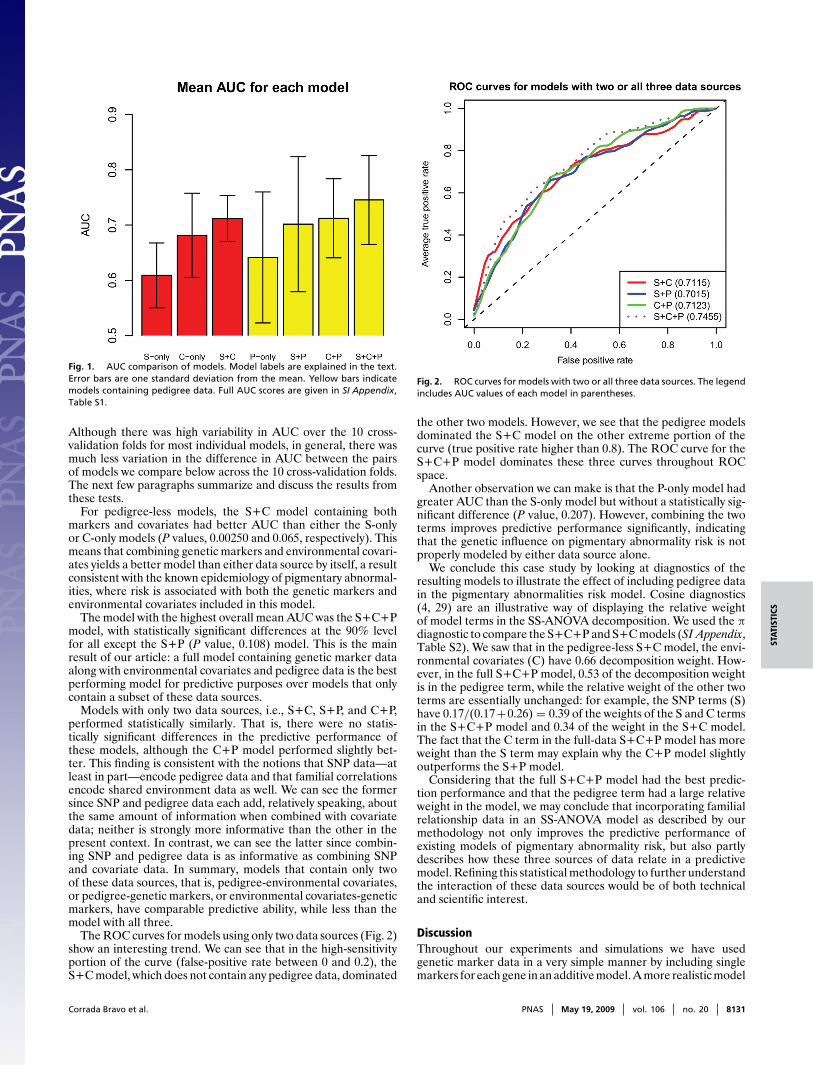
We used area under the receiver operating characteristic (ROC)curve (28, referred to as AUC) estimated by using 10-fold cross-validation to compare predictive performance of models withvarious component combinations. Fig. 1 summarizes our resultsbyplotting the mean AUC of each model. For pedigree models, Fig.1 shows the best AUC of either using RKE to define the pedi-gree kernel or an alternative method described in Materials andMethods. We include full results in SI Appendix. We can observelarge variation in the AUC reported for most model/method com-binations over the cross-validation folds, but some features areapparent: for example, the model with highest overall mean AUCis the S+C+P model. We carried out pairwise t tests on a fewmodel comparisons and report P values from estimates wherevariance is calculated from the differences in AUC between thepair of models being compared over the 10 cross-validation folds.

Table 1. Environmental covariates for BDES pigmentaryabnormality risk SS-ANOVA model

Code Units Description

horm yes/no Current usage of hormone replacement therapyhist yes/no History of heavy drinkingbmi kg/m2 Body mass indexage years Age at baselinesysbp mmHg Systolic blood pressurechol mg/dL Total serum cholesterolsmoke yes/no History of smoking

8130 www.pnas.org / cgi / doi / 10.1073 / pnas.0902906106 Corrada Bravo et al.

STAT

ISTI

CS

Fig. 1. AUC comparison of models. Model labels are explained in the text.Error bars are one standard deviation from the mean. Yellow bars indicatemodels containing pedigree data. Full AUC scores are given in SI Appendix,Table S1.

Although there was high variability in AUC over the 10 cross-validation folds for most individual models, in general, there wasmuch less variation in the difference in AUC between the pairsof models we compare below across the 10 cross-validation folds.The next few paragraphs summarize and discuss the results fromthese tests.

For pedigree-less models, the S+C model containing bothmarkers and covariates had better AUC than either the S-onlyor C-only models (P values, 0.00250 and 0.065, respectively). Thismeans that combining genetic markers and environmental covari-ates yields a better model than either data source by itself, a resultconsistent with the known epidemiology of pigmentary abnormal-ities, where risk is associated with both the genetic markers andenvironmental covariates included in this model.

The model with the highest overall mean AUC was the S+C+Pmodel, with statistically significant differences at the 90% levelfor all except the S+P (P value, 0.108) model. This is the mainresult of our article: a full model containing genetic marker dataalong with environmental covariates and pedigree data is the bestperforming model for predictive purposes over models that onlycontain a subset of these data sources.

Models with only two data sources, i.e., S+C, S+P, and C+P,performed statistically similarly. That is, there were no statis-tically significant differences in the predictive performance ofthese models, although the C+P model performed slightly bet-ter. This finding is consistent with the notions that SNP data—atleast in part—encode pedigree data and that familial correlationsencode shared environment data as well. We can see the formersince SNP and pedigree data each add, relatively speaking, aboutthe same amount of information when combined with covariatedata; neither is strongly more informative than the other in thepresent context. In contrast, we can see the latter since combin-ing SNP and pedigree data is as informative as combining SNPand covariate data. In summary, models that contain only twoof these data sources, that is, pedigree-environmental covariates,or pedigree-genetic markers, or environmental covariates-geneticmarkers, have comparable predictive ability, while less than themodel with all three.

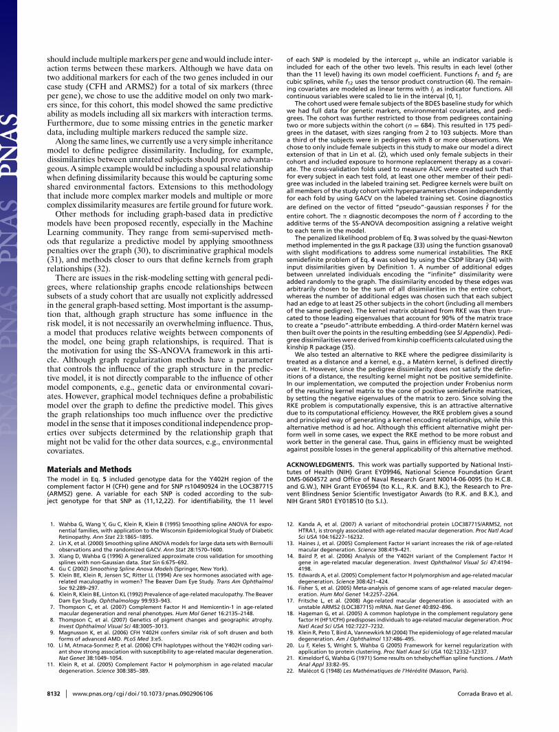
The ROC curves for models using only two data sources (Fig. 2)show an interesting trend. We can see that in the high-sensitivityportion of the curve (false-positive rate between 0 and 0.2), theS+C model, which does not contain any pedigree data, dominated

Fig. 2. ROC curves for models with two or all three data sources. The legendincludes AUC values of each model in parentheses.

the other two models. However, we see that the pedigree modelsdominated the S+C model on the other extreme portion of thecurve (true positive rate higher than 0.8). The ROC curve for theS+C+P model dominates these three curves throughout ROCspace.

Another observation we can make is that the P-only model hadgreater AUC than the S-only model but without a statistically sig-nificant difference (P value, 0.207). However, combining the twoterms improves predictive performance significantly, indicatingthat the genetic influence on pigmentary abnormality risk is notproperly modeled by either data source alone.

We conclude this case study by looking at diagnostics of theresulting models to illustrate the effect of including pedigree datain the pigmentary abnormalities risk model. Cosine diagnostics(4, 29) are an illustrative way of displaying the relative weightof model terms in the SS-ANOVA decomposition. We used the )diagnostic to compare the S+C+P and S+C models (SI Appendix,Table S2). We saw that in the pedigree-less S+C model, the envi-ronmental covariates (C) have 0.66 decomposition weight. How-ever, in the full S+C+P model, 0.53 of the decomposition weightis in the pedigree term, while the relative weight of the other twoterms are essentially unchanged: for example, the SNP terms (S)have 0.17/(0.17+0.26) = 0.39 of the weights of the S and C termsin the S+C+P model and 0.34 of the weight in the S+C model.The fact that the C term in the full-data S+C+P model has moreweight than the S term may explain why the C+P model slightlyoutperforms the S+P model.

Considering that the full S+C+P model had the best predic-tion performance and that the pedigree term had a large relativeweight in the model, we may conclude that incorporating familialrelationship data in an SS-ANOVA model as described by ourmethodology not only improves the predictive performance ofexisting models of pigmentary abnormality risk, but also partlydescribes how these three sources of data relate in a predictivemodel. Refining this statistical methodology to further understandthe interaction of these data sources would be of both technicaland scientific interest.

DiscussionThroughout our experiments and simulations we have usedgenetic marker data in a very simple manner by including singlemarkers for each gene in an additive model. A more realistic model

Corrada Bravo et al. PNAS May 19, 2009 vol. 106 no. 20 8131

should include multiple markers per gene and would include inter-action terms between these markers. Although we have data ontwo additional markers for each of the two genes included in ourcase study (CFH and ARMS2) for a total of six markers (threeper gene), we chose to use the additive model on only two mark-ers since, for this cohort, this model showed the same predictiveability as models including all six markers with interaction terms.Furthermore, due to some missing entries in the genetic markerdata, including multiple markers reduced the sample size.

Along the same lines, we currently use a very simple inheritancemodel to define pedigree dissimilarity. Including, for example,dissimilarities between unrelated subjects should prove advanta-geous. A simple example would be including a spousal relationshipwhen defining dissimilarity because this would be capturing someshared environmental factors. Extensions to this methodologythat include more complex marker models and multiple or morecomplex dissimilarity measures are fertile ground for future work.

Other methods for including graph-based data in predictivemodels have been proposed recently, especially in the MachineLearning community. They range from semi-supervised meth-ods that regularize a predictive model by applying smoothnesspenalties over the graph (30), to discriminative graphical models(31), and methods closer to ours that define kernels from graphrelationships (32).

There are issues in the risk-modeling setting with general pedi-grees, where relationship graphs encode relationships betweensubsets of a study cohort that are usually not explicitly addressedin the general graph-based setting. Most important is the assump-tion that, although graph structure has some influence in therisk model, it is not necessarily an overwhelming influence. Thus,a model that produces relative weights between components ofthe model, one being graph relationships, is required. That isthe motivation for using the SS-ANOVA framework in this arti-cle. Although graph regularization methods have a parameterthat controls the influence of the graph structure in the predic-tive model, it is not directly comparable to the influence of othermodel components, e.g., genetic data or environmental covari-ates. However, graphical model techniques define a probabilisticmodel over the graph to define the predictive model. This givesthe graph relationships too much influence over the predictivemodel in the sense that it imposes conditional independence prop-erties over subjects determined by the relationship graph thatmight not be valid for the other data sources, e.g., environmentalcovariates.

Materials and MethodsThe model in Eq. 5 included genotype data for the Y402H region of thecomplement factor H (CFH) gene and for SNP rs10490924 in the LOC387715(ARMS2) gene. A variable for each SNP is coded according to the sub-ject genotype for that SNP as (11,12,22). For identifiability, the 11 level

of each SNP is modeled by the intercept µ, while an indicator variable isincluded for each of the other two levels. This results in each level (otherthan the 11 level) having its own model coefficient. Functions f1 and f2 arecubic splines, while f12 uses the tensor product construction (4). The remain-ing covariates are modeled as linear terms with Ij as indicator functions. Allcontinuous variables were scaled to lie in the interval [0, 1].

The cohort used were female subjects of the BDES baseline study for whichwe had full data for genetic markers, environmental covariates, and pedi-grees. The cohort was further restricted to those from pedigrees containingtwo or more subjects within the cohort (n = 684). This resulted in 175 pedi-grees in the dataset, with sizes ranging from 2 to 103 subjects. More thana third of the subjects were in pedigrees with 8 or more observations. Wechose to only include female subjects in this study to make our model a directextension of that in Lin et al. (2), which used only female subjects in theircohort and included exposure to hormone replacement therapy as a covari-ate. The cross-validation folds used to measure AUC were created such thatfor every subject in each test fold, at least one other member of their pedi-gree was included in the labeled training set. Pedigree kernels were built onall members of the study cohort with hyperparameters chosen independentlyfor each fold by using GACV on the labeled training set. Cosine diagnosticsare defined on the vector of fitted “pseudo”-gaussian responses f̂ for theentire cohort. The ) diagnostic decomposes the norm of f̂ according to theadditive terms of the SS-ANOVA decomposition assigning a relative weightto each term in the model.

The penalized likelihood problem of Eq. 3 was solved by the quasi-Newtonmethod implemented in the gss R package (33) using the function gssanova0with slight modifications to address some numerical instabilities. The RKEsemidefinite problem of Eq. 4 was solved by using the CSDP library (34) withinput dissimilarities given by Definition 1. A number of additional edgesbetween unrelated individuals encoding the “infinite” dissimilarity wereadded randomly to the graph. The dissimilarity encoded by these edges wasarbitrarily chosen to be the sum of all dissimilarities in the entire cohort,whereas the number of additional edges was chosen such that each subjecthad an edge to at least 25 other subjects in the cohort (including all membersof the same pedigree). The kernel matrix obtained from RKE was then trun-cated to those leading eigenvalues that account for 90% of the matrix traceto create a “pseudo”-attribute embedding. A third-order Matérn kernel wasthen built over the points in the resulting embedding (see SI Appendix). Pedi-gree dissimilarities were derived from kinship coefficients calculated using thekinship R package (35).

We also tested an alternative to RKE where the pedigree dissimilarity istreated as a distance and a kernel, e.g., a Matérn kernel, is defined directlyover it. However, since the pedigree dissimilarity does not satisfy the defin-itions of a distance, the resulting kernel might not be positive semidefinite.In our implementation, we computed the projection under Frobenius normof the resulting kernel matrix to the cone of positive semidefinite matrices,by setting the negative eigenvalues of the matrix to zero. Since solving theRKE problem is computationally expensive, this is an attractive alternativedue to its computational efficiency. However, the RKE problem gives a soundand principled way of generating a kernel encoding relationships, while thisalternative method is ad hoc. Although this efficient alternative might per-form well in some cases, we expect the RKE method to be more robust andwork better in the general case. Thus, gains in efficiency must be weightedagainst possible losses in the general applicability of this alternative method.

ACKNOWLEDGMENTS. This work was partially supported by National Insti-tutes of Health (NIH) Grant EY09946, National Science Foundation GrantDMS-0604572 and Office of Naval Research Grant N0014-06-0095 (to H.C.B.and G.W.), NIH Grant EY06594 (to K.L., R.K. and B.K.), the Research to Pre-vent Blindness Senior Scientific Investigator Awards (to R.K. and B.K.), andNIH Grant 5R01 EY018510 (to S.I.).

1. Wahba G, Wang Y, Gu C, Klein R, Klein B (1995) Smoothing spline ANOVA for expo-nential families, with application to the Wisconsin Epidemiological Study of DiabeticRetinopathy. Ann Stat 23:1865–1895.

2. Lin X, et al. (2000) Smoothing spline ANOVA models for large data sets with Bernoulliobservations and the randomized GACV. Ann Stat 28:1570–1600.

3. Xiang D, Wahba G (1996) A generalized approximate cross validation for smoothingsplines with non-Gaussian data. Stat Sin 6:675–692.

4. Gu C (2002) Smoothing Spline Anova Models (Springer, New York).5. Klein BE, Klein R, Jensen SC, Ritter LL (1994) Are sex hormones associated with age-

related maculopathy in women? The Beaver Dam Eye Study. Trans Am OphthalmolSoc 92:289–297.

6. Klein R, Klein BE, Linton KL (1992) Prevalence of age-related maculopathy. The BeaverDam Eye Study. Ophthalmology 99:933–943.

7. Thompson C, et al. (2007) Complement Factor H and Hemicentin-1 in age-relatedmacular degeneration and renal phenotypes. Hum Mol Genet 16:2135–2148.

8. Thompson C, et al. (2007) Genetics of pigment changes and geographic atrophy.Invest Ophthalmol Visual Sci 48:3005–3013.

9. Magnusson K, et al. (2006) CFH Y402H confers similar risk of soft drusen and bothforms of advanced AMD. PLoS Med 3:e5.

10. Li M, Atmaca-Sonmez P, et al. (2006) CFH haplotypes without the Y402H coding vari-ant show strong association with susceptibility to age-related macular degeneration.Nat Genet 38:1049–1054.

11. Klein R, et al. (2005) Complement Factor H polymorphism in age-related maculardegeneration. Science 308:385–389.

12. Kanda A, et al. (2007) A variant of mitochondrial protein LOC387715/ARMS2, notHTRA1, is strongly associated with age-related macular degeneration. Proc Natl AcadSci USA 104:16227–16232.

13. Haines J, et al. (2005) Complement Factor H variant increases the risk of age-relatedmacular degeneration. Science 308:419–421.

14. Baird P, et al. (2006) Analysis of the Y402H variant of the Complement Factor Hgene in age-related macular degeneration. Invest Ophthalmol Visual Sci 47:4194–4198.

15. Edwards A, et al. (2005) Complement factor H polymorphism and age-related maculardegeneration. Science 308:421–424.

16. Fisher S, et al. (2005) Meta-analysis of genome scans of age-related macular degen-eration. Hum Mol Genet 14:2257–2264.

17. Fritsche L, et al. (2008) Age-related macular degeneration is associated with anunstable ARMS2 (LOC387715) mRNA. Nat Genet 40:892–896.

18. Hageman G, et al. (2005) A common haplotype in the complement regulatory genefactor H (HF1/CFH) predisposes individuals to age-related macular degeneration. ProcNatl Acad Sci USA 102:7227–7232.

19. Klein R, Peto T, Bird A, Vannewkirk M (2004) The epidemiology of age-related maculardegeneration. Am J Ophthalmol 137:486–495.

20. Lu F, Keles S, Wright S, Wahba G (2005) Framework for kernel regularization withapplication to protein clustering. Proc Natl Acad Sci USA 102:12332–12337.

21. Kimeldorf G, Wahba G (1971) Some results on tchebycheffian spline functions. J MathAnal Appl 33:82–95.

22. Malécot G (1948) Les Mathématiques de l’Hérédité (Masson, Paris).

8132 www.pnas.org / cgi / doi / 10.1073 / pnas.0902906106 Corrada Bravo et al.

STAT

ISTI

CS

23. Klein R, Klein B, Linton K, De Mets D (1991) The Beaver Dam Eye Study: Visual acuity.Ophthalmology 98:1310–1315.

24. Klein R, et al. (2007) Fifteen-year cumulative incidence of age-related maculardegeneration: The Beaver Dam Eye Study. Ophthalmology 114:253–262.

25. Klein R, Klein B, Tomany S, Meuer S, Huang G (2002) Ten-year incidence and pro-gression of age-related maculopathy: The Beaver Dam eye study. Ophthalmology109:1767–1779.

26. Klein R, Klein B, Jensen S, Meuer S (1997) The five-year incidence and progression ofage-related maculopathy: The Beaver Dam Eye Study. Ophthalmology 104:7–21.

27. Lee K, Klein B, Klein R, Knudtson M (2004) Familial aggregation of retinal vessel caliberin the Beaver Dam Eye Study. Invest Ophthalmol Visual Sci 45:3929–3933.

28. Fawcett T (2006) An introduction to roc analysis. Pattern Recognit Lett 27:861–874.29. Gu C (1992) Diagnostics for nonparametric regression models with additive terms.

J Am Stat Assoc 87:1051–1058.

30. Sindhwani V, Niyogi P, Belkin M (2005) Beyond the point cloud: From transductive tosemi-supervised learning. ACM Int Conf Proc Ser 119:824–831.

31. Chu W, Sindhwani V, Ghahramani Z, Keerthi S (2007) Relational learning with gauss-ian processes. Advances in Neural Information Processing Systems: Proceedings of the2006 Conference (MIT Press, Cambridge, MA).

32. Smola A, Kondor R (2003) Kernels and regularization on graphs. Conference onLearning Theory (Springer Verlag, Heidelberg, Germany), pp. 144–158.

33. Gu C (2007) gss: General smoothing splines. R package version 1.0-0. Available at:http://cran.r-project.org/web/packages/gss/index.html. Accessed February 13, 2008.

34. Borchers B (1999) CSDP: A C library for semidefinite programming. Optimiz MethodsSoftware 11:613–623.

35. Atkinson B, Therneau T (2007) Kinship: Mixed-Effects Cox Models, Sparse Matrices,and Modeling Data from Large Pedigrees. R package version 1.1.0-18. Available at:http://cran.r-project.org/web/packages/kinship/index.html. Accessed June 22, 2008.

Corrada Bravo et al. PNAS May 19, 2009 vol. 106 no. 20 8133