Examining the relationship between the exchange rate

Louisiana State UniversityLSU Digital Commons

LSU Doctoral Dissertations Graduate School

2012

Examining the relationship between the exchangerate, foreign direct investment and tradeShanta ParajuliLouisiana State University and Agricultural and Mechanical College

Follow this and additional works at: https://digitalcommons.lsu.edu/gradschool_dissertations

Part of the Agricultural Economics Commons

This Dissertation is brought to you for free and open access by the Graduate School at LSU Digital Commons. It has been accepted for inclusion inLSU Doctoral Dissertations by an authorized graduate school editor of LSU Digital Commons. For more information, please [email protected].

Recommended CitationParajuli, Shanta, "Examining the relationship between the exchange rate, foreign direct investment and trade" (2012). LSU DoctoralDissertations. 2670.https://digitalcommons.lsu.edu/gradschool_dissertations/2670

https://digitalcommons.lsu.edu?utm_source=digitalcommons.lsu.edu%2Fgradschool_dissertations%2F2670&utm_medium=PDF&utm_campaign=PDFCoverPages

https://digitalcommons.lsu.edu/gradschool_dissertations?utm_source=digitalcommons.lsu.edu%2Fgradschool_dissertations%2F2670&utm_medium=PDF&utm_campaign=PDFCoverPages

https://digitalcommons.lsu.edu/gradschool?utm_source=digitalcommons.lsu.edu%2Fgradschool_dissertations%2F2670&utm_medium=PDF&utm_campaign=PDFCoverPages

https://digitalcommons.lsu.edu/gradschool_dissertations?utm_source=digitalcommons.lsu.edu%2Fgradschool_dissertations%2F2670&utm_medium=PDF&utm_campaign=PDFCoverPages

http://network.bepress.com/hgg/discipline/1225?utm_source=digitalcommons.lsu.edu%2Fgradschool_dissertations%2F2670&utm_medium=PDF&utm_campaign=PDFCoverPages

https://digitalcommons.lsu.edu/gradschool_dissertations/2670?utm_source=digitalcommons.lsu.edu%2Fgradschool_dissertations%2F2670&utm_medium=PDF&utm_campaign=PDFCoverPages

mailto:[email protected]

EXAMINING THE RELATIONSHIP BETWEEN THE EXCHANGE RATE,

FOREIGN DIRECT INVESTMENT AND TRADE

A Dissertation

Submitted to the Graduate Faculty Louisiana State University and

Agricultural and Mechanical College in partial fulfillment of the

requirement for the degree of Doctor of Philosophy

in Department of Agricultural Economics and Agribusiness

By Shanta Parajuli

B.S., Prithivi Narayan Campus, Tribhuvan University, Nepal, 1997 M.Sc., Tribhuvan University, Nepal, 2000

M.S., Alabama Agricultural and Mechanical University, 2006 May, 2012

ii

Dedication

I dedicate this dissertation to the almighty God for giving me the strength and courage to continue. To my parents for giving me strength.

iii

Acknowledgements

This dissertation was made possible with the guidance, support, and inspiration of many people,

but most importantly, my committee members, friends and family. First and foremost, I would

like to express my deepest gratitude and sincere thanks to my honorable advisor, Dr. P. Lynn

Kennedy, for his guidance, wisdom and friendship. It has been a great honor and an

extraordinary learning experience to work under his direction.

I would also like to express my deepest appreciations to the distinguished members of

my dissertation committee Dr. Michael E. Salassi, Dr. R. Wes Harrison, and Dr. John Westra.

Their support provided me with direction and a vision to complete this dissertation.

I would like to thank Dr. Hongyu He from the Department of Mathematics as the dean

representative for my dissertation. I would also like to acknowledge Brain Hilbun for careful

editing.

I thank Dr. Gail L. Cramer, the head of the Agricultural Economics and Agribusiness

Department, for providing me with financial support throughout the study. Your every word is

always encouraging. Again thank you very much.

Thanks for my all friends, classmates and officemates who made my stay at the

University memorable and valuable. I would like to thank Pablo Garcia for his guidance on data

source information and providing me with articles on FDI at the beginning of the research.

My deepest gratitude goes to my brother-in-laws, sister-in-laws, father-in-law and

mother-in-law for their unweaving support and encouragement throughout my graduate

milestone. Without their support, I would not have been able to achieve my goal.

iv

I would like to thanks for my parents for their endless love and encouragement

throughout my study. Last but not least, my deepest gratuities go to my husband Pradip Adhilari

for his love and patient. To my son Ankit Adhikari for his endless patient and understanding me

thorough this long journey

v

Table of Contents

Dedication ................................................................................................................................. ii Acknowledgements .................................................................................................................. iii List of Tables .......................................................................................................................... vii List of Figures ........................................................................................................................ viii Abstract .................................................................................................................................... ix Chapter 1: Introduction ............................................................................................................. 1 1.1 Introduction ......................................................................................................................... 1 1.1 Problem Statement of the Study ......................................................................................... 2 1.2 Research Objectives ............................................................................................................ 3 1.3 Justification of the Study .................................................................................................... 3 1.4 Outline of the Dissertation .................................................................................................. 4 1.5 References ........................................................................................................................... 5 Chapter 2: The Exchange Rate and Inward Foreign Direct Investment in Mexico .................. 9 2.1 Introduction ......................................................................................................................... 9 2.2. Literature Review............................................................................................................. 14 2.2.1 Determinant of Foreign Direct Investment ................................................................. 14 2.2.2 Foreign Direct Investment and Exchange Rate .......................................................... 17 2.3 Methodology and Data ...................................................................................................... 20 2.3.1 The Model ................................................................................................................... 20 2.3.2 Data ............................................................................................................................. 26 2.3.3 Econometric Estimation .............................................................................................. 27 2.4 Result and Discussion ....................................................................................................... 30 2.5 Conclusion ........................................................................................................................ 36 2.6 References ......................................................................................................................... 39 Chapter 3: U.S. Foreign Direct Investment and U.S. Exports to Mexico: The Case of the Processed Food and Manufacturing Sectors and NAFTA ...................................................... 47 3.1 Introduction ....................................................................................................................... 47 3.2 Literature Review.............................................................................................................. 50 3.2.1 Total FDI ..................................................................................................................... 50 3.2.2 FDI in Processed Food and Manufacturing Sectors ................................................... 52 3.3 Methodology and Data ...................................................................................................... 55 3.3.1 The Model ................................................................................................................... 55 3.3.2 Data ............................................................................................................................. 59 3.3.3 Econometric Estimation .............................................................................................. 62 3.3.3.1 Unit Root Tests .................................................................................................. 62 3.3.3.2 ARDL Bounds Testing Approach ...................................................................... 63 3.4 Result and Discussion ....................................................................................................... 68 3.4.1 Unit Roots Test ........................................................................................................... 68

vi

3.4.2 ARDL Bounds Test Results ........................................................................................ 71 3.5 Conclusion ........................................................................................................................ 80 3.6 References ......................................................................................................................... 82 Chapter 4: Relationship among Foreign Direct Investment, Economic Growth and Exports in Mexico .................................................................................................................................... 89 4.1 Introduction ....................................................................................................................... 89 4.1.1 Economic Growth in Mexico ...................................................................................... 91 4.2 Literature Review.............................................................................................................. 94 4.2.1 Granger Causality Studies on Panel Data ................................................................... 94 4.2.2 Granger Causality Studies on Individual Countries .................................................... 95 4.2.3 Granger Causality Studies in Mexico ......................................................................... 97 4.3 Methodology and Data ...................................................................................................... 98 4.3.1 The Model ................................................................................................................... 98 4.3.2 Data ........................................................................................................................... 101 4.4.3 Econometric Methods ............................................................................................... 101 4.4 Result and Discussion ..................................................................................................... 105 4.4.1. Unit root test ............................................................................................................ 105 4.4.2 The VAR Model and Granger Causality Test........................................................... 106 4.5 Conclusions ..................................................................................................................... 114 4.6 References ....................................................................................................................... 117 Chapter 5: Summary and Conclusion ................................................................................... 124 5.1 References ....................................................................................................................... 128 Appendix 2.1 Inflows and outflows of foreign direct investment (U.S. $ Billions) ............. 129 Appendix 2.2 Variable definitions and data sources ............................................................ 130 Appendix 3.1 Plots of the Variables ..................................................................................... 131 Appendix 3.2 Summary of statistics of U.S. affiliates sales to local market (Mexico), United States and others countries .................................................................................................... 138 Appendix 3.3 Variables definitions and source of data ........................................................ 139 Appendix 3.4 Summary of statistics of the variables ........................................................... 140 Appendix 4.1 Variable descriptions and source of data ....................................................... 141 Appendix 4.2 Summary Statistics of the Variables .............................................................. 142 Appendix 4.3 List of the variables that are in each model .................................................... 143 Vita ........................................................................................................................................ 144

vii

List of Tables

Table 2.1 FDI inflows in millions of dollars to Mexico, 1985 to 2009 ........................................ 11

Table 2.2 Results of the Poisson regression.................................................................................. 32

Table 3.1 ADF and PP unit root tests ........................................................................................... 69

Table 3.2 Zivot and Andrews and Perron and Vogelsang tests for unit roots .............................. 70

Table 3.3 Diagnostic tests for the ARDL equation ....................................................................... 72

Table 3.4 Results from bounds tests on equations 3.10 for the existence of a long-run relationship……………………………………………………………………………………….73

Table 3.5 Estimated long- run coefficients using the ARDL (2,2,2,0,0,2) approach .................. 75

Table 3.6 Error correction representation for the selected ARDL (2,2,2,0,0,2) model ................ 79

Table 3.7 Diagnostic tests for the error correction for the ARDL (2,2,2,0,0,2) model ................ 80

Table 4. 1Tests of the unit root hypothesis with trend and constant and constant only ............. 107

Table 4.2 Misspecification tests for augmented VAR (2) .......................................................... 108

Table 4. 3 Misspecification tests for estimated endogenous equations ...................................... 109

Table 4.4 Granger causality results using MWALD test (TYDL method) for Model 1 and 2 ... 110

Table 4.5 Granger causality results using MWALD test (TYDL method) for Model 3, 4 and 5111

Table 4.6 Granger causality results using MWALD test (TYDL method) for Model 6 ............ 113

viii

List of Figures

Figure 2.1 Foreign direct investment inflows and outflows in OECD countries .......................... 10

Figure 2.2 Foreign direct investment inflows allocation in Mexico ............................................. 13

Figure 3.1 Total sales (TFDI), manufacturing sales (MFDI) and processed food sales (FFDI) as percent of Mexico GDP by U.S. affiliates in Mexico ................................................................... 60

Figure 3.2 U.S. total exports (TEXP), manufacturing export (MEXP), and processed food export

(FEXP) as percent of Mexico GDP .............................................................................................. 61

Figure 4.1 GDP and Exports growth rates (percent), 1960 to 2009 ............................................. 92

Figure 4.2 FDI inflows into Mexico (percent of GDP), 1970 to 2009 ......................................... 93

ix

Abstract

Extensive research has been carried out on the relationships among foreign direct investment

(FDI), exports, the exchange rate, and economic growth. However, these research findings are

mixed and inconclusive. Therefore, further research and discussion are needed on this topic.

This study focused on Mexico, since it is one of the major FDI recipient countries in Latin

America and much of its trade is a result of its free trade agreements. This study examines the

relationship between FDI, exports, and economic growth in the context of FDI from developed to

developing countries (Mexico).

The second chapter analyzes the relationship of FDI with the level of the exchange rate,

exchange rate volatility, and exchange rate expectations during the period from 1994 to 2008.

The analysis revealed a significant impact of level of exchange rates and exchange rate

expectations on FDI flows. Regional trade agreements, such as the European Union (EU) and

the North American Free Trade Agreement (NAFTA), were important factors to attract FDI.

The third chapter examines the long-run relationship between U.S. FDI and U.S exports

to Mexico from 1988Q1 to 2008Q4. This analysis found a complementary (positive) relationship

between FDI and exports. However, the strength of the relationship differs with different types of

FDI. The analysis further revealed a weak complementary relationship with exports of processed

food and a strong positive relationship with manufacturing exports. The study also showed a

significant impact of NAFTA on manufacturing and total FDI and an insignificant impact on

processed food FDI.

Chapter four examined Granger causality among GDP, exports, and FDI in Mexico for

the period of 1970 to 2008. The causality was tested from the bivariate to the multivariate

x

framework using Toda and Yamamoto (1995) and Doland and Lutkepohl (1996) (TYDL)

methodologies. An important finding in this study is the Ganger causality from gross fixed

capital formation and labor force to imports. The results suggest that the Granger causality

between GDP and exports; FDI and GDP; exports and FDI observed in two, three or four

variable frameworks are through a channel of imports.

1

Chapter 1: Introduction

1.1 Introduction

Over the last three decades, Foreign Direct Investment (FDI) has emerged as one of the most

important sources of globalization and an important catalyst for economic growth, transferring

technology and knowledge between participating countries. FDI also provides opportunities and

financial challenges around the world. There exists extensive literature related to FDI inflows

and outflows (Barrell and Pain, 1996; Blonigen, 1997; Coughlin, et al., 1991; Cushman, 1988;

Pain, 1993). The theories related to the types of FDI suggest two types of FDI: horizontal

(market-seeking) and vertical. The international market searching for the lowest cost of

production is called vertical FDI, which is mainly export oriented (Shatz and Venables, 2000).

Horizontal FDI refers to the establishment of homogenous plants in foreign locations as a means

of supplying certain goods in a foreign country. This type of FDI replaces exports from the home

country to the host country.

The exchange rate is a crucial factor of FDI flows and some studies on FDI determinants

have integrated the exchange rate (Amuedo-Dorantes and Pozo, 2001; Barrel and Pain, 1998;

Blonigen, 1997; Buch and Kleinert, 2008; Campa, 1993; Crowley and Lee, 2003; Goldberg and

Kolstad, 1995; Guo and Trividi 2002; 1994; Schmidt and Broll, 2009; Steveen 1998; Russ, 2007;

Waldkirch, 2003). Previous studies (Barrel and Pain 1998; Klein and Rosengren, 1994; Guo and

Trividi, 2002; Buch and Kleinert, 2008) suggest that a depreciation of the host country’s

currency attracts FDI. In the meantime, other research (Waldkirch, 2003; Campa; Schmidt and

Broll, 2009; Amuedo-Dorantes and Pozo, 2001) argues that the appreciation of the host currency

attracts FDI.

2

Mexico is one of the most open market countries in the world (Villarreal, 2010). It joined

the OECD in 1994 and is one of the few developing members of the OECD. In the same year,

Mexico, the United States and Canada implemented the North American Free Trade Agreement

(NAFTA) to reduce trade barriers among Canada, the United States, and Mexico and encourage

FDI among the three countries. Previously, under the General Agreement on Tariffs and Trade

(GATT), Mexico imposed tariffs of 90%-100% on imported goods and often required import

licenses. After NAFTA, the Mexican tariff rates were reduced dramatically, averaging 20% and

the requirement for import licensing was largely eliminated (Qasmi and Fausti, 2001).

1.1 Problem Statement of the Study

Trade and FDI are two channels where the firm gains access to the intended market.

Fluctuations of the exchange rate generate complications in the international market and affect

economies. Appreciation of the home currency may have positive or negative impacts on

trade/FDI. The relationship between the exchange rate and FDI has long been discussed in

literature, but there still exists controversy on the direction in which the effect will occur.

Complementary and substitutionary relationships between FDI and exports are both

reported in previous literature (Alguacila and Ortsa, 2003; Bajo-Rubio and Montero-Munoz,

2001; Head and Ries, 2001; Marchant et al., 2002; Ning and Reed, 1995; Pfaffermayer, 1996),

but the literature on the relationship between processed food and manufacturing FDI with

exports is sparse. Some literature has reported a complementary relationship (Bolling and

Somwaru, 2001; Kim and Kang, 1996; Marchant et al., 2002), while most of studies focused on

developing countries where raw inputs are imported by foreign affiliates in the host country.

Others studies revealed substitutionary relationships (Blonigen, 1997; Malanoski et al., 1997),

3

therefore the issue has still not been resolved. The strength of the relationship may also be weak

or strong depending on the exchange rate. Furthermore, regional trade agreements and exports-

oriented policies of countries have treated exports as the principal channel through which

openness can promote economic growth (Export-led growth). In addition to this, a stronger

impact of FDI on economic growth is found for export oriented policies than for import oriented

policies. Results are mixed with respect to FDI-led growth as well as export-led growth. The

results differ according to the country examined, time of study, and econometric method used.

The majority of studies testing these relationships were conducted based on a two variable

context. This study will test the direction of causality using five variables.

1.2 Research Objectives

The overall objective of this study was to test the effect of the exchange rate on FDI and the

effect of FDI and exports on economic growth in Mexico. Specific objectives of this study are:

1) To determine the relationship between the exchange rate and FDI inflows into Mexico

from OECD countries;

2) To determine the long- run relationship between FDI and exports in Mexican processed

food and manufacturing industry types of FDI; and,

3) To test the direction of causality among FDI, exports, and growth in Mexico.

1.3 Justification of the Study

Mexico is the largest FDI recipient in Latin America (UNCTAD, 2002) and among developing

countries, the second largest trading country in terms of trade (WTO, 2001). One of the main

4

factors is Mexico’s location. Mexico offers its services to the entire North American market,

rather than just its domestic market (Graham and Wada, 2000). The successful increase in trade

has been accompanied by United States foreign direct investment (FDI) in Mexico following the

implementation of NAFTA.

Mexican trade policies of 1980 and NAFTA effectively linked the Mexican economy

with the global economy and that of the United States. The growth rate of real gross domestic

product (GDP) averaged 2.29% per year during 1981-2009. The growth rate after NAFTA and

the peso crisis (1996-2009) averaged 2.84%. This growth rate is lower compared to the import

substitution trade policy of Mexico. Therefore, this analysis will determine the effect of the

exchange rate on FDI inflows into Mexico as well as the direction of causalities among FDI,

exports, and growth. This will shed light on the inflows of FDI to a developing country from

developed countries, the relationship between FDI and exports and the direction of causalities

among FDI, exports, and growth.

1.4 Outline of the Dissertation

This dissertation is formatted in three “journal-article style” chapters. The second chapter

analyzes the relationship between FDI and the exchange rate, exchange rate volatility, and

exchange rate expectations. This analysis uses FDI outflows from OECD countries to Mexico

using data from 1994 to 2008. All variables are measured on the 2005 price basis (in U.S.

dollars). The PPML method (Santos and Tenreyo, 2006) was used to estimate the gravity model.

The third chapter determines the long-run relationship between FDI and exports. This

relationship is examined under three different types of FDI (processed food, manufacturing, and

5

total). This analysis utilized quarterly data from 1988Q1 to 2008Q4. The autoregressive

distributed lag model (ARDL) developed by Pesaran et al. (2001) was used to test the

relationship. The impact of NAFTA on the relationship between FDI and exports was also

determined.

Chapter four tested the direction of casualties among FDI, exports, and growth in

Mexico. This analysis uses data from 1980 to 2008. The modified Wald statistic was used to test

the causal relationship. Model 1 and 3 were in the bivariate framework. In Model 2 and 5,

imports are integrated. Finally, the sixth model is derived from the new growth theory as

employed by Sala-i-Martin (1995) and Fosu (2006) where exports and imports are used as an

additional variable along with labor and capital. Finally, chapter five summarizes the research

findings, discusses policy implications, and considers potential opportunities for future research.

1.5 References

Alguacil, M. T. and Orts, V. (2002). A multivariate cointegrated model testing for temporal causality between exports and outward FDI: The Spanish Case. Applied Economics 34(1): 119-132.

Amuedo-Dorantes, C. and Pozo, S. (2001). Exchange-Rate Uncertainty and Economic

Performance. Review of Development Economics 5 (3): 355-446. Bajo-Rubio, O. and Montero-Muño, M. (2001). Foreign Direct Investment and Trade: A

Causality Analysis. Open Economies Review 12(3): 305-323. Barrell, R. and Pain, N. ( 1998 ). Real exchange rate, agglomerations, and irreversibilities:

macroeconomic policy and FDI in EMU. Oxford Review of Economic Policy 14(3): 152-167.

Barrell, R. and Pain, N. (1996). An Econometric Analysis of U.S. Foreign Direct Investment.

The Review of Economics and Statistics 78(2): 200-207. Barro, R. J. and Sala-i-Martin, X. I. (1995). Economic Growth. McGraw-Hill College.

6

Blonigen, B. A. and Feenstra, R. C. (1997).Protectionist Threats and Foreign Direct Investment. In The Effects of U.S. Trade Protection and Promotion Policies(Ed R. C. Feenstra). University of Chicago Press.

Blonigen, B. A. (1997). Firm-Specific Assets and the Link between Exchange Rates and Foreign

Direct Investment. American Economic Review 87 (3): 447-465. Blonigen, B. A. (2005). A Review of the Empirical Literature on FDI Determinants. Atlantic

Economic Journal Vol. 33 Issue 4, p383(4): 383-403. Bolling, C. and Somwaru, A. (2001). U.S. food companies access foreign markets through direct

investment. Food Review 24(3): 23-28. Buch, C. M. and Kleinert, J. (2008). Exchange Rates and FDI: Goods versus Capital Market

Frictions. The World Economy 31(9): 1185-1207. Campa, J. M. (1993). Entry by foreign firms in the United States under exchange rate

uncertainty. 75 75(4): 614-622. Coughlin, C. C., Terza, J. V. and Arromdee, V. (1991). State Characteristics and the Location of

Foreign Direct Investment within the United States. The Review of Economics and

Statistics 73(4): 675-683 Crowley, P. and Le, J. (2003). Exchange rate volatility and foreign investmetn: international

evidence. The International Trade Journal 17(3): 227-252. Cushman, D. O. (1988). Exchange-rate uncertainty and foreign direct investment in the United

States. Review of World Economy 124(2): 322-336. Fosu, O.-A. E. and Magnus, F. J. (2006). Bounds testing approach to cointegration: an

examination of foreign direct investment trade and growth relations. American Journal of

Applied Sciences 3(11): 2079-2085. Goldberg, L. S. and Kolstad, C. D. (1995). Foreign Direct Investment, Exchange Rate Variability

and Demand Uncertainty. International Economic Review 36(4): 855-873. Guo, J. Q. and Trivedi, P. K. (2002). Firm–Specific Assets and the Link between Exchange

Rates and Japanese Foreign Direct Investment in the United States: A Re–examination. Japanese Economic Review 53(3): 337-349.

Head, K. and Ries, J. (2008). FDI as an outcome of the market for corporate control: Theory and

evidence. Journal of International Economics 74 (1): 2-20. Kim, J.-D. and Rang, I.-S. (1997). Outward FDI and exports: The case of South Korea and

Japan. Journal of Asian Economics 8 (1): 39-50.

7

Klein, M. W. and Rosengren, E. (1994). The real exchange rate and foreign direct investment in the United States: Relative wealth vs. relative wage effects. Journal of International Economics 36(3-4): 373-389.

Malanoski, M., Handy, C. and Henderson, D. (1997).Time Dependent Relationship in U.S.

Processed Food Trade and Foreign Direct Investment. In Organization and Performance

of World Food Systems, Vol. 182(Ed S. R. Henneberry). Oklahoma State University. Marchant, M. A., N.Cornell, D. and Koo, W. (2002). International trade and foreign direct :

substitute or complement. Journal of Agricultural and Applied Economics 34(2): 289-302.

Ning, Y. and Reed, M. R. (1995). Locational determinants of the US direct foreign investmetn in

food and kindred products. Agribusiness 11(1): 77-85. Pesaran, M. H., Shin, Y. and Smith, R. J. (2001). Bonds testing approaches to the analysis of

level relationship. Journal of Applied Econometric 16(3): 289- 326. Pfaffermayr, M. (1996). Foreign outward direct investment and exports in Austrian

manufacturing: Substitutes or complements? Review of World Economics 132(3): 501-522.

Qasmi, B. A. and Fausti, S. W. (2001). NAFTA intra-industry trade in agricultural food products.

Agricultural Economics and Resource Management 17(2): 255-271. Russ, K. N. (2007 ). The endogeneity of the exchange rate as a determinant of FDI: A model of

entry and multinational firms. Journal of International Economics 71: 344-372. Schmidt, C. W. and Broll, U. (2009). Real exchange-rate uncertainty and US foreign direct

investment: an empirical analysis. Review of World Economics 145(3): 513-530. Shatz, H. J. and Venables, A. J. (2000).The geography of international investment. In Policy

Research Working Paper SeriesWashington, DC World Bank. Silva, J. M. C. S. and Tenreyro, S. (2006). The log of gravity. The Review of Economics and

Statistics 88(4): 641-658. Stevens, G. V. G. (1998). Exchange Rates and Foreign Direct Investment: A Note. Journal of

Policy Modeling 20 (3): 393-401. UNCTAD (2002).World Investment Report 2002: Transnational Corporations and Export

Competitiveness. New Yrok: United Nation. Villarreal, M. A. (2010).NAFTA and the Mexican Economy. Congressional Research Service.

8

Waldkirch, A. (2003). The 'new regionalism' and foreign direct investment: the case of Mexico. Journal of International Trade and Economic Development 12(2): 151-184.

WTO (2001).International trade statisics 2001.

9

Chapter 2: The Exchange Rate and Inward Foreign Direct Investment in

Mexico

2.1 Introduction

An important part of globalization is the increase in trade as well as foreign direct investment

(FDI), which has occurred around the world. The largest amount of FDI outflows around the

world are from the Organization for Economic Cooperation and Development (OECD) countries.

In 2009, 81% of global outward FDI is reported from OECD countries. In the same year, 57% of

global inflows of FDI were reported for OECD countries. The highest amount of FDI outflows

and inflows is reported in the year 2007 (Figure 2.1 and Appendix 2.1).

For many developing countries, FDI has become an increasingly important source of

external financing (UNCTAD, 2011). It brings recent technology, knowledge, employment as

well as economic growth to a country. Mexico is one of the developing countries among the

member of OECD countries and the largest FDI recipient in Latin America (UNCTAD, 2002).

One of Mexico’s most important trading partners is the United States and most of its (Mexico’s)

exports are targeted to the U.S. market. Therefore, it is no surprise that the economies of both

Mexico and the United States are deeply intertwined. To make Mexico less dependent on the

U.S. economy and to gain some economic benefits, the Mexican government has signed different

trade agreements with various countries (Villarreal, 2010). In 1986, Mexico joined the General

Agreement on Tariffs and Trade (GATT). Before GATT, Mexico imposed tariffs of up to 100%

on imported goods and also required importers to have proper licenses (Qasmi and Fausti, 2001).

Since 1990, Mexico has been one of the most open countries in the world with respect to trade

10

(Villarreal, 2010). It joined both the OECD and North America Free Trade Agreement

(NAFTA) in 1994.

Figure 2.1 Foreign direct investment inflows and outflows in OECD countries Source: Organization for Economic Cooperation and Development (OECD) Statistics online version.

World FDI inflow into Mexico was around U.S. $27 billion in 2007, decreasing to U.S. $14.4

billion in 2009. From OECD member countries, there was approximately U.S. $25 billion of

FDI inflow to Mexico in 2007. This later decreased to U.S. $14 billion in 2009 (Table 2.1). In

2004, approximately U.S. $134 billion of total FDI was allocated to the manufacturing sector

with U.S. $3 billion allocated to food industries (Figure 2.2). Total FDI inflows to Mexico

decreased to U.S. $8 billion in 1995. Thereafter, FDI flows to Mexico have gradually increased.

Furthermore, with Mexico having become a relatively open country (in terms of ease of trading

0500

1,000

1,500

2,000

Billions of dollars

1990

1991

1992

1993

1994

1995

1996

1997

1998

1999

2000

2001

2002

2003

2004

2005

2006

2007

2008

2009

2010

OECD inflows OECD outflowsYear

11

restrictions), its export volume has also increased. Both exports and FDI are also affected by

variations in the exchange rate. Under such a scenario, it is very important to study and analyze

the impacts that exchange rates and fluctuations in exchange rates have on FDI flows.

Table 2.1 FDI inflows in millions of dollars to Mexico, 1985 to 2009

Year W OECD SA EU15 NAFTA EUROPE

1985 5754 3252 -1 777 2040 895 1986 7341 4193 2 1198 2687 1293 1987 5345 2645 -1 678 1373 862 1988 4838 2509 0 616 1838 740 1989 6848 3690 9 928 2397 910 1990 5758 3286 98 825 1941 924 1991 10039 5004 384 1358 3238 1370 1992 14654 7582 66 1475 5826 1523 1993 11229 6260 360 990 4916 987 1994 22827 11326 1048 1951 8124 1898 1995 16822 8139 144 2222 5704 2232 1996 18519 7111 .. 1121 5679 1280 1997 24526 11122 .. 3089 7461 3155 1998 21251 7290 .. 1940 5178 1981 1999 13716 13318 55 3861 8045 3987 2000 17814 17185 102 3189 13389 3343 2001 27168 26331 46 4180 22082 4010 2002 19310 18545 64 4886 12929 5362 2003 15268 14956 49 4638 9810 4980 2004 23673 23297 131 .. 9137 13733 2005 21856 18726 737 .. 12003 6482 2006 19195 18592 115 .. 12886 7062 2007 27174 25196 89 .. 12206 12443 2008 22517 20699 156 .. 11674 8424 2009 14462 14090 189 .. 7855 5846 Total 397905 294343 3839 39922 190418 95723 Total/W 1 0.74 0.02 10.40 4.77 0.50

Source: Organization for Economic Cooperation and Development (OECD) Statistics online version. Own calculation W: World, North American Free Trade Agreement (NAFTA) and South Asia (SA)

Fluctuations in exchange rates and exchange rate volatility in developed countries impact the

economy and generate complications in the international market. The influence that exchange

rates and exchange rate volatility have on FDI has been discussed previously in the literature.

12

However, there is still controversy over the direction in which the effect occurs. The depreciation

of a host currency with respect to the home currency may have either a positive or a negative

effect on FDI flows. Some researchers, such as Campa (1993); Rivoli, (1996), explain the

positive relationship (home per host currency) and others, like Cushman (1985, 1988); Goldber

and Kolstad (1995), suggest a negative relationship. Cushman (1985) included real exchange rate

risk and expectations in their FDI model and concluded that an increase in future changes in the

exchange rate reduce exports, but also attract market- seeking FDI. The negative impact of the

exchange rate on export oriented FDI was reported by Lecraw (1991). In the meantime, Campa

(1993) included expectations of the exchange rate and exchange rate volatility in the model,

suggesting that the depreciation of the host country’s currencies against that of the home

country’s decreases FDI due to the association of the lower level of exchange rate (with the

lower level of expected profit in terms of the home currency). Froot and Stein (1991) established

the capital imperfection theory of exchange rate and suggested that the depreciation of the host

currency is positively related with FDI. The depreciation of the host currencies relatively

increases the wealth of the investors and increases the FDI inflow.

Most of the literature related to FDI inflows/outflows along with exchange rate related

variables have primarily focused on developed rather than less-developed countries. The limited

research on FDI flows into developing countries is attributed to the lack of reliable FDI data, as

well as the shortage of capital in developing countries (Thomas and Grosse, 2001; Majeed and

Ahmad, 2007). FDI inflows into developing countries are mainly due to countries with relatively

low production costs for things such as raw materials and labor (Shatz and Venables, 2000). The

limited amount of research conducted on FDI flows into developing countries motivated me to

study inward FDI into Mexico from developed countries (OECD).

13

Figure 2.2 Foreign direct investment inflows allocation in Mexico Source: Organization for Economic Cooperation and Development (OECD) Statistics online version.

The study plans to explain the relationship between exchange rates, exchange rate

volatility, and expectations of exchange rates with FDI by looking at the case of developed and

developing countries. The Poisson pseudo- maximum likelihood (PPML) econometric method is

used to test the relationship between exchange rates and FDI. Annual FDI inflow data into

Mexico from 25 OECD countries for the period 1994 to 2008 were used for the analysis. The

research results suggest that exchange rates and expectations of the exchange rates are positively

related with FDI. Exchange rate volatility did not show a significant impact on FDI flows. Wage,

interest rate, regional trade agreements, language, the capital labor ratio, and distance variables

are significant and help to explain inward FDI flows. This study differs from previous work in

02

46

810

12

14

Billions of dollars

1984

1986

1988

1990

1992

1994

1996

1998

2000

2002

2004

2006

2008

2010

Year

Manufacture Food

Finanacial Intermedation Agriculture

14

that the timeframe we consider allows for sufficient data post-NAFTA implementation and post-

OECD creation.

2.2. Literature Review

2.2.1 Determinant of Foreign Direct Investment

There exists extensive literature related to FDI inflows and outflows (Barrell and Pain, 1996;

Blecker, 2009; Blonigen, 1997; Coughlin et al., 1991; Cushman, 1988; Pain, 1993)1. Theories

related to the types of FDI suggest that there are two types of FDI: horizontal (market-seeking)

and vertical. The international market searching for the lowest cost of production is called

vertical FDI, which is mainly export oriented (Shatz and Venables, 2000). Horizontal FDI

involves the establishment of homogenous plants in foreign locations as a means of supplying

certain goods in the foreign country. This type of FDI replaces exports to the host country from

the home country. Gross Domestic Product (GDP) and Gross National Product (GNP) serve as

proxies for market size. The larger the size of the home market, the larger the firm will be and

the more capable it will be in expanding abroad. In this situation, the GDP of the home country is

positively related to FDI. There is a host of literature that show a positive relationship between

FDI and GDP (e.g., Barrel and Pain, 1996; Campa, 1993; Chakrabarti, 2001; Culem, 1988).

Groose and Trevino (1996) stated that the size of the home country’s market, which serves as a

proxy for the number of domestic firms, is positively related to the amount of FDI in the host

country. Bevan et al. (2004) examined the determinants of FDI in European transition

economies using panel data from 1994 to 2000 and reported a positive relationship between GDP

and FDI.

1 See Blonigen (2005) for literature on FDI determinants.

15

In some cases, domestic demand deficiencies are important reasons for a home country to

invest in a foreign market. In such situations the home country’s GDP could be negatively

related to FDI (Pitelis, 1996). Per capita GDP measures labor productivity and it is expected that

high labor productivity encourages FDI. It is also assumed that higher wage rates discourage

inward FDI, so the expected sign for the inward FDI coefficient could either be positive or

negative. Thomas and Grosse (2001) reported the negative relationship of GDP and inward FDI

for Mexico during the period of 1980-1995 using the Generalized Least Squares (GLS) method.

Brozozowski (2006) studied FDI flows from the European Union (EU) into Mexico for the

period from 1994 to 1997 and suggested that GDP and real per capita GDP are significant

variables in explaining FDI flows. The relationship between FDI and growth in per capita GDP

is negative. Pan (2003) studied inward FDI in China for the period of 1984 to 1996 and found a

significant, but negative relationship. The above literature indicates that inward FDI into a

developing country does not hold the same as it does for a developed country.

The cost of borrowing money is assumed to be the financing cost, which is born by the

home country. Lower costs of borrowing money in the home country attract inward FDI in the

host country. There is, therefore, a negative relationship between the cost of borrowing and

inward FDI. Grosse and Trevino (1996) found that the cost of borrowing for the home country

affects outward FDI flow from the United States. The relatively high interest rate in the host

country increases inward FDI. However, if the foreign investor is using capital available in the

host countries, the relationship could be negative. Ramasamy and Yeung (2010) found that the

cost of borrowing was negative and significant for both the manufacturing and service sectors.

There are numerous studies that show a negative relationship between FDI and the cost of

16

borrowing (e.g., Ajami and BraNiv, 1984; Liu et al., 1997; Love and Lage-Hidalgo, 2000; Pan,

2003; Thomas and Grosse, 2001).

Whether trade and FDI can be viewed as complements or substitutes remains

questionable. A complementary relationship indicates that both trade and FDI move in the same

direction in the foreign market (e.g., Alguacila and Orts, 2003; Head and Ries, 2001; Lipsey and

Weiss, 1981; Marchant et al., 2002). A substitutionary relationship indicates that with an

increase in FDI, exports would decrease (e.g., Gopinath et al., 1999). Grosse and Trevino (1996)

reported that trade’s ability to determine inward FDI was negative and significant. However, the

subdivision of trade flows into imports and exports showed a significant and positive relationship

with the FDI determinant. Pain and Wakelin (1998) studied the relationship between FDI and

manufacturing exports, taking into consideration the data of 11 OECD countries since 1971.

They found that the relationship between trade and FDI varies across countries.

The home country invests in the host country in order to obtain the advantages of the

lower manufacturing costs in the host country. Lower relative wage costs will encourage FDI

inflows. The lower labor cost reduces total cost, especially in labor intensive manufacturing

industries. As labor costs decrease for a host country, the attractiveness (to the home country) of

that host country increases with respect to FDI. Thomas and Groose (2001) found a negative

effect for wages in a subsample on efficiency seeking FDI into Mexico. This might not be the

case if the inward FDI is in the service sectors, where wages are higher than they are in other

sectors. Love and Lage-Hidalgo (2000) reported that cheap labor available in Mexico is

positively related with FDI inflows to Mexico. This is supported by Ramasamy and Yeung

(2010), who also reported a positive relationship between labor cost and FDI in service sectors.

Geographical distance has been used to approximate transportation costs and it is widely known

17

to have a negative impact on FDI2. Goldberg and Grosse (1994) reported the relationship

between distance and FDI to be negative. Greater distances are considered negative transaction

costs that could potentially hinder the ability of an economic agent in entering a foreign market.

Increased physical distance tends to lower the amount of FDI flows into the host country from

home countries. Hejazi (2005) studied the exports and outward FDI of OECD countries and

reported a negative relationship between distance and FDI. The negative relationship between

distance and FDI was also reported by Bergstrand and Egger (2007); Gopinath and Echeverria

(2004); Mello-Sampayo (2007). However, in the study of Vita and Abbott, (2007) they reported

a positive relationship between the United Kingdom inward FDI and distance.

2.2.2 Foreign Direct Investment and Exchange Rate

The literature related to the interrelationship between the exchange rate, exchange rate volatility,

and exchange rate expectations with FDI is mixed. There is no clear statement as to how

exchange rates affect FDI. There are several channels through which the level of the exchange

rate affects FDI. Given an imperfect capital market, real exchange rate depreciation of the host

country currency stimulates FDI (Froot and Stein, 1991). In this situation, we expect a negative

relationship of the exchange rate (home per host currency) and FDI. The strong negative impact

of the exchange rate depreciation of the host currency was also reported by Barrel and Pain

(1998); Blonigen and Feenstra (1997); Blonigen (1997); Cushman (1985, 1988).

Froot and Stein (1991) reported that the depreciation of U.S currency increased foreign

acquisition of U.S firms in the post-1985 time period by linking the real exchange rate and the

wealth of the investor with FDI. Their results suggest that with the imperfect capital market, a

depreciation of the host country’s currency increases the relative wealth of foreign firms,

2 The role of distance on trade can be found on Anderson, 1979; Bergstrand, 1985.

18

allowing more foreigners to invest in the United States. Evidence of the wealth effect on FDI

was also reported by Klein and Rosengren (1994). Meanwhile, Blonigen (1997) studied Japanese

foreign direct investment in the United States using panel data. His findings are consistent with

the findings of Froot and Stein (1991). The main assumption of his study was that firms produce

and sell only in their home market. Guo and Trividi (2002) re-examined Japanese FDI in the

United States and his findings corroborate those of Blonigen (1997). Cushman (1985, 1988)

derived a theoretical model based on host inputs used for production processes and found that a

depreciation in a host’s currency increased FDI flows. This is in line with the findings of Froot

and Stein. Recently, Buch and Kleinert (2008) tested the capital market (Froot and Stein, 1991)

and the good market hypotheses (Blonigen, 1997). They found a positive relationship between

FDI and the appreciation of the home currency. Further, they reported a weaker relationship of

appreciation of the home currency and FDI for export oriented countries. Studies such as Barrel

and Pain (1998) found that a depreciation in the host countries’ currencies increased FDI flows.

Some of the studies (e.g. Campa, 1993; Schmidt and Broll, 2009; Steveen, 1998;

Waldkirch, 2003) lend credence to the perception that a real appreciation in a host country’s

currency attracts FDI. In such a scenario we can expect a positive relationship between FDI and

the real exchange rate. Waldkirch (2003) studied foreign direct investment flows into Mexico for

the period 1980 to 1998 and reported that an appreciation of host currency increases FDI flows.

However, Amuedo-Dorantes and Pozo (2001) noticed no statistically significant relationship

between the level of the exchange rate and inward FDI flows into the United States. Campa

(1993) suggests that capital flow increases the productivity of the firms in the host country and

under such a condition, it would be reasonable to assume that a host country’s currency would

appreciate.

19

Gorg and Wakelin (2002) studied the effect of a leveled exchange rate, exchange

volatility, and exchange rate expectations on outward U.S. FDI flows to developed countries; as

well as FDI inflows to the U.S from those same developed countries for the period 1983 to 1995.

They proposed that the exchange rate volatility and exchange rate expectations are closely

related, as suggested in Campa (1993). The results suggest there is a positive relationship

between U.S outward FDI and appreciation of host countries’ currencies although, a negative

relationship between host countries’ currencies and inward FDI into the United States. There is

no evidence of the effect of exchange rate volatility and exchange rate expectations either on

outward or inward FDI. However, Schmidt and Broll (2009) found that exchange rate

expectations of the host currency reduces U.S outward FDI, but the appreciation of the host

currency was found to be positively related with FDI flows. Crowley and Lee (2003) studied the

relationship between exchange rate volatility and foreign investment between the United States

and 17 other OECD countries during the period of 1980 to 1998 under a regime of flexible

exchange rates. This study reported a weak effect of exchange rate volatility on FDI. This

relationship differs across countries due to differing currency valuations. Countries with a stable

exchange rate were found to be the least affected by exchange rate volatility. They also

emphasized that the relationship between the exchange rate and FDI is weak if exchange rate

volatility is small and vice versa.

Cushman (1985) includes real exchange rate risk and expectations on FDI and concluded

that an increase in future changes reduces exports, but increases market-seeking FDI. This holds

as long as the foreign affiliate firms’ production is not exported to the home country. Cushman

(1988) found similar results between exchange rate volatility and inward U.S. FDI. Goldberg

and Kolstad (1995) found that exchange rate volatility increases U.S. FDI abroad. Recent

20

findings of Russ (2007) are consistent with those of Goldberg and Kolstad (1995). This literature

shows a mixed relationship between FDI, the exchange rate, exchange rate volatility and

exchange rate expectations. The relationship differs across countries as well as with the time

period considered for the analysis. Therefore, this study will investigate the determinants of FDI

in Mexico and the relationships between the exchange rate, exchange rate volatility, exchange

rate expectations, and FDI. To test those relationships, theoretical and empirical models are

developed in section 2.4. In section 2.5, the empirical results are presented. The last section

summarizes and provides conclusions for the study.

2.3 Methodology and Data

2.3.1 The Model

The gravity model is based on an analogy of Newton’s Law of Gravity, which has been applied

most often to analyze bilateral trade (Bergstrand, 2007; Feenstra et al., 2001; Silva and Tenreyro,

2006; Siliverstovs and Schumacher, 2009). Tinbergen (1962) and Pöyhönen (1963) first

employed a gravity model to study international trade. The first theoretical foundation for the

gravity model to analyze trade was derived by Anderson (1979) and was based on a constant

elasticity of substitution (CES) utility function. Later, Bergstrand (1985) also derived the gravity

model based on CES utility. Deardorff (1995) derived a gravity model using CES utility and the

Heckscher-Ohlin theory of international trade. The theoretical foundations of the gravity model

explaining trade flows (e.g., Anderson, 1979; Helpman, 1987; Leamer, 1974; Deardorff, 1995;

Bergstrand, 1985) have been well documented. According to the gravity model of trade,

transportation costs and trade barriers tend to discourage trade flows and the market size of both

the host and home country tend to encourage trade.

21

The use of the gravity model as an explanation of FDI has increased in recent years. It

has been became the most popular and widely used method in analyzing the importance of

countries’ attractive location factors for FDI (Brainard, 1997; Grosse and Trevino, 1996; Lipsey

and Weiss, 1981; Lipsey and Weiss, 1984). Recent work has had relatively little success in the

derivation and establishment of theoretical aspects of the gravity model as it relates to FDI

(Bergstrand and Egger, 2007; Helpman and Yeaple, 2004; Keller and Yeaple, 2009; Kleinert

and Toubal, 2010). Helpman and Yeaple (2004) derived a theoretical foundation based on the

interaction between exports and foreign affiliates’ sales, in which a firm either chooses to export

or stream FDI. Kleinert and Toubal (2010) extended the work of Helpman and Yeaple (2004),

allowing for a fixed set up cost that increases with an increase in distance. The traditional gravity

model for FDI suggests that market size (home and host country) and the corresponding distance

between two countries have positive relationships with FDI. The gravity theory of international

trade uses the distance decay theory. However, the FDI gravity framework uses the distance

incentive theory. As the distance between two participating country increases, transportation

costs also increase. Thus, it will be preferable to produce in the host country rather than export

from the home country (Brainard 1993, Markusen and Venables, 2000).

In this study, the theoretical gravity model for FDI is derived by following the method

outlined in Kleinert and Toubal (2010), which draws from the proximity concentration theory.

First, the theoretical model is derived for foreign production with domestic inputs. The utility

function for the foreign consumer is defined by the Cobb-Douglas production function,

�� = �� 2.1�

22

where 0 <∝< 1; A represents the agricultural sectors which produce a homogenous good, and

M represents the manufacturing sectors of differentiated products. Suppose there are j firms in

the home county that produces a differentiated product. The foreign consumer can choose a

single variety from those differentiated products. The consumption of the manufacturing goods

in the foreign country, �� , is a substitubility function of CES type and is defined as

�� = �� ⁄��

��

��ℎ�� ⁄

�2.2� where, �� signifies a foreign country’s (f) consumption of a single product produced by firm j

in the home county (h); is the elasticity of substitution, the larger signifies the greater the

degree of substitutability between products. For the CES utility, is greater than one and is the

same for any pair of products. Assuming monopolistic competition among homogenous firms

and homogenous products, equation (2.2) is simplified to the product �� =!�� ⁄ where

!� signifies the number of home country’s firms in equilibrium. The price of manufacturing that

particular good in a foreign country for consumption in the foreign county is represented as:

"�� = #� !�$�� % ��⁄ �2.3�

M is removed to simplify the equation for further derivation. Home country sales to the foreign

market depend upon the prices between the countries, $��, and the market size, Ψ�, of the

foreign country. Foreign demand is given by:

�� = $��1 − )�Ψ�"��2.4�

23

where �� and $�� signify the quantity and the price of that good which is produced in the home

country and sold in the foreign country, respectively;"� , Ψ� signify the price index and market

size, respectively, in the foreign country. Firms obtain access to foreign markets either through

exports or by producing in the foreign country. Therefore, a firm chooses to produce abroad if it

is more profitable than exporting and this condition is expressed as:

+��, − +�,- > 0 ⟺ �1 − 0�1$��,��, − $��,-��,-2 > 3��2.5� where 0 = � − 1�⁄ and 3� signifies the fixed cost for the establishment of the said

manufacturing plant in the foreign country. The entry of the firm in the foreign country is

determined by the level of fixed costs and by the difference in sales in the foreign market. It

could be possible that either all of the firms in the home country have affiliations in the foreign

country or none of the firms of the home country have affiliations in the foreign country. Exports

to the foreign country incur distance costs of the iceberg type. Iceberg types of models define

price in multiplicative terms. The distance cost between the home country and the foreign

country are denoted by 5��. Thus, the price of the home country goods in the foreign country is

given by the following multiplicative expression:

$��,- = $��5��2.6� The above relationship suggests that with an increase in distance, the price of exports to

the foreign country also increase. Further, assuming that foreign affiliate’s import intermediate

inputs from the home country, the variable cost incurred by the foreign affiliates in the foreign

country is given by:

78� = 9:�; <= 9 >��1 − ;<= �2.7�

24

where, 78� is the foreign country variable cost; δ is the cost share for labor and imports;

:�@!�>�� are the wage in foreign country and price for the imported goods, respectively. With

an increase in distance, the price of imports of intermediate inputs by the foreign affiliates in the

foreign country is also increased by the distance cost of the iceberg type. Therefore, the quantity

demanded in the foreign country is denoted by >�� = >��5��. The marginal cost $�� = 3�� 0⁄

increases as distance costs increase. Hence, the price of the goods produced in the foreign

affiliates also increases. The profits of the home country’s firms may be higher by producing

abroad rather than by exporting. The total foreign affiliate’s production of the home countries’

firms to a foreign country is given by:

!�$�� = !�$��5��=��1 − )�Ψ�"��2.8� According to Redding and Venables (2003), the terms !�$�� and �1 − )�Ψ�"��can

be considered as the supply capacity of the home country and the demand capacity for the

foreign country, respectively. The distance cost between two countries is therefore an increasing

function of geographical distance, 5�� = 5B��CD . The 5 is the unit distance costs and E > 0. The

gravity equation is specified as:

F!�GH�� = IJ + LF!�M�� − NF!OB��P + EOQ�P�2.9� where IJ = �1 − ��1 − ;�F!5 , N = � − 1��1 − ;�E; the variable GH�� signifies sales by

foreign affiliates, M� and Q� are the home supply capacity and foreign demand, respectively

and B�� is the distance between the home and foreign countries. The coefficient of the distance

is negative since > 1.

25

The standard gravity model is extended to include exchange rates, interest rates, and

relative imports to host countries (e.g. Goldberg and Klein, 1998; Santis et al., 2004). The

process of economic integration also seems to influence the patterns of FDI dispersion

(Blomstrom and Kokko, 1997). Thus, the standard gravity model is extended to include regional

dummies for the North American Free Trade Agreement (NAFTA) and the European Union

(EU). These dummy variables pick up persistent deviations between the model’s predictions and

trade with each region. Following the literature and theoretical foundation, the Gravity Model to

explain FDI can be written as:

SBT = UOVB"�, VB"�, BXMY, P�2.10� SBT = U ZVB"� , VB"�BXMY,[B\��] ^�2.11� B\ = U�_`, T`, :@ab, _�7, Tc, _�,… , eGSfG��2.12� The econometric model for the equations (2.10 and 2.11) can be written as:

SBT��g =∝J+IVB"�g + IhVB"�g + IiBTHf�� + L� + f +j��g�2.13� SBT��g =∝J+IVB"�g + IhVB"�g + IiBTHf��+Ik\l`��g + Im�no − n��g

+ Ip�:o − :��g +Iq_`��g + Ir_`7��g + IsYnb!��g + IJTc�g + I_��+ IheGSfGg +L� + f + j��g�2.14�

where, SBT��g is the outward FDI from OECD countries (home) to Mexico (foreign) at time t;

L� and T are the country and time fixed effects, respectively;j��g denotes the error (white noise)

term. The market size variable is a proxy by gross domestic product (GDP). VB"�g and VB"�g

26

are gross domestic product for both home and host countries, respectively. The expected sign of

home country GDP is positive. The host market size variable could either be positively or

negatively related to FDI. Relative difference in wages between home and host country �:o −:��g is positively related with FDI. The higher the relative difference is, the higher the level of

FDI will be. The relative difference in interest rate,�no − n��g, is negatively related with FDI.

The real exchange rate (host per home), _`��g, is either positively or negatively related with

FDI. Exchange rate volatility,�_`7��g�, and the exchange rate expectation, (Ynb!��g�, are

calculated following the method of Campa (1993). Exchange rate volatility is the annual standard

deviation of the monthly change in the log of the exchange rate. Trend measures the average rate

of change in the log of monthly exchange rates and is calculated on the basis of two assumptions.

In the first case, trend is derived by the log of the annual mean of the monthly change for the

exchange rates in years t-1 and t-2, which is denoted as ‘static forecast.’ In the second case, it is

derived by annual mean of the monthly change in the logs of exchange rates in years t+1 and

t+2, which is denoted as ‘perfect forecast.’ The association between home exports and FDI is

either positive or negative. The relative factor endowment ratio, \l`g , at time t is proxied by the

relative capital labor ratio between home and host countries and is expected to be positively

related with vertical FDI. The cost associated with importing goods to the host country from the

home country is approximated by the distance ( BTHf��) between the two countries. The

coefficient of distance is negatively related with FDI. The variables denoting membership in both

the European Union (EU) and NAFTA are expected to be positive.

2.3.2 Data

In this study, we used the data of 25 OECD countries from 1994-2008 to analyze the effect of the

exchange rate and determinants of the FDI into Mexico. The panel data utilized represents a

27

good cross section within the time period studied in this research. The variables are measured in

real terms by using the gross domestic product deflator. The dependent variable is annual FDI

inflow as percent of Mexican GDP. FDI is obtained from OECD statistics. Gross Domestic

Product (GDP) is extracted from Penn World Table version 7.0. The real exchange and real

interest rates are constructed using data from the International Financial Statistics CD-ROM,

IMF (2010) following the method of Waldkirch (2003). The data on home exports to host

country and wage data were obtained from OECD statistics. The factor endowment ration is

derived by using data from the World Development Indicator, World Bank (2011). The

geographical distance between countries was calculated using the World Clock’s (2011) distance

calculator. See Appendix 2.2 for the variable definition and sources.

2.3.3 Econometric Estimation

The gravity model is a very popular empirical approach that seeks to answer numerous trade

related questions and has a relatively well-documented theoretical foundation (Anderson, 1979;

Bergstrand, 1985; Deardorff, 1995; Helpman, 1987; Leamer; 1974). It is also widely applied to

determine the attractiveness of a particular market for FDI (Bergstrand and Egger, 2007;

Helpamn and Yeaple, 2004; Keller and Yeaple, 2009; Kleinert and Toubal, 2010). The gravity

model is log linearized to estimate the parameters of the model. The log linear gravity model

discards zero values of the dependent variable, which tend to yield biased estimated coefficients

(Martin and Phan, 2008; Silva and Tenreyo, 2006). To remedy this, some studies have added the

value of one to values of the dependent variable as a means of accounting for zero values; the

estimated coefficients are still biased (Baldwin and Nino, 2006). The use of the panel fixed effect

controls for unobserved heterogeneity, but does not account for zero values. In addition,

constant terms are lost and sample selection bias is created (Egger and Pfaffermayr, 2003).

28

Additionally, the recent econometric work of Silva and Tenreyo (2006) proved that estimation of

the gravity model using ordinary least square (OLS) is severely biased if there are zero values in

the dependent variable and the errors do not have constant variance (heteroskedasticity). He

provided the comparative analysis of the OLS and Poisson pseudo-maximum likelihood (PPML)

methods and concluded that the estimation of the log linear gravity equation is problematic.

Meantime, some studies (e.g. Head and Ries, 2008; Siliverstovs, 2009) provided the support for

the PPML method as opposed to using OLS.

However, Martin and Pham (2008) argued that the econometric findings of Silva and

Tenreyo are only consistent if there is heteroskedasticity in the data, but such results could

produce severely biased estimators if there are numerous zero values. Again, Silva and Tenreyo

(2011) argued that the model specified in Martin and Phan (2008) was poorly specified and

confirmed that PPML is still a valid estimation procedure, even if there are large zero values in

the dependent variable. Therefore, in this paper we followed the PPML method in determining

the determinants related to FDI and in my analysis regarding the relationship between FDI and

the exchange rate.

From the Silva and Tenreyro (2006), the conditional mean for the equation (2.13 and

2.14) can be defined as:

_1SBT�� ⁄ 2 = tO��IP = b�$O��IP= b�$O∝J+ IF!VB"�g + IhF!VB"�g + IiF!BTHf�� + L� + f + j��gP�2.15�

29

_1SBT�� ⁄ 2 = tO��IP = expO��IP = exp�∝J+IVB"�g + IhVB"�g + IiBTHf��+Ik\l`��g + Im�no − n��g+ Ip�:o − :��g +Iq_`��g + Ir_`7��g + IsYnb!��g + IJTc�g + I_��+ IheGSfGg +L� + f + j��g�2.16�

where L� and T are the country and time fixed effects, respectively. Following Cameron and

Trivedi (2005), the Poisson distribution function for the above equations can be written as

"nxy1SBT�� = SBT/��2 = b�$1−tO��IP21tO��IP2{|}~�SBT��! �2.17� where, SBT�� = 0, 1, 2, . . . , ! is the factorial of FDI. In the Poisson distribution, variance and

mean are the same (Equi-dispersion) since this is the property of the Poisson distribution.

Therefore, the variance and mean of SBT�� are equal toO��IP . Given the Poisson distribution

function, the log-likelihood function is written as:

F!l�I� = ∑ ∑ 1SBT��O��IP − b�$O��IP − F!SBT��!2�� 2.18� The Poisson maximum likelihood estimator, I��, has the following first order condition:

[[1SBT�� − b�$O��IP2��

�� = 0.�2.19� Equations (2.16) imply that the expectation is zero if _OSBT�� ⁄ P = b�$O��IP . Hence, the

estimator that maximizes equation 2.18 is consistent, even in entries for SBT�� that do not have a

Poisson distribution signifying that entries for SBT�� do not necessarily need to be integers. The

equation weights all observations the same. According to Silva and Tenreyro, all observations

30

provide the same information on the curvature of the conditional mean coming from

observations with large expO��IP, which is offset by their larger variance. The equation 2.19 is

numerically equal to the Poisson pseudo- maximum likelihood (PPML). This method is the

proper solution by which heteroskedasticity can be accounted for and allows for zero values in

the dependent variable in the gravity model estimation. My data suggest the presence of

heteroskedasticity and zero values for the dependent variable for some countries. The PPML is

performed using the STATA 11 statistical software package.

2.4 Result and Discussion

The purpose of this study is to analyze the determinants that stimulate FDI flows from the OECD

to Mexico and analyze the impacts of the level of exchange rates, exchange rate volatility, and

exchange rate expectations have on FDI flows. This section presents the econometric estimation

of the gravity model of FDI. The study is comprised of data for 25 OECD countries for the

period 1994 to 2008. The data set is unbalanced. The Breusch and Pagan LM test suggested the

presence of heteroskedasticity. Furthermore, some dependent variable values are zero. Given

this, it was deemed that the Poisson pseudo-maximum likelihood (PPML) method was the more

appropriate econometric approach.

The result (Model1) suggests that the home country GDP is positively related with FDI

flows to Mexico. These findings suggest that the larger the market size is for the home country,

the higher the levels of FDI. This is in line with gravity models such as Grosse and Trevino

1996; Hejazi, 2005; Kleinert and Toubal, 2010; Thomas and Grosse, 2001. The GDP coefficient

for the host country is positively related with FDI flows, which is consistent with the theory

related to the Gravity model (Kleinert and Toubal, 2010; Xuan and Xing, 2008). The coefficient

31

of distance is negatively related with FDI, which is consistent with foreign production with

domestic intermediate inputs. The greater the distance between countries, the higher the cost

will be for the importation of those intermediate inputs into Mexico. This finding is consistent

with findings of Grosse and Trevino (1996); Thomas and Grosse (2001); Hejazi (2005). Also, a

greater distance between two countries will cause the goods produced by foreign affiliates in

Mexico to be more expensive in the home market. This ultimately inhibits exports oriented FDI.

In contrast to our findings, previous research (e.g., Vita and Abbott, 2007) has reported a positive

relationship between FDI and distance. Thus, it can be assumed that the greater the distance

between two markets, the greater the level of FDI (primarily market-seeking FDI). One of the

important constraints in the model is that the coefficient for home GDP is one. This is not

supported by the data, which is consistent with the finding of Kleinert and Toubal (2010).

This paper also tests for the impacts of exchange rates, exchange rate volatility, and

exchange rate expectation on FDI. The exchange rate volatility and the exchange rate expectation

variables were generated after the method of Campa (1993). In the present study, the United

States is the single most important source of FDI in the Mexican economy. Likewise, the United

Kingdom, Germany, and Spain are the largest European investors in Mexico. Cultural

similarities such as similar languages between two countries may also impact FDI flows.

Therefore, the model was extended to include a dummy variable for the United States, European

countries, and those countries sharing a common language. In addition, wages, interest rates,

level of exchange rates, exchange rate volatility, exchange rate expectations, and capital labor

ratios were also included in the model.

In Models 2 (static forecast) and 3 (perfect forecast), the sign of the coefficient of the

home country GDP did not change, however, the sign of the coefficient for host GDP changed

32

Table 2.2 Results of the Poisson regression

Variables Model1 Model21 Model32

Constant -0.038(0.499) 7.273(1.764)*** 10.348(1.692)***

lnGDPh 0.199(0.003)*** 0.110(0.007)*** 1.692(0.007)***

lnGDPf 0.141(0.023)*** -0.447(0.090)*** -0.611(0.086)***

lnDIST -0.356(0.119)*** -0.295(0.097)*** -0.320(0.097)***

ln�:o − :�� 0.154(0.019)*** 0.159(0.019)*** �no − n�� (10-3) 1.358(0.086)*** 1.293(0.086)***

ln IM(10-3) 4.356(8.531) 1.854(8.554)

KLR 0.224(0.020)*** 0.239(0.020)***

ER (10-3) 1.192(0.097)*** 1.212(0.097)***

ERV (10-3) -0.065(0.077) 0.074(0.081)

Trend 11.216(1.738)*** 0.589(0.132)***

NAFTA 0.866(0.115)*** 0.896(0.115)***

EU 0.077(0.025)*** 0.079(0.025)***

Lag 0.729(0.031)*** 0.719(0.031)*** Observations 400 374 374 Test GDPh =1 p-value 0.00 0.00 0.00 Pseudo R2 47 64 64.25 Note: *** significance at the 1% level. Figures in parenthesis are standard errors. 1 Static forecast; 2 Perfect forecasts

to negative. A negative sign for host GDP is at odds with the assumption of the theoretical model

under the scenario of foreign production with intermediate domestic goods. This suggests that

for developed countries, the theorized relationships in attracting FDI do not always perform

similarly to those in developing countries. The main reason for flows of FDI into a developing

country is the attempt at minimization of production costs and these flows are mostly export

oriented either to the home country or to third party countries (Büthe and Milner, 2008).

Furthermore, the FDI in Mexico is targeted to the U.S. and other North American markets. This

could be a potential reason why the relationship between Mexican GDP and FDI flows are

negative. Previous research (e.g., Borensztein et al., 1998) had reported a negative relationship

between host GDP and FDI.

33

The level of the exchange rate (host/home) is found to be a positive and significant

variable for predicting FDI flows into Mexico. Appreciation of the home currency increases

inward FDI into Mexico from the OECD. This evidence is consistent with some of the literature

(e.g., Barrel and Pain, 1998; Buch and Kleinert, 2008; Cushman, 1985; Cushman, 1988; Froot

and Stein, 1991; Groose and Trevino, 1996; Klein and Rosengren, 1994), however, this finding

is not consistent with other studies such as Campa (1993); Stevens (1998); Schmidt and Broll,

(2009). Studies related to FDI attraction that focused expressly on Mexico also had mixed

results. Thomas and Groose (2001) and Love and Lage-Hidalgo (2000) reported that

depreciation of the Mexican peso will attract FDI into Mexico. In contrast to this, Waldkirch

(2003) reported that appreciation of the Mexican peso would attract FDI flows into Mexico. The

differences in methodology and time period used in the analyses make it very difficult to

compare the results with previous findings. Waldkirck (2003) used a Tobit model on 1980-1998

data for 11 countries, whereas Love and Lage-Hidalgo (2000) examined outward U.S. FDI into

Mexico for 1967- 1994 using a short-run dynamic model. Furthermore, it is reported that a

relatively more open country (less trade restrictions) attracts export oriented FDI (Chen, 2009;

Ekholm et al., 2007). This could be true for Mexico due to the following: 1) Mexico has been a

relatively open country for trade circa 1990; 2) Mexico is a member of OECD; 3) and Mexico

has also been a member of NAFTA since 1994. Under this situation, our finding of a positive

relationship (i.e., a depreciation of the Mexican peso increases FDI flows into Mexico) between

FDI and the exchange rate is meaningful.

The volatility of the exchange rate is not a significant variable for determining FDI flows

into Mexico. The finding of a relatively weak relationship between FDI and volatility is in line

with those findings in Crowely and Lee (2003) as well as Gorg and Walkelin (2002). Other

34

studies such as Cushman, (1985, 1988); Goldberg and Kolstad (1995); Russ (2007) reported that

exchange rate volatility increases outward FDI. The negative impact of volatility is an indicator

of the instability of economic conditions that may impact some investor decisions. The negative

relationship of volatility and FDI flows is reported by Chakrabarti and Scholnick (2002);

Escaleras and Thomakos (2008); Lizardo (2009); Udomkerdmongkol et al. (2009); Vita and

Abott, (2007). According to Russ (2007), growth and shrinkage in FDI flows depend upon

whether the volatility originates from the home country or from the host country. Therefore, we

conclude that most of the countries investing in Mexico are developed countries with stable

economies and also feel that exchange rate volatility may not be an important determinant of

FDI. The expectations on future changes of the real exchange rate (trend) are found to be

statistically significant. This suggests that future deprecation of the host currency increases FDI

flows. This finding is consistent with the finding of Cushman (1985, 1988); Schmidt and Broll

(2009).

The coefficient for the dummy variables indicating involvement in the European Union

(EU) and North American Free Trade Agreement (NAFTA) are positive and significant at the

1% significance level suggesting that the regional trade agreement of Mexico with other

countries attracts more FDI. This supports the finding of Buthe and Milner (2008); Chen (2009).

The language dummy variable (lag) takes a value of 1 when any country pair shares a similar

language, otherwise lag = 0. The positive and significant sign of the language variable suggests

that cultural similarity is an important determinant in trade. The closer the cultural ties are

between countries, the greater the FDI flows from one to the other. This finding is in line with

the previous findings of Gorg and Wakelin (2002) and Hejazi (2005).

35

The coefficient of exports to Mexico is positive, but insignificant. The positive

coefficient implies a complementary relationship between FDI and exports to Mexico. The

finding of a complementary relationship is consistent with previous research (Alguacila and Orts;

2003; Bajo-Rubio and Montero-Munoz, 2001; Brouwer et al., 2008). Most of the research has

focused primarily on developing countries. In a developing county, raw inputs required for the

production of goods are imported from the home country. The findings of a positive, but

insignificant relationship between FDI and exports could be due to the statistical significance of

the distance variable. Any increase in the distance increases the transportation cost for imported

intermediate inputs required by foreign affiliates for goods production. As stated in the

theoretical model, an increase in distance also increases the price of that good produced by

foreign affiliates and hence suppresses export volume to Mexico (import volume to Mexico).

The relative difference in wages between home and host countries is positively related

and significant. This suggests that the higher the wage is in home countries, the higher the FDI

will be in the host country. This is consistent with our hypothesis. This finding suggests that

OECD FDI outflows to Mexico occur because of lower Mexican labor costs. The relative

difference in interest rate is positive and significant. The higher the interest rate is in the home

country, the higher the level of outward FDI. Conversely, as the interest rate goes lower in the

host country, the greater the level of inward FDI will be. This result is consistent with the finding

of Thomas and Grosse (2001). The estimated coefficient of the relative factor endowment ratio

(KLR� is statistically significant at the 1% level. This finding could possibly suggest that OECD

member countries’ investment in Mexico is mainly due to the difference in the factors of

production. Mexico is endowed with labor, while other OECD member countries (e.g., the

United States and Canada) are capital intensive. The higher the capital labor ratio is in OECD

36

countries, the higher FDI flows into Mexico will be. This finding is consistent with the concept

of comparative advantage as outlined in international trade theory due to the flows of the capital

from capital abundant countries to a capital scarce countries, like Mexico (Koo and Kennedy,

2005).

2.5 Conclusion

This paper analyzed the determinants of foreign direct investment (FDI) in the developing

economy of Mexico from the OECD countries; and the impact of the exchange rates, exchange

rate volatility and expectations of exchange rates on FDI flows over the period from 1994 to

2008. The theoretical gravity model of FDI is derived based on foreign production with

domestic intermediate inputs, following Kleinert and Toubal (2010). The Poisson pseudo-

maximum likelihood (PPML) estimation mentioned by Silva and Tenreyo (2006) was used to

estimate the FDI gravity model. Silva and Tenreyo (2009, 2011) confirmed that the PPML

method is superior to the Ordinary Least Square (OLS) method in the presence of zero values in

the dependent variable and with evidence of heteroskedasticity being present. Tests for

heteroskedasticity were positive, suggesting its presence. Furthermore, some of the observations

of the dependent variable had 0 values, thus the authors concluded that the PPML method was

the more appropriate method for this study.

Empirical results indicate that market size, which is measured by gross domestic product

(GDP), wages, interest rates, distance, capital-labor ratio, level of exchange rates, and exchange

rate expectations are critically important variables in determining the levels of FDI into Mexico.

This study revealed a positive relationship of home and host country GDP with FDI in the three

variable cases (Model 1). Interestingly, the coefficient of host country GDP turned to a negative

37

value once additional variables (i.e., exchange rates, volatility, expectations, wages, interest

rates, membership in the European Union (EU), membership in NAFTA, common language, and

capital labor ratio) affecting FDI determination were added to the gravity equation (Models 2 and

3).

According to Chen (2009), countries that are integrated with larger markets experience a

greater increase in total and export platform FDI. Low labor cost, the maquiladora program3,

and different regional trading agreements involving Mexico all serve to increase exports from

Mexico either to the home country or to third party countries. The findings of the positive sign

and statistical significance of wage, the European Union, and the NAFTA variables in the model

support the notion that the home country chooses Mexico for its’ lower labor costs and

production activities are export oriented.

The positive and significant coefficient corresponding to the level exchange rate (home

per host currency) variable suggests that an appreciation of the home currency encourages

outward FDI from the OECD member countries to Mexico. This finding is contradictory to

Campa (1993), who originally postulated that an appreciation in the host currency attracts FDI.

The insignificant impact of exchange rate volatility could be due to the economic stability

enjoyed by the vast majority of those countries investing in Mexico. The positive and significant

impact of exchange rate expectations with FDI suggests that expected future deprecation of the

host currency attracts FDI in Mexico. This study showed a complementary (though insignificant)

relationship between FDI and exports to Mexico from OECD countries, suggesting that raw

3 The maquiladora program was established in May 1965 along the U.S. -Mexican border and it was under this

program that raw material inputs and machinery could be imported into Mexico without paying import taxes or duties and then re-export back (as value added goods) either to the home country or to third party countries paying

only taxes on the value added portion for those products while in Mexico (Fussell,2000)

38

inputs required by foreign affiliates are imported into Mexico to produce the finished product.

However, the appreciated home country currencies make importing into Mexico more expensive,

which could in turn, weakens the relationship between FDI and exports to Mexico. The relative

wage variables are positively related and significant in determining the level of FDI in Mexico,

suggesting that lower labor costs available in Mexico is attracting FDI flows. The relative

interest rate is also an important variable to determine FDI flows in Mexico, suggesting that the

higher the interest rate in the home country, the higher the FDI outflows from that country will

be.

The characteristics that attract FDI to a country depend upon the specific types of FDI in

question (i.e., export oriented, market seeking, or efficiency seeking). The impact of the

exchange rate, exchange rate volatility, and exchange rate expectations on FDI depend upon

exactly where production takes place, the intermediate goods that are required for the production

process and whether those intermediate goods need to be imported by the host counties or are

available in the host county (Cushman, 1985). Given this, the level of exchange could be

positively or negatively related to FDI. Manufacturing industries tend to be more labor intensive

in countries receiving FDI. Most of the FDI utilized within the host countries are invested in

capital items because of the relatively cheap labor rates available as compared to labor in the

home economy. In the case of Mexico, most of the manufacturing FDI are exported to the home

country or to the third party countries. In such a situation, a depreciation of the host country

currency may attract more FDI. However, previous research (Campa, 1993; Gorg and Wakelin,

2002) suggests that the host country currency will appreciate if the flow of foreign capital

increases output. Furthermore, the association of FDI and exchange rates varies at the industry

level, as well as at the firm level. Therefore, it is crucial to isolate and examine the determinants

39

of manufacturing FDI, processed food FDI, and total FDI individually. The following chapter

will examine the determinants of total FDI, manufacturing FDI, and processed food FDI and

determine their relationship with the exchange rate and exports.

2.6 References

Ajami, R. A. and BarNiv, R. (1984). Utilizing Economic Indicators in Explaining Foreign Direct Investment in the U.S. Management International Review 24(4): 16-26

Alguacil, M. T. and Orts, V. (2003). Inward Foreign Direct Investment and Imports in Spain.

International Economic Journal, 2003, vol. 17, issue 3, pages 19-38 17(3): 19-38 Amuedo-Dorantes, C. and Pozo, S. (2002). Exchange-Rate Uncertainty and Economic

Performance. Review of Development Economics 5 (3): 355-446. Anderson, J. E. (1979 ). A Theoretical Foundation for the Gravity Equation. The American

Economic Review 69(1): 106-116. Bajo-Rubio, O. and Montero-Muño, M. (2001). Foreign Direct Investment and Trade: A

Causality Analysis. Open Economies Review 12(3): 305-323. Baldwin, R. E. and Nino, V. D. (2006).Euros and Zeros: The Common Currency Effect on Trade

in New Goods. Massachusetts Avenue Cambridge: National Bureau of Economic Research

Barrell, R. and Pain, N. (1996). An Econometric Analysis of U.S. Foreign Direct Investment.

The Review of Economics and Statistics 78(2): 200-207. Barrell, R. and Pain, N. ( 1998 ). Real exchange rate, agglomerations, and irreversibilities:

macroeconomic policy and FDI in EMU. Oxford Review of Economic Policy 14(3): 152-167.

Bergstrand, J. H. (1985). The Gravity Equation in International Trade: Some Microeconomic

Foundations and Empirical Evidence. The Review of Economics and Statistics 67(3): 474-481.

Bergstrand, J. H. (2007). A knowledge-and-physical-capital model of international trade flows,

foreign direct investment, and multinational enterprises. Journal of International Economics 73, issue 2, pages (2): 278-308.

40

Bergstrand, J. H. and Egger, P. H. (2007). A knowledge-and-physical-capital model of international trade flows, foreign direct investment, and multinational enterprises. Journal of International Economics 73(2): 278-308.

Bevan, A., Estrin, S. and Meyer, K. (2004). Foreign investment location and institutional

development in transition economie. International Business Review 13: 43-64. Blecker, R. A. (2009). External Shocks, Structural Change, and Economic Growth in Mexico,

1979-2007. World Development 37 (7): 1274-1284. Blomstrom, M. and Kokko, A. (1997).Regional integration and foreign direct investment : a

conceptual framework and three cases. The World Bank. Blonigen, B. A. (1997). Firm-Specific Assets and the Link between Exchange Rates and Foreign

Direct Investment. American Economic Review 87 (3): 447-465. Blonigen, B. A. (2005). A Review of the Empirical Literature on FDI Determinants. Atlantic

Economic Journal Vol. 33 Issue 4, p383(4): 383-403. Blonigen, B. A. and Feenstra, R. C. (1997).Protectionist Threats and Foreign Direct Investment.

In The Effects of U.S. Trade Protection and Promotion Policies(Ed R. C. Feenstra). University of Chicago Press.

Borensztein, E., Gregorio, J. D. and Lee, J.-W. (1998). How does foreign direct investment affect

economic growth. Journal of International Economics 45: 115-135. Brainard, S. L. (1993).A simple theory of multinational corporations and trade with a trade-off

between proximity and concentration, Working Paper No.4269. National Bureau of Economic Research.

Brainard, S. L. (1997). An Empirical Assessment of the Proximity-Concentration Trade-off

between Multinational Sales and Trade. American Economic Review 87(87): 520-544. Brouwe, J., Paap, R. and Viaene, J.-M. (2008). The trade and FDI effects of EMU enlargement.

Journal of International Money and Finance 27( 2): 188-208. Brzozowski, M. (2006). Exchange Rate Variability and Foreign Direct Investment:

Consequences of EMU Enlargement. Eastern European Economics 44(1): 5-24. Buch, C. M. and Kleinert, J. (2008). Exchange Rates and FDI: Goods versus Capital Market

Frictions. The World Economy 31(9): 1185-1207. Büthe, T. and Milne, H. V. (2008). The Politics of Foreign Direct Investment into Developing

Countries: Increasing FDI through International Trade Agreements? American Journal

of Political Science 52(4): 741-762.

41

Cameron, A. C. and K.Trivedi, P. (2005). Microeconometrics methods and applications. New York: Cambridge University Press.

Campa, J. M. (1993). Entry by foreign firms in the United States under exchange rate

uncertainty. 75 75(4): 614-622. Chakrabarti, A. (2001). The Determinants of Foreign Direct Investments: Sensitivity Analyses of

Cross-Country Regressions. Kyklos 54(1): 89-114. Chakrabarti, R. and Scholnick, B. (2002). Exchange rate expectations and foreign direct

investment flows. Review of World Economics 138 (1): 1-21. Chen, M. X. (2009). Regional economic integration and geographic concentration of

multinational firms. European Economic Review 53(3): 355-375. Coughlin, C. C., Terza, J. V. and Arromdee, V. (1991). State Characteristics and the Location of


Statistics 73(4): 675-683 Crowley, P. and Le, J. (2003). Exchange rate volatility and foreign investmetn: international

evidence. The International Trade Journal 17(3): 227-252. Culem, C. G. (1988). The locational determinants of direct investments among industrialized

countries. European Economic Review 32(4): 885-904. Cushman, D. O. (1985). Real Exchange Rate Risk, Expectations, and the Level of Direct

Investment. Review of Economics and Statistics 67(2): 297-308. Cushman, D. O. (1988). Exchange-rate uncertainty and foreign direct investment in the United

States. Review of World Economy 124(2): 322-336. Deardorff, A. V. (1995).Determinants of Bilateral Trade: Does Gravity Work in a Neoclassical

World? : National Bureau of Economic Research. Egger, P. and Pfaffermayr, M. (2003). The proper panel econometric specification of the gravity

equation: A three-way model with bilateral interaction effects. Empirical Economics 28(3): 571-580.

Ekholm, K., Forsli, R. and Markuse, J. R. (2007). Export-platform foreign direct investment.

Journal of European Economic Association 5(4): 776-795. Escaleras, M. and Thomakos, D. D. (2008). Exchange Rate Uncertainty, Sociopolitical

Instability and Private Investment: Empirical Evidence from Latin America. Review of

Development Economics 12(2): 372-385.

42

Feenstra, R. C., Markusen, J. R. and Rose, A. K. ( 2001). Using the Gravity Equation to Differentiate among Alternative Theories of Trade. The Canadian Journal of Economics 34( 2): 430-447

Froot, K. A. and Stein, J. C. (1991). Exchange Rates and Foreign Direct Investment: An

Imperfect Capital Markets Approach. Quarterly Journal of Economics 106 (4): 1191-1216.

Fussell, E. (2000). Making Labor Flexible: The Recomposition of Tijuana's Maquiladora Female

Labor Force. Feminist Economics 6(3): 59-79. Goldberg, L. G. and Grosse, R. (1994). Location choice of foreign banks in the United States.

Journal of Economics and Business 46(5): 367-379. Goldberg, L. S. and Klei, M. (Eds) (1998). Foreign Direct Investment, Trade and Real Exchange

Rate Linkages in Developing Countries. Cambridge University Press. Goldberg, L. S. and Kolstad, C. D. (1995). Foreign Direct Investment, Exchange Rate Variability

and Demand Uncertainty. International Economic Review 36(4): 855-873. Gopinath, M. and Echeverria, R. (2004). Does Economic Development Impact the Foreign

Direct Investment-Trade Relationship? A Gravity-Model Approach. American Journal of

Agricultural Economics 86 (3): 782-787. Gopinath, M., Pick, D. and Vasavada, U. (1999). The Economics of Foreign Direct Investment

and Trade with an Application to the U.S. Food Processing Industry. American Journal of

Agricultural Economics 81(2): 442-452 Gorg, H. and Wakelin, K. (2002). The Impact of Exchange Rate Volatility on US Direct

Investment. The Manchester School 70: 380-397. Grosse, R. and Trevino, L. J. (1996). Foreign Direct Investment in the United States: An

Analysis by Country of Origin. Journal of International Business Studies 27(1): 139-155. Guo, J. Q. and Trivedi, P. K. (2002). Firm–Specific Assets and the Link between Exchange

Rates and Japanese Foreign Direct Investment in the United States: A Re–examination. Japanese Economic Review 53(3): 337-349.

Head, K. and Ries, J. (2001). Overseas Investment and Firm Exports. Review of International

Economics 9 (1): 108-122. Head, K. and Ries, J. (2008). FDI as an outcome of the market for corporate control: Theory and

evidence. Journal of International Economics 74 (1): 2-20. Hejazi, W. (2005). Are Regional Concentrations of OECD Exports and Outward FDI Consistent

with Gravity? Atlantic Economic Journal 33(4): 423-436.

43

Helpman, E. (1987). Imperfect competition and international trade: Evidence from fourteen

industrial countries. Journal of the Japanese and International Economies 1(1): 62-81. Helpman, E., Melitz, M. J. and Yeaple, S. R. (2004). Export versus FDI with Heterogeneous

Firms. The American Economic Review 94(1): 300-316 Heston, A., Summers, R. and Ate, B. (2011).Penn World Table Version 7.0. Center for

International Comparisons of production, income and prices at the University of Pennsylvania.

International Financial Statisitcs (2010) CD-ROM. Washington, DC: IMF Keller, W. and Yeaple, S. R. (2009).International Trade, Foreign Direct Investment, and

Technology Spillovers, Working Paper No.15442. National Bureau of Economic Research.

Klein, M. W. and Rosengren, E. (1994). The real exchange rate and foreign direct investment in

the United States: Relative wealth vs. relative wage effects. Journal of International Economics 36(3-4): 373-389.

Kleinert, J. and Toubal, F. (2010). Gravity for FDI. Review of International Economics 18(1): 1-

13. Leamer, E. E. (1974). The Commodity Composition of International Trade in Manufactures: An

Empirical Analysis. Oxford Economic Papers 26 (3): 350-374. Lipsey, R. E. and Weis, M. Y. (1981). Foreign Production and Exports in Manufacturing

Industries. Review of Economics and Statistics. 63 (4): 488-494. Lipsey, R. E. and Weiss, M. Y. (1984). Foreign Production and Exports of Individual Firms. The

Review of Economics and Statistics 66 (2): 304-308. Liu, X., Song, H., Wei, Y. and Romilly, P. (1997). Country characteristics and foreign direct

investment in China: A panel data analysis. Review of World Economics 133(2): 313-329. Lizardo, R. (2009). Exchange rate volatility in Latin American and the Caribbean region:

Evidence from 1985 to 2005. Journal of International Trade and Economic

Development 18 (2): 255-273. Love, J. and Lage-Hidalgo, F. (2000). Analysing the determinants of US direct investment in

Mexico. Applied Economics 32(10): 1259-1267. Majeed, M. T. and Ahmad, E. (2007). FDI and Exports in Developing Countries: Theory and

Evidence. The Pakistan Development Review 46(4): 735-750.

44

Marchant, M. A., Cornell, D. N. and Koo, W. (2002). International Trade and Foreign Direct Investment: Substitutes or Complements? . Intenational Agricultural and Applied Economics 34(2): 289-302.

Markusen, J. R. and Venables, A. J. (2000). The theory of endowment, intra-industry and multi-

national trade. Journal of International Economics 52(2): 209-234. Martin, W. and Pham, C. S. (2008).Estimating the Gravity Model When Zero Trade Flows are

Frequent, Wroking Paper No 2008_03. In Economics Series Deakin University. Mello-Sampayo, F. D. (2007). The Location of the United States' FDI Under the Share Gravity

Model. International Economic Journal 21(4): 491-519. Organization for Economic Cooperation and Development (OECD). (2010).Better Policy for

better Lives. Paris Pain, N. (1993). An Econometric Analysis of Foreign Direct Investment in the United Kingdom.

Scottish Journal of Political Economy 40(1): 1-23. Pain, N. and Wakelin, K. (1998). Export Performance and the Role of Foreign Direct Investment.

The Manchester School of Economic and Social Studies 66(0): 62-88. Pan, Y. (2003). The inflow of foreign direct investment to China: the impact of country-specific

factors. Journal of Business Research 56 (10): 829-833. Pitelis, C. (1996). Effective Demand, Outward Investment and the (Theory of the) Transnational

Corporation: An Empirical Investigation. Scottish Journal of Political Economy 43(2): 192-206.

Pöyhönen, P. (1963). A Tentative Model for the Volume of Trade between Countries. Weltwirtschaftliches Archiv 90: 93-100

Qasmi, B. A. and Faust, S. W. (2001). NAFTA Intra-industry Trade in Agricultural Food

Products. Agribusiness 17(2): 255-271. Ramasamy, B. and Yeung, M. (2010). The Determinants of Foreign Direct Investment in

Services. The World Economy 33(4): 573-596. Redding, S. J. and Venables, A. J. (2003). South-East Asian export performance: external market

access and internal supply capacity. Journal of the Japanese and International Economies 17(4): 404-431.

Rivoli, P. and Salorio, E. (1996). Foreign Direct Investment and Investment under Uncertainty.

Journal of International Business Studies 27(2): 335-357. Russ, K. N. (2007 ). The endogeneity of the exchange rate as a determinant of FDI: A model of

entry and multinational firms. Journal of International Economics 71: 344-372.

45

Santis, R. A. D., Anderto, R. and Hijze, A. (2004).On the deterninants of Euro area FDI to the

United States: the knowledge capital-Tobin's Q framework, Working Paper No. 329. European Central Bank.

Schmidt, C. W. and Broll, U. (2009). Real exchange-rate uncertainty and US foreign direct

investment: an empirical analysis. Review of World Economics 145(3): 513-530. Shatz, H. J. and Venables, A. J. (2000).The geography of international investment. In Policy

Research Working Paper SeriesWashington, DC World Bank. Siliverstovs, B. and Schumacher, D. (2009). Estimating gravity equations: to log or not to log?

Empirical Economics 36(3): 645-669. Silva, J. M. C. S. and Tenreyro, S. (2006). The log of gravity. The Review of Economics and

Statistics 88(4): 641-658. Silva, J. M. C. S. and Tenreyro, S. (2011). Further simulation evidence on the performance of the

Poisson pseudo-maximum likelihood estimator. Economics Letters 112(2): 220-222. Stevens, G. V. G. (1998). Exchange Rates and Foreign Direct Investment: A Note. Journal of

Policy Modeling 20 (3): 393-401. Thomas, D. E. and Grosse, R. (2001). Country-of-origin determinants of foreign direct

investment in an emerging market: the case of Mexico. Journal of International Management 7(1): 59-79.

Tinbergen, J. (1962). Shaping the World Economy, Suggestions for an International Economic

Policy. New York: Twentieth Century Fund. Udomkerdmongkol, M., Morrissey, O. and Görg, H. (2009). Exchange Rates and Outward

Foreign Direct Investment: US FDI in Emerging Economies. Review of Development

Economics 13(4): 754-764. United Nations Conferences on Trade and Developmetn (UNCTAD). (2002).World Investment

Report 2002: Transnational Corporations and Export Competitiveness. New Yrok: United Nation.

United Nations Conferences on Trade and Developmetn (UNCTAD). (2011).Foreign Direct

Investment in LDCs: Lessons Learned from the Decade 2001–2010 and the Way Forward. In Fourth United Nations Conference on the Least Developed CountriesTurkey.

Villarreal, M. A. (2010).NAFTA and the Mexican Economy. Congressional Research Service. Vita, G. D. and Abbott, A. (2007). Do exchange rates have any impact upon UK inward foreign

direct investment? Applied Economics 39(20): 2553-2564.

46

Waldkirch, A. (2003). The 'new regionalism' and foreign direct investment: the case of Mexico.

Journal of International Trade and Economic Development 12(2): 151-184. World Bank (2010). Working for a World Free of Poverty 2010 Washington, DC: World Bank.

World Clock (2011). Calculate distance between two locations http://www.timeanddate.com/worldclock/distance.html

Xuan, N. T. and Xing, Y. (2008). Foreign direct investment and exports the experiences of

Vietnam. Economics of Transition 16(2): 183-197.

47

Chapter 3: U.S. Foreign Direct Investment and U.S. Exports to Mexico: The

Case of the Processed Food and Manufacturing Sectors and NAFTA

3.1 Introduction

Mexico is the largest recipient of FDI in Latin America (UNCTAD, 2002) and the second largest

trade player among developing countries in the world (WTO, 2001). Mexico’s geographic

location has been one of the key factors for its successful trade industry. Further, the availability

of cheap labor also added to its recent boom in international trade (Goldberg and Grosse, 1994;

Love and Lage-Hidalgo, 2000). Since the mid1980s and after the signing of the North American

Free Trade Agreement (NAFTA) in 1994, Mexico has seen a remarkable increase in trade with

the United States (U.S.). The steady increase in trade has been accompanied by U.S. foreign

direct investment (FDI) in Mexico. Between 1994 and 2005, FDI flows into Mexico have been

reported to be $170.00 billion and have mainly been concentrated in the areas of manufacturing

and banking (Waldkirch, 2008).

The processed food industry is one of the largest manufacturing industries supporting the

U.S. economy. Processed food is a “value-added” product, since raw commodities are

transformed into processed products using material, labor, and technology inputs (U.S.

Department of Commerce, 2010). Processed food is the most rapidly growing sector of

international trade in the global food and agricultural market (Henderson et.al., 1996) and the

United States is among the world leaders in processed foods trade.

However, foreign affiliated sales of processed food are actually greater than the

international trade of the processed food. Processed food exports comprise 6% of total food

trade in the international market in comparison to 16% for agricultural bulk products (Regmi and

48

Gehlhar, 2005). The smaller share for processed food exports to the international market implies

that FDI is the key element in the processed food industries. There are several reasons for FDI to

gain higher importance in food processing industries: 1) the perishable nature of processed food

2) transportation costs, 3) differences in phytosanitary standards across regions and 4) the

additional hindrance that stems from trade barriers that still significantly hinder the international

trade of processed food (Regmi and Gehlhar, 2005). Until 2000, Japan, Canada, Mexico,

Thailand, South Korea, and Hong Kong were the principal importers of processed food. By

2005 and the full effect of NAFTA in force, Japan fell behind Mexico (with Mexico having

become the second largest importer of processed food) and Canada, the largest importer of

processed food (Wilkinson, 2008). In this research we examine the impact of key factors

associated with FDI flows into Mexico. Furthermore, our study will explore the relationship

between processed food exports of the U.S. and the level of U.S. FDI in Mexico’s processed

food industry. Furthermore, this research breaks down FDI into total FDI and FDI specifically

allocated to the manufacturing sector. This study also seeks to determine the impact NAFTA has

had on U.S. FDI in Mexico.

Trade and FDI are the two primary channels by which firms gain access to foreign

markets. The main goal of firms is to increase sales and profits either through exports or FDI.

Under this situation, it is important to understand the relationship between trade and FDI. A large

amount of FDI related literature has explored the relationship between trade and FDI (Blonigen,

2001; Gopinath et al., 1999 Marchant et al., 2002; Ning and Reed, 1995; Pfaffermayer, 1996).

Studies have shown complementary relationship between FDI and trade (Bajo-Rubio and

Montero-Munoz, 2001; Head and Ries, 2001), as well as substitutive association (Bolling and

Somwaru, 2001; Mundell, 1957) between trade and the FDI. Gopinath et al. (1999) found trade

49

as a substitute for FDI in the processed food industry. In other studies a complementary

relationship between FDI and trade is reported for developing countries (Marchant et al., 2002).

The exact relationship between trade and FDI is still not clear from the literature. It appears that

country or region specific factors affect the results. It might also be the case that regional trade

agreements affect the trade and investment patterns among the countries involved in a particular

agreement.

There is a host of literature examining the conflicting relationship between FDI and trade.

However, the literature in the area of processed food and manufacturing sectors is sparse. FDI in

the processed food and manufacturing sectors are normally horizontal in nature (Reed and

Marchant, 1992). In horizontal FDI, the same type of capital will be established in the foreign

country that is available in the home country to fulfill demand in host countries. Thus, the

determinants of FDI are similar to that of developed countries (i.e., per capita gross domestic

product, growth rate of GDP, and market size) (Worth, 1998). However, due to the hierarchical

structure of the food (industry) system, there is a strong incentive for firms to integrate vertically.

With this type of FDI, outflows tend to occur in lower wage countries. Thus, the determinants of

FDI differ based on the characteristics of the country of origin. It is also noted that the

determinants of FDI differ between developed and developing countries (Bolling and Somwaru,

2001; Makki et al., 2004).

This study assesses the role of product demand and relative factor prices, both at home

and abroad. In addition, the relationship between processed food exports and FDI in the

processed food and manufacturing sectors is evaluated to understand the effect NAFTA has had

on these two sectors. It is hoped that this research will to contribute to the literature that seeks to

explain the main determinants of FDI and the relationship between trade and FDI by looking at

50

the developed-developing country case. The autoregressive lag (ARDL) bounds test approach is

used to test the long- run relationship between FDI and exports. Quarterly FDI flows in Mexico

from the United States for the time period 1988 through 2008 are used for this analysis. The

result indicates a complementary long- run relationship between FDI and exports for all types of

FDI. Per capita GDP, wages, exchange rates, and exports are important variables that are

hypothesized to determine FDI inflows into Mexico. The positive impact of NAFTA on the FDI

inflow to Mexico is consistent with the stated goals of NAFTA.

3.2 Literature Review

3.2.1 Total FDI

There exists extensive literature related to FDI inflows and outflows (Barrell and Pain, 1996;

Barrell and Pain, 1997; Blonigen, 1997; Coughlin et al., 1991; Love and Lage-Hidalgo, 2000;

Pain and Wakelin, 1998). The literature suggests that variables such as market size, interest rate,

wages, and exchange rates are important variables in determining FDI. Gross Domestic Product

(GDP) and Gross National Product (GNP) serve as proxies for market size. In market seeking

FDI, market size variables are positively related to FDI inflows (Culem 1993; Barrel and Pain,

1996; Chakrabarti, 2001). Love and Lage-Hidalgo (2000) found that market size and relative

factor costs are important variables in predicting FDI inflows into Mexico. Bevan et al. (2004)

studied the determinants of FDI in European transition economies using panel data covering the

period 1994 to 2000. They concluded a positive relationship between GDP and FDI. Grosse and

Trevino (1996) reported a negative relationship between the interest rate and FDI inflows into

the United States. Other numerous studies have shown a negative relationship between FDI and

51

the interest rate (Ajami and BarNiv, 1984; Liu et al., 1997; Pan, 2003; Thomas and Grosse,

2001).

Thomas and Grosse (2001) examined the characteristics of the country of origin to

understand the role of FDI in Mexico. Trade, wage, GDP, and exchange rate data were important

in explaining inward FDI flow into Mexico. The negative relationship of wages and GDP with

FDI helped them to conclude that the country of origin variables determining inward FDI in

developing countries are not similar to developed countries. Barrell and Pain (1996) developed a

theoretical model of U.S. originated outward bound FDI in seven OECD countries using

quarterly data from 1971 to 1988. They used a dynamic ordinary least square (OLS) to solve the

spurious regression and non-stationary time series data. They found relative wage and interest

rate as important determinants of FDI. Love and Lage-Hidalgo (2000) also reached the

conclusion that the relative wage difference between the United States and Mexico has a

significant effect on the flow of FDI.

The argument that trade and FDI can be viewed as either complements or substitutes

remains questionable. A complementary (positive) relationship indicates that both trade and FDI

move in the same direction in foreign markets (Alguacil and Orts, 2002; Bajo-Rubio and

Montero-Munoz, 2001; Head and Ries, 2001; Pfaffermayer, 1996). A substitutionary (negative)

relationship indicates that an increase in FDI decreases exports (Gopinath et al., 1999; Mundell,

1957). Pfarrermayer (1996) found a positive and significant relationship between outward FDI

and exports. Bajo-Rubio and Monter-Munoz (2001) used cointegration analysis and found a

positive and significant relationship between FDI and exports. Amiti and Wakelin (2003) stated

that the relationship between exports and FDI depends upon the characteristics of the individual

country and trade costs.

52

3.2.2 FDI in Processed Food and Manufacturing Sectors

There exists significant presence of literature related to total FDI determinants (Barrell and Pain,

1996; Barrell and Pain, 1997; Blonigen, 1997; Coughlin et al., 1991; Daniels et al., 2007; Love

and Lage-Hidalgo, 2000). However, there are limited studies that focused on FDI determinants

for the processed food and manufacturing sectors. Studies have shown that FDI in processed

food industries may be horizontal in nature (Bolling et al., 1999; Reed and Marchant, 1992;

Handy and Henderson, 1996). In horizontal FDI, the same type of capital will be established in

the foreign country as it is in the home county. Determinants of FDI are similar to total FDI for

the developed country (i.e., per capita GDP, growth rate of GDP, and market size). In the case of

vertical FDI for the U.S., the outflows will be to lower wages than in the home country (Amiti

and Wakelin, 2003; Reed and Marchant, 1992; Worth, 1998). Ning and Reed (1995) studied the

determinants of FDI in food and kindred products for six industrialized countries from 1983 to

1989. They found that the exchange rate difference, host market size, cultural linkage, and

trading blocs as significant determinants of FDI in food manufacturing. Marchant et al. (2002)

found that the interest rate, exchange rate, and GDP as important variables that influence FDI in

the processed food sector. Gopinath et al. (1999) found that the market size variable is positively

related to FDI. Mattson and Koo (2002) also found that real host GDP has a positive and

significant effect on FDI. They stated that the U.S. food processing industry is not labor intensive

and, therefore, labor cost may not be a significant factor for FDI. In contrast to this finding,

Skripnitchenko and Koo (2005) found that flows of FDI will decreases as the factor cost (labor

cost and interest rate) in the host country increases.

There are limited studies that show the relationship between FDI and trade in processed

food industries (Gopinath et al., 1999; Marchant et al., 2002; Ning and Reed, 1995). Mattson and

53

Koo (2002) studied the relationship between exports and FDI for processed food in the Western

Hemisphere sourced from the United States. Their results suggested the positive relationship

between U.S. exports and FDI. The positive relationship between food processing FDI and host

GDP tends to hold for the foreign investor in the host country, where greater market

opportunities exist. Marchant et al. (2002) studied the relationship between trade and U.S. FDI

in East Asian countries in the processed food industry from 1989 to 1998. Their findings

suggested that the exchange rate, interest rates, and compensation rates are important

determinants of FDI. They also found a complementary relationship between FDI and exports

for developing countries. A strong complementary relationship between outward FDI and trade

of U.S. processed food in China was also reported by Marchant et al. (1999).

United States outward FDI to OECD countries are good examples of investment from

developed to developing countries. Malanoski et al. (1997) examined the relationship of trade

and FDI for U.S. processed food in OECD countries. They stated that the substitutionary

relationship between FDI and exports could possibly be because of cost effectiveness to build a

similar plant in the host country rather than export. Afterwards, Gopinath et al. (1999) studied

U.S. foreign direct investment and U.S. export of processed food to 10 countries (OECD) form

1982-1994. Their study is based on the profit maximization theory of economics. Their results

indicated the small substitutionary effect between FDI and exports. Bolling and Somwaru,

(2001) have studied the relationship between U.S. FDI and exports to developed and developing

countries using panel data from 1984-1994. They found a complementary relationship between

trade and FDI for developing countries and a substitutionary relationship between trade and FDI

for developed countries. GDP is negatively related with FDI for developing countries and is

positively related with FDI for developed countries. Depreciation of the U.S. currency is

54

positively related to the FDI and exports for this country grouping (except for Australia and

Canada).

Makki et al. (2004) analyzed the determinant of foreign direct investment by the U.S.

food processed industry in developed and developing countries using panel data from 1989 to

2000. They reported that market size, per capita income, and openness to trade have significant

relationships with U.S. food processing sourced FDI. Their influences differ with developed and

developing countries. GDP and openness to trade are positively related with FDI in food

processing for developed countries. However, GDP is not a significant variable to determine the

level of FDI for developing countries. Per capita income is the major determinant of U.S. FDI in

developing countries. The relationship between the exchange rate and FDI in processed food was

also examined by Bolling et al. (2007) using data from 1983 to 2002. They reported that the

exchange rate, the level of fixed capital in the U.S. food industry, and the cost of materials in

both the U.S. and abroad are important determinants of FDI in the food industry. They also

found that an appreciation of the U.S. dollar encourages outward FDI and concluded that the

opposite would happen in the case of dollar depreciation.

Pain and Wakelin (1998) studied the relationship between FDI and manufacturing

exports, analyzing the data of 11 OECD countries since 1971. They found that the relationship

between trade and FDI varies across countries. The substitutionary relationship was observed

between outward FDI except for Japan, Italy, Denmark, and Finland. For the U.S., the

complementary relationship between trade and FDI was found with majority owned firms and a

substitutionary relationship was observed in minority owned firms. Blonigen (1997) found both

substitutionary and complementary relationships between U.S. automobile parts trade and U.S.

FDI into Japan using data from 1978-1991. Lipsey and Weiss (1981) studied U.S. manufacturing

55

exports to 44 countries. They also included 13 other major exporting countries exports to the

same destinations. The regression was performed separately for developed and less-developed

countries. They found a complementary relationship between U.S. overseas production and U.S.

exports for developing countries. The negative relationship was found for developed countries.

Kim and Rang (1996) also supported the complimentary relationship between FDI and trade for

developing countries. Head and Ries (2001) also discovered the complementary relationship

between FDI and exports using panel data of 932 Japanese manufacturing firms over a 25 year

period. A substitutionary relationship between FDI and exports was also reported for auto and

electronics firms. They stated that the relationship between FDI and exports varies across firms.


3.3.1 The Model

Multinational enterprises (MNEs) can function in a foreign market either by exporting their

products or through FDI. Different approaches have been used to model FDI (i.e., cost

minimization (Bajo-Rubio and Sosvilla-Rivero, 1994) or profit maximization (Barrel and Pain,

1996). These models allow for the derivation of the optimal foreign capital stock. The theoretical

model used in this chapter is a derivation of that developed by Barrel and Pain (1996). The

model begins with the profit function for a firm that sells a product to domestic and foreign

markets.

Π = P��V��V� +P��V��V� − TC�X��1�

56

where " and 7 denote price and sales. The subscripts d and f are for domestic and foreign

markets, respectively. X represents total output and TC is the total cost. The above profit function

has the following assumptions:

7� > 0; 7o + 7� = ��\, l� �� = UOl� , \�P where, K and L are capital and labor inputs. The total cost function has two components: one is

associated with domestic production and another is associated with foreign production.

Following Barrel and Pain (1996), sales revenues will be positively related to the level of

foreign direct investment if production in the foreign market of host country (�� includes

consumer-oriented service facilities. With foreign price"�O7�,��P, the profit maximization

problem for the Multinational enterprises can be written as:

Π = P��V��V� +P�OV�,X�PV� − f8o��o� − f8�O��P − �O7o + 7� − �o − ��P�2� The Lagrangian yields the marginal conditions:

Π�o =cò − � = 0�3a� Π�� =c �̀ − � = 0�3b� Π�o =−c8o + � = 0�3c� Π�� =7�O;"� ;��⁄ P − c8� + � = 0.�3d�

57

Equating conditions (3a) and (3b) state that marginal revenue in the two markets is identical, i.e

cò = c �̀. Equating equations (3c) and (3d) indicate that marginal cost is different in two

markets.

c8o = c8� − 7�O;"� ;��⁄ P.�4� Applying the implicit function theorem, we can solve for the unknown variables7o, 7�, �o, and

�� since the marginal conditions described in the first-order conditions are invertible. The cost

minimization of production in each location can be used to solve the problem as an alternative.

This approach produces four additional endogenous variables \o,\�, lo, and l�. The total cost

of production in both domestic and foreign markets is given by:

f8o = :olo + no\o�5@� f8� = :�l� + n�\��53� where :o and :� denote wages and no and n� denote the cost of capital in the domestic and

foreign market, respectively. To maximize the profit in each market, marginal revenue should

equal marginal cost. This condition is expressed as:

cò�B�o� = c8o�:o, no��6@� c �̀OB��P = c8�O:�, n�P − 7�OB��PO;"� ;��⁄ P�6y� with B�o and B�� signifying the aggregate level of demand in the domestic and foreign markets,

respectively. Applying the marginal conditions from the profit maximization and cost

minimization, we can solve for eight endogenous variables, V�, V�, �o,��,\o,\�, lo, and l�, in

terms of exogenous variables. Therefore, the optimal foreign capital stock can be written as:

58

\∗� = UOB�� , n� , n� , :o, :�P�7� Equation (7) indicates the optimal level of foreign capital stock. Thus, with foreign

output, optimal foreign capital stock is positively related to host country demand (B��) and to the

relative unit costs between the home and host countries. The host country’s per capita GDP is

used as a proxy for its demand. In the case of the cost minimization problem, capital and wage

costs entered in equation (7) depend on the quantities of available labor and capital. Assuming

substitutions between capital and labor, the capital and labor cost entered in equation (7) are

presented as ratios so that the rate of substitution between labor and capital used must be equal

their price ratios.

As noted in Bajo-Rubio and Sosvilla-Rivero (1994), equation (7) can be further

augmented with the addition of a trade barrier variable. With trade barriers, firms are likely to

invest more in foreign plants and optimal foreign capital, \∗� , is thus positively related to the

level of trade barriers. Therefore, the capital stock in the foreign plant is a function of total

demand, unit production costs, and the level of any extant trade barriers. Optimal capital stock in

equation 7 is extended to include the effects of the exchange rate and exports. Thus, the desired

model using the relative costs is as follows:

SBT = UOB�� , no n� ,⁄ :o :� ,⁄ _`, _�",eGSfGP�8� where ER is real exchange rate, EXP is U.S. exports to Mexico and NAFTA is dummy variable

for the trade barriers (NAFTA =1 from the year 1994 to 2008 and NAFTA =0 otherwise).

According to Barrel and Pain, exports are endogenous so that its lag value is used to estimate the

FDI equation. The empirical specification of equation (8) is expressed as:

59

SBTg = IJ + IF!VB""8g + IhF!�:o −:��g + Ii�no − n��g +Ik_`g +Imln�_�"�g + IpeGSfGg+jg �9�

In equation (9), ln represents the natural logarithms of the variables, jg is the error term

representing variables not included in the model and is assumed to be white-noise and follows a

normal distribution. FDI is the outward foreign direct investment flow from the U.S to the

Mexico (host). VB""8g, per capital GDP at time t should be positively related to FDI. Relative

differences in wages between the United States and Mexico �:o − :��g are positively related,

which intimates that the higher the relative difference between the two wage rates, the higher

the level of FDI. The relative difference in the interest rate,�no − n��g, is negatively related to

FDI. The real exchange rate (US$ per peso)_`g , is negatively related to FDI. The association

between U.S exports and U.S. FDI can either be positive or negative. The dummy variable,

NAFTA, is expected to be positively correlated to FDI.

3.3.2 Data

We selected the United States and Mexico to analyze foreign direct investment (FDI) and

the relationship between exports and FDI in the processed food sector, the manufacturing sector,

and in total. The annual data, spanning from 1988 and 2008, were converted to quarterly data

for the purposes of analysis. The variables are measured in real terms by using the gross

domestic product deflator. The dependent variable is outward FDI flow from the United States

to Mexico and expressed as a share of Mexican GDP. Consistent with other literature such as

Marchant et. al. (2002), foreign affiliate sales were used to capture FDI. The data on annual

U.S. foreign affiliate sales in Mexico is extracted from U.S. Direct Investment Abroad:

Operations of U.S. Parent Companies and Their Affiliates (U.S. Department of Commerce,

Bureau of Economic Analysis). The data for processed food FDI are obtained by using Standard

60

Industrial Classification level (SIC 20) of aggregation for food and kindred products. The food

and kindred products grouping includes meat, fish and dairy products, processed fruits and

vegetables, grains (milled and bakery products), sugar and confectionary products, fats and oils,

beverages, and others processed foods. From 1998, data is available on the basis of the North

American International Classification System (NAICS). NAICS classes 31 to 33 represent the

manufacturing industry and NAICS 311 represents the food manufacturing sector.

Manufacturing and food manufacturing FDI from 1998 were converted into SIC format using

Figure 3.1 Total sales (TFDI), manufacturing sales (MFDI) and processed food sales (FFDI) as percent of Mexico GDP by U.S. affiliates in Mexico Source: Own calculations using data from the U.S. Department of Commerce, Bureau of Economic Analysis

the method of Blecker (2007). Per capita GDP is extracted from Penn World Table version 7.0.

The real exchange rate and real interest are constructed using data from the International

0.5

11

.52

2.5

33

.54

4.5

Per

cen

t of

GD

P

1988q1 1990q1 1992q1 1994q1 1996q1 1998q1 2000q1 2002q1 2004q1 2006q1 2008q1Year

Ffdi Mfdi

Tfdi

61

Financial Statistics CD-ROM, IMF (2010) following the method of Waldkirch (2003). The data

on U.S exports to Mexico is obtained from the United Nation’s COMTRADE database. Wage

data were constructed using information compiled from the United States Bureau of Labor

Statistics and the U.S. Bureau of Economic Analysis.

Figure 3.2 U.S. total exports (TEXP), manufacturing export (MEXP), and processed food export (FEXP) as percent of Mexico GDP Source: Own calculations using data from the UNCOMTRADE

The average U.S. affiliates sales (FDI) are 11.72, 8.72 and 0.88 percent of GDP,

respectively in total, manufacturing and processed food (Appendix 3.1 and 3.2). The majority

of the U.S. affiliates sales and U.S. exports to Mexico are in the manufacturing sectors (Figure

0.5

11

.52

2.5

33

.54

4.5

5P

erce

nt

of

GD

P


TEXP MEXP

FEXP

62

3.1 and 3.2). Variable descriptions, data sources and summary statistics are listed in

Appendices 3.3, and 3.5.

3.3.3 Econometric Estimation

3.3.3.1 Unit Root Tests

Time series data tend to exhibit either a deterministic or stochastic trend and are therefore

non-stationary. When non-stationary time series data are used in a regression model, the results

may spuriously indicate significant relationships when they really do not exist. In these cases, the

least square regression is biased and t-statistics are not reliable (Lukepohl and Kratzig, 2004). In

this study, the Augmented Dickey-Fuller test (ADF) and Phillips-Perron test (PP) are used to

examine the null hypothesis of non-stationary against stationary of the data. The number of lag

selections is an important part of the ADF test, since inappropriate selections of the lag yield

biased estimates. The number of lags included in the ADF test is determined by Akaike

Information (AIC) and Schwarz Criteria (SC) in a simple autoregressive (AR) regression model

with a constant and a trend, and without a trend (constant only). The lag length for the PP test is

determined according to a Newey and West (1994) bandwidth using a Bartlett kernel. The ADF

and PP tests do not account for structural breaks and do not reject the null hypothesis of non-

stationary of the data, when in fact data series are stationary around the structural breaks. Thus,

the results from the ADF and PP tests are not conclusive in determining the order of integration.

To deal with these problems, a number of tests have been developed to allow for structural

breaks in the series. In this study, the Zivot and Andrews (1992) and Perron and Vogelsang

(1992) unit root tests were used. These methods allow for a single structural break and do not

require prior knowledge as to the specific break year. Once the unit roots in the series are

63

determined, we further refine our econometric approach with the adoption of the autoregressive

distributed lag (ARDL) bounds testing approach, testing for both the long-run and short-run

relationships.

3.3.3.2 ARDL Bounds Testing Approach

ARDL bounds testing approach was first developed by Pesaran and Shin (1999) and later

extended by Pesaran et al. (2001). This method has several advantages over other cointegration

techniques such as Johansen and Juselius (1990) and Enger and Granger (1987). These

cointegration techniques rely on the assumption of strictly I(1) variables (integrated order one).

The requirement of the I(1) variables makes the estimate of the cointegration test subject to

biases, since the order of integration of the variable depends upon the type of the unit root test

and lag length selection. The ARDL bound testing approach does not impose the restriction that

all variables under the study must be integrated in the same order. That means the ARDL

approach can be applied regardless if the order of integration is one, zero or even if it is

fractionally integrated (mixed). Other cointegration techniques are sensitive to sample size, but

the ARDL bound testing approach is relatively more efficient in either small or finite sample

sizes. The ARDL methodology yields estimates in the long- run and valid t-statistics, even in the

presence of endogeneity (Harris and Sollis 2003). Moreover, a simple dynamic error correction

(ECM) model provides short-run coefficients along with long-run equilibrium without losing

valid long-run coefficients. The ARDL model can be regarded as the equal number of lag length

for all variables or different orders of lag without affecting the asymptotic distribution of the test

statistic (Pesaran et al., 2001). In the present study, FDI and exports are jointly endogenous

64

variables and our variables are a mixture of I(0) and I(1) with respect to their order of

integration; the ARDL bounds testing approach fits very well.

ARDL bounds testing approach (Pesaran et al., 2001) involves estimating the unrestricted

error correction model (URECM) for equation (3.9) which is specified as:

∆SSBTg = )J + ISSBTg +IhF!VB""8g +Ii lnO:o −:�Pg + IkOno − n�Pg+Im_`g + IpF!S_�"g +[∅��

�� ∆SSBTg� +[��J ∆F!VB""8g�

+[E��J ∆F!O:o − :�Pg� +[��

��J ∆Ono − n�Pg� +[L��J ∆_`g�

+[0��J ∆F!S_�"g� + eGSfG + jg�3.10@�

∆cSBTg = )J + IcSBTg +IhF!VB""8g +Ii lnO:o − :�Pg + IkOno − n�Pg+Im_`g + IpF!c_�"g +[∅��

�� ∆cSBTg� +[��J ∆F!VB""8g�

+[E��J ∆F!O:o − :�Pg� +[��

��J ∆Ono − n�Pg� +[L��J ∆_`g�

+[0��J ∆F!c_�"g� + eGSfG + jg�3.10y�

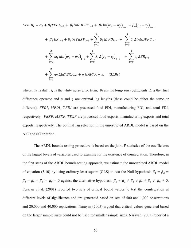
65

∆fSBTg = )J + IfSBTg +IhF!VB""8g +Ii lnO:o − :�Pg + IkOno − n�Pg+Im_`g + IpF!f_�"g +[∅��

�� ∆fSBTg� +[��J ∆F!VB""8g�

+[E��J ∆F!O:o − :�Pg� +[��

��J ∆Ono − n�Pg� +[L��J ∆_`g�

+[0��J ∆F!f_�"g� + eGSfG + jg�3.103�

where, )J is drift, jg is the white noise error term, I� are the long- run coefficients, ∆ is the first

difference operator and p and q are optimal lag lengths (these could be either the same or

different). SSBT, cSBT, fSBT are processed food FDI, manufacturing FDI, and total FDI,

respectively. S_�", c_�", f_�" are processed food exports, manufacturing exports and total

exports, respectively. The optimal lag selection in the unrestricted ARDL model is based on the

AIC and SC criterion.

The ARDL bounds testing procedure is based on the joint F-statistics of the coefficients

of the lagged levels of variables used to examine for the existence of cointegration. Therefore, in

the first steps of the ARDL bounds testing approach, we estimate the unrestricted ARDL model

of equation (3.10) by using ordinary least square (OLS) to test the Null hypothesis I = Ih =Ii = Ik = Im =Ip = 0 against the alternative hypothesis I ≠ Ih ≠ Ii ≠ Ik ≠ Im ≠Ip ≠ 0.

Pesaran et al. (2001) reported two sets of critical bound values to test the cointegration at

different levels of significance and are generated based on sets of 500 and 1,000 observations

and 20,000 and 40,000 replications. Narayan (2005) argued that critical values generated based

on the larger sample sizes could not be used for smaller sample sizes. Narayan (2005) reported a

66

new set of critical values for sample sizes ranging from 30 to 80. For the present study, we use

critical values from Narayan (2005). If the computed F-statistics are higher than the upper bound

critical values, then the null hypothesis of no cointegration is rejected and is classified as a long-

run relationship. Conversely, if the F-statistics are lower than the lower bound critical values,

then the null of no cointegration is not rejected. The results are inconclusive if the computed F-

statistics fall within the bounds for the critical values.

Once the long-run relationship was established in equation (3.10), we moved on to the

second step where the long- run coefficient based on the ARDL (p1, q1 q2 q3 q4) is estimated. The

lag length of the ARDL (p1, q1 q2 q3 q4 q5) can be selected based on AIC and SC criteria.

SSBTg = )J + [ I��D�� SSBTg� +[ Ih��D

��J F!VB""8g� + [ Ii��¢��J F!O:o −:�Pg�

+ [ Ik��£��J Ono − n�Pg� + [ Im��¤

��J _`g� + [ Ip��¥��J F!S_�"g� + eGSfGg

+jg�3.11@�

cSBTg = )J + [ I��D�� cSBTg� +[ Ih��D

��J F!VB""8g� + [ Ii��¢��J F!O:o − :�Pg�

+ [ Ik��£��J Ono − n�Pg� + [ Im��¤

��J _`g� + [ Ip��¥��J F!c_�"g� + eGSfGg

+jg�3.11y�

67

fSBTg = )J + [ I��D�� fSBTg� +[ Ih��D

��J F!VB""8g� + [ Ii��¢��J F!O:o − :�Pg�

+ [ Ik��£��J Ono − n�Pg� + [ Im��¤

��J _`g� + [ Ip��¥��J F!f_�"g� + eGSfGg

+jg�3.11y�

In the third step, we obtained short-run coefficients by estimating an error correction

model associated with the long- run estimates. The model is specified as follows:

∆SSBTg = t + [ ∅�∆��D�� SSBTg� +[ ��∆��D

��J F!VB""8g� + [ E��¢��J ∆ lnO:o − :�Pg�

+ [ ��£��J ∆Ono − n�Pg� + [ L�∆��¤

��J _`g� + [ 0��¥��J ∆F!S_�"g� + ¦_8cg

+jg�3.12@�

∆cSBTg = t + [ ∅�∆��D�� cSBTg� +[ ��∆��D

��J F!VB""8g� + [ E��¢��J ∆ lnO:o − :�Pg�

+ [ ��£��J ∆Ono − n�Pg� + [ L�∆��¤

��J _`g� + [ 0��¥��J ∆F!c_�"g� + ¦_8cg

+jg�3.12y�

68

∆fSBTg = t + [ ∅�∆��D�� fSBTg� +[ ��∆��D

��J F!VB""8g� + [ E��¢��J ∆ lnO:o − :�Pg�

+ [ ��£��J ∆Ono − n�Pg� + [ L�∆��¤

��J _`g� + [ 0��¥��J ∆F!f_�"g� + ¦_8cg

+jg�3.123� where ECM, the error term which is obtained from the equation (3.11) _8cg =SSBTg − )J −∑ I��D�� SSBTg� −∑ Ih��D��J F!VB""8g� −∑ Ii��¢��J lnO:o − :�Pg� −∑ Ik��£��J Ono −n�Pg� −∑ Im��¤��J _`g� − ∑ Ip��¥��J F!S_�"g� − eGSfGand _8cg is the one lagged of

the error correction terms. Here ∅�, ��, E�, ��, L�, and 0�are the short- run coefficients of the

model and coefficient (¦) associated with ECM allows for adjustment back to the long- run

equilibrium, given a deviation in the last quarter ( after a short-run shock).


3.4.1 Unit Roots Test

For ARDL bounds testing, pre-testing of the series for the order of integration is not required but

a unit root test was run to eliminate the possibility of I(2) or higher order of integration. In the

presence of I(2) variables, the computed F-statistics by Pesaran et al. (2001) and Narayan (2005)

are not valid. Therefore, to ascertain the order of integration, we applied ADF and PP unit root

tests in the level and the first differences of the series (Table 3.1). The results from the ADF test

do not reject the null hypothesis of non-stationary for all variables. At the same time, PP tests

also do not reject the null of non-stationary for all variables except, for the wage and exchange

rate (without trend). Once the tests are performed for the variables in their first differences, the

69

Table 3.1 ADF and PP unit root tests

Constant with trend Constant without trend

Variables ADF PP ADF PP

FFDI -2.44(3) -1.81(3) -2.41(3) -1.97(3)

MFDI -3.11(3) -2.83(3) -0.99(3) -1.47(3)

TFDI -2.78(3) -2.80(3) -2.40(3) -2.78(3)

lnGDPPC -1.95(2) -2.01(3) -0.28(2) -0.30(3)

ln(wd-wf) -1.70(3) -4.40(3)*** -2.55(3) -4.46(3)***

( rd-rf) -1.67(4) -2.20(3) -1.10(4) -1.72(3)

ER -2.79(1) -2.75(3) -2.80(1)* -2.86(3)**

lnFEXP -0.14(3) -1.41(3) -2.59(3) -2.06(3)

lnMEXP -2.53(3) -2.72(3) -1.49(3) -1.49(3)

lnTEXP -2.20(3) -2.53(3) -1.66(3) -1.64(3)

difference

∆FFDI -3.83(2)*** -3.12(3) -3.83(2)*** -3.09(3)**

∆MFDI -4.90(2)*** -4.48(3)*** -4.94(2)*** -4.56(3)***

∆TFDI -4.81(2)*** -4.23(3)*** -4.85(2)*** -4.34(3)***

∆lnGDPPC -6.34(2)*** -5.96(3)*** -6.36(1)*** -6.01(3)***

∆ ln(wd-wf) -5.49(2)*** -5.03(2)***

∆ ( rd-rf) -5.00(2)*** -6.98(3)*** -5.15(4)*** -7.01(3)***

∆ ER -7.85(1)*** -7.74(3)*** -7.83(0)*** -7.73(3)***

∆ lnFEXP -7.34(2)*** -4.22(3)*** -6.39(2)*** -4.07(3)***

∆ lnMEXP -5.50(2)*** -4.01(3)*** -5.47(2)*** -4.02(3)***

∆ lnTEXP -5.45(2)*** -4.03(3)*** -5.36(2)*** -4.03(3)*** Note: Asterisks indicate significance at the 10 percent (*), 5 percent (**) and 1 percent (***) levels, respectively. The critical values for ADF and PP tests with a constant and a trend are -4.032, -3.45, -3.147 whereas with a constant but no trend are -

3.4386, -2.856, and -2.568 for 1, 5, 10, percent significance levels, respectively. Figures in parenthesis are standard errors

null hypothesis is strongly rejected by both tests except for FFDI (The PP test with trend does

not reject the null of non-stationary for FFDI in first differences). A main problem associated

with the ADF and PP tests is that they do not allow for the possibility of structural breaks in the

series. The Zivot and Andrews and Perron and Vogelsang unit root tests allow for a single

structural break. The null hypothesis is that the time series are non-stationary with a single break.

The results are reported in table (3.2). The Zivot and Andrews test suggest that wage and FFDI

are I(0) in levels and all others are I(0) in their first difference, except per capita GDP. The

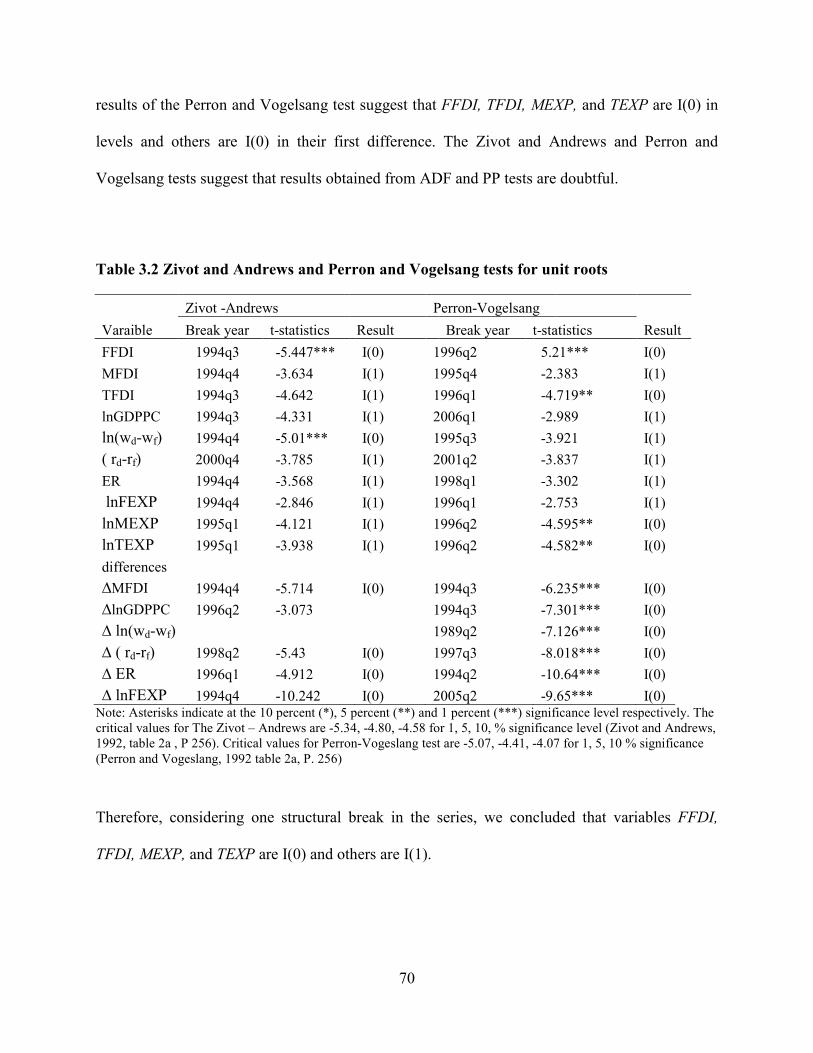
70

results of the Perron and Vogelsang test suggest that FFDI, TFDI, MEXP, and TEXP are I(0) in

levels and others are I(0) in their first difference. The Zivot and Andrews and Perron and

Vogelsang tests suggest that results obtained from ADF and PP tests are doubtful.

Table 3.2 Zivot and Andrews and Perron and Vogelsang tests for unit roots

Note: Asterisks indicate at the 10 percent (*), 5 percent (**) and 1 percent (***) significance level respectively. The critical values for The Zivot – Andrews are -5.34, -4.80, -4.58 for 1, 5, 10, % significance level (Zivot and Andrews, 1992, table 2a , P 256). Critical values for Perron-Vogeslang test are -5.07, -4.41, -4.07 for 1, 5, 10 % significance

(Perron and Vogeslang, 1992 table 2a, P. 256)

Therefore, considering one structural break in the series, we concluded that variables FFDI,

TFDI, MEXP, and TEXP are I(0) and others are I(1).

Zivot -Andrews Perron-Vogelsang

Varaible Break year t-statistics Result Break year t-statistics Result

FFDI 1994q3 -5.447*** I(0) 1996q2 5.21*** I(0)

MFDI 1994q4 -3.634 I(1) 1995q4 -2.383 I(1)

TFDI 1994q3 -4.642 I(1) 1996q1 -4.719** I(0)

lnGDPPC 1994q3 -4.331 I(1) 2006q1 -2.989 I(1)

ln(wd-wf) 1994q4 -5.01*** I(0) 1995q3 -3.921 I(1)

( rd-rf) 2000q4 -3.785 I(1) 2001q2 -3.837 I(1)

ER 1994q4 -3.568 I(1) 1998q1 -3.302 I(1)

lnFEXP 1994q4 -2.846 I(1) 1996q1 -2.753 I(1)

lnMEXP 1995q1 -4.121 I(1) 1996q2 -4.595** I(0)

lnTEXP 1995q1 -3.938 I(1) 1996q2 -4.582** I(0)

differences

∆MFDI 1994q4 -5.714 I(0) 1994q3 -6.235*** I(0)

∆lnGDPPC 1996q2 -3.073 1994q3 -7.301*** I(0)

∆ ln(wd-wf) 1989q2 -7.126*** I(0)

∆ ( rd-rf) 1998q2 -5.43 I(0) 1997q3 -8.018*** I(0)

∆ ER 1996q1 -4.912 I(0) 1994q2 -10.64*** I(0)

∆ lnFEXP 1994q4 -10.242 I(0) 2005q2 -9.65*** I(0)

71

3.4.2 ARDL Bounds Test Results

This section discusses the findings obtained from the ARDL bounds testing approach of Pesaran

et al. (2001). The analysis uses the outflows of FDI from the United States to Mexico for the

period 1988Q1 to 2008Q4. The first step in the ARDL bounds testing approach is to estimate

equation 3.10 using OLS regression. The optimal lag length in equation 3.10 is determined using

AIC and SC criteria. In order to select the optimal lag length, we set the maximum lag length of

4. The optimal lag of 2 is selected for total FDI. In selecting lag length for processed food and

manufacturing FDI, both AIC and SC criteria fail to provide conclusive results as to lag length.

For processed food FDI, the lag lengths of 2 and 1 are selected by AIC and SC criteria,

respectively. Similarly, for manufacturing FDI, lag lengths of 3 and 2 are selected by AIC and

SC criteria, respectively. To come up with the best fit for the model, the Ramsey RESET test for

the misspecification of the model was used. Therefore, we selected an optimal lag length of 2 for

both processed food and manufacturing FDI.

The misspecifications tests of equations 3.10 with or without NAFTA are reported in

Table (3.3). The regression for the ARDL equation fits the data very well explaining 96% of

variability in the dependent variable across the models’ independent variables (R2 = 96%). The

Breusch-Godfrey test (BG) results suggest the presence of serial correlation only in the total FDI

equation for the second lag, but the correlogram doesn’t indicate the presence of serial

correlation. All the equations pass the diagnostic tests of functional form misspecification,

normality, heteroscedasticitity, and autoregressive conditional heteroscedasticity. The cumulative

sum (CUSUM) and cumulative sum of squares (CUSUMQ) tests suggest that all the equations

satisfied the stability condition. We were then safe to test the existence of the long-run

relationship.

72

Table 3.3 Diagnostic tests for the ARDL equation

Without NAFTA With NAFTA

Tests FFDI MFDI TFDI FFDI MFDI TFDI

R2 0.97 0.97 0.96 0.97 0.97 0.96

BG1 1.52(0.21) 0.25(0.62) 2.28(0.13) 2.16(0.14) 2.06(0.15) 0.93(0.33)

BG2 3.438(0.18) 0.27(0.87) 2.50(0.29) 4.42(0.11) 4.03(0.13) 18.09(0.00)***

ARCH1 0.04(0.85) 0.06(0.81) 0.48(0.49) 0.07(0.79) 0.01(0.91) 0.28(0.56)

ARCH2 0.03(0.98) 0.07(0.96) 1.092(0.58) 0.08(0.96) 0.05(0.98) 0.38(0.83)

DW 2.13 2.05 2.08 2.17 2.17 2.07

WHITE 80(0.45) 80(0.45) 79(0.45) 80(0.45) 80(0.45) 79(0.45)

JB 3.50(0.17) 2.56(0.28) 5.66(0.06)* 5.05(0.08)* 1.25(0.53) 4.93(0.85)

RSEET 1.13(0.34) 1.66(0.19) 1.26(0.30) 0.74(0.53) 0.72(0.55) 1.17(0.33)

CUSUM satisfied satisfied satisfied Satisfied satisfied satisfied

CUSUMSQ satisfied satisfied satisfied Satisfied satisfied satisfied Note: Asterisks indicate at the 10 percent (*), 5 percent (**) and 1 percent (***) significance level respectively. Figures in parenthesis are probabilities. JB test is the Jarque-Bera test for normality; BG is the Breusch-Goldfrey test for autocorrelation based on lag 1 and 2. ARCH is test for autoregressive conditional heteroscedasticity of order 1 and 2.White is the White test for heteroscedasticity of the errors. RESET is the Ramsey RESET test, null is no specification problem. CUSUM, CUSUMSQ the cumulative sum of the recursive residual and the cumulative sum of squares of the recursive residual explains parameter instability if the cumulative sum or the cumulative sum of

square are not within the band of two critical lines at 5% significance level.

The results of the existence of long-run relationships are presented in Table (3.4).

Regression of the processed food FDI equation (3.10a) suggests that the F-statistics with or

without NAFTA (4.48 and 4.89) are higher than the upper bound critical value (3.864) at the 5%

significance level. The null hypothesis (i.e., no long-run relationship) is rejected for the

processed food FDI equation at the 5% level of significance. Regression of the manufacturing

FDI equation (3.10b) rejects the null hypothesis at the 1% level of significance in the presence of

NAFTA. The calculated F-statistics for the total FDI equation (3.10c) are higher than the upper

bound critical value at the 1% significance level. The existence of a long-run relationship is also

tested for export equations. The results suggest the existence of a long-run relationship for

processed food, manufacturing, and total export equations at the 1%, 10%, and 5% significance

levels, respectively.

73

Table 3.4 Results from bounds tests on equations 3.10 for the existence of a long-run

relationship

Dependent variables Lags Without NAFTA With NAFTA

FFDI 2 4.48** 4.89**

FEXP 2 6.21*** 5.49***

MFDI 2 4.65** 6.22**

MEXP 2 3.49* 3.42*

TFDI 2 4.95*** 6.22***

TEXP 2 4.22** 4.45** Note: Asterisks indicate at the 10 percent (*), 5 percent (**) and 1 percent (***) significance level respectively.

Asymptotic critical value bounds are obtained from Narayan (2005, p. 1989), Appendix: case III: unrestricted

intercept and no trend for k=6. Lower and upper bounds are 3.457- 4.943, 2.627-3.864, 2.236- 3.381 at 1%, 5%, and

10 % significance level respectively.

After the establishment of the existence of a long-run relationship, we estimated long-run

coefficients by applying OLS regression on equations (3.11 a, b, c). The appropriate lag length

for each variable on the ARDL is selected by AIC and SC criteria. Therefore, we estimated an

ARDL (2, 2, 2, 0, 0, 2) long–run model. The results are presented in table (3.5). The empirical

results on long-run coefficient estimations show that variables such as per capita GDP of

Mexico, real exchange rate, and lagged exports are very important variables to explain the U.S.

FDI inflows into Mexico. In our study, per capita GDP is a positive and highly significant

variable that explains FDI inflows into Mexico. This result is consistent with economic theory.

The U.S. company will normally invest in a country with greater market opportunities, which is

known as market-seeking FDI. With market-seeking FDI, the same type of capital will be

established in the foreign country. Many studies reported a positive relationship between

market-seeking FDI and GDP (Barrell and Pain, 1996; Barrell and Pain, 1997). Literature

focusing on Mexico (Love and Lage-Hidalogo, 2000; Thomas and Grosse, 2001) also supported

the positive relationship. The positive and statistically significant impact of per capita GDP on

74

U.S. FDI in the Mexican processed food sector is not surprising. For every 10 unit increase in

Mexican per capita GDP, FDI in the Mexican food sector increases by 0.011 % of GDP.

According to Regmi (2001), consumers in developing countries with higher income demand

more processed food. This demand for processed food increases with increases in income. The

positive relationship between market size and FDI in processed food is also found by Gopinath et

al. (1999); Mattson and Koo, (2002); Marchant et al. (2002); Makki et al. (2004).

There is a positive relationship between FDI and lagged exports (imports to Mexico).

This suggests complementary association between U.S FDI and U.S exports to Mexico. The

parameter estimate indicates that a 10 unit increase in U.S. exports to Mexico increases U.S. FDI

of processed food by 0.0020% of GDP (though the coefficient of U.S. exports is insignificant).

The complementary relationship could be due to the fact that FDI may cause producers to import

intermediate inputs from the home country. Therefore with an increase in outward FDI, exports

of the intermediate good increase (Banerjee 1997). The weak complementary relationship

between U.S. FDI and U.S. exports of processed food in Mexico could be due to a strong dollar

(Jerardo and Bolling, 2001; Bolling et al., 2007). The complementary relationship between

exports and FDI in the processed food sector is consistent with Merchant et al. (1999); Bolling

and Somwaru 2001; Mattson and Koo, (2002); Marchant et al. (2002). Studies such as Gopinath

et al. (1999) and Malanoski et al. (1997) dealt with the developed country cases and reported the

substitutionary relationship. The substitutionary relationship could possibly be because firms

may find it more cost effective to build a similar plant in the host countries rather than to export

(Malanoski et al., 1997).

There is a positive and highly significant relationship between FDI and U.S.

manufacturing exports to Mexico (imports to Mexico). This suggests a strong complementary

75

relationship between FDI and U.S exports of manufactured goods to Mexico. The parameter

estimates indicate that a 10 unit increase in U.S. exports of manufacturing leads to increased

inflows of FDI into Mexico by 0.051% of GDP. This finding is consistent with Lipsey and Weiss

(1981) who found a complementary relationship between U.S. exports of manufacturing and

FDI. In this study, we utilized majority U.S. controlled FDI (more than 50% of U.S. ownership),

Table 3.5 Estimated long- run coefficients using the ARDL (2,2,2,0,0,2) approach


Dependent FFDI MFDI TFDI FFDI MFDI TFDI

constant -0.29*** -4.94*** -4.90*** -0.30** -5.73***

-6.89***

(0.14) (1.37) (1.82) (0.15) (1.19) (1.68) lnGDPPC 0.11*** 1.58*** 2.47*** 0.11*** 1.82*** 2.78***

(0.04) (0.29) (0.39) (0.04) (0.25) (0.35) ln(wd-wf)

0.18*** 0.68*** 0.82*** 0.17*** 0.35* 0.42 (0.03) (0.21) (0.28) (0.04) (0.19) (0.27)

rd-rf (10-3)

0.10 -1.20 -2.36 0.09 1.02 -2.10 (0.60) (42.30) (5.56) (0.61) (3.66) (4.94)

ER 0.25*** -0.62 -0.29 0.25*** -0.46 -0.17 (0.07) (0.51) (0.62) (0.07) (0.44) (0.55)

lnFEXP 0.020 0.02 (0.017) (0.02)

lnMEXP 0.51*** 0.39** (0.18) 0.15

lnTEXP 0.21 0.08 (0.22) (0.20)

NAFTA(10-3) 0.04 6.40*** 8.11***

(0.25) (1.29) (1.86) Note: Asterisks indicate at the 10 percent (*), 5 percent (**) and 1 percent (***) significance level respectively.

Figures in parenthesis are standard errors.

therefore our finding is also consistent with the Pain and Wakelin (1998) who reported a

complementary relationship between majority U.S. owned FDI and exports of manufacturing for

OECD countries. There is a positive and insignificant relationship between FDI and total U.S.

76

exports suggesting a complementary association exists between total exports and total FDI. The

parameter estimates indicate that a 10 unit increase in total FDI exports leads to increased total

FDI investment in Mexico by 0.021% of GDP. Studies of Bajo-Rubio and Monter-Munoz, 2001;

Alguacil and Orts, 2002 indicate a complementary relationship between total FDI and U.S total

exports. Our finding is consistent with the literature.

The real exchange rate (home currency per host currency) is positive and statistically

significant for processed food FDI. An appreciation in the Mexican peso, relative to the U.S.

dollar, increases inflows of FDI into Mexico, which is not consistent with our hypothesis.

According to Waldkirch (2003), the positive association is also consistent with the argument that

the peso should appreciate if firm productivity increases as a result of capital inflows. Makki et

al. (2004) reported a negative relationship between real exchange rate and FDI in processed food

for developing countries. Other studies such as Bolling et al. (2007); Gopinath et al. (1998)

found that an appreciation of the U.S. dollar (depreciation of peso) increases outward FDI in

processed food indicating that countries with an undervalued exchange rate will experience an

increase in FDI. In other words, an undervalued Mexican peso will increase FDI inflows.

The real exchange rate is negative and insignificant for manufacturing and total FDI

inflows to Mexico. The result is consistent with our hypothesis, implying that appreciation of

peso (depreciation of U.S. dollar) decreases U.S. FDI to Mexico. As the U.S. dollar depreciates,

it will be more expensive for U.S. firms to invest in Mexico. Research findings regarding the

relationship between FDI and exchange rates are controversial. Some studies such as Froot and

Stein (1991); Görg and Wakelin (2002) suggested a negative relationship between host country

exchange rates and FDI. However, other studies (Blonigen, 1997; Campa, 1993; Waldkirch,

2003) reported a positive relationship between host country exchange rates and FDI.

77

The relative difference in wages between the U.S. and Mexico is positive and highly

significant in determining the level of FDI. Therefore, the result is consistent with our

hypothesis. This implies that an increase in U.S. wages increases FDI inflows into Mexico. For

every 10 dollar increase in the relative difference in wages, FDI in the Mexican processed food

sector increases by 0.018% of GDP, holding other factors constant. The finding is consistent

with literature (Love and Lage-Hidalgo, 2000; Skripnitchenko and Koo, 2005; Thomas and

Grosse, 2001). Some of the studies (Ning and Reed 1995; Matton and Koo, 2002) found a

negative impact of wages on FDI, suggesting that cheap labor may not be an important variable

in attracting FDI. The coefficient of interest rate is very small and insignificant for all types of

FDI, suggesting that user cost of capital is not an important variable to determine inflows of FDI

into Mexico, which is consistent with study of Love and Lage-Hidalgo (2000); Barrell and Pain

(1996).

The effect of NAFTA on the U.S FDI and U.S. exports to Mexico is another an important

part of this study. The effect of NAFTA was positive for all types of FDI suggesting that after

the implementation of NAFTA, FDI inflows into Mexico have increased. This finding is

consistent with our hypothesis. Interestingly, the lower impact of wages on FDI was observed,

even accounting for the effect of NAFTA. For manufacturing FDI, wage is significant only at the

10% level (it was significant at 1% before NAFTA) and even insignificant for total FDI. The

highly significant complementary relationship between FDI and exports of manufacturing is now

only significant at the 10% level. It seems that NAFTA had a devastating impact on the real

wage rate and on U.S exports to Mexico. Literature (Burfisher et al., 2001; Hoyos and Iacovone,

2011) suggests that it is very hard to disentangle the effect of NAFTA because at the same time

of NAFTA’s implementation (January, 1994), there was a Mexican financial crisis (December,

78

1994). Janvry (1996) argued that NAFTA greatly reduced the negative impact of the peso crisis

on U.S. trade with Mexico, which would have been extant in the absence of NAFTA. Audley et

al. (2004) stated that the lower impact of the wage variable was due to the pesos crisis and not to

NAFTA. This study’s finding of a weaker complementary relationship between FDI and U.S.

exports of manufacturing while taking into account NAFTA’s effect on U.S./Mexican trade is in

line with the above stated literature. A devaluation of the Mexican peso renders imports into

Mexico more expensive and thus brings about a weaker complementary relationship.

The results of short-run coefficients with long- run coefficients obtained from ECM are

given in table (3.6). However this time, the exchange rate is not significant for the processed

food FDI, intimating that exchange rates do not have significant short-run effects. The food

export, which is not significant in long-run coefficient estimation is now significant, suggesting

that a food export has a short run impact on processed food FDI. For manufacturing FDI,

variables such as exports, wage, and per capital GDP have short run effects. The error correction

term (equilibrium correction) coefficient is highly significant with the correct sign (negative),

implying a high speed of adjustment back to long-run relationship given a deviation in the

previous quarter (after a short-run shock). Approximately 51% of disequilibrium or shock from

the previous quarter converges back to the long- run equilibrium in the current quarter for the

processed food FDI. Higher speed of adjustment 77% and 89% were found for the

manufacturing and total FDI, respectively.

Some misspecification tests of the ARDL error correction model have been carried out

(table 3.7). The Breusch-Godfrey (BG) test results suggest serial correlation problem only in

total FDI equation. But the correlogram shows no problem of serial correlation. In addition, all

models satisfied the normality assumption. The Ramsey RESET tests show that there is not a

79

Table 3.6 Error correction representation for the selected ARDL (2,2,2,0,0,2) model


Dependent FFDI MFDI TFDI FFDI MFDI TFDI

constant -0.03 -0.56* -0.43 -0.03 -0.27 -0.06 (0.05) (0.28) (0.43) (0.05) (0.26) (0.41)

Ecm t-1 -0.51*** -0.77*** -0.89*** -0.50*** -0.84*** 0.81*** (0.14) (0.18) (0.25) (0.14) (0.14) (0.18)

∆FDI t-1 1.84*** 1.94*** 2.01*** 1.84*** 1.84*** 1.83*** (0.09) (0.14) (0.21) (0.09) (0.10) (0.14)

∆FDI t-2 0.99*** -1.00*** -1.07*** -0.99*** -0.92*** 0.90*** (0.08) (0.13) (0.19) (0.08) (0.09) (0.13)

∆lnGDPPC t 0.15*** 0.99*** 1.74*** 0.15*** 1.42*** 2.33*** (0.05) (0.31) (0.45) (0.05) (0.26) (0.42)

∆ lnGDPPC t-1 -0.34*** -2.88*** -4.09*** -0.35*** -3.50*** -4.61*** (0.08) (0.49) (0.80) (0.08) (0.46) (0.79)

∆ lnGDPPC t-2 0.27*** 2.47*** 2.94*** 0.27*** 2.49*** 2.69*** (0.05) (0.39) (0.65) (0.05) (0.33) (0.57)

∆ ln(wd-wf) t 0.17*** 1.35*** 1.59*** 0.17*** 0.78*** 0.84** (0.05) (0.28) (0.42) (0.05) (0.24) (0.38)

∆ ln(wd-wf)t-1 -0.24*** -1.93*** -2.51*** -0.24*** -1.07*** -1.32** (0.08) (0.47) (0.71) (0.08) (0.36) (0.58)

∆ ln(wd-wf)t-2 0.11*** 0.80*** 1.04*** 0.10*** 0.46** 0.56* (0.04) (0.22) (0.34) (0.04) (0.18) (0.29)

∆ rd-rf (10-3)t -1.17 7.38* 3.49 -1.18 8.58** 3.25 (0.76) (4.38) (6.54) (0.76) (3.95) (6.26)

∆ ER t 0.02 -0.64* -0.92 0.02 -0.55 -0.75 (0.06) (0.38) (0.56) (0.06) (0.34) (0.54)

∆lnEXP t 0.04* 0.57*** 0.30 0.04* 0.58*** 0.25 (0.02) (0.19) (0.27) (0.02) (0.17) (0.26)

∆lnEXP t-1 -0.06* -0.89*** -0.47 -0.06* -0.81*** -0.29 (0.03) (0.26) (0.38) (0.03) (0.23) (0.36)

∆lnEXP t-2 0.03 0.33*** 0.11 0.03 0.34*** 0.13

(0.02) (0.13) (0.22) (0.02) (0.12) (0.20) Note: Note: Asterisks indicate at the 10 percent (*), 5 percent (**) and 1 percent (***) significance level

respectively. Figures in parenthesis are standard errors

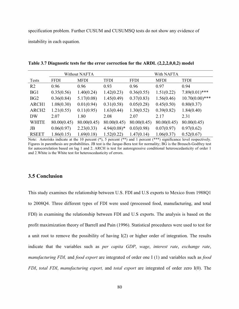
80

specification problem. Further CUSUM and CUSUMSQ tests do not show any evidence of

instability in each equation.

Table 3.7 Diagnostic tests for the error correction for the ARDL (2,2,2,0,0,2) model


Tests FFDI MFDI TFDI FFDI MFDI TFDI

R2 0.96 0.96 0.93 0.96 0.97 0.94

BG1 0.35(0.56) 1.40(0.24) 1.42(0.23) 0.36(0.55) 1.51(0.22) 7.89(0.01)***

BG2 0.36(0.84) 5.17(0.08) 1.45(0.49) 0.37(0.83) 1.56(0.46) 10.70(0.00)***

ARCH1 1.08(0.30) 0.01(0.94) 0.31(0.58) 0.05(0.28) 0.45(0.50) 0.80(0.37)

ARCH2 1.21(0.55) 0.11(0.95) 1.63(0.44) 1.30(0.52) 0.39(0.82) 1.84(0.40)

DW 2.07 1.80 2.08 2.07 2.17 2.31

WHITE 80.00(0.45) 80.00(0.45) 80.00(0.45) 80.00(0.45) 80.00(0.45) 80.00(0.45)

JB 0.06(0.97) 2.23(0.33) 4.94(0.08)* 0.03(0.98) 0.07(0.97) 0.97(0.62)

RSEET 1.86(0.15) 1.69(0.18) 1.52(0.22) 1.47(0.14) 1.06(0.37) 0.52(0.67) Note: Asterisks indicate at the 10 percent (*), 5 percent (**) and 1 percent (***) significance level respectively. Figures in parenthesis are probabilities. JB test is the Jarque-Bera test for normality; BG is the Breusch-Godfrey test for autocorrelation based on lag 1 and 2. ARCH is test for autoregressive conditional heteroscedasticity of order 1

and 2.White is the White test for heteroscedasticity of errors.

3.5 Conclusion

This study examines the relationship between U.S. FDI and U.S exports to Mexico from 1988Q1

to 2008Q4. Three different types of FDI were used (processed food, manufacturing, and total

FDI) in examining the relationship between FDI and U.S exports. The analysis is based on the

profit maximization theory of Barrell and Pain (1996). Statistical procedures were used to test for

a unit root to remove the possibility of having I(2) or higher order of integration. The results

indicate that the variables such as per capita GDP, wage, interest rate, exchange rate,

manufacturing FDI, and food export are integrated of order one I (1) and variables such as food

FDI, total FDI, manufacturing export, and total export are integrated of order zero I(0). The

81

ARDL bounds testing approach of Pesaran et al. (2001) was used to determine the relationship

between FDI and exports. This method is efficient in relatively small samples and our estimates

are also valid, even if some of the explanatory variables are endogenous. This procedure allows

for the inclusion of both I(0), I(1) or mixed variables. The order of lag is selected based on

Akaike Information Criteria (AIC) and Schwarz Criteria (SC). The bounds testing approach

suggests that variables in the profit maximization framework are bound together in the long-run.

The error correction terms have the expected signs (negative) and are highly significant, thus

suggesting a high speed of adjustment to the long-run equilibrium from short run shocks.

Empirical results indicate that per capita GDP, wage, and lag of exports measure market

size and are the most important variables in determining inflows of FDI into Mexico in the long-

run. The positive sign for per capita GDP is in line with market-seeking FDI literature (Barrell

and Pain 1996; Gopinath et.al., 1999; Matton and Koo, 2002). Results indicating that the real

exchange rate is both positive and significant with regard to processed food FDI are consistent

with the literature, suggesting that the host country’s currency should appreciate if a firm’s

productivity increases as a result of capital inflows (Waldkirch, 2003). The positive coefficient

of relative wage with FDI suggests that investment in Mexico is primarily due to lower labor

costs.

The most important finding of this research is the complementary relationship between

FDI and exports. The weak complementary relationship between FDI and exports of processed

food could be due to appreciation in the U.S. dollar. The appreciation of the dollar makes U.S.

exports more expensive for Mexican consumers. The highly significant and positive relationship

for manufacturing exports suggest that FDI in the manufacturing sector import raw inputs by

82

foreign affiliates to assemble final products. Most manufacturing products are re-imported into

the United States or exported to other countries.

The positive impact of NAFTA on all three types of FDI is another significant finding.

The impact of NAFTA is weak for processed food FDI. This could be due to the fact that there is

less volume in the international trade of the processed food than for FDI. The occurrence of the

pesos crisis with the implementation of NAFTA in the mid-1990s could be another factor. The

strong positive relationship of NAFTA with manufacturing FDI and total FDI suggest that after

the implementation of NAFTA, U.S foreign direct investment has been increasing to Mexico,

which is consistent with the goals of NAFTA. However, when accounting for the effect of

NAFTA on each of the FDI equations, the effect of wages on FDI decreases. The peso crisis can

be blamed for this finding too.

It is felt that further research with a larger sample size would improve the reliability of

the findings. It was also determined from the results of this study that the relationship between

FDI and their determinants vary with the level of aggregation of the firms, so firm level data

would be appropriate for the research to see the exact relationship. The research would also be

more informative if a Granger causality test of the relationship between FDI and trade could be

conducted.

3.6 References

Ajami, R. A. and BarNiv, R. (1984). Utilizing economic indicators in explaining foreign direct investment in the U.S. Management International Review 24(4): 16-26

Alguacil, M. T. and V.Orts (2002). Inward foreign direct investmetn and imports in Spain.

International Economic Journal 17(3): 19-38.

83

Amiti, M. and Wakelin, K. (2003). Investment liberalization and international trade. Journal of International Economics 61: 101-126.

Audley, J., Papademetriou, D., Polaski, S. and Vaughan, S. (2004).NAFTA's Promise and

Reality: Lessons from Mexico for the Hemisphere Carnegie Endowment for Int'l Peace. Bajo-Rubio, O. and Montero-Muñoz, M. (2001). Foreign Direct Investment and Trade: A

Causality Analysis. Open Economies Review 12(3): 305-323. Bajo-Rubio, O. and Sosvilla-Rivero, S. (1994). An econometric analysis of foreign direct

investment in Spain, 1964-89. Southern Economic Journal 61(1): 104-120. Barrell, R. and Pain, N. (1996). An Econometric Analysis of U.S. Foreign Direct Investment.

The Review of Economics and Statistics 78(2): 200-207. Barrell, R. and Pain, N. (1997). Foreign direct investment, technological chagne, and economic

growth within Europe. The Economic Journal 107(445): 1770-1786. Bevan, A., Estrin, S. and Meyer, K. (2004). Foreign investment location andinstitu tional

development in transition economies. International Business Review 13: 43-64. Blecker, R. A. (2007). The Economic Consequences of Dollar Appreciation for US

Manufacturing Investment: A Time-Series Analysis. International Review of Applied

Economics Volume 21, Issue 4, 2007 (4). Blonigen, B. A. (1997). Firm-Specific Assets and the Link between Exchange Rates and Foreign

Direct Investment. American Economic Review 87(3): 447-465. Blonigen, B. A. (2001). In search of substitution between foreign production and exports.

Journal of International Economics 53: 81-104. Bolling, C., Calderon, J. and Handy, C. (1999). U.S. frims invest in mexico's processed food

industry. Food Review 22(2): 26-30. Bolling, C., Shane, M. and Roe, T. (2007). Exchange rates and U.S. foreign direct investment in

the global processed food industry. Agricultural and Resource Economics Review 36(2): 230-238.

Bolling, C. and Somwaru, A. (2001). U.S. food companies access foreign markets through direct

investment. Food Review 24(3): 23-28. Burfisher, M. E., Robinson, S. and Thierfelde, K. (2001). The Impact of NAFTA on the United

States. Journal of Economic Perspectives 15(1): 125-144. Campa, J. M. (1993). Entry by Foreign Firms in the United States Under Exchange Rate

Uncertainty. The Review of Economics and Statistics 75(4): 614-622

84

Chakrabarti, A. (2001). The Determinants of Foreign Direct Investments: Sensitivity Analyses of

Cross-Country Regressions. Kyklos 54(1): 89–114. Coughlin, C. C., Terza, J. V. and Arromdee, V. (1991). State Characteristics and the Location of


Statistics 73(4): 675-683 Culem, C. G. (1988). The locational determinants of direct investments among industrialized

countries. European Economic Review 32(4): 885-904. Daniels, J. D., Krug, J. A. and Trevino, L. (2007). Foreign direct investment from Latin America

and the Caribbean. Transnational Corportations 16(1): 27-54. Engle, R. F. and Granger, C. W. J. (1987). Cointegration and Error Correction: Representation,

Estimation, and Testing. Econometrica 55(2): 251-276 Froot, K. A. and Stein, J. C. (1991). Exchange Rates and Foreign Direct Investment: An

Imperfect Capital Markets Approach. Quarterly Journal of Economics 106(4): 1191-1217.

Glodberg, L. G. and Grosse, R. (1994). Location choice of forein Banks in the United States.

Journal of Economic Business 46: 367-379. Gopinath, M., Pick, D. and Vasavada, U. (1998). Exchange rate effect on the realtionship

between FDI and trade inthe U.S. food processing industry. Agricultural and Applied Economics Association 80(5): 1073-1079.

Gopinath, M., Pick, D. and Vasavada, U. (1999). The economics of foreign direct investment and

trade with an application to the U.S. food processing industry. Agricultural and Applied Economics Association 81(2): 442-452.

Gorg, H. and Wakelin, K. (2002). The impact of exchag e rate volatility on US direct investment.

The Machester School 70(3): 380-397. Grosse, R. and Trevino, L. J. (1996). Foreign Direct Investment in the United States: An

Analysis by Country of Origin. Journal of International Business Studies 27(1): 139-155 Handy, C. R. and Henderson, D. R. (1994).Assessing the Role of Foreign Direct Investment in

the Food Manufacturing Industry. In Competitiveness In International Food Markets(Eds M. E. Bredahl, P. C. Abbott and M. C. Reed).

Harris, R. and Sollis, R. (2003). Applied Time Series Modelling and Forecasting. West Susse:

Wiley. Head, K. and Ries, J. (2001). Overseas Investment and Firm Exports. 9 1: 108-122.

85

Henderson, D. R., Handy, C. R. and Neff, S. A. (1996).Globalization of the processed foods

market,Agricultural Economic Report No. 742. Washington, DC: United States Department of Agricultural, Economic Research Service, Food and Consumer Economics Division.

Heston, A., Summers, R. and Ate, B. (2011).Penn World Table Version 7.0. Center for


Hoyos, R. E. D. and Iacovone, L. (2011).Economic Performance under NAFTA: A Firm-Level

Analysis of the Trade-Productivity Linkages,Policy Research Working Paper No 5661. The World Bank Development Research GroupTrade and Integration Team,May 2011.

IMF (2010).International Financial Statistics CD-ROM. IMF. Janvry, A. d. (1996).NAFTA and agricultural: An early assessment. In Working paper No 807:

Gianni Foundation University of California Berkley. Jerardo, A. and Bolling, C. (2001).U.S. processed food FDI and exports to Canada and Mexico:

an investigation into time-series relationhsip. In Paper presented at the AAEA Conference, Chicago, IL.

Johansen, S. and Juselius, K. (1990). Maximum likelihood estimation and inference on

cointegration: with application to the demand for money. Oxford Bulletin of Economics

and Statistics 52(2): 169-210. Kim, J.-D. and Rang, I.-S. (1997). Outward FDI and exports: The case of South Korea and

Japan. Journal of Asian Economics 8 (1): 39-50. Lipsey, R. E. and Weiss, M. Y. (1981). Foreign Production and Exports in Manufacturing

Industries. The Review of Economics and Statistics 63 (4): 488-494. Liu, X., Song, H., Wei, Y. and Romilly, P. (1997). Country characteristics and foreign direct

investment in China: A panel data analysis. Weltwirtschaftliches Archiv. 133 (2): 313-329.

Love, J. H. and Lage-Hidalgo, F. (2000). Analysing the determinants of US direct investment in

Mexico. Applied Economics 32: 1259-1267. Lütkepohl, H. and Krätzig, M. (2004). Applied Time Series Econometrics. New York:

Cambridge University Press. Makki, S. S., Somwaru, A. and Bolling, C. (2004). Determinants of foreign direct investment in

the food processing industry: A comparative analysis of developed and developing economes. Journal of Food Distribution Research 35(3): 61-66.

86

Malanoski, M., Handy, C. and Henderson, D. (1997).Time Dependent Relationship in U.S.

Processed Food Trade and Foreign Direct Investment. In Organization and Performance

of World Food Systems, Vol. 182(Ed S. R. Henneberry). Oklahoma State University. Marchant, M. A., N.Cornell, D. and Koo, W. (2002). International trade and foreign direct :

substitute or complement. Journal of Agricultural and Applied Economics 34(2): 289-302.

Marchant, M. A., Saghaian, S. H. and Vickner, S. S. (1999). Trade And Foreign Direct

Investment Management Strategies For U.S. Processed Food Firms In China. International Food and Agribusiness Management Review 2(2): 131-143

Mattson, J. W. and W.Koo, W. (2002).Processed food trade and foreign direct investmetn under

NAFTA. Fargo, North Dakota: North Dakota State University Center for Agricultural Policy and Trade Studeis department of Agribusiness and Applied Economics Agricultural Experiment station.

Mundell, R. A. (1957). International trade and factro mobility. American Economic Review 47:

321-335. Narayan, P. K. (2005). The saving and investment nexus for China: evidence from cointegration

tests. Applied Economics 37(17): 1979-1990. Newey, W. K. and West, K. D. (1994). Automatic Lag Selection in Covariance Matrix

Estimation. Review of Economic Studies 61 (4): 631-653. Ning, Y. and Reed, M. R. (1995). Locational determinants of the US direct foreign investmetn in

food and kindred products. Agribusiness 11(1): 77-85. Pain, N. and Wakelin, K. (1998). Export Performance and the Role of Foreign Direct Investment.

The Manchester School of Economic and Social Studies. 66(0): 62-88. Pan, Y. (2003). The inflow of foreign direct investment to China:the impact of country-specific

factors. Journal of Business Research 56: 829 – 883. Peasaran, M. H. and Shin, Y. (1999).An autoregressive distrubited lag modeling approach to

cointegration analysis. In Econometrics and economic theory in the 20th century:The

Ranger Frisch centennial symposium(Ed S. Strom). Cambridge University Press. Perron, P. and Vogelsang, T. J. (1992). Nonstationarity and level shifts with an application to

purchasing power parity. Journal of Business and Economic Statistics 10(3): 301-320. Pesaran, M. H., Shin, Y. and Smith, R. J. (2001). Bonds testing approaches to the analysis of

level relationship. Journal of Applied Econometric 16(3): 289- 326.

87

Pfaffermayr, M. (1996). Foreign outward direct investment and exports in Austrian manufacturing: Substitutes or complements? Review of World Economics 132(3): 501-522.

Reed, M. R. and Marchant, M. A. (1992). The global competitiveness of the U.S. food-

processing industry. Northeastern Journal of Agricultural and Resource Economic 21(1): 61-70.

Regmi, A. (2001).Changing Structure of Global FoodConsumption and Trade:An Introduction.

In Changing Structure of Global Food Consumption and Trade: Economic Research Service, USDA.

Regmi, A. and Gehlhar, M. (2005).New directions in global food markets. In Agriculture

Information Bulletin: United States Department of Agriculture. Skripnitchenko, A. and Koo, W. W. (2005). U.S. foreign direct investmetn in food processing

industries of Latin America countries: a dynamic approach. Review of Agricultural

Economics 27(3): 394-401. Somwaru, A. and Bolling, C. (1999).U.S. foreign direct investmetn and trader: substitutes or

complements? the case of the food processing industry. In American Agricultural

Economics Association Annual MeetingNashville, TN. Thomas, D. E. and Groose, R. (2001). Country-of-origin determinants of foreign direct

investment in an emerging market: the case of Mexico. Journal of International Mangement 7: 59-79.

UNCTAD (2002).World Investement Report 2002: Transational Corporations and Export

Competitiveness. New York: United Nations. Waldkirch, A. (2003). The 'new regionalism' and foreign direct investment: the case of Mexico.

Journal of International Trade and Economic Development 12(2): 151-184. Waldkirch, A. (2008). The Effects of Foreign Direct Investment in Mexico since NAFTA. The

World Economy 33(5): 710-745. Wilkinson, J. (2008).The Food Processing Industry, Globalization and Developing Countries. In

The Transformation of Agri-Food Systems:Globalization, Supply Chains and Smallholder

Farmers(Eds E. B. McCullough, P. L. Pingali and K. G. Stamoulis). Worth, T. (1998).Regional Trade Agreements and Foreign Direct Investment. In Regional Trade

Agreements and U.S. Agriculture: Economic Research Service/USD. WTO (2001).International trade statisics 2001.

88

Zivot, E. and Andrews, D. W. K. (1992). Further Evidence on the Great Crash, the Oil Price Shock, and the Unit Root Hypothesis. Journal of Business and Economic Statistics 10: 251-270.

89

Chapter 4: Relationship among Foreign Direct Investment, Economic Growth

and Exports in Mexico

4.1 Introduction

In developing countries, foreign direct investment (FDI) is a main channel through which capital,

knowledge, and technologies are transferred between countries. The benefits from FDI on

economic growth depend upon the ability of the host countries to access, learn, and implement

new technologies (Borensztein et al., 1998; Waldkirch, 2010; Xu, 2000). According to Bhagwati

(1978), the benefits from FDI are likely to be less if FDI is a substitute for imports in comparison

to countries with export promotion policies. Thus, the growth enhancing effect of FDI and trade

interaction depends upon the specific policies and factor endowments of various countries.

The relationships among FDI, exports, and economic growth have been explored quite

extensively in economic literature. The majority of research has used a bivariate framework.

Studies that used bivariate framework include: Baliamoune-Lutz (2004); Sharma and

Panagiotidis (2005); Xu (1996). Meanwhile, other researchers such as Balassa (1978);

Balasubramanyam et al. (1996); Feder (1983); Fosu (1990); Tsai, (1994) used a multivariate

framework derived from the production function, in which the growth variable is regressed

against exports or FDI along with other endogenous variables such as labor and capital. The

growth hypothesis is supported if the coefficient on export/ FDI is significantly positive. Most

cross-country studies assume a positive relationship between FDI and economic growth (FDI-led

growth) (Balasubramanyam et al., 1996; Borensztein et al., 1998). According to

Balasubramanyam et al. (1996), there is a strong role of FDI on economic growth in export

promoting countries in comparison to the countries with import-substitution policies. Similarly,

most of the research shows a positive relationship between economic growth and exports

90

(export-led growth) in cross-country studies (Balssa, 1984; Feder 1983; Fosu 1996). However,

the major problem or limitation of cross-country data analysis is the assumption of common

production technologies across countries, which is not always true4. The host countries’ domestic

policy such as monetary, fiscal, production technology, financial structures, and external shocks

may differ across countries. Therefore, the effect of FDI and exports on growth varies across

countries. Further, provision for the case of reverse causality was not allowed in past research,

which has led to inconsistent conclusions.

There is ample research literature (Apergis et al., 2008; Choe, 2003; Liu et al., 2001) on

panel and time series data for individual countries, using methods that allow reverse causality

between a pair of variables in a bivariate or in a multivariate framework. Some empirical studies

(Basu et al., 2003; Choe 2003; Karikari 1992; Liu et al., 2002; Pradhan, 2009) show a

bidirectional causality between FDI and growth. In a relatively open economy, Apergis et al.

(2008) found a two-way causal relationship between FDI and economic growth. Some studies

(Chakraborty and Basu, 2002) reported a one-way causality from GDP to FDI. In a closed

economy, Basu et al. (2003) reported a one-way causality flow from GDP to FDI. Research

studies (Awokuse, 2005; Awokuse, 2006; Maneschiold 2008) reported the two-way causality

between exports and growth. However, studies such as Awokuse (2003) suggested a one-way

causality running from exports to growth. Meanwhile, Sharma and Panagiotidis (2005) reported

a no causal relationship between exports and growth.

Research results on causal relationships among exports, FDI, and GDP are contradictory

with results ranging from unidirectional causality, bidirectional causality or no causality at all. In

this study, we explore in depth the issue of exports, FDI, and GDP. The main purpose of this

4In other words, these studies do not take into account the level of technology.

91

research is to examine the direction of causality among FDI, exports, and growth using time

series data from the Mexican economy. Toda and Yamamoto (1995) and Dolado and Lukepohl

(1996) -TYDL- methodology is used to test the direction of causality between a pair of variables.

We also investigated the impact of NAFTA and United States GDP on causality among

variables. This study aims to shed light on the mixed results of Granger causality among FDI-led

growth, export-led growth, and FDI-led exports by constructing a five variable vector auto

regressions (VAR) model for Mexican economic growth. Annual time series data from 1970 to

2008 were used for the analysis.

4.1.1 Economic Growth in Mexico

Mexico is the largest FDI recipient in Latin America (UNCTAD, 2002) and, among developing

countries, is the second largest trading country (by volume) in the world (WTO, 2001). The

economic growth of Mexico was interrupted by several economic factors such as oil shocks,

fiscal and monetary policies, debt crisis, and devaluation of the Mexican peso. The annual

economic growth rate of Mexico was 4.1 % from 1961 to 2009 and 6.7% per year for the years

1961 to 1970. The economic growth rate in the Mexican economy began to slow down in the

1970s, primarily due to crude oil price shocks and a slowdown in overall productivity. The

macroeconomic changes that occurred during the mid-1970s led to a debt crisis in the early

1980s and a sharp recession in GDP growth. From 1981 to 2009, annual average GDP growth

slumped to 2.29 %. Implementation of NAFTA in 1994 seems to have had a positive impact on

the economic growth of Mexico, but the economic crisis resulting from the devaluation of the

peso at the same time led to decreased output and a significant rise in inflation. After recovery

from the peso crisis, the annual growth rate increased by 2.84% from 1996 to 2009 (Figure 4.1).

92

Figure 4.1 GDP and Exports growth rates (percent), 1960 to 2009 Source: World Develoment Indicator online version, World Bank (2011).

In several studies, researchers argued that exports are the main channel through which the

trade liberalization can effect economic growth (Balassubramanyam et al., 1996). It was

observed that the effect of export substitution policies on economic growth had less impact than

import substitution policies. The average growth rate of exports before 1980 was 8.169% per

year. The average export growth rate changed to 8.64% after the shift from an import

substitution policy to an export promotion policy. In 1986, Mexico joined the GATT which

reduces tariffs and relaxes restrictions on foreign investments in an economy. The annual export

growth rate was 8.6% from 1980-1993. Exports increased dramatically after 1994. Between

1994 and 2008, the export growth rate was 10.24%. Export growth slumped dramatically in

2009 due to the economic crisis in the United States (Figure 4.2).

-20

-10

01

02

03

0P

erce

nt

1960 1970 1980 1990 2000 2010year

real GDP growth real export growth

93

Figure 4.2 FDI inflows into Mexico (percent of GDP), 1970 to 2009 Source: World Develoment Indicator online version, World Bank(2011)

The foreign investment law (FIL) in Mexico was first introduced in 1973 and FDI was

ratified only for a specific proportion of a firm’s total capital such as mining (only 49%),

petrochemical (40%), and fabrication of automobile components (40%) (UNCTAD, 1992).

After the debt crisis, the FIL was modified in 1989, allowing for 100% ownership of a firm’s

capital in many sectors. The changes were also made in 1993 to make FIL compatible with

NAFTA. Another policy change was made in 1999, allowing for the liberalization of a majority

of financial services. The inflow of FDI in Mexico during 1980 and 1990 was 1.14% of GDP.

One of the principal aims of NAFTA was to increase U.S. FDI inflows in Mexico and the results

thereafter have been 2.89% of average GDP (Figure 4.2).

01

23

45

Per

cent

of

GD

P

1960 1970 1980 1990 2000 2010Year

FDI as percent of GDP

94

4.2 Literature Review

The causality relationship in the cross-country study assumes a positive relationship between

FDI and growth as well as exports and growth (Balasubramanyam et al., 1996; Balssa, 1985;

Borensztein et al., 1998; Feder 1983; Fosu, 1996). The major limitation of the cross-country

study is the assumption of a similar production function across all countries. Recent

developments in econometric analysis of panel and time series data and the more sophisticated

econometric methods resulting from extended research allowed researchers to examine the

reverse causality test among different economic variables. The following research articles

provide causality in Panel and individual country cases using time series data.

4.2.1 Granger Causality Studies on Panel Data

Choe (2003) examined Granger causality between FDI and economic growth for 80 countries

from 1971-95 by using a panel VAR model. The research results suggest a bidirectional causality

between FDI and economic growth. Using panel cointegration and the panel causality test,

Apergis et al. (2008) report a positive impact of FDI on economic growth for high income

countries that have successfully implemented privatization programs. Basu et al. (2003)

examined the relationship between FDI and GDP using cointegration and causality over the

period 1978-1996. Results suggest a two-way causality between FDI and growth for relatively

open economies and a one-way causality for closed economies. Using panel cointegration

analysis, Pradhan (2009) explored the relationship between FDI and economic growth of

ASEAN countries from 1970-2007. Except for Malaysia, the study shows a bidirectional

causality between FDI and economic growth, suggesting that a high level of FDI can generate a

corresponding high level of economic growth. High levels of economic growth can, in turn,

95

generate high levels of FDI. Using multivariate Granger causality in a VAR format, Liu et al.

(2001) examined the causal relationship among FDI, exports, and imports in China using panel

data over the period of 1984-1998. Researchers suggested a positive causal relationship from

imports to FDI, FDI to exports, and exports to imports.

4.2.2 Granger Causality Studies on Individual Countries

Several studies examine the Granger causality effect on individual countries. While analyzing

the causality effect, some studies used bivariate while others have used multivariate frameworks.

Karikari (1992) examined bivariate causality between FDI and growth in Ghana for the period

from 1961 to1988, without considering integration and cointegration. The research results do not

support the hypothesis of causality between FDI and growth. Using the technique of

cointegration and error correction modeling (VECM), Chakraborty and Basu (2002) explored the

link between FDI flows and economic growth in India under a multivariate framework. Results

suggest that the direction of causality runs from GDP to FDI.

Sharma and Panagiotidis (2005) formulated the model based on Feder’s (1983) to test the

Granger causality effect on multiple economic variables. The results do not support causality

between a pair of variables such as export and growth; export and investment; export and gross

fixed capital formation; and so on. Alguacil and Orts (2002) explored VECM in Spain using

quarterly data for the period 1970-1992 and reported a one-way causality running from FDI to

exports. Baliamoune-Lutz (2004) examined the relationship between exports, FDI, and growth in

Morocco using data from 1973 to 1999. The research results suggest two-way causal

relationships between FDI and exports, a one-way causal relationship running from FDI to

growth, and a one-way causality running from exports to growth.

96

Based on the new growth theory, Shan and Sun (1998) applied Toda and Yamamoto

(1995) and Doland and Lukepohl (1996) (TYDL) methodologies to test the export- led growth

hypothesis in China since 1987 to 1996. The results indicate a two-way causality between

exports and growth. A bidirectional causal relationship among FDI, growth, and exports in

China is also reported by Liu et al. (2002) using quarterly data from 1981 to 1997. Dritsaki et

al. (2004) examined the relationship between exports, economic growth, and foreign direct

investment for Greece using annual data for the period 1960-2002 and the VAR error correction

method. The study suggested two-way causal relationships between exports and economic

growth. The study also shows a unidirectional causal relationship of FDI on GDP. Awokuse

(2003) tested the export-led growth hypothesis based on the augmented production function for

Canada using VECM and TYDL causality testing methods. Quarterly data from 1961 to 2000

were used. In this study, a one-way causality running from exports to growth was observed.

Using similar method and quarterly data from 1963 to 2001, Awokuse (2005) also examined the

export-led growth for Korea. The research findings show a two-way causality between exports

and growth.

Using quarterly data from 1990 to 2002 and TYDL methodology, Duasa (2007) tested the

causal relationship between FDI and growth in Malaysia. The study does not support the causal

link between FDI and economic growth. Omisakin (2009) used data from 1970-2006 and TYDL

and autoregressive distributed lag (ARDL) models to examine the causal relationship among

FDI, growth, and trade openness in Nigeria. The results reveal unidirectional causality running

from FDI to growth. Ericsson and Irandoust (2001) examined the causal relationship between

FDI and growth for four OECD countries: Denmark, Finland, Norway, and Sweden. This study

was based on a production function framework for the period of 1970 to 1997. The results

97

supported bidirectional causality between FDI and growth for Sweden and unidirectional

causality running from FDI to growth for Norway. Using the neoclassical growth theory and

multivariate cointegration VAR, Awokuse (2006) tested the export-led growth and import-led

growth separately for Bulgaria, the Czech Republic, and Poland. The researcher found evidence

of a two-way causality between exports and growth. The research findings also indicate a one-

way causality running from exports and imports to growth for the Czech Republic and imports to

exports for Poland.

4.2.3 Granger Causality Studies in Mexico

Numerous studies also examined the relationship between FDI, exports, economic growth, and

other major economic variables for Mexico. Thornton (1996) carried out the bivariate causality

test using cointegration over 1895-1992. The study found a positive relationship flowing from

exports to economic growth. This research result is also supported by Abdulnasser and

Manuchehr (2000). Alguacil et al. (2002) analyzed the causality between exports, FDI, and

domestic performance using time series data from 1980.I to 1999.IV in Mexico. The results

support both the export-led growth and FDI-led growth hypothesis. Cuadros et al. (2004) found

a positive FDI-led growth in Mexico using the TYDL procedure for the period 1980.I to

2000.IV. Maneschiold (2008) analyzed the export-led growth hypothesis for Argentina, Brazil,

and Mexico using a VAR error correction framework. The study showed a two-way causality

between exports and growth after the inception of NAFTA and a one-way causal relationship

flowing from exports to GDP before the inception of NAFTA.

The above literature review shows three different frameworks (cross country, panel, and time

series) to study growth nexus. Panel cointegration is the most recent technique to have been

98

developed that deals with the country specific cointegration relationship. According to Banerjee

et al. (2004), the cointegration test in panel data may be falsely rejected (null of no cointegration)

due to few cointegrated relationships. Thus, the causality literature using panel data may be

misleading. He suggested looking at the relationships on a country by country case. Further, the

past literature also shows that the causality relations differ with the period of study, country, and

methods of econometric analysis. Empirical evidence is mixed and inconclusive.

Therefore, this study will investigate the long-run relationship among FDI, growth, and

exports. In this analysis, we attempt to test first the hypothesis that FDI improves the economic

growth of the host country (FDI-led growth) ; secondly, the hypothesis that exports improve

economic growth of the host country (export-led growth); thirdly, the hypothesis that the

economic growth of the host country improves the growth of FDI (export-led FDI); fourthly,

the hypothesis that FDI improves the growth of exports (FDI-led export); fifthly, the hypothesis

that exports improve growth in FDI (export-led FDI); sixthly, the hypothesis of bidirectional

causality or possibly the case of no causality at all. Theoretical and empirical models to test

these hypotheses are developed in section 4.4. Empirical results are presented in the section 4.5.

The last section summarizes the conclusions of the chapter.


4.3.1 The Model

The model to investigate interrelationships among FDI, economic growth, and exports is derived

from a production function in which FDI is introduced as an input, in addition to labor and

capital. Suppose the level of output in an economy is determined by the production factors and

the production technology as shown below:

99

§g = Gg\g∝lg̈ �4.1� where, §g stands for gross domestic product (GDP), K and L for the inputs of capital stock and

labor stock, respectively, all in year t. The variable A is used to denote total factor productivity

(TFP). TFP is the amount of output that is not explained by increasing labor or capital inputs. We

assume that the coefficients of K, L, and A are positive. Thus, assuming constant technology, any

rise in the amount of labor or capital will increase the output level in that economy. The

production function described in equation 4.1 is expanded according to a new growth theory

mentioned by Barro and Sala-i-Martin (1995) and Fosu (2006).

Improvements in technology (e.g. improved capital stock) makes labor more productive

and increases per worker output with fixed supplies of both labor and capital. Chen (1992) and

Borensztein et al. (1998) argue that foreign direct investment (FDI) is a major source of human

capital and new technology in developing countries. According to Lipsey (2001), the impact of

FDI on economic growth is through TFP. The inclusion of FDI in a production function will

capture externalities such as learning by watching and spill-over effects. The impact of FDI and

other relevant variables can be captured through A. Equation 4.1 can be written as follows:

§g = _g\g∝lg̈SBTg©�4.2� where E represents exogenous factor of growth. The importance of exports for economic growth

has been well documented in economic literature and several researchers have counted exports in

their production functions. Several examples of literature explaining the export–led growth

hypothesis (Abu-Quarn and Abu Bader, 2004; Ericcson and Irandoust, 2001; Thornton, 1996)

showed the importance of exports in economic growth. According to Fosu (1990), exports are

viewed as the systematic error term affecting output. This will secure the effect of the

100

international factors influencing the output that is not secured by either labor or capital. Riezman

et al. (1996) have pointed out that Granger causality tests may be misleading if imports are not

counted in the production function. We included a dummy variable NAFTA to take into account

the effect of trade liberalization (NAFTA = 1 from 1994 to 2008 and zero otherwise). In Mexico,

a majority share of FDI flows from the United States. In addition, the geographic proximity of

Mexico to the United States combined with the existence of several other trade agreements

between Mexico and the United States serve to interconnect the Mexican economy with that of

the United States. Hence, the GDP of the United States has been included in the growth equation

to secure against foreign economic shocks. To investigate the causal relationship among FDI,

exports, and growth along with the capital and labor, equation (4.2) can be written as follows:

§g = _g\g∝lg̈SBTg©TQ$xnYgª_�$xnYg=fnb!�gCeGSfGg∅�4.3� From equation (4.2) it can be written as follows:

F!§g = 8+∝ F!\g + IF!lg + LF!SBTg + «F!TQ$xnYg +;F!_�$xnYg + ∅eGSfGg+bg�4.4�

F!§g = 8+∝ F!\g + IF!lg + LF!SBTg + «F!TQ$xnYg +;F!_�$xnYg + Efnb!�+ 0F!�HVB"g +bg�4. 5�

where ln represents the natural logarithm of the variables and bg is white noise and is assumed to

be normally and identically distributed, C is the constant term. The log linear specification

implies that the parameters ∝, I, L, «, ;, and 0are elasticities of capital, labor, FDI, imports,

exports, and GDP of the United States, respectively. The sign of the parameters are all expected

to be positive.

101

4.3.2 Data

This research uses annual time series data for Mexico from 1970 to 2008. Aggregate output (Yt)

is measured by real GDP of Mexico and Mexican capital stock (Kt) is proxied by the real value

of gross fixed capital formation (GFCF). This proxy for capital stock has been used in several

studies such as Balsubramanyam et al. (1996) and Borensztein et al. (1998). The data on labor

(Lt) corresponds to the number of economically active citizens in the Mexican population.

Foreign direct investment was converted to real FDI using the GDP deflator for Mexico (in 2000

constant prices). All data were converted into natural logarithms before analysis. The data

sources for all variables were the World Development Indicator (WDI, 2011) and the Penn

World Tables (Appendix 4.1). The summary statistics is provided in Appendix 4.2

4.4.3 Econometric Methods

The majority of time series studies have used the Granger causality test to examine the causality

between economic variables. The concept of causality was initially defined by Granger (1969) in

a bivariate framework. A time series X is said to be the ‘Granger cause’ of a series Y. If the

connection can be made that shows through a series of t-tests and F- tests on the values of X that

have been lagged, than those lagged X values furnish information about future values of Y that

are statistically significant.

The standard Granger causality tests are sensitive to the model selection and functional

form. As far as the model specification is concerned, most of these studies have used simple two

variable relationships (Gujaratio, 1995 Gujaratio, 1995; Xu, 1996). Sims (1972) argued that

Granger causality in a bivariate model is mainly due to the omitted variable. In such cases the

102

causal inferences are invalid, the Granger causality test requires that the underlying variables

must be stationary (Granger, 1988).

The Engle and Granger correction model (ECM) as developed by Engle and Granger

(1987) and the vector autoregressive error correction model (VECM) as developed by Johansen

and Juselius (1990) are just two examples of recent developments in time series analysis that

consider the issue of integration and cointegration in time series analysis. In these models, the

error correction term describes the long-run equilibrium relationship and the lagged difference

terms indicate the short-run relationship. Both ECM and VECM specifications are cumbersome

and sensitive to values of nuisance parameters, especially in the case of small sample size

(Rambaldi and Doran, 1996). To determine the extent of cointegration, the Engle and Granger

method uses the Augmented Dickey-Fuller (ADF) test on the residuals obtained from the

regression on the level variables. This may give inefficient and misleading results if more than

two I(1) variables are used in the regression and the nature of the variables are endogenous5. The

VECM process allows for a multivariate format and also allows for more than one cointegrating

vectors. However, these methods are complicated if there are more than two cointegrating

vectors. This also requires a pretest for unit roots and cointegration. According to Bewley and

Yang (1996) and Toda (1994), the power of the LR test is high only when the correlation

between the shocks that generate the stationary and non-stationary components is sufficiently

large and the specific lag length is small. The power of the LR test deteriorates if the

specification of lag length is large. Further, use of F–statistics for the causality test in VAR and

ECM is not valid if variables are integrated and cointegrated and the test statistic does not have

asymptotic properties (Toda and Yamamoto 1995; Zapata and Rambaldi, 1997; Gujarati, 1995).

5 May be more than one cointegrating vectors

103

Therefore, in this analysis, we apply the Granger causality test as developed by Toda and

Yamamoto (1995) and Doland and Lutkepohl (1996), hereafter referred to as TYDL. The

method utilizes a modified Wald statistic in testing for the significance of the parameters of a

VAR model. According to Toda and Yamamoto, the modified Wald statistic is valid even if the

series are a mixture of I(0), I (1) or I(2) and cointegrated or noncointegrated of any order. The

procedure will be valid as long as the order of integration (dmax) does not exceed the true lag

length (k) of the VAR model.

Implementation of the TYDL method involves two steps. The first step involves the

determination of the maximum order of integration (dmax) of the variables in the system and the

lag length (k) of the VAR model. Unit root tests are used to determine dmax. The lag length of the

variables in the VAR (k) model can be selected according to the Sequential Modified LR test,

Akaike Information Criterion (AIC), Schwartz Information Criterion (SIC), and Hannan-Quinn

Information Criterion (HQIC). Once the optimal lag length (k) and dmax are determined, the

diagnostic checking of the VAR model can be done by applying a normality test, autocorrelation,

heteroskedasticity, and VAR stability tests. In the step second, the Granger causality inferences

are made by applying the Wald tests to the first k VAR coefficient matrices (but not all lagged

coefficients) on the equations (4.5 to 4.10). The estimation of the VAR (k+dmax) guarantees the

asymptotic χ2 distribution for the Wald statistic. Therefore, the TYDL causality procedure has

been labeled as the long- run causality tests.

F!VB"g = « +[0�F!VB"g�� +[ �F!VS8Sg��

�� +[��F!lSfg�� +[Ω�F!SBTg��

��

+[�F!TQ$xnYg�� +[¦�F!_�$xnYg��

�� + ®g�4.5�

104

F!VS8Sg = «h +[0h�F!VB"g�� +[ h�F!VS8Sg��

�� +[�h�F!lSfg�� +[Ωh�F!SBTg��

��

+[h�F!TQ$xnYg�� +[¦h�F!_�$xnYg��

�� + ®hg�4.6�

¯nLFT² = θi +[0i�F!VB"g�� +[ i�F!VS8Sg��

�� +[�i�F!lSfg�� +[Ωi�F!SBTg��

��

+[i�F!TQ$xnYg�� +[¦i�F!_�$xnYg��

�� + ui²�4.7�

F!SBTg = «k +[0k�F!VB"g�� +[ k�F!VS8Sg��

�� +[�k�F!lSfg�� +[Ωk�F!SBTg��

��

+[k�F!TQ$xnYg�� +[¦k�F!_�$xnYg��

�� + ®kg�4.8�

F!TQ$xnYg = «m +[0m�F!VB"g�� +[ m�F!VS8Sg��

�� +[�m�F!lSfg��

+[Ωm�F!SBTg�� +[m�F!TQ$xnYg��

�� +[¦m�F!_�$xnYg�� + ®mg�4.9�

F!_�$xnYg = «p +[0p�F!VB"g�� +[ p�F!VS8Sg��

�� +[�p�F!lSfg�� +[Ωp�F!SBTg��

��

+[p�F!TQ$xnYg�� +[¦p�F!_�$xnYg��

�� + ®pg�4.10�

105

In the above equations, ® to ®p are white noise error terms; p signifies lag length of k+dmax.

Now, to test the hypothesis that exports does not Granger-cause GDP (exports ↛ GDP), we

tested the significance of kth coefficient by testing the null hypothesis¶� = 0, X = 1,2…… . , · in

equation 4.5. Rejection of the null hypothesis concludes that exports Granger-cause GDP

growth, establishing the conclusion that there is a long-run relationship between exports and

GDP.


This study analyses the impact of FDI and exports on economic growth based on the endogenous

growth theory. From the visual inspection of the Autocorrelation function (ACF) and partial

autocorrelation function (PCF), it can be inferred that all series have a linear trend and are non-

stationary. Non-stationary time series may contain a unit root. So prior to testing for a causality

relationship between the time series, it is necessary to test the order of integration of the series.

4.4.1. Unit root test

Augmented Dickey-Fuller (ADF) and Phillips-Perron (PP) tests were carried out on the time

series in level and first differences to identify the existence of unit roots. The number of lags

included in the ADF test were determined using AIC and SIC in a simple autoregressive (AR)

regression model with a constant and a trend variable and in a regression model without a trend

variable (constant only). We selected lag length for the PP test according to a selection process

as specified by the Newey and West (1994) bandwidth using a Bartlett kernel. The results of the

ADF and PP tests are presented in Table (4.1). The ADF test indicates that all series are non-

stationary at their levels, but become stationary after taking the first difference. The PP test

106

rejects the null of non-stationary of FDI in level with the trend but does not reject non-stationary

without the trend. In first differences, both PP tests (with and without trend) rejected the null

hypothesis of non-stationary of the series. Therefore, we concluded that the series along with

FDI are integrated order one, i.e, I(1).

4.4.2 The VAR Model and Granger Causality Test

To select the lag length of the VAR models, all criteria (LR, FE, AIC, SIC and HQIC) have been

checked. According to Lutkepohl (2005), SIC and HQIC provide consistent estimates of the true

lag selection in VAR. In the present study, amongst all the criteria, SIC constantly showed the

optimal lag of one regardless of different maximum lag lengths in the system. Therefore, lag

length (k) of one is selected. With the maximum order of integration expected in the system and

the optimal VAR lag length, augmented VAR (2) level was selected to test the direction of

causality in the system. Once the lag length of the augmented VAR was specified, some

misspecification tests of error of the VAR were carried out. The Lagrange multiplier test (LM)

was used to check the residual serial correlation. We do not reject the null hypothesis of no

autocorrelation for all models except for the new growth model (model 6). The results are likely

due to the relatively small sample size. In addition to this, all models satisfied the normality

assumption.

Furthermore, the stability condition of the VAR was satisfied and there are no roots outside of the

unit circle (Table 4.2). The misspecification test was also carried out for all equations of endogenous

variables in VAR (2). The results in table (4.3) show mixed results of normality. The LM test suggests

that there is no autocorrelation problem, except for the LFT equation. Similarly, Ramsey RESET tests

stated that there is no specification problem, except for exports and FDI equations. However, CUSUM

and CUSUMSQ tests do not show any evidence of instability in each equation.

107

Table 4. 1Tests of the unit root hypothesis with trend and constant and constant only

Variables Trend No Trend

ADF PP ADF PP

Levels Tau Tau Tau Tau

GDP -3.01(1) -2.39(3) -2.00(1) -2.07(3)

Exports -2.29(2) -1.85(3) -0.93(2) -0.86(1)

Imports -2.03(2) -2.09(3) -0.02(2) -0.09(3)

GFCF -2.69(2) -2.54(3) -1.28(1) -0.90(3)

FDI -2.94(3) -3.87(3)** -0.95(3) -0.91(3)

LFT -1.99(2) -2.34(3) -0.34(2) -1.17(3)

First difference

∆GDP -4.52(0)*** -4.52(3)*** -4.25(0)*** -7.25(3)

∆Exports -3.17(1)* -3.36(3)* -3.14(1)** -3.30(3)**

∆Imports -4.32(2)*** -4.31(3)*** -4.52(0)*** -4.40(3)***

∆GFCF -5.05(0)*** -5.02(3)*** -5.14(0)*** -5.09(3)***

∆FDI -4.35(3)*** -8.58(3)*** -4.43(3)*** -8.72(3)***

∆LFT -3.98(1)** -6.30(3)*** -4.06(1)*** -6.44(3)***

Note: Asterisks indicate at the 10 percent (*), 5 percent (**) and 1 percent (***) level respectively. The critical values for ADF and PP tests with constant and trend are -4.032, -3.45, -3.147 whereas with constant notrend are -3.4386, -2.856, and -2.568 for 1, 5 , 10 , percent significance level, respectively. Figures in parenthesis show the

maximum lag length

After the diagnostic test of the augmented VAR (2), a Granger causality test was

performed (Table 4.4, 4.5, and 4.6). The results from the bivariate (Model 1) Granger causality

test using GDP and exports suggest that the null hypothesis of no Granger causality from exports

to growth can be rejected at the 5% significance level (Table 4.4). The sum of lagged

coefficients for exports is 0.07. This suggests that there is a long- run positive relationship

between economic growth and exports and the direction is from exports to economic growth.

This result is consistent with the findings of Cuardros et al. (2002), Thornton (1996);

Abdulnasser and Manuchehr (2000); Awokuse (2003).

108

Table 4.2 Misspecification tests for augmented VAR (2)

Model1 Model2 Model3 Model4 Model5 Model6

JB 2.75(0.60) 2.51(0.87) 2.15(0.71 3.14(0.79) 3.75(0.88) 4.70(0.97)

LM 5.44(0.24) 10.26(0.33) 0.57(0.97) 12.91(0.17) 32.63(0.04) 58.24(0.03)

VAR

STABILITY No root lies outside the unit circle

Note: See Appendix 1 for Models. Asterisks indicate significance at the 10 percent (*), 5 percent (**) and 1 percent (***) levels, respectively. Figures in parenthesis are probabilities. The JB test signifies the Jarque-Bera test for normality, the LM test for autocorrelation is based on lag 2. VAR stability reveals that all roots have a modulus of

less than one and lie inside the unit circle.

With the inclusion of NAFTA as an exogenous variable in the equation, Granger causality

between GDP and exports is positive and significant only at the 5% level (sum of lagged

coefficients for exports were 0.08). Isolation of the NAFTA effect is very difficult because of

other free trade agreements joined by the NAFTA partners, the peso crisis that happened during

the same period of NAFTA implementation, as well as the other shocks that occurred in the past.

Janvry (1996) argued that NAFTA greatly reduced the negative impact of the peso crisis on U.S.

trade with Mexico. Furthermore, Arora and Vamvakids (2003) reported the small impacts of

NAFTA on the economic growth of Mexico because of the long and inherently powerful trade

partnership between the United States and Mexico. Some articles (Hufbauer and Schott, 2005)

argue that the lack of fiscal reform and lack of rule of law might have resulted in slow economic

growth in Mexico. The effects of U.S. GDP and trend on Mexican growth were positive, but no

evidence was found to support Granger causality between GDP and exports.

The inclusion of imports along with GDP and exports (Model 2) (Table 4.4) supports the

export-led growth hypothesis as in the bivariate framework (Model1) at the 5% significance

level. Granger causality from exports to imports is supported at the 1% significance level without

the exogenous variable in the system. This finding suggests the existence of the long-run

109

Table 4. 3 Misspecification tests for estimated endogenous equations

VAR(2) LM ARCH JB White Ramsey CUSUM

Model 1

GDP 0.18(0.92) 0.44(0.80) 14.16(0.00)*** 11.60(0.17) 0.72(0.55) within

Exports 2.84(0.24) 1.54(0.46) 0.28(0.87) 6.53(0.59) 3.61(0.02)** within

Model 2

GDP 0.00(1.00) 0.51(0.78) 21.06(0.00) 15.52(0.34) 1.67(0.20) within

Exports 0.00(1.00) 0.18(0.92) 0.59(0.00) 21.77(0.08) 2.87(0.06) within

Imports 0.81(0.67) 3.74(0.15) 1.32(0.52 ) 25.90(0.03) 0.61(0.61 ) within

Model 3 0.37(0.83) 0.89(0.64) 9.26(0.01) 16.61(0.12) 0.25(0.86) within

GDP

FDI 0.18(0.91) 1.82(0.40) 0.15(0.93) 6.98(0.83) 1.06(0.38)

Model 4

GDP 0.68(0.71) 0.18(0.91) 10.28(0.01) 33.39(0.18) 0.56(0.65) within

Exports 2.28(0.32) 1.08(0.58) 0.83(0.66) 14.18(0.77) 2.67(0.07)* within

FDI 1.94(0.38) 1.42(0.49) 3.90(0.00)*** 10.05(0.93) 0.78(0.52) within

Model5

GDP 0.34(0.85) 0.30(0.86) 10.85(0.00) 32.32(0.12) 1.31(0.29) within

Exports 0.54(0.76) 0.28(0.87) 0.67(0.72) 28.93(0.22) 2.09(0.13) within

Imports 1.84(0.40) 6.20(0.05)** 0.09(0.96) 29.88(0.19) 0.59(0.63) within

FDI 1.22(0.54) 1.56(0.46) 0.87(0.65) 28.73(0.42) 2.18(0.12) within

Model 6

GDP 0.32(0.85) 0.56(0.75) 25.98(0.00)*** 33.03(0.27) 3.43(0.04) within

Exports 2.87(0.24) 4.77(0.09)* 0.11(0.95) 33.03(0.28) 1.63(0.21) within

Imports 1.63(0.44) 1.54(0.46) 1.16(0.56) 29.57(0.44) 1.35(0.29) within

FDI 3.98(0.14) 1.99(0.37) 0.02(0.99) 34.530.22) 2.73(0.07*) within

GFCF 0.36(0.84) 0.40(0.82) 44.60(0.00) 33.59(0.25) 0.28(0.84) within

LFT 8.36(0.02)** 4.64(0.10) 18.79(0.00)*** 35.43(0.19) 0.86(0.48) within

Note: See Appendix 3.3 for Models. Asterisks indicate significance at the 10 percent (*), 5 percent (**) and 1 percent (***) level respectively. Figures in parenthesis are probabilities. JB test is the Jarque-Bera test for normality, LM test for autocorrelation based on lag 2. ARCH is an LM test for autoregressive conditional heteroskedasticity of order 2. White is the White test for heteroskedasticity of the errors. Ramsey is the Ramsey RESET test null is no specification problem. CUSUM test is based on the cumulative sum of the recursive residuals that explains

parameter instability if the cumulative sum is not within the band of two critical lines at 5%

positive relationship between export and GDP is through a channel of imports. In the presence of

NAFTA and U.S. GDP along with trend, Granger causality is significant at the 5% and 10%

110

significance levels, respectively. The weaker power of causality with NAFTA is due to a

devaluation in the Mexican peso, which in turn, makes Mexican imports more expensive (Janvry,

1996). The main objective of NAFTA was to reduce the trade barriers faced by Canada and the

United States while importing goods from Mexico. After implementation of NAFTA, the tariff

rates have fallen significantly and the requirement for import licensing has largely been

eliminated (Qasmi and Fausti, 2001).

Table 4.4 Granger causality results using MWALD test (TYDL method) for Model 1 and 2

Null hypothesis 1 Without exogenous NAFTA Trend USGDP

Model1

Exports↛ GDP 4.56(0.04)** 4.33(0.05)** 1.91(0.18)

GDP↛ Exports 0.24(0.63) 0.49(0.49) 0.07(0.79)

Model 2

Exports↛GDP 4.45(0.04)** 5.4(0.03)** 1.82(0.19)

Imports ↛GDP 0.96(0.33) 1.42(0.24) 0.41(0.53)

GDP↛ Exports 0.27(0.61) 0.11(0.74) 0.04(0.85)

Imports↛Exports 0.58(0.45) 0.02(0.90) 0.12(0.73)

GDP↛Imports 1.14(0.29) 1.06(0.31) 0.17(0.68)

Exports↛ Imports 6.8(0.01)** 5.1(0.03)** 3.35(0.08)**

Note: See Appendix 1 for Models. Asterisks indicate significance at the 10 percent (*), 5 percent (**) and 1 percent (***) respectively. Figures in parenthesis are probabilities. 1 Null Hypothesis is the null hypothesis of Granger no

causality. Rejecting the null hypothesis suggests Granger causality

FDI -led growth was analyzed in three different models (Models 3, 4, and 5). We first

examined FDI-led economic growth in the bivariate framework (Model3). Results suggest FDI-

led economic growth, with or without the presence of the exogenous variable, at the 1% level of

significance. The sums of the lagged coefficients 1) without the exogenous variable, 2) with

NAFTA and 3) U.S. GDP and trend variables are 1.56, 2.16, and 1.10, respectively. These results

suggest that there is a positive long- run relationship running from economic growth to FDI. This

finding is in line with Galan and Olandipo (2009); Chakraborty and Basu (2002); Choe (2003).

111

Studies such as Baliamoune-Lutz (2004) and Omisakin (2009) reported a one- way causality

running from FDI to GDP. Other studies such as Basu et al. (2003); Liu et al. (2002); Pradhan

(2009) reported bidirectional causality.

Table 4.5 Granger causality results using MWALD test (TYDL method) for Model 3, 4 and

5

Null hypothesis Without exogenous NAFTA Trend USGDP

Model 3

FDI ↛ GDP 0.20(0.66) 0.94(0.34) 0.21(0.65)

GDP↛ FDI 15.24(0.00)*** 23.03(0.00)*** 12.54(0.00)***

Model4

Exports ↛ GDP 4.54(0.04)** 3.67(0.07)* 1.48(0.23)

FDI ↛ GDP 0.80(0.38) 0.57(0.46) 0.20(0.66)

GDP ↛Exports 0.11(0.74) 0.55(0.46) 0.04(0.85)

FDI ↛ Exports 0.87(0.36) 0.13(0.72) 2.72(0.11)

GDP ↛FDI 12.76(0.00)*** 19.61(0.00)*** 11.39(0.00)***

Exports ↛FDI 9.41(0.00)*** 3.04(0.09)* 5.66(0.02)**

Model5

Export ↛ GDP 5.20(0.03)** 5.39(0.03)** 1.74(0.20)

Imports ↛ GDP 2.27(0.14) 2.54(0.12) 0.95(0.34)

FDI↛ GDP 2.84(0.10) 2.31(0.14) 0.56(0.46)

GDP ↛ Exports 0.19(0.67) 0.08(0.78) 1.28(0.27)

Imports↛ Exports 0.46(0.51) 0.07(0.79) 1.10(0.30)

FDI↛ Exports 0.05(0.82) 0.05(0.82) 5.63(0.03)**

GDP↛ FDI 0.55(0.46) 2.07(0.16) 0.01(0.91)

Exports↛ FDI 11.05(0.00)*** 3.75(0.06)* 9.70(0.00)***

Imports ↛ FDI 2.23(0.15) 1.39(0.25) 4.40(0.05)**

GDP ↛ Imports 2.56(0.12) 2.03(0.17) 0.35(0.56)

Export ↛ Imports 10.01(0.00)*** 6.45(0.02)** 3.28(0.08)*

FDI↛ Imports 4.59(0.04)** 4.57(0.04)** 0.22(0.64)

Note: Asterisks indicate significance at the 10 percent (*), 5 percent (**) and 1 percent (***) significance levels, respectively. Figures in parenthesis are probabilities. 1 Null hypothesis is the null hypothesis of no Granger causality. Rejecting the null hypothesis suggests Granger causality

The inclusion of exports in the analysis (Model 4) also supported export-led FDI at the

1% significance level, which is consistent with the findings of Hsiao and Hsiao (2006). In the

112

meantime, Granger causality running from GDP to FDI is also supported. The effect of NAFTA

was positive and significant. This might have resulted from NAFTA’s goal of increasing U.S.

FDI in Mexico. The results are consistent with Galan and Olandipo (2009), who studied the

causality amongst FDI, growth, and exports by dividing their sample into pre and post-NAFTA

periods. In the presence of imports in the system, causality between FDI and GDP disappeared

(Model 5). The causality from GDP to FDI could be a reason for the exclusion of imports in the

system. This finding is consistent with Riezman et al. (1996), who pointed out that the Granger

causality test may yield misleading results if imports are not included in the equation. The result

supports Granger causality from FDI to exports in the presence of U.S. GDP and trend. This

suggests that the long-run relationship between FDI and exports is through the channel of

imports. At the same time, a positive and significant relationship between imports and FDI was also

found in the presence of U.S. GDP and trend. This could suggest that U.S. affiliates in Mexico import

intermediate inputs that are required in production processes from the United States and re-export the

final products to the United States. The causality from imports to FDI, from FDI to exports, and from

exports to imports are also reported by Liu et al. (2001).

The new growth theory (Model 6) did not directly support the export-led economic growth and

FDI-led growth and vice versa with or without exogenous variables (Table 4.6). This is not in line with

Shan and Sun (1998) who found bidirectional causality between GDP and exports based on the

endogenous growth model in China. Our finding supports Granger causality of GFCF and labor force on

the growth of imports with or without exogenous variables in the system. Therefore, we can conclude that

labor and capital are the indirect channel through which the export-led growth, FDI- led growth, and

export-led FDI are supported in the bivariate (Model 1 and Model 3) and multivariate (Model 4)

frameworks.

113

Table 4.6 Granger causality results using MWALD test (TYDL method) for Model 6

Null Hypotesis1 Without exogenous NAFTA Trend USGDP

Exports ↛ GDP 0.16(0.69) 0.48(0.50) 0.09(0.77)

Import ↛ GDP 1.56(0.22) 0.67(0.42) 1.63(0.22)

GFCF ↛ GDP 1.44(0.24) 1.81(0.91) 1.22(0.28)

FDI ↛ GDP 2.82(0.11) 1.07(0.31) 1.04(0.32)

LFT ↛ GDP 1.15(0.29) 1.26(0.27) 0.67(0.42)

GDP ↛ Exports 0.01(0.94) 0.02(0.90) 0.13(0.73)

Import ↛Exports 1.30(0.26) 0.59(0.45) 2.53(0.13)

GFCF ↛ Exports 0.11(0.75) 0.17(0.68) 0.89(0.36)

FDI ↛ Exports 1.10(0.30) 0.26(0.62) 6.30(0.02)**

LFT ↛ Exports 0.16(0.68) 0.26(0.62) 2.46(0.13)**

GDP ↛FDI 0.67(0.42) 0.64(0.43) 1.49(0.23)

Exports ↛FDI 2.27(0.15) 1.56(0.22) 2.82(0.11)

Imports ↛FDI 0.66(0.42) 2.00(0.17) 7.15(0.01)***

GFCF ↛FDI 0.23(0.63) 0.16(0.70) 2.60(0.12)**

LFT ↛FDI 0.20(0.66) 0.22(0.64) 5.37(0.03)**

GDP ↛ Imports 2.38(0.14) 2.58( 0.12) 2.07(0.16)

Exports ↛Imports 0.16(0.69) 0.35( 0.56) 0.12(0.74)

GFCF ↛ Imports 3.93(0.06)* 4.27(0.05 )** 3.37(0.08)*

FDI ↛ Imports 6.29(0.02)** 3.82(0.06)* 2.64(0.12)

LFT ↛ Imports 9.80(0.00)*** 10.03(0.00)*** 6.74(0.02)**

GDP ↛GFCF 1.88(0.18) 2.26(0.15) 1.73(0.20)

Exports ↛GFCF 0.03(0.87) 0.01(0.91) 0.03(0.86)

import ↛GFCF 2.52(0.13) 1.34(0.26) 2.05(0.17)

FDI ↛GFCF 3.80(0.06)* 1.66(0.21) 2.04(0.17)

LFT ↛GFCF 1.86(0.19) 2.05(0.17) 1.53(0.23)

GDP ↛LFT 0.77(0.39) 0.75(0.40) 1.16(0.29)

Exports ↛LFT 1.45(0.24) 1.31(0.26) 1.09(0.31)

Imports ↛LFT 0.36(0.55) 0.36(0.55) 0.81(0.38)

GFCF ↛LFT 0.76(0.39) 0.74(0.40) 0.92(0.35)

FDI ↛LFT 0.60(0.45) 0.45(0.51) 0.84(0.37)

Note: Asterisks indicate significance at the 10 percent (*), 5 percent (**) and 1 percent (***) significance levels,

respectively. Figures in parenthesis are probabilities.1 Null hypothesis is the null hypothesis of no Granger causality.

Rejecting the null hypothesis suggests Granger causality

114

4.5 Conclusions

This study examines Granger causality among GDP, exports, and FDI in Mexico during the

period from 1970 to 2008. Six different types of models were used to examine Granger causality

among the variables. The analysis was initially conducted under a bivariate contest, GDP and

exports; FDI and GDP. The bivariate model was then extended to include variables such as

imports, gross fixed capital formation (GFCF), and labor force. The theoretical model is derived

according to new growth theory suggested by Barro and Salai-i- Martin (1995) and Fosu (2006).

The Toda and Yamamoto (1995) and Doland and Lutkepohl (1996), TYDL, methodology was

used to test Granger causality, because this method utilizes a modified Wald statistic for testing

Granger causality and is valid whether the series are I(0), I(1) or I(2), cointegrated or

noncointegrated. Further, this procedure is valid as long as the maximum order of expected

integration in the system does not exceed the optimal lag length (k) of the VAR model. The

Augmented Dickey-Fuller (ADF) and Phillips-Perron (PP) tests were used to check if the series

are stationary. All the series are stationary in the first differences I(1). The optimal lag length of

the vector autoregressive regression (VAR) model was selected based on Schwarz’s Information

Criterion (SIC) and a lag of one was subsequently chosen. With the order of integration in the

system and optimal lag length of the VAR established, the augmented VAR (2) model was

selected for the Granger causality study. The augmented VAR (2) satisfied the stability

condition as well as other residual diagnostic tests.

The empirical results of this study indicates a unidirectional Granger causality between

GDP and exports, which suggests that there is a significant and positive Granger causal

relationship running from exports to GDP. These findings are consistent with the finding of

Alguacil et al. (2002); Awokuse (2003); Baluamoune-Lutz (2004). The similar causal

115

relationship held with the inclusion of the NAFTA trade agreement variable which is consistent

with the finding of Galan and Olasdipo and (2009). These results suggest that exports are a main

channel through which trade liberalization can affect economic growth (Balassubramanyan et al.,

1996). There is a positive impact of FDI on economic growth of Mexico. Under the causality

test, a unidirectional Granger causality between FDI and GDP running from GDP to FDI was

observed. This finding is in line with Galan and Olasdipo (2009). The larger the host country

means the larger the magnitude of inward flowing FDI. Surprisingly, no Granger causality was

found from FDI to GDP, which is consistent with Galan and Olasdipo (2009), but inconsistent

with the finding of Cuadros et al. (2002). This could be due to the fact that most of the

manufacturing FDI is concentrated on the ‘maquiladora’ program, which may not provide

spillover effects to the Mexican economy. However, the causality relationship from GDP to FDI

has disappeared in the presence of imports; just then export-led FDI hypothesis is supported,

suggesting that imports are the channel through which the growth in exports spurs growth in

FDI.

An important finding of this study is the Ganger causality from GFCF and labor force to

imports in the endogenous growth model. That is, there is a positive long-run relationship

between a pair of variables from GFCF to imports and labor force to imports. This suggests that

Granger causality between GDP and exports, FDI and GDP, exports to FDI derived from

bivariate (model 1 and 3) and multivariate (model 4) frameworks are through a channel of

imports, GFCF, and the labor force. The demand for intermediate inputs such as capital and

technology that is required for foreign firms are imported into Mexico. Therefore, capital

formation in Mexico is driven through imports. Accordingly, importing goods are productive in

Mexico since exports are driven through imports. With the presence of NAFTA, the causality of

116

GFCF and imports; labor force and imports are stronger. This could be due to the dramatic

reduction in tariff rates after the implementation of the NAFTA. In addition to this, the

requirement of import licensing has also been largely eliminated. The Granger causality running

from FDI to exports and imports to FDI in the presence of U.S. GDP and trend suggests

efficiency in U.S. FDI flowing to Mexico, which causes the importation of capital and

intermediate goods from the United States.

For policy- makers an important question pertains to how a country achieves sustained

economic growth. Many believe that FDI boosts the productivity of host countries and promotes

economic growth. This is not true for all countries since benefits from FDI depend upon a

country’s specific characteristics. The technological gap between foreign firms and domestic

firms is an important factor in determining whether domestic firms can benefit from interaction

with foreign firms. The larger the technological gap between the countries, the lower the

spillover effect on domestic firms (Koko, 1996). This may be the cause for the finding of the

insignificant impact of FDI on growth. According to Alfaro et al. (2004); Borensztein et al.

(1998); Ford, (2008); Xu, (2000) the relationship between FDI and economic growth depends

upon the absorptive capacity of the host country (i.e., infrastructure, political situation, and

quality of human capital, and financial markets). The present analysis is limited by excluding

some of the variables that may affect FDI-led growth, such as the supply of skilled and unskilled

labor. Therefore, policy makers should put increased weight on infrastructure improvements,

training productive workers, and encouraging domestic firms to invest in technology in order to

achieve sustained benefits from FDI.

117

4.6 References

Abdulnasser, H.-J. and Manuchehr, I. (2000). Time-series evidence for Balassa's export-led

growth hypothesis. Journal of International Trade and Economic Development 9(3): 355-365.

Abu-Qarn, A. and Abu-Bader, S. (2004). The validity of the ELG hypothesis in the MENA

region: cointegration and error correction model analysis. Applied Economics 36: 1685-1695.

Alfaro, L., Chanda, A. and Kalemli-Ozcan, S. (2004). FDI and economic growth: the role of

local financial markets. Journal of International Economics 64: 89-112. Alguacil, M. T., Cuadros, A. and Orts, V. (2002). Foreign direct investment, exports and

domestic performance in Mexico: a causality analysis. Economics Letters 77(3): 371-376. Alguacil, M. T. and orts, V. (2002). A multivariate cointegrated model testing for temporal

causality between exports and outward FDI: The Spanish case. Applied Economics 34(1): 119-132.

Anderson, J. E. (1979). A theoritical foundation for the Gravity Model. American Economic

Review 69(1): 106-116. Apergis, N., Lyroudi, K. and Vamvakidis, A. (2008a). The relationhsip between foreign direct

investment and economic growth: evidence from transition countries. World Transition

Economy Research 15: 37-51. Apergis, N., Lyroudi, K. and Vamvakidis, A. (2008b). The relationship between foreign direct

investment and economic growth: evidence from transition countries. Transition Studies Review 15(1): 37-51.

Arora, V. B. and Vamvakidis, A. (2003).How much do trading partners matter for economic

growth? In Working Paper: International Monetary Fund (IMF). Awokuse, T. O. (2003). Is the export-led growth hypothesis valid for Canada? Titus O. Awokuse

36(1): 135-126. Awokuse, T. O. (2005). Exports, economic growth and causality in Korea. Applied Economics

Letters 12(11): 693-696. Awokuse, T. O. (2006). Causality between exports, imports, and economic growth:Evidence

from transition economies. Economics Letters 94: 389-395. Balassa, B. (1978). Exports and economic growth : Further evidence. Journal of Development

Economics 5(2): 181-189.

118

Balassa, B. (1985). Exports, policy choices, and economic growth in developing countries after the 1973 oil shock. Journal of Development Economics 18(1): 23-35.

Balassubramanyam, V. N., Salisu, M. and Sapsford, D. (1996). Foreign direct investment and

growth in EP and IS countires. The Economic Journal 106(434): 92-105. Balianmoune-Lutz, M. N. (2004). Does FDI contribute to economic growth? knowledge about

the effects of FDI improves negotiating positions and reduces risk for firms investing in developing countries. Business Economics 39(2): 49-56.

Banerjee, A. and Osbat, C. (2004). Some cautions on the use of panel methods for integrated

series of macroeconomic data. Econometrics Journal 7(2): 322-340. Barro, R. J. and Sala-i-Martin, X. I. (1995). Economic Growth. McGraw-Hill College. Basu, P., Chakraborty, C. and Reagle, D. (2003). Liberalization, FDI, and Growth in Developing

Countries: A Panel Cointegration Approach. Economic Inquiry 41(3): 510-516. Bewley, R. and Yang, M. (1996). On the size and power of system tests for cointegration.

Working Paper

Bhagwati, J. (1978).Anatomy of exchnage control regimes. In Anatomy and Consequences of

Exchange Control Regimes, Vol. I, 7-52: National Bureau of Economic Research, Inc. Blomstrom, M. and Kokko, A. (1997).Regional integration and foreign direct investment.

National Bureau of Economic Analysis. Bolling, C., Shane, M. and Roe, T. (2007). Exchange rates and U.S. foreign direct investment in

the global processed food industry. Agricultural and Resource Economics Review 36(2): 230-238.

Borensztein, E., Gregorio, J. D. and Lee, J.-W. (1998). How does foreign direct investment affect

economic growth? Journal of International Economics 45: 115- 135. Brainard, S. L. (1997). Am empirical assessment of the proximity-concentration tradeoff

between multinational sales and trade. American Economic Review 84(4): 520-544. Chakraborty, C. and Basu, P. (2002). Foreign direct investment and growth in India: a

cointegration approach. Applied Economics 34(9): 1061-1073. Chen, E. K. Y. (1992). Changing pattern of finacial flows in the Asia- Pacific region and policy

re-sponses. Asian Development Review 10(2): 46-85. Choe, J. I. (2003a). Do foreign direct investment and gross domestic investment promote

growth? Review of Development Economics 7(1): 44-57.

119

Choe, J. I. (2003b). Do foreign direct investment and gross domestic investment promote economic growth? Review of Development Economics 7(1): 44-57.

Cuadros, A., Orts, V. and Alguacil, M. (2004). Openness and growth: re-examining foreign

direct investment, trade and output linkage in Latin America. The Journal of Development Studies 40(4): 167-192.

Dolado, J. and Lutkepohl, H. (1996). Making Wald tests work for cointegrated VAR systems.

Econometric Review 15(4): 369-386. Dritsaki, M., Dritsaki, C. and Adamopoulos, A. (2004). A causal relationship between trade,

foreign direct investment and economic growth for Greece. American Journal of Applied

Sciences 1(3): 230-235. Duasa, J. (2007). Malaysian foreign direct investment and growth: does stability matter? Journal

of Economic Cooperation 28(2): 83-98. Engle, R. F. and Granger, C. W. J. (1987). Cointegration and Error Correction: Representation,

Estimation, and Testing. Econometrica 55(2): 251-276. Ericsson, J. and Irandoust, M. (2001). On the causality between foreign direct onvestment and

Output: a comparative study. International Trade Journal 15(1): 1-26. Feder, G. (1982). On exports and economic growth. Journal of Development Economics 12: 59-

73. Feenstra, R. C., Markusen, J. A. and Rose, A. K. (2001). Using the gravity equation to

differenciate among alternative theories of trade. Canadian Journal of Economics 34(2): 430-447.

Ford, T. C., Rork, J. C. and Elmsile, B. T. (2008). Foreign direct investment, economic growth,

and human capital threshold: evidence from US States. Review of Internaional

Economics 16(1): 96-113. Fosu, A. K. (1990). Export composition and the impact of exports on economic growth of

developing economies. Economics Letters 34: 67-71. Fosu, A. K. (1996). Primary Exports and Economic Growth in Developing Countries. The World

Economy 19(4): 465–475. Fosu, O.-A. E. and Magnus, F. J. (2006). Bounds testing approach to cointegration: an


Applied Sciences 3(11): 2079-2085.

120

Gopinath, M., Pick, D. and Vasavada, U. (1999). The economics of foreign direct investment and trade with an application to the U.S. food processing industry. Agricultural and Applied Economics Association 81(2): 442-452.

Granger, C. W. J. (1969). Investigating causal relations by econometric models and cross-

spectral methods. Econometrica 37(3): 424-438. Granger, C. W. J. (1988). Some recent development in a concept of causality. Journal of

Econometrics 39(1-2): 199-211. Gujaratio, D. N. (1995). Basic econometrics. New York: McGraw-Hill. Helpman, E. (1987). Imperfect competition and international trade: Evidence from fourteen

inudusterial countries. Journal of the Japanese and International Economies 1(1): 62-81. Heston, A., Summers, R. and Ate, B. (2011).Penn World Table Version 7.0. Center for


Hufbauer, G. C. and Schott, J. J. (2005). NAFTA Revisited: Achievements and Challenges.

Washington ,DC: Institute for International Economics. International Financial Statistics (IFS). (2010), IMF Janvry, A. d. (1996).NAFTA and agricultural: An early assessment. In Working Paper, No 807:

Gianni Foundation University of Claifornia Berkley. Johansen, S. and Juselius, K. (1990). Maximum likelihood estimation and inference on

cointegration: with application to the demand for money. Oxford Bulletin of Economics

and Statistics 52(2): 169-210. Jun, K. W. and Singh, H. (1996). The determinants of foreign direct investment in developing

countries. Transitional Corporations 5(2): 67-105. Karikari, J. (1992). Causality between direct foreign investment and economic output in Ghana.

Journal of Economic Development 17(1): 7-17. Kokko, A. (1996). Productivity spillovers from competition between local frims and foreign

affiliates. Journal of International Development 8(4): 517-530. Leamer, E. E. (1974). The commodity composition of international trade in manufactures: An

empirical analysis. Oxford Economic Papers 26: 350-374. Liu, X., Burridge, P. and Sinclair, P. N. (2002). Relationship between economic growth, foreign

direct investment and trade:evidence from China. Applied Economics 34(11): 1433-1440.

121

Liu, X., Wang, C. and Wei, Y. (2001). Causal links between foreign direct investment and trade

in China. China Economic Review 12(2-3): 190-202. Lütkepohl, H. (2005). New Introduction To Multiple Time Series Analysis. Berlin,Heidelberg:

Springer. Makki, S. S., Somwaru, A. and Bolling, C. (2004). Determinants of foreign direct investment in

the food processing industry: A comparative analysis of developed and developing economes. Journal of Food Distribution Research 35(3): 61-66.

Maneschiöld, P.-O. (2008). A note on the Export-led growth hypothesis: a time series approach.

Cuadernos de Economía-Latin American Journal of Economics 45(132): 293-302. Markusen, J. R. (1983). Factor movements and commodity trade as complements. Journal of

International Economics 14: 341-356. Markusen, J. R. (2002). Multinational firms and trade theory of international trade.

Metwally, M. M. (2004). Impact of EU fdi on economic growth in Middle Eastern countires. European Business Review 16(4): 381-389.

Mundell, R. A. (1957). International trade and factro mobility. American Economic Review 47:

321-335. Newey, W. K. and West, K. D. (1994). Automatic lag selection in covariance matrix estimation

Review of Economic Studies 61: 631-653. Nwala, K. (2008). The relationship between U.S. direct investment and economic growth in

some selected Asian countires. North American Journal of Finance and Banking

Research 2(2): 13 - 25. Omisakin, O. A. (2009). Export-led growth hypothesis: further econometric evidence from

Nigeria. Pakistan Journal of Social Sciences 6(4): 219-223. Pesaran, M. H., Shin, Y. and Smith, R. J. (2001). Bonds testing approaches to the analysis of

level realtionship. Journal of Applied Econometric 16(3): 289- 326. Pradhan, R. P. (2009). The FDI- led- growth hypothesis in ASEAN- 5 countries: evidence from

cointegrated panel analysis. International Journal of Business and Management 4(12): 153-164.

Qasmi, B. A. and Fausti, S. W. (2001). NAFTA intra-industry trade in agricultural food products.

Agricultural Economics and Resource Management 17(2): 255-271.

122

Quazi, R. (2007). Economic freedom and foreign direct investment in East Asia. Journal of the Asian Paciifc Economy 12: 329-344.

Rarnbaldi, A. N. and Doran, H. E. (1996). Testing for Granger Non-causality in cointegrated

systems made easy. Working Paper in Econometrics and Applied Statisitics (8). Riezman, R. G., Whiteman, C. H. and Summers, P. M. (1996). The engine of growth or its

handmaiden? a time - series assessment of Export-led growth. Empirical Economics 21: 77-110.

Sharma, A. and Panagiotidis, T. (2005). An analysis of exports and growth in India:

cointegration and causality evidence (1971-2001). Review of Development Economics 9(2): 232-248.

Sims, C. A. (1972). Money, Income, and Causality. The American Economic Review 62(4): 540-

552. Skripnitchenko, A. and W.Koo, W. (2005). U.S. foreign direct investment in food processing

industries of Latin American Countries: A dynamic appraoch. Review of Agricultural

Economics 27(3): 394-401. Stein, E. and Daude, C. (2001).Institutions, integration, and the location of foreign direct

investment. In New Horizons for Foreign Direct Investment, 101-128 Paris: OECD Global Forum on International Investment.

Thomas, D. E. and Groose, R. (2001). Country-of-origin determinants of foreign direct

investment in an emerging market: the case of Mexico. Journal of International Mangement 7: 59-79.

Thornton, J. (1996). Cointegration, causality and export-led growth in Mexico, 1895-1992.

Economics Letters 50(3): 413-416. Toda, H. Y. (1995). Finite sample performance of likelihood tatio tests for cointegrating ranks in

vector autoregressions. Econometric Theory 11(5): 1015-1032. Toda, H. Y. and Yamamoto, T. (1995a). Statisitcal inference in vector autoregressions with

possibly integrated processes. Journal of Econometrics 66(1-2): 225-250. Toda, H. Y. and Yamamoto, T. (1995b). Statistical inference in vector autoregressions with

possibly integrated processes. Journal of Econometrics 66(1-2): 225-250. Tsai, P.-L. (1994). Determinants of foreign direct investment and its impact on economic growth.

Journal of Economic Development 19(1): 138-163. Waldkirch, A. (2010). The effects of foreign direct investment in Mexico since NAFTA. The

World Economy 33(710-745).

123

World Development Indicator (WDI) (2011) . World Bank. Xu, B. (2000). Multinational enterprises, technology diffusion, and host country productivity

growth. Journal of Development Economics 62(2): 477-493. Xu, Z. (1996). On the causality between export growth and GDP growth: an empirical re-

investigation. Review of International Economics 4(2): 172-184. Zapata, H. O. and Rambaldi, A. (1997). Monte carlo evidence on cointegration and causation.

Oxford Bulletin of Economics and Statistics 59(2): 285-298.

124

Chapter 5: Summary and Conclusion

Most research on foreign direct investment (FDI) for the developing country assumes that FDI is

the main channel through which technology and knowledge are transferred between participating

countries to promote economic growth in the host country. Further, various regional trade

agreements between developing countries and developed countries are important factors that

affect FDI flows. This study explores the relationship between FDI and the exchange rate, FDI

and exports, as well as the economic growth of Mexico.

Of the three studies presented in this dissertation, chapter 2 analyzed the interaction of

FDI with the exchange rate, exchange rate volatility, and exchange rate expectations over the

period from 1994 to 2008. The theoretical model incorporated FDI within a traditional gravity

model framework and was derived following the method of Kleinert and Toubal, (2010). The

Poisson pseudo-maximum likelihood (PPML) estimation of Santos and Tenreyo (2006) was used

to estimate the FDI-modified gravity model. This method is superior to the Ordinary Least

Squares (OLS) method in the presence of heteroskedasticity and the zero values in the dependent

variable. The results suggest that the level of the exchange rate and exchange rate expectations

are positively related with FDI. The deprecation of the host country currency increases FDI

flows into the Mexico. Though insignificant, a positive coefficient of exchange rate volatility

suggests that lower exchange rate volatility would enhance the ability of home countries to invest

abroad. This finding indicates increased FDI for the country that has a smaller level of volatility

(e.g., Canada, New Zealand, the United States) and lower levels of FDI for the country which

has a higher level of volatility (i.e., Korea).

Chapter 3 focused on the relationship between U.S. FDI and U.S. exports to Mexico.

Three different types of FDI were used, consisting of total, processed food, and manufactured

125

FDI. The theoretical framework is based on Barrel and Pain (1996). This analysis uses data

from the period 1988Q1 to 2008Q4. Augmented Dickey Fuller (ADF), Philips Perron (PP), Zivot

and Andrews (1992), and Perron and Vogelsang (1992) unit root test were used. Variables such

as per capita GDP, wages, interest rate, exchange rate, manufacturing exports, and total export

are integrated of order one I(1) and other variables are integrated of order zero I(0). The

autoregressive distributed lags (ARDL) bound testing approach of Pesaran et al. (2001) was used

to determine the relationship between FDI and exports. This method is efficient in a relatively

small sample and estimates are also valid if some of the explanatory variables are endogenous.

This procedure allows for consistent estimates in the long run, even if the series are integrated of

order one I(1), of order zero I(0) or a mixture of both. The most important finding of this chapter

is the complementary relationships between FDI and exports. The findings lend support to the

previous literature that focused on inflows of FDI to the developing countries. An interesting

finding is the weak complementary relationship for the processed food FDI and exports. The

appreciation of the U.S dollar could be to blame for the weaker relationship. Another finding of

this chapter is the positive relationship between NAFTA and FDI. The impact of NAFTA is

weaker for the processed food FDI. The peso crisis corresponding with the implementation of

NAFTA could be a reason for this. The strong complementary relationship between

manufacturing FDI and exports after accounting for the effect of NAFTA is consistent with the

goal of the NAFTA.

The objective of chapter 4 was to determine the relationships among economic growth,

FDI, and exports in Mexico during the period 1970-2008. These relationships were tested using

a bivariate and multivariate framework. The multivariate model, which incorporates imports, the

labor force and gross fixed capital formation, in addition to other variables, was based on a new

126

growth theory as suggested by Barro and Salai-i-Martin (1995) and Fosu (2006). The causal

relationship among the variables is tested for by using a modified Wald test as suggested by

Toda and Yamamoto (1995) and Donald and Lutkepohl (1996). Augmented Dickey-Fuller

(ADF) and Phillip-Perron (PP) tests were used to determine the stationary of the series. The

unidirectional causal relationship flowing from exports to GDP exists even in the presence of

NAFTA. The positive relationship between FDI and GDP flowing from GDP to FDI could be a

result of the maquiladora program that may not have significant spillover effects flowing to

Mexican economic growth. Meanwhile, the inclusion of imports in the equation supports the

export-led FDI, suggesting that imports are the channel through which growth in exports spurs

growth in FDI.

Another important finding is the causal relationship of GFCF and the labor force with

imports in an endogenous growth model. The growth of GFCF and the labor force leads to

growth in imports. This could indicate that growth nexus, such as export-led growth, and export-

led FDI in the bivariate or multivariate models are through the channel of imports.

Overall the findings of this study are consistent with literature that suggests a

complementary relationship between FDI and the appreciation of the home currencies, exports,

and GDP. This study contributes to literature by emphasizing the importance of the exchange

rate expectations in making FDI decisions. Lowering the exchange rate expectations (expected

depreciation of the Mexican currency), foreigners are more capable to buy assets in the host

country. In addition to this, depreciation of the host country currency makes consumers of the

importing countries more capable to buy imported goods. In this situation, we expect higher

demand for exported goods. Therefore, foreign firms in Mexico will produce more. This finding

provides important implications for policy makers in the developing country, such as Mexico.

127

Another important addition to the literature is the relationship between the appreciation of the

host currency and the attraction of processed food FDI in Mexico. An appreciation in the host

currency enables consumers of the host country to buy more processed food items, which leads

to an increase in the demand for processed food. To fulfill the demand, foreign affiliates will

produce more. Further, the finding suggests the existence of a positive long-run relationship

between exports and FDI and these relationships get weaker with the inclusion of the NAFTA

effect. Therefore, the policy maker should use caution while making strategic decisions

regarding FDI in Mexico. The policy maker should consider both exports and FDI together,

separate from NAFTA, but for the NAFTA oriented policies they should consider the exchange

rate as an additional variable along with exports and FDI.

Most developing countries rely on FDI inflows as a catalyst for their economic growth.

However, there is no evidence of the long-run causal relationship flowing from FDI to growth.

One of the reasons for this could be that most manufacturing FDI is concentrated in the

‘maquiladora’ program, which may not provide spillover effects for Mexican economic growth.

Another important factor is the large technological gap between domestic and foreign firms in

Mexico, which may not lead to spillover effects. Decreasing the technological gap will lead to a

greater level of transfer of the advanced technology to the host country. Therefore, the quality of

the technology transfer depends upon the ability of the host firms to mimic the innovate

technology that are provided to the host country through the foreign firms. The findings

suggested that, in the case of Mexico, policies aimed solely at attracting FDI are not sufficient to

achieve economic growth. Along with FDI policies, host country absorptive capacity must be

improved. Therefore, Mexican policy makers should put more weight on infrastructure

development, manpower training and investment in technology.

128

5.1 References Barrell, R. and Pain, N. (1996). An Econometric Analysis of U.S. Foreign Direct Investment.

The Review of Economics and Statistics 78(2): 200-207. Barro, R. J. and Sala-i-Martin, X. I. (1995). Economic Growth. McGraw-Hill College. Dolado, J. and Lutkepohl, H. (1996). Making Wald tests work for cointegrated VAR systems.

Econometric Review 15(4): 369-386. Fosu, O.-A. E. and Magnus, F. J. (2006). Bounds testing approach to cointegration: an


Applied Sciences 3(11): 2079-2085. Kleinert, J. and Toubal, F. (2010). Gravity for FDI. Review of International Economics 18(1): 1-

13.

Perron, P. and Vogelsang, T. J. (1992). Nonstationarity and level shifts with an application to purchasing power parity. Journal of Business and Economic Statistics 10(3): 301-320.

Pesaran, M. H., Shin, Y. and Smith, R. J. (2001). Bonds testing approaches to the analysis of

level relationship. Journal of Applied Econometric 16(3): 289- 326. Silva, J. M. C. S. and Tenreyro, S. (2006). The log of gravity. The Review of Economics and

Statistics 88(4): 641-658.

Toda, H. Y. and Yamamoto, T. (1995a). Statisitcal inference in vector autoregressions with possibly integrated processes. Journal of Econometrics 66(1-2): 225-250.

Zivot, E. and Andrews, D. W. K. (1992). Further Evidence on the Great Crash, the Oil Price

Shock, and the Unit Root Hypothesis. Journal of Business and Economic Statistics 10: 251-270

129

Appendix 2.1 Inflows and outflows of foreign direct investment (U.S. $ Billions)

Year Inflows OECD Outflows OECD Outflows world Inflows world

1990 180 237 242 203

1991 123 192 195 150

1992 118 187 196 152

1993 153 211 221 208

1994 167 252 262 243

1995 235 324 339 324

1996 256 347 365 372

1997 315 414 440 470

1998 540 655 687 702

1999 910 1052 1093 1094

2000 1309 1253 1330 1513

2001 643 696 734 805

2002 478 509 544 619

2003 406 548 574 560

2004 460 831 930 688

2005 661 779 874 1002

2006 1008 1188 1376 1453

2007 1354 1932 2165 1960

2008 1000 1584 1844 1692

2009 632 900 1111 1104

2010 637 1016 1269 1134

Source: Organization for Economic Cooperation and Development (OECD) Statistics online

130

Appendix 2.2 Variable definitions and data sources

Variables Variables description Source

FDI Foreign direct investment inflow to Mexico

Organization for Economic Co-operation and Development (OECD), online

GDPh Real Gross domestic product for home countries Penn World Table 7.0, 2011

GDPf Real Gross domestic product for host Penn World Table 7.0, 2011

GFCF Gross fixed capital formation World Development Indicator, Word Bank, online, 2011

Labor Economically active population World Development Indicator, Word Bank, online, 2011

Wageh Production worker in manufacturing for home countries

World Development Indicator, Word Bank, online, 2011

Wagef Production worker in manufacturing for host countries

World Development Indicator, Word Bank, online, 2011

(wageh-wagef) Own calculation World Development Indicator, Word Bank, online, 2011

Nominal interest rate Mexico

Long term government bond yield greater than 6 to 2 years


Nominal interest rate home

Long term government bond yield average mostly 10 years


real interest rate (int.)

Calculated based on Waldrick (2003): (l+ nominal interest rate)/(Inflation plus l)

GDP deflator Gross domestic product deflator at 2005 =100

International Financial Statistics CD-ROM, IMF, 2010

Inflation Percent change in gross domestic product deflator


Nominal exchange rate for home

Nominal exchange rate national currency per U.S. dollar at the end of the period

Nominal exchange rate for Mexico

Nominal exchange rate national currency per U.S. dollar at the end of the period

Real exchange e rate

Peso per U.S dollar divided by home national currency per dollar. The real exchange rate value is calculated by multiplying the ration of GDP deflator of home to host Own calculation

Monthly exchange rate National currency per U.S dollar International Financial Statistics CD-ROM, IMF, 2010

Monthly real exchange rate Own calculation


131

Appendix 3.1 Plots of the Variables

Figure 3.3 Real per capital GDP for Mexico (GDPPC) and real per capital GDP for U.S. (GDPPCUSA) in U.S. dollar. Source: Penn World Table version 7.0, 2011

200

04

00

06

00

08

00

01

00

00

120

00

U.S

.Do

llar

1988q11990q11992q11994q11996q11998q12000q12002q12004q12006q12008q1Year

GDPPCM GDPPCUSA

132

Figure 3.3 Log of relative wage difference between U.S and Mexico. Source: Own calculation using data from United States Bureau of Labor Statistics and U.S. Bureau of Economic analysis.

-.1

0.1

.2.3

.4.5

.6.7

.8.9

11

.11

.21

.3ln

dw

age


133

Figure 3.3 Relative interest rates difference between U.S and Mexico. Source: Author derived calculations using data from International Financial Statistics CD-ROM, IMF (2010)

-1.5

-1-.

50

.51

1.5

22

.53

3.5

din

t


134

Figure 3.3 Real exchange rates U.S. dollar per Mexican peso. Source: Author derived calculations using data from International Financial Statistics CD-ROM, IMF (2010)

.05

.06

.07

.08

.09

.1.1

1R

eal

Exch

agn

e R

ate

1988q1 1991q1 1994q1 1997q1 2000q1 2003q1 2006q1 2009q1Year

135

Figure 3.3 Total U.S affiliates sales to local market (Mexico) (TLocal), sales to United States (TUnited States), sales to others countries (TOthers) and the sum of all sales (TTotal) as a percent of Mexico GDP. Source: Author derived calculations using data from the U.S. Department of Commerce, Bureau of Economic Analysis

02

46

81

01

21

41

61

8P

erce

nt

of

GD

P

1982 1984 1986 1988 1990 1992 1994 1996 1998 2000 2002 2004 2006 2008Year

TLocal TUnited States

TOthers TTotal

136

Figure 3.3 U.S affiliates sales of manufacturing goods to local market (Mexico) (MLocal), sales to United States (MUnited States) , sales to others countries (MOthers) and the sum of all sales(MTotal) as a percent of Mexico GDP. Source: Author derived calculations using data from the U.S. Department of Commerce, Bureau of Economic Analysis

01

23

45

67

89

10

11

12

13

Per

cen

t of

GD

P

1982 1984 1986 1988 1990 1992 1994 1996 1998 2000 2002 2004 2006 2008year

MLocal MUnited States

MOthers MTotal

137

Figure 3.3 U.S affiliates sales of processed food to local market (Mexico) (MLocal), sales to United States (FUnited States) , sales to others countries (FOthers) and the sum of all sales(FTotal) as a percentage of Mexican GDP. Source: Author derived calculations using data from the U.S. Department of Commerce, Bureau of Economic Analysis

0.2

.4.6

.81

1.2

1.4

1.6

Per

cen

t of

GD

P

1982 1984 1986 1988 1990 1992 1994 1996 1998 2000 2002 2004 2006 2008Year

FLocal FUnited States

FOthers FTotal

138

Appendix 3.2 Summary of statistics of U.S. affiliates sales to local market (Mexico), United

States and others countries

Food Mean Std. Dev. Max Min

Local 0.84 0.18 1.30 0.54

U.S. 0.03 0.03 0.14 0.00

Others 0.01 0.01 0.02 0.00

all 0.88 0.20 1.46 0.55

Manufacturing

Local 5.16 1.06 7.07 3.34

U.S. 2.85 1.42 5.44 0.67

Others 0.71 0.51 1.56 0.15

all 8.75 2.81 12.80 4.16

Total

Local 7.72 2.66 11.00 4.13

U.S. 3.18 1.51 5.60 0.72

Others 0.82 0.56 1.73 0.17

all 11.72 4.41 17.52 5.02 Note: std is the standard deviation, Max is the maximum, and Min is the minimum affiliate sales

139

Appendix 3.3 Variables definitions and source of data

Variable name Variable definition Source

FDI inflows in processed food

Processed food FDI as a percentage of GDP. Standard Industrial classification (SIC 20). NAICS value after 1998 is converted to SIC 20 by following Blecker (2002)

U.S. Direct Investment Abroad: operations of U.S. Parent Companies and Their Affiliates (U.S. Department of Commerce, Bureau of Economic Analysis).Data on majority owned nonbank foreign affiliates of nonbank parents.

FDI inflows in manufacturing

Manufacturing FDI percentage of GDP of Mexico. Converted to SIC 2 by following Blecker (2002) Same as above

FDI inflows total Total FDI inflows as percentage of GDP Same as above

Per capital GDP Real per capita GDP Penn World Tables Version 7.0, 2011

Lag of processed food exports

First lag of U.S exports to Mexico in real terms. The nominal valued is divided by the GDP deflator for Mexico. SITC (0 + 11+4+22)

United Nations Commodity trade Statistics Database, 2011. SITC revision 2

Lag of manufacturing exports

First lag of U.S exports to Mexico in real terms. The nominal valued is divided by the GDP deflator for Mexico. SITC (0 +1+4+5+6+7+8+22)


Lag of total exports First lag of U.S export to Mexico in real term. The nominal valued is divided by GDP deflator of Mexico.


Interest rate

Real interest rate difference between U.S. and Mexico. Calculated using Waldrick (2003). (U.S. Treasury Bill Rates/(inflation) International Financial Statistics CD-ROM, IMF (2010)

log of Real wage Natural log of the difference between U.S and Mexican Wages Own calculation

140

Appendix 3.3, continued

Variable name Variable definition Source

U.S Wage

Real average weekly hour time Average hourly earnings times 48. Converted to real value by using GDP deflator of U.S

Weekly hours Average hours worked per week in a year U.S. Bureaus of Labor Statistics

Hourly earning Average earning per hour in a year U.S. Bureaus of Labor Statistics

Mexican wage

Real Mexican wage calculated as compensation of employees divided by total employees and converted to real by multiplying the results by GDP deflator of Mexico Own calculation

Compensation of employees Dollars paid to employees per year

U.S. Direct Investment Abroad: operations of U.S. Parent Companies and Their Affiliates (U.S. Department of Commerce, Bureau of Economic Analysis).Data on majority owned nonbank foreign affiliates of nonbank parents.

Total employees Total number of employees per year Same as above.

Exchange rate

Real exchange rate calculated following Waldrick (2003). (U.S dollar/peso)*( Mexico GDP deflator/ U.S. GDP deflator) Own calculation

U.S dollar per peso The nominal value of exchange rate International Financial Statistics CD-ROM, IMF (2010)

Treasury bill rates rate at which short-term securities are issued or traded in the market

International Financial Statistics CD-ROM, IMF (2010)

Inflation Percentage of GDP deflator International Financial Statistics CD-ROM, IMF (2010)

GDP deflator GDP deflator of Mexico and Untied States International Financial Statistics CD-ROM, IMF (2010)

Nominal GDP Mexican nominal GDP World Development Indicators World bank

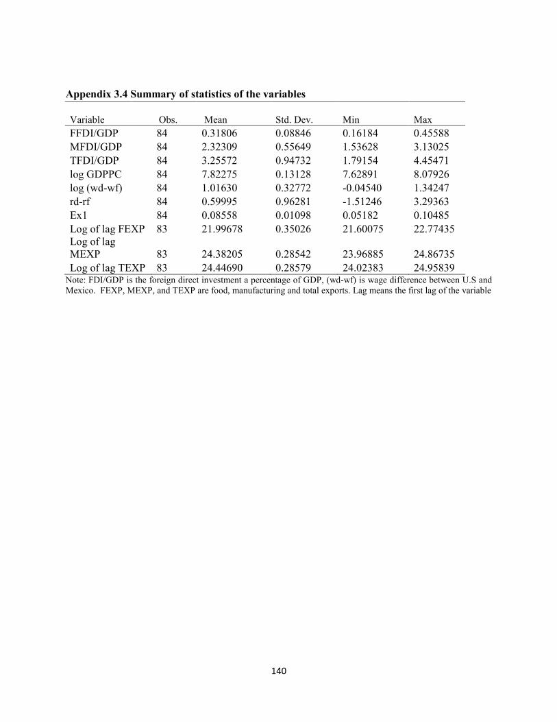
140

Appendix 3.4 Summary of statistics of the variables

Variable Obs. Mean Std. Dev. Min Max

FFDI/GDP 84 0.31806 0.08846 0.16184 0.45588

MFDI/GDP 84 2.32309 0.55649 1.53628 3.13025

TFDI/GDP 84 3.25572 0.94732 1.79154 4.45471

log GDPPC 84 7.82275 0.13128 7.62891 8.07926

log (wd-wf) 84 1.01630 0.32772 -0.04540 1.34247

rd-rf 84 0.59995 0.96281 -1.51246 3.29363

Ex1 84 0.08558 0.01098 0.05182 0.10485

Log of lag FEXP 83 21.99678 0.35026 21.60075 22.77435 Log of lag MEXP 83 24.38205 0.28542 23.96885 24.86735

Log of lag TEXP 83 24.44690 0.28579 24.02383 24.95839 Note: FDI/GDP is the foreign direct investment a percentage of GDP, (wd-wf) is wage difference between U.S and Mexico. FEXP, MEXP, and TEXP are food, manufacturing and total exports. Lag means the first lag of the variable

141

Appendix 4.1 Variable descriptions and source of data

Variable name Variable description Source

GDP Log of gross domestic product World Development Indicators

online version, World Bank 2011

Exports Log of real exports World Development Indicators


Imports Log of real imports World Development Indicators


FDI

Log of real foreign direct investment

which is calculated by deflating with

Mexican GDP deflator

GFCF Log of real gross fixed capital formation

LFT

Economically active population. Derived by

dividing the GDP of Mexico by GDP per

worker

Own calculation

GDP deflator Gross domestic product deflator International Financial Statistics

CD-ROM, IMF, 2010

GDP per

worker Gross domestic product per worker

Penn World Table 7.0, 2011

Note: all variables are in U.S dollars (2000)

142

Appendix 4.2 Summary Statistics of the Variables

Variable Obs Mean Std. Dev Min Max

Log of GDP 40 26.7171 0.3783901 25.92151 27.27588

Log of Exports 40 24.67728 1.11464 22.81193 26.25833

Log of Imports 40 24.87174 0.9240423 23.58061 26.38091

Log of FDI 40 22.32472 1.111539 20.20276 24.09562

Log of GFCF 40 25.0803 0.4193365 24.27473 25.83744

Log of LFT 40 17.10974 0.3742294 16.40425 17.66449

143

Appendix 4.3 List of the variables that are in each model

Model 1 GDP and Exports

Model2 GDP, Exports and Imports

Model 3 FDI and GDP

Model 4 FDI , GDP, and Exports

Model 5 FDI, GDP, Exports, and Imports

Model 6 FDI, GDP, Exports, Imports, GFCFF, LFT

144

Vita

Shanta Parajuli, daughter of Mr. Shiva Prasad Parajuli and Mrs. Radha Devi Parajuli was born in

Pokhara, Nepal. She graduated with a Master’s degree from the Tribhuvan University of Nepal

in 2000. In January, 2004 she entered graduate school at Alabama Agriculture and Mechanical

University, Alabama. In the fall of 2007, she was admitted to the doctoral program in the

department of Agricultural Economics and Agribusiness at Louisiana State University. She is

currently a candidate for the degree of Doctor of Philosophy, which will be awarded in May of

2012.

Documents

Examining the relationship between the exchange rate