Embed Size (px)
Citation preview

Examining the Impact of the East Asian Crisis on Household Savings in Indonesia
By Matthew R. Jones
Advised by Dr. Amyaz Moledina
Second Reader
Dr. Barbara Burnell
Submitted in Partial Fulfillment of the Requirements of the Senior Independent Study of the Department of Economics at the College of Wooster
March 2005

i
Acknowledgements
I would first like to thank my advisor Dr. Amyaz Moledina for providing
substantial motivation, support and time throughout the course of this project. I never left
the office without a sense of confidence (well, generally). I must also recognize Jing
Huang for helping with the mathematical derivations. Thanks also to Nathan Malcomb
for spending long hours in the editing process on the highway to and from the land of
Arizona. Thanks to my dear friend Roger Ekstrom for preparing a terrific stew on
Saturday. Finally, I wish to thank my dear and beloved friends and family for the good
times, without whom I would possess neither a complete thesis nor a sane mind.

ii
Abstract
This thesis analyzes the impact of the East Asian crisis on households in
Indonesia. It is predicted that the crisis would have slightly negative effects on
household savings. The results provide some evidence to this end, although the model as
a whole does not appear to be very robust. Furthermore, there is evidence in support of
both the precautionary savings motive of households and life cycle savings effects. Panel
data provided by the Indonesian Family Life Surveys of 1997 and 2000 from the Rand
Corporation were used to complete this analysis.

iii
Table of Contents
Abstract ......................................................................................................................... ii 1. Introduction .............................................................................................................. 1
1.2 A Brief History of the Indonesian Experience........................................................ 1 1.3 Introduction and Organization of the Paper............................................................ 3
2. Theory ....................................................................................................................... 6 2.1 Introduction........................................................................................................... 6 2.2 Life Cycle Model .................................................................................................. 7 2.3 The two period life cycle model formally derived................................................ 16 2.4 The Permanent Income Hypothesis...................................................................... 23 2.5 Precautionary Savings Model .............................................................................. 26 2.6 Applying the Standard Savings Model to the East Asian Crisis............................ 29 2.7 The Likely Effects of the East Asian Crisis on Savings........................................ 34
3. Review of Literature ............................................................................................... 37 3.1 Introduction......................................................................................................... 37 3.2 Literature Review One: “The Asian Crisis, Private Sector Saving, and Policy Implications” by Yun-Hwan Kim.............................................................................. 41 3.3 Literature Review Two: “Unemployment, Consumption Smoothing, and Precautionary Saving in Urban China” by Xin Meng................................................. 47 3.4 Literature Review Three: “Tests of the Permanent Income-Life Cycle Hypothesis Based on Household-Level Panel Data from Korea” by Michael D. Hurd and Hoe-Kyung Lee. ............................................................................................................... 57 3.5 Literature Review Four: “Risk, Natural Disasters, and Household Savings in a Life Cycle Model” by Mark Skidmore.............................................................................. 65 3.6 Literature Review Five: “The Household Response to the Mexican Peso Crisis” by David J Mckenzie...................................................................................................... 72 3.7 Literature Review 6: “Using Weather Variability to Estimate the Response of Savings to Transitory Income in Thailand” by Christina Paxson................................ 84
4. Model Specification................................................................................................. 93 4.1 Data .................................................................................................................... 93 4.2 Methodology: Conceptual Hypothesis ................................................................ 94 4.3 Methodology: Operational Hypothesis.............................................................. 100
5. Results ................................................................................................................... 107 5.1 Introduction....................................................................................................... 107 5.2 Results from the Pooled Sample Regressions..................................................... 107 5.3 Results from the Stratified Sample Regressions ................................................. 115 5.4 Aside: The Log-Dependent – Log-Independent Variable Model ........................ 121
6. Conclusion............................................................................................................. 124 6.1 Discussion......................................................................................................... 124 6.2 Final Conclusions.............................................................................................. 127 6.3 Suggestions for improving the model ................................................................ 129
Bibliography.............................................................................................................. 131 Appendix A: Regressions on Savings1a: Income – Expenditures – (Weekly Food
Expenditures)*52. ......................................................................................................... a

iv
Appendix B: Regressions on Savings5: Total Household Assets but not including educational expenditures. ............................................................................................. c Appendix C: Regression on Savings1 without Age3 ..................................................... e Appendix D: Summary Statistics of mover households and non-mover households. .f
Appendix E: Regressions Instrumenting HHincome rather than Quintile on Savings2 ......................................................................................................................... g
Appendix Ea: Regression Instrumenting HHincome rather than Quintile on Savings1 .......................................................................................................................... i Appendix F: Running Savings1 when Inschool is dropped.......................................... j
Appendix G: Results from a double log model running the log of Savings1 and the log of HHincome. .......................................................................................................... k Appendix H: Summary Statistics ................................................................................. l

1
1. Introduction
1.2 A Brief History of the Indonesian Experience Between 1970 and 1997 Indonesia proved to be one of the most successful
economies in the developing world: growth averaged a remarkable 7.2%, allowing real
incomes to increase four-fold during this period and dramatically reduce poverty rates
(Radelet 2000, 40).1 However, in July 1997, economic pressures forced Thailand to float
its currency, the baht. Investor panic ensued which caused the exchange rate to
overshoot, depreciating the currency more than was necessary (Flatter 2000, 71).1 The
panic made investors question the underlying economic stability of other East Asian
economies.
In the case of Indonesia, Radelet notes four underlying economic problems that
contributed to the crisis in Indonesia (Radelet 2000, 42-48). First, Indonesia’s relatively
high level of dependence on short-term borrowing from foreign investors made it
susceptible to quick withdrawals of capital during a panic. Second, financial market
liberalizations in previous years improved growth but regulatory mechanisms were not in
place to ensure stable and prudent banks. Third, the exchange rate was overvalued,
reducing export growth substantially. Finally, President Suharto’s family and friends
controlled significant business interests, which made them overly attractive to foreign
investors because of a perceived view that Suharto would protect these businesses.
Despite these underlying problems, Radelet notes that “Mismanagement of the
crisis by the Indonesian government, especially President Suharto, and by the
International Monetary Fund (IMF) made the contraction much deeper than was
1 Please see Chow and Gill (2000).

2
necessary or inevitable (Radelet 2000, 40). Despite some early warnings, the Indonesian
government ignored many of the economic weaknesses mentioned above for a significant
period of time. Moreover, as the downturn began, President Suharto’s continued favors
to his family’s businesses further undermined investor confidence (Radelet 2000, 59). In
response to the initial economic decline, the IMF recommended tightening fiscal and
monetary policy. However, lower government spending only worsened the economy.
Tighter monetary policy to raised interest rates but did not increase savings nor did it
reduce the upward pressure on the exchange rate. Furthermore, the higher interest rates
further decreased investment (Radelet 2000, 50). The IMF also recommended that banks
be closed in order to indicate that the government was serious about reform. However,
because there was no system of deposit insurance in place, bank runs followed (Radelet
2000, 51).
Political repercussions also followed the panic. Amid the crisis, Suharto
attempted to consolidate his power by replacing many of his economic managers with
“close associates and cronies” (Radelet 2000, 60). Student protests, rioting and incidence
of ethnic violence against Chinese ensued. In May 1998, President Suharto resigned and
left a political vacuum. Fortunately, by 1999 economic indicators began to improve: the
exchange rate and inflation fell, and interest rates began to decrease as well (Radelet
2000, 61).
Overall, in 1998 the crisis caused GDP to fall by 14% (Radelet 2000, 39).2
Poverty also increased relatively dramatically from 12.4% to 24.5% based on estimates
2 A side note that must be discussed is that the financial crisis also coincided with the effects of El
Niño, which caused a drought in the region. Datt and Hoogeveen (2003) find that the El Niño effect may have been more negative to household incomes than the financial crisis. Because of this side effect, we

3
by Skoufias et al (2000). Hence the immediate consequences of the Asian crisis were
quite harsh.
1.3 Introduction and Organization of the Paper
In light of the impacts of the East Asian crisis, this paper seeks to determine the
effects of the crisis on household savings in Indonesia. This shall be accomplished by
analyzing household savings shortly before and after the crisis occurred. The study of
savings is very relevant when evaluating the welfare of households. At its most basic
level, savings allow households to maintain a sufficient level of consumption in the event
of a negative shock. This use of savings becomes especially important in developing
countries where unemployment insurance and other social safety nets are uncommon.
Furthermore, at retirement a household consumes its savings when it no longer has a
stream of income. Hence, savings not only helps shield household welfare during a
crisis, but it will be of critical importance at retirement. For this reason, it is important to
determine if households will have a level of savings to buffer against future income
shocks.
Additionally, with regard to the overall economy, much of the rapid growth of the
East Asian economies has been attributed to high savings rates that led to capital
accumulation and thus growth.3 To the extent that the Asian crisis could affect the level
of savings, the crisis may have implications for the long run growth of the economy and
of household income in general.
shall refer to the events in East Asia not as the “East Asian financial crisis,” but simply as the “East Asian crisis.” 3 This argument is made by You (1998) and Young (1995) among others.

4
The rest of the paper will be organized as follows. Chapter 2 provides an
overview on the theories of saving behavior. First, what shall be the basis for our
analysis, the two-period life cycle model of savings, is examined in detail and then
formally derived. The permanent income hypothesis and the precautionary savings
model are then discussed. From the theory chapter, it is hypothesized that the effect of
the crisis on savings will be relatively small because the crisis is expected to have only a
temporary effect on income. Hence, the negative impact on savings should be relatively
small. Furthermore, increased income uncertainty may spark a precautionary motive,
causing risk-averse households to increase savings. Overall, it is expected that the crisis
may cause savings to fall slightly as a result of the crisis. Also, it is hypothesized that
savings among urban households may be relatively more negatively impacted than rural
households because the crisis may have concentrated its effects in urban areas.
In order to refine the view of issues surrounding the impacts of the Asian crisis on
savings, reviews of relevant literature are completed in Chapter 3. A number of
important conclusions are drawn from the literature. First, it is important to accurately
measure savings and income in order to get satisfactory results. Including durable goods
and educational expenditures might be important to the measurement of savings.
Education is an investment in human capital that provides returns in the form of higher
future income. Durable goods may be used as savings in the presence of imperfections in
financial markets. Certain demographic variables emerge as being of particular
consequence. In particular, the age of the household members has significant impacts on
the level of household savings. Also, the education level was found to have positive

5
impacts on savings as education increases, but households in higher educational cohorts
may be more affected by the crisis relative to lower educated cohorts.
Chapter 4 addresses the dataset and methodology that will be used to estimate
the impact of the crisis on household savings. Here, it is decided that two different
measures of savings will be used: the first measures savings out of income from the past
year while the second measures the total value of household assets, an aggregate measure
of savings. This is done in order to separate the effects of the crisis on the flow of
savings versus the stock of savings.
In Chapter 5, the results of empirical estimations are discussed. We find evidence
that the crisis did have negative impacts on household savings. In general, after the
crisis, total assets are found to be lower than before the crisis. Some evidence in support
of the precautionary savings model is found because, although assets are lower after the
crisis, households are found to be saving more out of current income than was the case
before the crisis. Relatively strong support is shown for the life cycle effects of savings.
Results show that households increase savings up to middle age and reduce savings
thereafter. There is also weaker evidence that supports the hypothesis that savings
increases as the education level of the household head increases.
Finally, Chapter 6 concludes with suggestions for future work as well policy
implications.

6
2. Theory
2.1 Introduction The East Asian financial crisis is likely to have caused significant changes in
household savings. Before we can theorize the effects of the crisis on savings, however,
it is necessary to first understand the most important savings models. In this chapter, the
most widely used theories explaining intertemporal consumption and savings are
discussed. The theories explored in this chapter relate to the individual, but they apply to
households as well. First, the life cycle model is examined and derived. Modigliani and
Brumberg first posited the life cycle model in 1954. It states that individuals wish to
maintain smooth consumption over their lifetime. Hence, consumption choices are based
on lifetime income. Next, the permanent income hypothesis by Friedman (1957) and
Hall (who added rational expectations to the model in 1978) will be discussed. The
permanent income hypothesis differentiates between permanent and transitory income,
making it a useful tool to analyze the ability to smooth consumption. It shall become
evident that the differences between the permanent income hypothesis and the life cycle
model are mainly in details that reflect how the models are used in empirical work. Then
the precautionary savings model is introduced. This model is often added to traditional
savings models in order to better explain consumer behavior under income uncertainty.
Its main conclusion is that under uncertainty regarding the future, individuals increase
savings to counteract negative shocks that might occur. Next, the standard intertemporal
savings model is applied to the East Asian crisis. Specifically, we show the effects of
permanent versus temporary changes in income. We conclude Chapter 1 by theorizing
that because the crisis caused only temporary drops in household income rather than

7
permanent drops, it is likely to have a slightly negative effect on savings, but that this
effect may vary across urban and rural households, who were impacted differentially by
the crisis.
2.2 Life Cycle Model The life cycle model states that the individual must determine how to allocate
consumption over his or her lifetime to best maximize utility. The most important
assumption the life cycle model makes is that the individual has a desire to maintain
relatively even consumption over his or her lifetime. Hence, the individual prefers to
smooth consumption in each period. Considering two periods, this idea of "consumption
smoothing" means that the individual tries to consume equal levels of consumption in
each period rather than a high level of consumption in one period and a low level of
consumption in the other.
A basic lifecycle model indicates that individuals allocate their consumption in
each period based on present income, future income and the real interest rate. Because of
the desire to smooth consumption, a change in one of these variables will alter
consumption choices in the present period and the subsequent period. In order to smooth
consumption, the individual may borrow or save to equalize consumption over his or her
lifetime. The individual makes allocation decisions between current and future
consumption based on the real interest rate. The model assumes that the interest rate at
which the individual can borrow and lend is the same. Hence there are no liquidity

8
constraints.4 The implications of this assumption will be discussed on page 14. If the
individual saves some of his or her income, then in the following period, the individual is
able to consume that savings in addition to the interest earned on the savings. Thus, the
real interest rate determines the relative price of future consumption versus current
consumption. The higher the real interest rate is, the higher the return to savings. A
higher real interest rate decreases the relative price of future consumption and increases
the relative price of current consumption. Therefore a high real interest makes future
consumption more attractive and current consumption less attractive. Conversely, a
lower real interest rate makes the relative price of future consumption more expensive;
this causes present consumption to become more attractive. Hence, changes in the
interest rate alter the relative price of future consumption and therefore savings decisions.
The specific effects of a change in the real interest rate are examined on page 11.
The budget constraint is represented in Figure 1 as the line AB; it provides all
possibilities to divide lifetime income between present and future consumption. The
individual maximizes utility somewhere along this line because it represents a complete
exhaustion of lifetime wealth. Consuming below the line is inefficient because it
indicates potential consumption not taken.5 The horizontal intercept at B is the maximum
income available that can be spent in the present period, that being y1+ )1(
2
r
y
+. Hence
the individual has available in the first period his or her first period income, y1, as well as
the discounted present value of future income )1(
2
r
y
+ (that would be borrowed). The
4 The term “liquidity constraint” refers to a case in which an individual is either unable to borrow as much as he or she desires or the interest rate at which the individual can borrow is greater than that at which he or she can save. Liquidity constraints are market imperfections resulting largely from imperfect information. 5 We assume there are no bequests, meaning the individual does not heir money to children, etc.

9
vertical intercept is the maximum amount of income that can be consumed in the future
period, y1(1+r) + y2. This is the value of present income plus interest earned at the real
interest rate, r, (meaning all first period income is saved) in addition to second period
income. The slope of the budget constraint is determined by the real interest rate, which
is the price of future consumption relative to current consumption. The slope is thus –
(1+r).
The endowment point is at E and represents the point where the individual does
not save or borrow but simply consumes first period income in the first period and second
period income in the second.6 If the individual is consuming on the budget constraint at a
point to the right of the endowment point, such as G, he or she is a borrower. At G, the
individual consumes more than first period income at c1G which is equal to first period
income plus the discounted value of the amount borrowed, x. To the left of the
endowment point, F for example, the individual is a lender. At F, the individual saves a
portion of first period income, z, to consume in the future. In the second period, second
period plus first period savings and interest can be consumed, y2+z(1+r).
6 E shall represent the endowment point in all future graphs.

10
Consider a change in current income on present and future consumption. If
current income increases, the budget constraint shifts out from BC1 to BC2 (see Figure 2).
If the individual consumes all of this increased income in the present period, he or she
will be at a point X on BC2; but X is not a utility maximizing point. Since the individual
has consumption smoothing tendencies, he or she increases consumption in the future as
well as in the present. Hence the individual saves some of this increased income to
consume in the future period. Therefore, the individual moves from a utility-maximizing
point at A to a new point at B, which reflects both increased current and future
consumption. If current income falls, then the individual consumes less in the present
period, but here the consumption smoothing principle causes the individual to reduce
savings or to borrow in the first period to offset the reduction in current consumption.
Borrowing money or reducing savings causes consumption in the second period to also
Present Consumption, C1
Future Consumption, C2
A
B
• Slope of AB = -(1+r) • A = y1(1+r) + y2 • B = y1+y2/(1+r) • c1
G =y1+x/(1+r) where x is the amount borrowed • c1
F = y2+z(1+r) where z is the amount saved
E
Figure 1: The Budget Constraint
G
F
y1=c1
E
y2=c2
c1G
E
x
E
x/(1+r)
E
y2-x
z
E
z(1+r)
E
c1F
y1-z
E

11
fall. Remember, the amount the individual saves or borrows depends on the real interest
rate.
The effects of a change in future income are similar. If future income falls, then
the individual will reduce current consumption. The reduction in current consumption
will be saved in order to offset the reduction in future consumption. An increase in future
income will cause the individual to increase future consumption. But the individual will
desire a higher current consumption as well. Hence the individual will reduce savings in
the current period, or borrow to increase current period consumption.
Since the real interest rate serves as the price of future consumption, a change in
the real interest rate also has an impact on intertemporal consumption and savings
decisions. The way in which these decisions are affected depends upon whether the
individual is a lender or a borrower. Let us consider the effects of changes in the real
interest rate for a lender. An increase in the real interest rate causes the relative price of
Present Consumption, C1
Future Consumption, C2
U1
U2
BC1
A
B
Slope of BC1 = Slope of BC2 = -(1+r) E represents the endowment point.
AC1
AC2
BC 1
BC2
X
Figure 2: An Increase in Current period consumption
U1 BC1
BC2 E1 E2 D

12
future consumption to decrease. In Figure 3, this effect is illustrated with a “rotation” of
the budget constraint where BC1 represents the initial budget constraint and BC2 is the
new budget constraint after the increase in the real interest rate. The budget constraint
rotates around the endowment point because the endowment point is not impacted by
changes in r. If all consumption occurred in a single period, the new budget constraint,
BC2, provides higher potential future consumption, but lower potential current
consumption. A change in r has two effects: a substitution effect and an income effect.
The higher real interest rate makes future consumption more attractive, causing the
individual to prefer more consumption in the future. Hence the individual substitutes
away from current consumption and towards saving, moving along U1 from A to X.
Ignoring for a moment the income effect, savings increases from A1E to X1E. The
substitution effect acts to reduce current consumption and increase future consumption.
A higher real interest rate also creates an income effect. Because the return on
saving is higher, an increase in the real interest rate causes the individual's wealth to rise
– the income effect. This increase in wealth occurs in the second period and is equivalent
to a rise in second period income. The wealth increase causes the individual to increase
consumption in both periods, and the individual reduces savings in the current period to
finance increased current consumption. Hence the income effect works to increase
current consumption but reduce savings. The move form X to B represents the income
effect.

13
Thus the income and substitution effects work in opposite directions for current
consumption and current savings; the total impact of these variables depends on which
effect is stronger. However, the income and substitution effects operate in the same
direction for future consumption, which will increase. In the example of Figure 3, the
individual moves from A to B and current consumption increases. Here the income
effect is dominant and savings falls from A1E to B1E.
Now a decrease in the real interest rate for a lender is examined. The relative
price of future consumption is now higher, which amounts to a decrease in wealth for the
lender. The income effect serves to decrease current and future consumption, and
decrease savings. The lower real interest rate causes the individual to substitute away
from savings and towards current consumption. Hence, the substitution effect will
decrease savings and future consumption and increase current consumption. The total
Present Consumption, C1
Future Consumption, C2
U1
U2
BC1 BC2
A
B
Slope of BC1 = -(1+r1) Slope of BC2 = -(1+r2) where r2 > r1
AC1
AC2
BC 1
BC2
Figure 3: The Effects of an Increase in the Real Interest Rate for a Lender
X
E B1 A1 X1

14
effects on current consumption depend on the strength of the respective income and
substitution effects, but future consumption and savings will fall.
A borrower behaves differently when the interest rate changes. A higher real
interest rate makes the relative price of current consumption higher than the relative price
of future consumption. Again, these affects are shown by rotating the budget constraint
around the endowment point in Figure 4 below. Since the individual will have to pay
back the loan in the second period, an increase in the interest rate causes lifetime wealth
to fall. The individual reduces future consumption to make up for the lost wealth.
Current period consumption also decreases and borrowing decreases (or the individual
begins to save) to offset the loss in wealth in the second period. These are the income
effects. The higher real interest rate causes the individual to substitute away from current
consumption at point A on U1 and towards less borrowing at point X. The substitution
effect decreases borrowing from E1A to E1X1. This serves to increase future
consumption. The income and substitution effects both work to decrease current period
consumption and decrease borrowing. Therefore the individual moves from point A on
U1 to point B on U2. However the income and substitution effects work in opposite
directions with regard to future consumption, so future consumption may increase or
decrease with a higher interest rate. In the case of Figure 4, future consumption increases
and borrowing falls from the initial level of E1A to E1B1.

15
A lower real interest rate will have positive wealth effects for a borrower. The
income and substitution effects increase current consumption and borrowing. The
individual will substitute towards current consumption by borrowing more, thereby
reducing future consumption. But the positive income effect reduces borrowing and
therefore future period consumption. Thus, the strength of the opposing income and
substitution effects will determine if future consumption rises or falls. In Figure 4,
imagine the effects of having an initial budget constraint at BC2 rather than BC1, then the
individual will move from point B to point A.
A significant assumption the life cycle model makes is that individuals face no
liquidity constraints: they are freely able to lend and borrow, and the interest rate at
which they are able to borrow is the same as the interest rate at which they can lend. In
reality, individuals are liquidity constrained, and this is particularly true in developing
countries (Deaton, 1991). Hence, the borrowing interest rate is higher than the lending
Present Consumption, C1
Future Consumption, C2
U1
U2 BC1 BC2
A
B
Slope of BC1 = -(1+r1) Slope of BC2 = -(1+r2) where r2 > r1
AC1
AC 2
BC1
BC2
Figure 4: The Effects of an Increase in the Real Interest Rate for a Borrower
X E
E1 B1 X1

16
interest rate. Furthermore, it is often much more difficult for lower income individuals
and households to receive loans. This can have a significant impact on the intertemporal
consumption-savings decisions of the individual.
For example, consider a reduction in current period income in the presence of
liquidity constraints. If the individual does not save a large portion of current income,
and income falls significantly, in order to smooth consumption, the individual will
borrow. If liquidity constraints do not allow the individual to borrow, the individual will
not be able to smooth consumption. Consequently, he or she will be forced only to
consume the income received in the current period. If the individual is able to borrow but
at a higher rate than the real interest rate on savings, this will also create inefficient
outcomes because the individual will not be able to borrow as much as he or she
otherwise would if the lending and borrowing rates were equal. Again, consumption
smoothing would be limited. The same principles apply to changes in the real interest
rates for borrowing or saving and future incomes. Generally, liquidity constraints limit
an individual's ability to smooth consumption. The next section will provide a formal
derivation of the life cycle model for two periods, in order to illustrate the consequences
of the model mathematically.
2.3 The two period life cycle model formally derived
Individuals maximize utility by allocating consumption smoothly over a lifetime.
The individual makes consumption and savings decisions for two periods, present and
future, whereby decisions regarding savings and consumption in the first period affect
decisions regarding consumption in the future period. The consumption and savings

17
decisions are influenced by the real interest rate, and changes in current and future
incomes. Now that intertemporal savings has been described conceptually, it is now
possible to formally derive the two period life cycle model.7
First we must derive the lifetime budget constraint:
c1 + s = y1 1.
This states that consumption in the first period, c1, plus savings in the first period, s, is
equal to first period income, y1. Solving for savings gives
s = y1 – c1 2.
In the second period, the individual consumes income from the second period as well as
the savings with interest from the first period. Hence,
c2 = y2 + (1+r)s 3.
Thus, savings is given by,
r
ycs
+
+=1
22 4.
Given income and consumption in both periods, we can construct the lifetime budget
constraint.
r
yy
r
cc
++=
++
11
2
1
2
1 5.
Solving for c2,
)1()1( 1212 rcyyrc +!++= 6.
These are relative values where r+1
1 is the opportunity cost of present consumption. Thus
the cost of one unit of present consumption is equal to 1+r units of future consumption.
7 The following is adapted from Williamson (2005).

18
Furthermore, the left-hand side of Equation 5 is lifetime consumption and the right side is
lifetime income. The individual will maximize utility subject to the budget constraint.
We assume that current consumption and future consumption are both normal goods and
that the individual has a desire for smooth consumption over each period. Therefore, we
maximize consumption over both periods, maxU[c1, c2].
In order to maximize the utility function above, we derive the LaGrangian:
L = [ ] !"
#$%
&
+''
+++
r
cc
r
yyccU
11, 2
1
2
121( 7.
Then, the derivative with respect to the first period terms, the second period terms, and
! , the LaGrangian multiplier, are given respectively,
!
U1c1,c2[ ] " # = 0 8.
!
U2c1,c2[ ] "
#
1+ r= 0 9.
!
y1+
y2
1+ r" c
1"c2
1+ r= 0 10.
Equation 8 gives the marginal utility of consumption in the first period minus ! ;
Equation 9 is the marginal utility of consumption in the second period, while Equation 10
is the budget constraint. The marginal utility of consumption is the amount of utility
attained from an extra unit of consumption in one period holding consumption in the
other period constant. Equations 8, 9 and 10 provide the first-order conditions necessary
to reach an optimum.
Next we eliminate ! by dividing Equation 8 by Equation 9:
[ ] !=+ )1(, 211 rccU 11.
Substituting gives: [ ] [ ] 0)1(,, 212211 =+! rccUccU 12.

19
Further modifying Equation 10 gives us:
0)1()1( 2121 =!+!++ crcyry 13.
Rewriting Equation 12 as [ ][ ]
)1(,
,
212
211r
ccU
ccU+= shows that the marginal rate of substitution
of current consumption for future consumption is equal to the interest that can be earned
on saving, that being one plus the real interest rate. Equations 12 and 13 allow us to find
the maximizing point of consumption and savings for the individual. In order to analyze
the effects of changes in present income, future income and real interest rates, it is
necessary to totally differentiate the two equations. Totally differentiating Equation 12:8
0])1([])1([
0)1()1(
22
'
22
'
121
'
1211
2222112212111
=!+!++!=
=!+!+!+=
drUdcUrUdcUrU
drUdcUrdcUrdcUdcU
14.
And totally differentiating Equation 13:
0)1()()1(
0)1()1(
211121
211211
=+++!+!+!=
=!!+!+++
dydyrdrcydcdcr
dcdrcdcrdydrydyr 15.
The equations can be written as matrices
!"
#$%
&
'+'''=!
"
#$%
&!"
#$%
&
'+'
+'+'
2111
2
2
122121211
)1()(1)1(
)1()1(
dydyrdrcy
drU
dc
dc
r
UrUUrU
Now, find the determinant:
22
2
1211
22121211
)1()1(2
)])1()(1[()]1)()1([(
UrUrU
UrUrUrU
+!++!="
+!++!+!=" 16.
8 A note on notation: U11 refers to the first derivative of the marginal utility of consumption in the first period, while U12 refers to the second derivative of the marginal utility of consumption in the first period. Hence, the first subscripted number refers to either the first or second period, and the second to the level of differentiation.
Matrix B Matrix A

20
To see the effects of a change in income on present and future consumption, we
differentiate Matrix B with respect to y and solve using Cramer’s rule:
!
+"+=
!
+"+=
])1()[1(
])1()[1(
1211
1
2
2212
1
1
UrUr
dy
dc
UrUr
dy
dc
17.
Here, 2212 )1( UrU +! represents future consumption and 1211 )1( UrU +! is
current consumption. Since they are both normal goods, they are both greater than zero,
2212 )1( UrU +! >0 and 1211 )1( UrU +! >0. Thus, 1
1
dy
dc>0 and
1
2
dy
dc>0. Hence, an increase
in income in the current period, dy1, will cause consumption to rise in both the current
(dc1) and future periods (2
dc ). This becomes more intuitive since the slope of 1
1
dy
dc and
1
2
dy
dc is positive. Hence, given an increase in an individual’s income in the first period,
the individual will use some of that income for present consumption. However, because
the individual wishes to have a smooth level of consumption over each period, he or she
will save some of the increased income, which causes consumption in the second period
to increase as well. This obviously shows that savings will also increase given the higher
first period income. This effect can be shown mathematically. Savings is given as
11cys != , differentiating with respect to current income illustrates the point made
above: =!=1
1
1
1dy
dc
dy
ds
!
++"'
12
'
11 )1( UrU>0 18.
In order to examine a change in future income, we now differentiate Matrix B
with respect to 2
dy and solve again using Cramer’s rule.

21
1
1
2
1
1
1
dy
dc
rdy
dc
+= >0 19a.
1
2
2
2
1
1
dy
dc
rdy
dc
+= >0 19b.
Therefore, we see again that an increase in income in the future period will increase
consumption in both the current period and the future period. This is because, given a
known increase in future income, the individual will have a desire to consume more in
the current period, hence he or she will decrease savings, or perhaps borrow to smooth
consumption over both periods. Conversely, a decrease in future income will cause
consumption in both periods to fall. The fall in future income will cause future
consumption to decrease. Realizing a future fall in income, the individual will save in the
present period in order to maintain a relatively constant level of consumption in the future
period. Differentiating savings with respect to future income gives 2
1
2dy
dc
dy
ds!= <0,
which shows that savings decreases when future income increases, and savings increases
when future income falls.
Finally, let us examine the consumption-savings choice given a change in the real
interest rate, r. Changing the real interest rate will effectively change the relative price of
current consumption. Again, we use Cramer’s rule, this time with the change in interest
rate, dr.
!
dc1
dr="U
2+ [U
12" (1+ r)U
22](y
1" c
1)
# 20.
!
dc2
dr=(1+ r)U
2" [U
11" (1+ r)U
12](y
1" c
1)
# 21.

22
The above equations include both income and substitution effects, hence we cannot
determine the sign of these equations. This result represents the income and substitution
effects that are involved in current and future consumption decisions given a change in
the real interest rate. If utility is held constant, the specific income and substitution
effects can be examined.
The substitution effect in terms of current consumption and future consumption are
respectively:
!
dc1
dr="U
2
# 22.
!
dc2
dr=(1+ r)U
2
" 23.
The income effects are the total effects of the change in interest rate minus the
substitution effects:
!
dc1
dr=[U
12" (1+ r)U
22](y
1" c
1)
# 24.
!
dc2
dr=U11" (1+ r)U
12](y
1" c
1)
# 25.
Thus the substitution effects show that if the interest rate increases, current
consumption will fall and future consumption will increase. Regarding a fall in interest
rates, current consumption increases and future consumption falls, reflecting the
relatively higher price of future consumption. Likewise, a higher interest rate increases
savings, whereas a lower interest rate decreases savings. The income effect changes
current and future consumption in different directions depending on whether the
individual is a saver (y1-c1>0) or a borrower (y1-c1<0). If the individual is a lender, then
an increase in the real interest rate will cause him or her to increase future consumption,

23
because the relative price of future consumption has gone down. However, because the
individual is a lender, a rise in the interest rate increases total wealth, hence current
consumption may increase (and savings may decrease) if the income effects outweigh the
substitution effects. If the individual is a borrower, then as the interest rate rises, it
becomes more costly to consume in the current period. Hence the individual will reduce
current consumption and increase savings. Because future consumption will increase
given the substitution effect, but decrease due to a negative income effect, future
consumption depends on the strength of these diverging forces. Deriving the savings
function, s=y1-c1, with respect to r gives: dr
dc
dr
ds1!= . Changes in savings depend on
how consumption reacts to the change in the real interest rate and whether the individual
is a lender or a borrower.
2.4 The Permanent Income Hypothesis When the permanent income hypothesis and life cycle savings model were first
derived, they exhibited some differences. However, as the theories were refined over the
years, they have evolved to become close substitutes for one another. Both models state
that individual consumption choices are based on a lifetime annuity of resources and both
rely on the fundamental assumption that individuals prefer to smooth consumption
(Modigliani, 1986). Hence, the difference between the models essentially lies in
subtleties. The permanent income hypothesis is used primarily to test an individual’s
ability to smooth consumption. To do this, the permanent income hypothesis divides
income between “permanent income” and “transitory income.” Briefly, the standard
theory of savings will be discussed from the perspective of the permanent income

24
hypothesis. It will be seen that the overall themes from the life cycle model discussed
above remain the same.
Friedman defines permanent income as the annuity of the present value of
resources in addition to the discounted present value of all future resources (Friedman,
1957). Stated simply, permanent income is the average value per period of an
individual’s total lifetime net worth. Since the individual desires a smooth level of
consumption over time, he or she will consume a constant proportion of permanent
income.
Transitory income is the deviation of received income from expected income.
Transitory income is saved or dissaved in order to maintain the desired level of
consumption. Hence, if transitory income is positive, or greater than permanent income
for the specified period, that surplus will be saved. If transitory income is negative, then
the individual withdraws previous savings in order to maintain the same level of
consumption. An important conclusion is that transitory income is equal to the savings
for that period. Furthermore, very little of the transitory income is consumed. For
example, if transitory income equals $100, then the individual will save most of this
increase. The individual will spread out the consumption of the $100 over the rest of his
or her expected lifetime. If the individual expects to live for 9 more periods, then he or
she may consume $10 of the transitory income in the present period and save the rest. An
important property of transitory income is that it is unpredictable. Transitory income, by
definition of being the difference between received income and expected income
presumes unpredictability. This fact becomes critical in empirical testing because

25
measurements of transitory income must be completely exogenous from permanent
income and unpredictable.
The level of consumption will only change if the level of permanent income
changes. Thus, if permanent income increases, consumption will increase. Hall (1978)
concluded that if individuals have rational expectations then consumption increases by an
equal amount to the increase in permanent income. A change in an individual’s level of
consumption indicates that the individual has acquired new knowledge regarding his or
her permanent income. Thus, a change in permanent income is known as an “income
innovation” thereby reflecting new knowledge gained by the individual.
With positive transitory income, the individual increases savings by an amount
equal to transitory income.9 In the case of negative transitory income, received income is
lower than permanent income, causing the individual to withdraw savings. In both cases,
consumption will remain the same. However, consider a person who becomes disabled
and can no longer work. Now negative transitory income outweighs an individual’s
reserve of savings and he or she is unable to maintain the same level of consumption.
Given the new (but unfortunate) knowledge, the individual adjusts his or her expectations
regarding permanent income and therefore lowers consumption. Hence the permanent
income hypothesis still holds.
However, it is possible that, if the individual has no savings at all, then he or she
will be forced to consume transitory income even under a temporary shock that does not
affect permanent income. Hence, changes in transitory income may cause changes in
9 The permanent income hypothesis assumes individuals live for infinite periods. Hence, given an increase in transitory income, the individual will spread this income over infinite periods and an insignificant amount, nearly zero, will be consumed presently. Hence, the previous statement is not contradictory to the example presented on page 23 where we assumed an individual lives for 10 periods.

26
consumption. This occurs under liquidity constraints because the individual cannot
borrow in order to maintain the same level of consumption.
An income innovation that raises permanent income will show a corresponding
and equal increase in consumption. Finally, an increase in the real interest rate will cause
permanent income to increase because savings will earn a higher rate of return, thereby
increasing lifetime wealth. This increase in permanent income will cause consumption to
increase by an equal amount. A lower real interest rate will provide a negative income
innovation, lowering permanent income and decreasing savings and consumption.
The permanent income hypothesis is a better model to analyze consumption
smoothing because it divides income into transitory and permanent components.
Consider the examination of consumption smoothing in a typical life cycle model. If an
individual adjusts his or her expected lifetime annuity of resources (permanent income),
he or she will adjust consumption accordingly. As mentioned earlier, if the individual
becomes disabled, he or she revises lifetime expected income to a lower level (this
revision is known as an income innovation), and hence reduces consumption. Under a
life cycle model, this reduced consumption will falsely indicate an inability to smooth
consumption. However, the permanent income hypothesis notices that the change in
income is a permanent one, hence, the adjustment in consumption indicates consumption
smoothing still exists, but at a different level (DeJuan, 2003).
2.5 Precautionary Savings Model The precautionary savings model was developed in part to reconcile differences
between predicted savings behavior and actual outcomes. Traditional savings models

27
such as the life cycle and permanent income models predict that the level of consumption
should remain independent of income. Therefore consumption will remain smooth from
period to period even if income fluctuates. However, a considerable body of empirical
work has shown that consumption often follows a path that closely mimics income,
thereby questioning the validity of standard savings models.
The precautionary savings model offers a framework that explains the different
outcomes seen from standard models. Despite its relatively recent emergence, the
precautionary savings model’s theoretical foundation goes back to Keynes (1936), who
noted that one reason individuals save is “to build up a reserve against unforeseen
contingencies” (Browning and Lusardi, 1996). This section will provide an overview of
the precautionary savings model and its relevance to savings theory.
The basic assumption behind the precautionary saving model is that individuals
are prudent and also face a degree of uncertainty regarding future income. Because
individuals are uncertain about future income, they increase their savings in order to have
a supply of savings to guard against a negative shock. The greater the uncertainty, the
greater is the marginal propensity to save. The precautionary savings utility function can
be expressed thusly: U[C] = A
CA
!
!
1
1
, where C is consumption and A is the coefficient for
relative risk aversion (Zeldes, 1989). Hence the utility derived from consumption
depends on the level of uncertainty faced by an individual. This utility function differs
from that analyzed in the life cycle model described above because it is not simply
quadratic, but rather the individual has a “standard constant relative risk aversion”
(CRRA) utility function. When the individual displays a CRRA utility function, he or
she will consume less if wealth (i.e. savings) is low. Conversely, individuals with a

28
standard quadratic utility function will consume according to lifetime income, the level of
savings accumulated is of no concern (Zeldes 1989).
Much of the empirical literature has found that, counter to the traditional saving
theory, the consumption path closely follows the income path. The precautionary savings
model explains this result because increases in transitory income reduce uncertainty,
therefore a larger proportion of transitory income is consumed than traditional models
predict.
An extension of the precautionary savings model is the buffer-stock theory of
saving created largely by Christopher Carroll (1992). Carroll adds that individuals are
not only prudent, which provides the precautionary motive, but also impatient, causing
them to wish to consume, or draw down assets in the present (Carroll, 2). The impatience
criterion implies the existence of a “target wealth to permanent income ratio” (Carroll, 2).
When wealth (savings) is above the target ratio, the individual is dominated by
impatience and reduces savings or dissaves. If wealth is below the target, the
precautionary motive outweighs impatience and the individual increases savings. This
model is still very similar to the standard precautionary savings model. If uncertainty
about future income increases the target level of wealth, the desired stock of savings used
to buffer drops in income, increases and the individual saves more. The buffer-stock
model explains the parallel income and consumption paths noted empirically as a result
of individuals’ “impatience and their prudent unwillingness to borrow (Carroll, 3). Here
if income falls, uncertainty increases and the individual increases savings due to the
precautionary motive, and therefore reducing consumption. If income increases, the
individual becomes impatient and increases consumption, therefore reducing savings.

29
2.6 Applying the Standard Savings Model to the East Asian Crisis Given an understanding of the basic models used to describe the savings behavior
of individuals, it is now possible to apply these models to households’ experience of the
East Asian crisis. The crisis caused significant drops in household incomes. As was seen
above, a drop in income in either period will cause drops in consumption in both periods.
The overall impact on saving when comparing a period before the onset of the crisis and
a period after the crisis had ended will depend on whether the drop in income was
temporary or permanent. If the crisis caused incomes to fall only temporarily, meaning
that household income recovered after the end of the crisis, then the effect on the savings
rate should be relatively small but negative. Figure 5 represents the effects of the crisis
depending on whether it caused temporary or permanent changes in income. A
temporary change in income causes the lifetime wealth to be slightly lower, which is
reflected in the shift of the budget constraint from BC1 to BCT. Thus, the household
reduces both current and future consumption slightly, moving from point A to point B,
and therefore savings falls marginally from A1E to B1E1. If incomes remained
permanently lower as a result of the crisis, then the impact on savings would be much
more significantly negative, hence the shift in the budget constraint is much larger,
moving from BC1 to BCP. This shift reflects a much lower lifetime wealth, since income
in all future periods is expected to be less. The effect on consumption is much greater.
Households now maximize utility at point D, thus reflecting much lower consumption in
both periods than would otherwise be the case if the income effects of the crisis were
only temporary. A permanent income drop reduces savings more dramatically than a

30
temporary drop. In this case, a permanent income drop causes savings to fall to D1A1.
This line represents a much lower level of savings than if the income drop is temporary
and savings is B1E1.
In addition to causing incomes to fall, the crisis also had significant consequences
for the real interest rate as countries reacted to the crisis by using monetary policy. We
shall now examine the impacts of temporary and permanent income changes with the
inclusion of changes in the real interest rate.
If households experience both a drop in income and a change in the real interest
rate, then the affect of the crisis on household savings becomes more complex. First
consider an outcome where the crisis causes the real interest rate to rise. If a household is
initially a lender, then as we have stated previously, a fall in temporary or permanent
income will have the effect of reducing consumption in both periods as well as reducing
savings. Graphically, this is represented in Figure 6 as a move from point A on
U1
UP
A
B
UT
Future Consumption, C2
Present Consumption, C1
1PC P
tempC P
permC
D
1FC
F
permC
F
tempC
BCT BC1 BCP
Figure 5: The effects of Temporary and Permanent changes to income. Assume no changes in real interest rate. Initial savings: A1E Savings after a temporary drop in income: B1E1. A1E > B1E1 Savings after a permanent drop in
income: D1A1. B1E1 > D1A1
E A1
E1
B1 D1

31
indifference curve U1 to C on indifference curve UT. Savings falls from the initial
amount A1E to C1E1 after the income drop. The higher real interest rate rotates the
budget constraint BCT to BCT2. If after the temporary drop in income the household
remains lender (as is the case in Figure 6), then a higher real interest rate will prompt the
household to increase future consumption, moving back up to 2r
TU . The income effect
reduces savings and increases present consumption while the substitution effect works in
the opposite direction, increasing savings and lowering present consumption. Overall,
although the drop in income has negative effects on consumption and savings, the higher
interest rate is beneficial to a lender and hence, some of these negative effects may be
partially counteracted. Therefore, even though the household will still be worse off than
during the pre-crisis period, there may theoretically be an increase in savings, future
consumption, or even perhaps current period consumption.10 In Figure 6, when the real
interest rate increases, future consumption increases from an initial point of 1FC to
2Fr
TempC and current period consumption falls. Savings also increases from its value after
the income drop, from A1E1 to B1E1.
If the Asian crisis caused permanent drops in income, but the individual remained
a lender, the results would be the same as those mentioned above. However it could be
the case where the loss in income is so great that the individual is forced to become a
borrower; that is the individual now maximizes utility at a point below the endowment
line. This possibility is represented by the indifference curve UP. In this case, a higher
interest rate will not help the household, and utility would drop to 2r
PU . Given a drop in
10 If the increase in the real interest rate is large enough, it is technically possible, but unlikely, that the household becomes better off than it was initially, even considering the temporary drop in income.

32
permanent income that forces the household to borrow, it is quite unlikely that future
consumption or current consumption would increase as a result of the crisis, and
naturally, the household is made to borrow, so savings becomes negative.
Now assume the Asian crisis caused interest rates to fall. In this circumstance a
borrowing household will be examined regarding temporary and permanent losses in
income. If the household is initially consuming at the pre-crisis level, point A in Figure
7, and the crisis causes a temporary drop in income, the household will reduce savings
and consumption in both periods, therefore moving from A to C. However, a lower real
interest rate will lessen the impact of the crisis, allowing the household to borrow more,
increasing current consumption and reducing savings and future consumption. This
places the household at B on the indifference curve 2r
TU . If the change in income were
permanent the household would reduce savings and consumption to a much greater

33
degree, moving from A to E. Again, a lower real interest rate will dampen the negative
effects of the crisis for a borrower and the household will maximize utility at D. Notice
this represents even lower future consumption, and therefore more borrowing, than does
point E.
Hence, it can be seen that if the real interest rate falls during the crisis, then
household borrowing will increase as a result. Similarly, for lending households, savings
will fall. Notice however, that because the crisis caused bank failures in Indonesia, as
well as much greater precaution on the part of the lenders, it is likely that households
faced significant liquidity constraints during the crisis. Hence, households may not have
been able to increase their borrowing in the event of falling interest rates. Assuming
absolute liquidity constraints and no savings, households would not be able to reduce

34
future consumption below 1FC . Thus the household would be forced to consume at
inefficient positions on its budget constraint, such as BL and DL.
2.7 The Likely Effects of the East Asian Crisis on Savings The East Asian financial crisis is likely to have affected household savings in
conflicting ways. While falling incomes would clearly reduce household savings,
increased income uncertainty would encourage saving through the precautionary motive.
To theorize about the crisis’ total effect on household savings, let us first consider
whether the crisis had a temporary or permanently negative impact on income.
It seems likely that the crisis would cause household income to only temporarily
fall. GDP per capita statistics show that for most of the crisis-affected countries, incomes
dropped significantly in 1998 but began to rebound in 1999 (World Bank, 2004). GDP
per capita had fully recovered in the Philippines and even in Indonesia, the hardest hit
economy during the crisis, by 2000. Thailand, who was also highly affected, lagged
behind, but by 2002 GDP per capita was within a half percent of the 1996 level. Hence
the GDP figures do not show evidence of permanent drops in income, although some
economies rebounded more quickly than others. If we assume that the lower incomes
received by households as a result of the crisis were temporary, then the effect on
household savings should be relatively small and negative. However, although incomes
have rebounded from the crisis, GDP growth is now much lower relative to pre-crisis
statistics. GDP growth in Indonesia and Thailand was between 7 and 11% up to 1996.
After the crisis, growth has been much more modest, generally less than 5%. This

35
indicates that the growth rate of savings is also likely to be lower after the crisis, ceteris
paribus.
In Indonesia, interest rates increased during the crisis the government
implemented tighter monetary policy. Interest rates in Indonesia both before and after
the crisis followed no observable pattern. The effect of interest rates on savings is
theoretically ambiguous due to the substitution and income effects involved; hence, no
prediction is made as to the effects of the real interest rate on household saving behavior.
Before the onset of the crisis, the countries of East Asia enjoyed consistently high
growth and relatively low unemployment. The East Asian crisis severely impacted
incomes and caused higher unemployment and poverty rates (Kim, 340). In Indonesia,
the loss of control over monetary policy caused inflation to soar and some banks were
forced to close. Additionally, the crisis precipitated a change of leadership from the long-
standing Suharto regime. Hence, it is obvious that the Asian crisis would cause relatively
large increases in income uncertainty, especially in Indonesia. Uncertainty sparks the
precautionary motive, prompting households to save more. Since many households
probably viewed the pre-crisis economy as almost foolproof, the reality of the crisis
undoubtedly had a negative effect on the confidence of households.
Kim raises another issue of confidence that is important to the saving behavior of
households: the confidence in financial institutions. Kim notes that, “Before the crisis,
banking institutions in these economies had long enjoyed a high, probably perfect, degree
of confidence based on the belief that a bank was not prone to bankruptcy at all…” (Kim,
342). The crisis forced many banks to close in Thailand and Indonesia. The erosion in

36
confidence that would likely follow would cause households to move savings away from
banks and towards other savings instruments such durable goods or other assets.
Finally, the Asian crisis may have affected savings in a differential manner
between rural and urban households. Bresciani et al. (2002) state that urban areas bore
the brunt of the crisis, while the currency depreciation in Indonesia and Thailand may
have made some rural households better off because of improved export opportunities for
agricultural goods. Thus, the impact on savings between households in urban and rural
areas may be different. Urban areas may experience larger decreases in savings, while
urban areas might see only small differences, and perhaps even increased savings.
Overall, the impact on household savings is likely to be relatively small, both because the
fall in incomes is only temporary and because of the counteracting nature that the
precautionary motive provides.

37
3. Review of Literature
3.1 Introduction In this section, methodological and operational issues relevant to the examination
of household savings and to the East Asian crisis are culled from the literature. There are
a few common themes that emerge from the subsequent articles. First, it is evident that
the method of measuring income, consumption and savings can have a dramatic affect on
the results of an empirical estimation. This is especially true when testing the permanent
income hypothesis. The permanent income hypothesis is best used to analyze
households’ ability to smooth consumption and requires that income be separated into
transitory and permanent components. From theory, we know that the effect of
permanent income on savings should be close to zero while transitory income should
account for nearly all savings. To test the hypothesis empirically, it is necessary to obtain
a measure for at least one of these variables.
Unfortunately, it is difficult to find appropriate measures of permanent and
transitory income because of issues of endogeneity between the two variables. For
example, a measure of permanent income must not be affected by temporary shocks to
income. Likewise, a measure of transitory income must be totally unpredictable and
outside the control of the household. Meng (2003) estimates permanent income using a
weighted average of past incomes, whereas Hurd and Lee (1997) try to eliminate the
effects of transitory income by aggregating income and averaging it over the population
to reduce its influence (Hurd and Lee, 107). As it will be found, the technique of Hurd
and Lee might be less than desirable whereas Meng’s technique does not account for
future income expectations. Paxson obtains a measurement of transitory farm income

38
using deviations in rainfall. This method provided a new venue in the estimation of the
permanent income hypothesis, although it too has some flaws.
While choosing the proper estimation of permanent and transitory income is very
important, the permanent income hypothesis is best used to analyze households’ abilities
to smooth consumption. If a simple analysis of the change in saving is required, issues of
permanent and transitory income are less important. However, the ways in which
consumption, income and savings are measured may still have significant influence on
the results obtained. For example, Paxson notes that households tend to underreport their
income (perhaps to evade taxes or because some income was derived in black markets).
This underreporting will cause expenditures relative to income to appear to be higher
than otherwise and hence savings will appear lower than it is in actuality. Also, some
types of expenditures could be considered a form of savings. For example, expenditures
on education might be considered a form of savings if the human capital produced yields
higher incomes or the income of the individual who received the education is transferred
back to the individuals who paid for the education. Expenditures on durable goods might
also be a form of savings because durable goods yield a service over a longer lifespan
than a nondurable good. Therefore, durable goods may represent an investment. Paxson
takes this approach by including durable goods in her measurement of savings. Hence
when creating savings variables, it is important to consider the variety of measures that
could be afforded dependant upon what is included in the measure.
From the literature we find the importance of certain demographic variables in
their relation to savings. Educational expenditures as well as the general level of
education obtained by the household appear both in Mckenzie and Meng, who examine

39
educational expenditures during negative income shocks. Educational expenditure is an
important variable for two reasons. First, it relates to human capital development. If a
household is unable to smooth consumption of educational expenditures, there may be
serious long run implications for human capital development in the household and for
future incomes. Second, as alluded to earlier, expenditures on education may be a form
of savings. Investments in education will yield a long run return in the form of higher
income. If a household believes this return will be transferred back, i.e. if the parents
expect their children to care for them in old age, they have an incentive to spend on
education in the present in expectation of gaining some return to that investment in the
future. Interestingly, Meng and Mckenzie find divergent results when examining
educational expenditures during negative shocks. Meng finds that uncertainty decreases
expenditures on education, while Mckenzie finds that during the Mexican peso crisis
educational expenditures actually increased. These findings will be further discussed in
their respective reviews.
Other important demographic variables are shown to be the age of the household
members as well as the number of dependents in the household. It will be seen that
saving behavior varies with age, with saving being highest at middle age and lower at old
age and youth. The effects of age are important in providing support for the life cycle
model. Furthermore, a household with a large number of dependents (non-income
earners) are likely to depress saving since expenditures are required for the care of these
individuals. Households with members in school are also predicted to have lower savings
rates, but as mentioned above, expenditures on education could actually be a form of
savings.

40
The precautionary savings model appears in the articles by Meng, Skidmore,
Hurd and Lee, and Kim. This model states that households will increase saving under
uncertainty in order to guard against future negative shocks. Again however, the problem
arises in finding an appropriate measure of uncertainty. Skidmore is apparently
successful in measuring uncertainty by calculating uncertainty based on damages caused
by natural disasters over time (assuming that higher damages create higher uncertainty).
Meng is also successful in using a calculated likelihood of unemployment, although this
method may only be applicable to China, which had until recently guaranteed the
employment of its citizens. Hurd and Lee show that risk aversion and impatience plays a
role in determining the rate of savings. Kim predicts that the increased market volatility
from the Asian crisis will increase savings to some extent but drops in income will offset
this increase.
Finally, the issue of liquidity constraints naturally arises, since a household's
ability to smooth consumption may often depend upon its ability to borrow money if
savings is not sufficient. Hurd and Lee make specific attempts to test for liquidity
constraints. They find that liquidity constraints do impede consumption smoothing
abilities, but their measure is also somewhat of a compromise because it includes only
financial market constraints, but does not consider a household's ability to use assets to
smooth consumption. In the other articles the liquidity constraint problem is most
evident in cases where consumption smoothing does not occur. The rest of this chapter
shall discuss these points in more detail.

41
3.2 Literature Review One: “The Asian Crisis, Private Sector Saving, and Policy Implications” by Yun-Hwan Kim. “The Asian Crisis, Private Sector Saving, and Policy Implications” by Yun-Hwan
Kim provides a theoretical framework for analyzing the effects of the Asian Financial
Crisis on savings. Specifically, Kim evaluates the impacts of the crisis on private sector
savings both at the firm and household level in both the short and long run. Kim analyzes
savings from a relatively limited scope, focusing primarily on bank savings.
Furthermore, the author examines potential factors that have an impact on the savings
rate, including crisis-specific variables. A potential empirical model is presented,
although no empirical work is done. Given theoretical results, the author concludes with
policy recommendations. This review will focus most specifically on areas relevant to
household savings during the crisis.
Theory
Kim begins with an overview of the most prevalent theories on intertemporal
saving. The life-cycle model, of Modigliani and Brumberg (1954) is the standard
approach, stating that individuals wish to consume a relatively constant amount during
their productive and retirement years. Individuals save during their time employed and
then consume their savings at retirement. Since individuals have a desire to maintain a
relatively consistent level of consumption, a change or disruption in income will change
an individual’s rate of savings, resulting in consumption smoothing.
The precautionary savings model states economic uncertainty spurs the desire for
increased savings for the next period. A more specific model of precautionary savings,
Carroll’s buffer-stock model (1992), is concerned with the possibility of future
unemployment. Here, savings is regarded as the primary means to safe guard, or buffer,

42
consumption in the event of a spell of unemployment. As the risk of unemployment
increases, so does the level of savings.
Next Kim examines some theoretical factors that are important in determining the
level of savings within developing countries. In this section, the discussion of
demographic factors is of particular interest for examining household-level savings. Kim
paid particular attention to demographic variables cited in the work of Lall (1990) and
Burney and Khan (1992). Lall examined households in India while Burney and Khan
looked at households in Pakistan.
The key demographic factors Kim notes as being relevant to the Asian crisis are
briefly highlighted: Female heads of households tend to save more. Perhaps there is a
maternal instinct in women that promotes saving, or perhaps women are more risk averse,
therefore they save as a precaution. Further, if women are the primary caregivers, they
may have a tendency to save for their children. The dependency ratio is equal to the
number of dependents in a household relative to household size. It is found that as the
dependency ratio increases, savings falls, since dependent members contribute to
consumption but not income. It is found that the age of the household head affects
savings; as age of the head increases past middle age, savings decreases at a decreasing
rate, following the lifecycle theory. Individuals who are illiterate were found to save less,
perhaps because many savings plans are overly complex and involve excessive
paperwork (Kim, 336). Oddly, in the Pakistan survey it was found that as the education
of the household head increases, savings decreases. The justification here is that an
educated household head is more likely to have other members of the family pursue

43
higher levels of education, thereby increasing education expenditures and reducing
income.
Kim then moves on to other factors that might influence saving after the Asian
crisis. Because of the crisis, financial institutions are thought to have become more
cautious in making large loans to industry, hindering productive activity and therefore
raising the likelihood of unemployment at the household level (Kim, 346). Kim predicts
that financial market liberalization will have a negative short run impact on savings. He
asserts that financial market liberalization will lower the liquidity constraints faced by
households and hence increase borrowing. However, as is seen from above, financial
institutions might be less willing to lend. Even considering the liberalizations, it is likely
that households faced increasing liquidity constraints as a result of the crisis, making it
more difficult for them to borrow. Thus, Kim’s hypothesis may be false. In the very
long run, market liberalization should increase incomes and thus savings should increase
as well.
Leading up to the crisis, Asian countries enjoyed very stable economies. Kim
argues that the Asian crisis had a very large impact on economic uncertainty, which
reduced long run savings. One factor related to lower long-term savings is the
diminished confidence in financial institutions after the crisis since individuals will
decrease their savings if they do not trust the banks to keep their money safe. Kim
provides some evidence for this idea by examining changes in the allocation of different
time deposit maturities in Korea. In 1996, before the crisis, one-year deposit maturities
accounted for 17.1% of the market for deposit maturities while deposit maturities lasting
more than two years accounted for 39.2% of the market. After the crisis in 1999, these

44
deposit maturities reversed, accounting for 45.8% and 6.3% for the respective one-year
and over two year maturity rates. Unfortunately, we are unable to determine if the
number of deposits changed from his measure. Hence, although quite unlikely, the
changes above could occur if households were increasing the number of deposits in banks
and simply preferring short-term deposits to long term deposits. Thus, the evidence that
Kim provides for an erosion of long run savings is somewhat questionable.
Finally, increases in poverty should have a negative effect on savings. Kim notes
that increased poverty results in lower incomes, “difficulties planning long-term
consumption/savings options and results in poorer education of children, which has long-
term adverse implications for employment and income (Kim, 342). The poverty rate may
be a form of transitory income since Skoufias et al note that with respect to the impacts
of the crisis, “transitions into and out of poverty reveal remarkable fluidity” (Skoufias et
al 2000, 110). However, a methodological problem exists with this measure because
different measures of poverty may yield very different results.
Although, Kim does not conduct any empirical testing of his hypothesis, he does
provide some theoretical ideas about the effects of the Asian Crisis on savings. Kim
predicts a short run increase in savings during the crisis due to precautionary saving.
However, this increase will differ among households of varying incomes. Lower-middle
and middle income households will increase savings to create a larger reserve of savings
in light of higher unemployment risk. However, high income households will already
have significant savings, and hence they may not change their savings pattern much.
Kim theorizes that very poor households do not save a large amount to begin with and
they will therefore be unlikely to alter their level of savings significantly. However, as we

45
will see, Meng finds that most urban Chinese households were able to smooth
consumption even under unemployment, indicating an ability to alter savings (Meng,
483).
Kim believes that the long-run effects on savings will be negative due to the
decreased confidence in financial institutions, higher poverty rates, and “increased
variability in business sales” (Kim, 347). He also presents a number of policy
recommendations aimed at increasing long term savings plans. He suggests governments
should offer bonds in smaller denominations, create a system of deposit insurance,
increase levels of microfinance to increase savings in the informal sector where interest
rates are very high, and promote education, particularly of women in order to increase
future earning potential (Kim, 347-348).
Although Kim does not do any empirical analysis, he provides a potential
empirical model analyzing savings during the crisis. The model is based on the standard
household savings model: Sh = g(Y, R), which when incorporating the factors mentioned
above, is,
Sh = g(Y, R, v, p, c, f). 26.
Where Y is disposable income, R is the rate of return on deposits, v represents economic
uncertainty, p is the level of poverty, c represents confidence in financial institutions, and
f is financial liberalization. The author should also have included variables for the
demographic factors he mentioned earlier, but he neglected to do so. Kim has yet to test
the model because the recovery was not yet complete at the time of publishing. It is
expected that an increase in Y will cause savings to increase, changes in R are ambiguous.
Economic uncertainty, v, is expected to have a positive impact through the precautionary

46
savings motive, increases in poverty, p, are predicted to lower savings. Lower
confidence in banking institutions, c, should decrease bank savings and financial market
liberalization, f, is expected to negatively impact savings.
This article is particularly interesting because it relates exactly with what we wish
to analyze: the effects of the Asian crisis on savings. Although Kim’s proposed model
specifically pertains to the financial crisis, the relevance of financial market liberalization
is questionable. Kim predicts financial market liberalization to have a negative impact on
savings. However, as mentioned above, the effects of financial market liberalization
during the crisis may be limited because liquidity constraints are likely to have increased
during the crisis regardless of liberalizing efforts. Measures of economic uncertainty and
confidence in financial institutions both relate to precautionary savings, with economic
uncertainty determining the level of precautionary saving and confidence in banks
determining the method of saving chosen (such as assets or savings accounts). These
variables may be of great importance over the financial crisis. Yet they may also be quite
difficult to quantify. Overall, Kim’s framework includes some very relevant variables
relating to the Asian financial crisis, but also some that may not be particularly relevant.

47
3.3 Literature Review Two: “Unemployment, Consumption Smoothing, and Precautionary Saving in Urban China” by Xin Meng.
Xin Meng’s article “Unemployment, Consumption Smoothing, and Precautionary
Saving in Urban China” provides insight into how urban households in China are able to
react to dramatic increases in uncertainty and the frequency of income shocks. In the
mid-1990s, China underwent significant economic reforms that greatly liberalized much
of the economy. Small and medium state-owned enterprises began to focus heavily upon
improving efficiency and increasing competitiveness. Guaranteed lifetime employment
was abolished and the health care system was changed from universal care to a co-pay
arrangement. These reforms increased growth but at the expense of much greater income
uncertainty and urban unemployment rates that jumped from 8.5% in 1995 to 17.3% in
1999 (Meng, 468). Meng seeks to analyze the effects of the increased economic
uncertainty and negative income shocks on household savings. Specifically, Meng
attempts to answer some questions regarding household savings: Are urban households
in China able to smooth consumption during adverse shocks? Are households with
unemployed members able to adjust to future income shocks? Do households save more
under uncertainty?
Theory
Meng analyzes household savings by using a model of the permanent income
hypothesis that accounts for precautionary savings. The permanent income hypothesis
states that individuals consume out of permanent income and save or borrow from
transitory income. Transitory income is the difference between received and expected
income. If transitory income is positive, it is saved. If it is negative, the individual
borrows in order to maintain consumption. The precautionary savings model states that

48
as uncertainty about future income increases, the individual increases savings to create a
buffer against potential future drops in income. Meng theorizes that increased
liberalization in China will cause temporary income shocks to occur more frequently,
therefore increasing income uncertainty and the chance of unemployment. This will
cause households facing uncertainty to increase their savings. Households with
unemployed members will consume out of savings in order to smooth consumption.
Methodology and Data
Meng uses a relatively simple version of the permanent income model and adapts
it to account for precautionary savings. The model is specified as follows (Meng, 470):
iii
T
i
P
iixUCYYC !"#$%& +++++= . 27.
Where iC is consumption of household I, P
iY is permanent income, T
iY is transitory
income, i
UC represents income uncertainty and ix represents household characteristics.
The ! term is a measure of the marginal propensity to consume out of permanent
income and the ! term is the marginal propensity to consume from transitory income.
The strict model of the permanent income hypothesis states that ! =1 and ! =0, meaning
all consumption comes out of permanent income and, hence, transitory income is not
used for any consumption. In reality, in the presence of liquidity constraints, it need only
be that ! >! for a “weaker” version of the permanent income hypothesis to hold. As we
shall see later, Paxson finds support for a “stronger” version of the permanent income
hypothesis, where ! =0 cannot be rejected. When ! >! , then it is shown that the
household is able to smooth consumption. As a measure of permanent income, Meng
chooses to use the weighted average of past incomes and adjusts them according to the
risk of unemployment in order to account for income innovations. Meng noted that other

49
measures might be more desirable, such as those measuring transitory income from
exogenous shocks, or using estimates of permanent income based on human capital
theory.11 However, the nature of the dataset made the weighted average of past incomes
most applicable. Since Meng only has income measures for five years, this measure of
permanent income does not incorporate the very long run income trends of households,
especially those of younger or older households who might be not earning at a level that
coincides with their expected lifetime annuity of income. To measure transitory income,
Meng simply takes the difference between expected and received income.
Uncertainty is measured using two methods. First, the author measures the
variance in income between 1995 and 1999. Second, he creates a variable that measures
the average probability a household will experience the unemployment of one of its
members. This probability is measured as a function of age, education, health, sector of
employment, sex and region. The probability of unemployment provides a measure to
test the impact of future income uncertainty whereas the variance in income will show
how a household reacts to past income uncertainty.
The data used to test the hypothesis came from the 1999 Urban Household
Income, Expenditure and Unemployment survey (UHIEE) The data is cross sectional and
represents 4,494 urban households comprising 13,538 individuals. Each household is
asked to divulge their yearly income from 1995 to 1999. Meng was able to gather a
usable sample ranging from 3,874 to 4,094 households.
11 Measuring transitory income from exogenous shocks will be discussed in the review of Paxson (1992) on page 83.

50
Results
The author estimates the probability of unemployment for an individual and then
uses the results to estimate employment uncertainty for each household.12 In estimating
the income probability, Meng finds that women were more likely to become unemployed
than men in 1999, as compared to 1995 when there was no statistical difference. This is
perhaps because the sectors where women were likely to be employed underwent
significant reforms during this period. Older individuals were also more likely to
experience unemployment in 1999, as lifetime employment began to be phased out.
Individuals with greater education were less likely to be unemployed in both periods
thanks to human capital development. It is found that those employed in central state and
local state sectors were less likely to be unemployed in 1995, when compared to the
private sector, the omitted variable. Collective sector unemployment saw no significant
difference from the private sector. However, in 1999, unemployment was more likely to
occur in the local state and collective sector than in the private sector, while
unemployment continued to be lower in the central state sector. This is because many of
the reforms were aimed at increasing the efficiency of small and medium enterprises,
which were often located in the local state and collective sectors.
Meng was then able to apply these findings to households regarding sectoral
unemployment to estimate the average probability a household would experience
unemployment of at least one of its members. Meng tested consumption smoothing with
regard to total consumption, food consumption and education expenditures. Meng found
a significant difference between the behavior of fully employed households and
households with unemployed members for both the total consumption and food 12 See Table 1 reproduced from Meng at the end of this review.

51
consumption regressions. Hence, the author stratified the sample according to
employment status to analyze the separate effects on consumption smoothing between
these cohorts.
The results indicate that for unemployed households, the marginal propensity to
consume out of permanent income, ! , is 56% while the marginal propensity to consume
transitory income, ! , is 40%; fully employed households have ! =50% and ! =27%.13
For both sets of households, ! is significantly different from ! . This result indicates
that the permanent income hypothesis holds for total consumption. Both groups are able
to smooth total consumption under negative income shocks because the households are
not forced to spend a larger amount of their transitory income relative to permanent
income to maintain consumption.
The author also points out that savings was positive even for households with
unemployed members, thus leading Meng to conclude that perhaps unemployed
households may be deriving income from other sources, such as loans from family
members or jobs in the informal sector.
The variance in income between 1995 and 1999 showed a negative and significant
impact on total household consumption. As the fluctuation in income increased for a
household, consumption decreased, and therefore savings increased. This result fits the
precautionary savings model because households were shown to increase savings under
uncertainty.
Furthermore, the probability that a household will experience unemployment has
a negative and significant effect on consumption for both households with and without
13 See Table 2 reproduced from Meng at the end of this review. Please note that � represents selected discount rates t used to adjust the measure of permanent income in order verify that the results are robust.

52
unemployed members. This result shows that as the probability of unemployment
increases, households reduce consumption and increase savings. This result was
strongest for fully employed households. It remained significant for households that had
unemployed members because the probability of unemployment was conducted for the
entire household, so it could be that another member might become displaced.
Examining food consumption smoothing, it is again found that the permanent
income hypothesis holds.14 Both unemployed and fully employed households were able
to maintain consistent levels of food consumption during economic shocks. The variance
in income measure was not significant with regard to food consumption, perhaps because
food is essential. An increasing probability of unemployment reduced food consumption
to a small degree, although most consumption reductions occurred for non-food goods
under unemployment uncertainty.
Regarding consumption smoothing for education, the authors find no significant
difference between the marginal propensities to consume out of permanent versus
transitory income.15 This result shows an inability for households to smooth spending on
education during negative income shocks. The variance in past income and the
probability of unemployment were shown to reduce spending on education. Therefore, as
uncertainty increases, spending on education falls. This result must occur because
education requires a long-term investment – households cannot simply invest in
education when incomes are high. In this way educational investments are “lumpy.” The
fact that households are unable to smooth expenditures on education indicates the
presence of liquidity constraints that prevent these investments from being made. The
14 See Table 3 reproduced from Meng at the end of this review. 15 See Table 4 reproduced from Meng at the end of this review.

53
inability to smooth expenditures on education has significant long-term welfare impacts.
If households are unable to smooth education spending during negative shocks, they may
be forced to remove a child from school. If a child is removed from school, his or her
ability to earn human capital is diminished which has long run effects on the earning
ability, and hence welfare of that individual. Meng expands on this point by noting that
the inability to smooth educational expenditures could lead to increased income
inequality among households due to biased human capital development (Meng, 484).
Furthermore, there are impacts on the savings of households. Higher human capital
development, and the increased income it brings with it often provide a source of
intergenerational income transfer from the owners of human capital (the children) to the
investors in human capital (the parents).
Conclusions
Meng’s results show that urban Chinese households are able to smooth total
consumption and food consumption in the presence of the greater number of negative
income shocks seen after liberalization efforts occurred. Therefore, the permanent
income hypothesis is supported in these situations. Unfortunately, it was shown that
households fail to smooth consumption for educational expenses. This suggests a need
for government intervention to help provide adversely affected households sufficient
access to education. The data show that households do increase savings under
uncertainty. The significant result regarding the probability of unemployment indicates
that seeing a potential negative future income shock, households with both employed and
unemployed members will save more in anticipation of that shock.

54
There are a few significant differences from the analysis this article provides and
how well it will pertain to the Asian crisis. First, Chinese households experienced a
number of smaller, negative income shocks, whereas the Asian crisis was a single, very
large shock. Secondly, these shocks occurred after significant market reforms in an
economy that did not have much experience with unemployment due to some of the
lifetime employment schemes in the state sector. The economies affected by the Asian
crisis were relatively well-developed markets although liberalizations were still
underway. This article does provide a straightforward model for analyzing household
savings under uncertainty. However, estimating the probability of unemployment may
be problematic in countries that did not guarantee employment. Meng provides this
explanation (Meng, 472):
In a normal situation, the predicted probability of being unemployed may not be a good measure of income uncertainty because the relationship between probability and uncertainty is non-linear, that is, uncertainty is at its peak when the probability of unemployment is 0.5. However, in urban China, the certainty situation involved a zero probability of being unemployed due to the labor market institutional setting until the mid-1990s. Hence, this past experience is the appropriate certainty measure for Chinese households so that anything which is above zero probability of being unemployed increases their future income uncertainty. An individual moving from a world of near zero unemployment to a world in which the probability of unemployment is 70 percent will save more for this future uncertainty than an individual moving to a world of 50 percent unemployment probability.
Perhaps the most important results have to do with household smoothing of
educational investments. Since human capital development is so crucial to future
household welfare and also savings, it will be essential to consider these expenditures as
a form of household saving when studying the financial crisis.

55
Table 1
Table 2

56
Table 3
Table 4

57
3.4 Literature Review Three: “Tests of the Permanent Income-Life Cycle Hypothesis Based on Household-Level Panel Data from Korea” by Michael D. Hurd and Hoe-Kyung Lee.
Michael D. Hurd and Hoe-Kyung Lee use panel data to test the predictions of the
life cycle, or age, effects on consumption within the framework of the permanent income
hypothesis. The authors address the following questions: Do individuals choose
consumption based on lifetime resources or on present income? Focusing on age and its
relationship to savings, the authors test if individuals dissave (borrow) when young, save
during middle age when income growth is highest, and then dissave at retirement. Next
Hurd and Lee hope to estimate the “subjective rate of time discount” which will aid in
explaining consumption decisions over the lifetime. This is essentially a measure of
impatience similar to that used in the buffer stock theory of saving discussed on page 27.
Finally, the authors estimate a version of the permanent income hypothesis to see if age
has an effect on consumption in that model. This review first examines Hurd and Lee’s
theory, methodology and results. The results provide evidence that supports the
importance of life cycle effects within the permanent income hypothesis. The results also
point to the importance of liquidity constraints and their ability to impede consumption
smoothing. This review concludes with issues concerning the East Asian crisis.
Theory
Hurd and Lee analyze the importance of life cycle savings effects, which relate to
age, on the permanent income hypothesis. The permanent income hypothesis assumes
individuals choose to consume based upon lifetime resources. Hence, consumption is not
solely determined by present income. The life cycle model claims that over an
individual’s lifetime, his or her consumption path varies according to age. The theory

58
states that a young individual will dissave until income becomes sufficiently high. At
this point, generally at middle age, the individual will save a large portion of income, and
then upon retirement or old age, the individual dissaves again as income falls. Over the
life of the individual, consumption remains smooth, although growth in consumption
increases during young and middle age and decreases at old age. The permanent income
hypothesis places less emphasis on the age of the individual, simply stating that
individuals will consume permanent income. Hence present income does not matter;
changes in consumption will be based upon new knowledge regarding a change in
permanent income. In the presence of liquidity constraints, these models are not as
viable: a household will be unable to smooth consumption and hence consumption will
follow a path very close to present income.
Methodology and Data
The authors derive the following relationship from the lifecycle model (Hurd and Lee,
109):
!!
"tthr
dt
cd#
#=
ln 28.
This equation states that the percentage change in consumption over time is equal to the
real interest rate, r, minus the subjective time rate or discount, ! , minus the risk of
mortality (dependent upon an individual’s age), th , over a value,! , that measures how
risk averse a household is. The subjective time rate of discount, ! , essentially measures
how impatient an individual is. If the individual is impatient, he or she has a strong
desire to consume in the present. Therefore a relatively higher interest rate is required to
encourage the individual to save. This impatience is tempered by risk aversion, measured

59
by ! , that encourages the individual to save more. Hence, Hurd and Lee are deriving a
permanent income model with precautionary savings. Ifthr +> ! , consumption
increases. If the real interest rate is less than the risk of mortality plus the discount rate,
consumption will fall. The risk of mortality is close to zero when the individual is young
and increases as the individual ages. Therefore, for a young individual, when th is close
to zero, consumption increases if !>r .
To consider income effects in this model, the authors use the permanent income
hypothesis. The equation derived for empirical estimation is the following:
dt
d
dt
yd
dt
tdk
dt
cd t
p
itt !+"=
ln)(ln 29.
This statistical model states that the percentage change in consumption is equal to the
change in the age effect (which includes the age of the individual and risk of mortality at
any given time),dt
tdk )(, minus the percentage change in permanent income, plus a
residual, dt
dt!
, that accounts for other determinants of consumption, such as household
preferences, as well as the error term (Hurd and Lee, 111). The authors derive the model
so that “permanent income is stable” and that changes in preferences do not occur (Hurd
and Lee, 111). Hence, both dt
yd p
itln and
dt
dt!
are equal to zero. This assumption allows
the authors to claim that Equation 29 is equivalent to the life cycle model, since
!!
"thr
dt
tdk#
#=)(
.
The authors obtained panel data for 3,900 households from the 1984 Family
Income and Expenditure Survey of Korea (FIES). The households reported consumption

60
and expenditure data monthly for 12 months. The data set did not include retired
households nor did it include any rural households. Not all households remained in the
sample for the full twelve months, thus the number of observations per household varies.
The authors were able to use the data to obtain average growth rates in consumption
based on age. The authors fail to note how they separated an individual’s age from the
household, i.e. whether by the age of the household head, or by other means.
Hurd and Lee decide to stratify the sample based on whether or not the household
faces liquidity constraints. In order to estimate the presence of liquidity constraints, the
authors use dividend receipts and income earned from interest. The authors believe that
if the household is not liquidity constrained, it will have these receipts. Thus, in the
presence of a negative shock, the household will have savings available and it will be
able to smooth consumption. This measure is helpful, but ignores a household’s ability to
hold savings in assets. Consequently, estimates of the presence of liquidity constraints
may not provide an entirely accurate measure of a household’s ability to smooth
consumption.
Results
The results provide evidence in support of the life cycle savings effects for
households that are not liquidity constrained, and weaker support for these effects for
households under liquidity constraints. It is shown that growth in consumption increases
up to a certain age, implying that the real interest rate, r, is greater than the discount rate,
! , and then as the risk of mortality increases, towards old age, consumption growth falls.
Next, substituting the value of the Korean real interest rate for r and an estimated value of
! from an earlier study on U.S. data into !
"#r, the authors find a value for ! , the

61
subjective time rate of discount, or level of impatience. They find that the discount rate
was greater for liquidity-constrained households.16 The higher discount rate, the authors
argue, caused households to increase consumption, thus further contributing to the
liquidity constraint that some households faced in the sample.
Hurd and Lee assume there is no change in permanent income. Hence, only
changes in transitory income occur. The authors further assume that households are
aware that changes in income are only transitory, hence, these changes do not affect
consumption. Two regressions using Equation 29 are estimated in order to see the age
effects more specifically. The first estimation of Equation 29 does not include permanent
income, dt
yd p
itln, assuming that it does not change. The second does include permanent
income. The assumption of stable permanent income is problematic for liquidity
constrained households because the age of the household affects income, as age increases
permanent income is revised upward, showing a positive relationship between age and
income. Hence estimating the regression without the permanent income variable causes
consumption growth to increase over the entire lifetime; while a fully specified model
shows a relatively constant growth in consumption under liquidity constraints. The
model works better without liquidity constraints, allowing the authors to show that it is
possible to track consumption growth without knowledge of income changes.
Finally, the authors estimate average changes in income and consumption for
differing age categories. They find that without liquidity constraints, young households
experience very high consumption growth, this growth decreases and remains constant in
16 See Table 5 reproduced from Hurd and Lee at the end of this review.

62
middle-income years and decreases past the age of 50.17 For savings, this may indicate
that households dissave, or borrow in youth, begin saving at mid-life when income is
high, thus trading consumption growth for increased saving, and dissave after retirement
causing falling consumption growth as savings is used for consumption. For liquidity-
constrained households, it is found that the consumption path follows very closely to the
income path, although consumption does increase over time. This indicates that these
households experience difficulty smoothing consumption over the lifetime.
Conclusions
Hurd and Lee provide support for the life cycle effects on savings, although this
support is strongest for households without liquidity constraints. An important
implication of the results is that, on the whole, if a nation has a large number of elderly
citizens, its private savings will decrease. The authors claim to have found little support
for the permanent income hypothesis because it, “relates the level of consumption to the
level of income, which historically has made estimation difficult” (Hurd and Lee, 122).
This may be partially due to an overly simplistic measure of income, which averaged
income over the population.
Despite the weak results related to the permanent income hypothesis, this study
can provide some insight into the effect the East Asian crisis may have had on household
savings. First, it is shown that households facing liquidity constraints follow a
consumption path that is closely linked to present income. Hence, these groups do not
have significant savings. For liquidity-constrained households, it is likely that the
financial crisis might have caused significant drops in consumption. Households without
17 See Table 6 reproduced from Hurd and Lee at the end of this review.

63
liquidity constraints would be more able to consume savings after a negative income
shock and hence, they likely weathered the crisis much better than households with
liquidity constraints.
Also, the Asian Crisis may have differential impacts on depending on age.
Retired households with little or no income are likely to see little negative effect from the
crisis because they have already created a stock of savings and are simply in the process
of consuming that stock. Middle-aged households may fair worse because this is the
point in life when the household is saving most heavily. A crisis during middle age will
force the household to save less or reduce saving in order to maintain consumption. This
would necessarily make fewer savings available at retirement. A young household
borrows in order to increase consumption growth. During a crisis, it is likely that young
households would face liquidity constraints, therefore limiting their ability to consume at
the desired level. The liquidity constraints would likely have a smaller negative impact
on savings for young households than for middle-aged households. After the crisis, when
young households are middle aged, they will be able to save significantly during their
highest income-earning years; however, savings would be somewhat lower than had the
negative income shock not occurred.

64
Table 5
Table 6

65
3.5 Literature Review Four: “Risk, Natural Disasters, and Household Savings in a Life Cycle Model” by Mark Skidmore. In his article, “Risk, Natural Disasters, and Household Savings in a Life Cycle
Model,” Mark Skidmore tests the precautionary savings model as it relates to the life
cycle model of savings. In most empirical work, tests of the precautionary savings model
examine uncertainty of future income or employment. Skidmore examines the
precautionary saving tendency that arises from losses associated with natural disasters.
He attempts to determine the effect that natural disasters have on household savings.
Skidmore aims specifically to find the impact on household savings given the likelihood
of a natural disaster in the future. Also, Skidmore seeks to determine if natural disasters
are a significant determinant of savings rates across countries.
In this review, the life cycle model with precautionary savings is explained. Next
Skidmore’s methodology and data are examined and the results of the estimation are
evaluated. Finally, the results regarding the effects of precautionary savings are
interpreted in relation to the East Asian financial crisis.
Theory
Skidmore uses a simple two-period life cycle model as the foundation for his
theory. To that he adds the potential for a loss in the second period associated with a
natural disaster. This potential loss is based on the probability that the disaster will
occur. Skidmore restricts the possibility of a natural disaster to only the second period in
order to examine whether households use precautionary savings to buffer consumption
for a potential future loss. Skidmore shows that as the probability of a natural disaster
increases, consumption in the first period will fall and savings will rise. Hence, the
household will practice precautionary saving in preparation for the possible event. A

66
portion of savings in the first period represents a buffer stock of wealth to be used to
shield the household during the natural disaster. Skidmore notes that the natural disaster
may be responsible for two forms of loss: the loss of assets, such as a household’s home,
and the loss of income. Skidmore then theorizes that countries with a high number of
natural disasters will have a correspondingly higher rate of household savings compared
to countries that are of low risk for a natural disaster. The author investigates the
following countries: the United States, Japan, Germany, France, Italy, the U.K., Canada,
Australia, Belgium, Denmark, Finland, the Netherlands, Norway, Spain, and Sweden.
Skidmore observes a semi-positive correlation between per capita damages from natural
disasters and household savings rates (Skidmore, 24). Japan exhibits a high level of
savings and high per capita damages, whereas Sweden incurred low per capita damages
and has a correspondingly low savings rate.
The author also makes note that insurance for most natural disasters is not widely
available or is too costly compared to what the typical household is willing to pay.
Furthermore, Skidmore asserts that even in developed countries, government assistance
after a disaster will usually not repay the costs to households. Hence, households
typically bear the burden of a natural disaster. This burden requires households to save
more to cover the losses associated with a natural disaster than they would be required to
pay if insurance were available. The lack of insurance could be the primary reason for
precautionary savings, and consequently, it causes savings to be inefficiently high. This
is because, using the buffer-stock theory of savings, in the absence of risk, individuals’
impatience causes them to consume their savings, or to save less. However, if risk is

67
greater than impatience (or the rate of time preference in a standard precautionary model)
the individual will save more.
Methodology and Data
Skidmore uses aggregate cross-sectional data for 15 OECD countries. The
measure of savings used is the net household savings averaged over a period of time in
order to eliminate cyclical effects. Income is measured as household disposable income.
The model estimated is the following:
)()()()()()( 6543210 PCDAMSSBENLFPOLDYOUNGOLDGROWY
S!!!!!!! ++++++=
The dependant variable is Y
S, the net household savings rate. GROW is the
growth of per capita gross domestic product, it is theorized that as per capita GDP grows,
so should the savings rate. The variable OLD refers to the percentage of the population
that is 65 years of age or older, while the variable YOUNG represents the percentage of
the population aged 15 and younger. A nation with a higher percentage of elderly will
tend to have a lower rate of savings because older members reduce savings during
retirement. Furthermore, children cause households to reduce savings in order to provide
care for the child. This theory regarding age and saving was mentioned in the review of
Hurd and Lee (1997). LFPOLD is a variable measuring the labor force participation rate
of elderly men. The coefficient is theorized to be negative, apparently because if a male
is still in the work force at retirement age, he does not have significant savings to
consume, nor will he require significant savings if he is still working at such a late stage
in life. Skidmore does not justify why this variable only included men, and for that
reason, it may be misspecified. SSBEN measures “the ratio of public pension benefits per

68
person over the age of 65 to per capita gross domestic product” (Skidmore, 21). The sign
of this variable is theoretically ambiguous. Skidmore notes that Feldstein (1977, 1980)
found that increasing pension benefits led to a lower household savings rate but that
others including Barro and MacDonald (1979) and Slemrod (1990) found no effect on
savings rates (Skidmore, 27). Finally, PCDAM measures the natural log of per capita
damages from natural disasters occurring between 1965 and 1995. This variable is of
course the basis for this study, and predicts that as the costs of damages increase, savings
will increase. The author estimates a number of other regressions using total damages
and as well as climactic disasters compared to geologic disasters, but these will not be
discussed.
Results
There are two important issues that must be discussed before proceeding to the
results of the regression. The first is that the model was estimated with only 14
observations (one observation country, Denmark was excluded for reasons discussed
below). Such a low sample means that it is difficult to place confidence in the results.
Also, one observation, Denmark, was removed from the sample. Denmark was
deemed an outlier because its household savings rate is negative (Skidmore, 23). The
author makes a relatively strong argument for the elimination of Denmark, as it caused
the adjusted R2 to be negative, and the elimination of any other single observation did not
cause significant changes to the results. Including Denmark in the regression caused
some variables that were otherwise significant to lose significance. The problem with
removing Denmark is that given such a small sample size, it is unclear if Denmark would
have actually been considered an outlier had the sample included a range of other

69
countries. Consequently, it is recommended that Skidmore’s results be interpreted with
caution.
Moving to the results, it is shown that the per capita damages of natural disasters
do positively affect saving. Skidmore demonstrates that if the average per capita cost
from disasters doubles, savings will increase by .82%, ceteris paribus.18 This result
provides evidence for the precautionary savings model: As the probability of a natural
disaster increases, savings increases in order to shield the household from losses. He next
illustrates the cross-country affect the average natural disaster cost implies for savings by
showing that, “Japan, with US$4701 in per capita damages over the 1968-1995 period,
would have a saving rate that is about 2.73 percentage points higher than a country with
an average number of disasters” (Skidmore, 26). Thus, he provides evidence that the
increased costs associated with a high number of natural disasters may cause cross-
country differences in saving, ceteris paribus.
Furthermore, the author finds in some estimations that the percentage of the
population that is elderly affects savings negatively and also that the percentage of
children in the population also decreases household savings. This result conforms to the
life cycle model of savings. As mentioned in the review of from Hurd and Lee (1997),
individuals tend to save the most at middle age and dissave at youth and retirement.
Furthermore, the elderly and young might be dependents. As was seen from Kim’s
analysis, dependents are likely to cause savings to fall. The coefficients for per capita
GDP growth as well as for pensions and working elderly men did not turn out to be
significant. Skidmore’s results are strengthened somewhat in that when Denmark is
included, some of the disaster variables, such as total damages and per capita geologic 18 See Table 7 reproduced from Skidmore at the end of this review.

70
disaster damages are significant, although total per capita damages is not significant
when Denmark is included.
Conclusions
Skidmore provides a unique insight into the precautionary savings model. He
estimates the effects that a higher likelihood of natural disasters will have on household
savings. After removing the outlying observation, his results are quite robust but the tiny
sample size means the results should be viewed with caution. It would be interesting to
see this model estimated across more countries, regionally within a single country using
disaggregated household data or across time.
The results do allow some predictions to be made regarding precautionary saving
resulting from the East Asian financial crisis. Skidmore shows that a persistently high
likelihood of natural disasters will cause households to increase their savings rates. It is
likely that given the steady growth and low unemployment experienced by the countries
of East Asia before the crisis, that most households did not expect a crash. Hence,
precautionary saving may not have been an influencing factor on the savings rates of
these households (even though their savings, in general was quite high). Yet in the
aftermath of the crisis, if households remain uncertain about the future stability of the
economy as well as their own future incomes, households may choose precautionary
saving which could serve to increase overall savings. If households viewed the crisis as
merely a temporary episode, or if they believe that government reforms were sufficient to
prevent another crisis of the same magnitude, households may not increase precautionary
saving, therefore the overall household savings rate may not change.

71
Table 7

72
3.6 Literature Review Five: “The Household Response to the Mexican Peso Crisis” by David J Mckenzie.
In 1994, Mexico was forced to devalue the peso which resulted in a financial
crisis in 1995. The crisis was highly detrimental to all households but its impact was felt
most heavily in the construction and financial services sectors: manufacturing wages fell
21 percent and per capita GNP dropped 9.2% (Mckenzie, 2). “The Household Response
to the Mexican Peso Crisis” by David J Mckenzie examines the effects the 1995 Mexican
peso crisis had upon Mexican households’ consumption. The article examines household
savings briefly, but places its emphasis on the impact the crisis had on the composition of
consumption, or the division of consumption between expendable goods, durable goods,
luxury goods and essential goods. Additionally, it analyzes the effect of demographic
factors such as educational attainment and age upon consumption smoothing. Mckenzie
also hopes to estimate the effects of the peso crisis on expenditures for education and
health care, and its impact on the labor supply and migration, although the latter two
topics will not be discussed here. This paper is interesting because it examines a crisis
similar to the East Asian financial crisis in that it began after a currency devaluation and
it resulted in significantly lower incomes. Furthermore, examining changes in the
composition of consumption during the crisis provides the possibility to see if households
use durable goods as a substitute for financial market savings in the presence of increased
liquidity constraints.
Theory
Mckenzie uses a standard intertemporal consumption model to determine the
effects of the crisis on changes in consumption. It is theorized that the crisis will cause
households to dissave in order to smooth consumption. In the presence of liquidity

73
constraints, households may be forced to reduce consumption if they do not have a
sufficient reserve of savings. While the author generally makes no theoretical
presumption regarding the effects on consumption of each variable he specifies, given the
previous literature reviews, it is not difficult to deduce the expected sign. The author also
examines various demographic issues with regard to the peso crisis. As the education of
the household head increases, human capital theory suggests that income, and therefore
consumption, should increase as well. However, because crisis-affected industries
typically require a higher degree of education, it can be predicted that households with
higher education will feel a greater impact from the crisis. The life cycle savings model
suggests that consumption should remain even over the lifetime of the individual but that
consumption growth increases up to middle age and then declines through old age.
However, the effects of age on consumption during the crisis may be correlated with
education. Since younger households tend to be more highly educated, their consumption
may be impacted more negatively during the crisis (Mckenzie, 12).
The main purpose of Mckenzie’s study is to determine how the composition of
consumption responded to the peso crisis. The composition of consumption refers to the
consumption basket a household consumes. The consumption basket includes
necessities, luxury goods, durables and expendables. The composition of consumption
may change as a result of an income loss because a reduction in income causes the
household to reallocate its consumption in order to maximize utility under a lower budget
constraint, which may cause changes in the division of consumption between different
types of goods. Additionally, a change in the composition of consumption might reflect
the presence of liquidity constraints. If the household is not able to dissave to smooth

74
consumption, then it may alter its consumption basket in a way that emphasizes the
consumption of necessities such as food, and lessens expenditures on luxury goods. This
theory is known as Engel’s law. The author tests Engel’s law by estimating the changes
in the composition of consumption experienced by the household and comparing those
actual changes with the changes that are predicted by Engel’s law.
Data
To estimate the model, Mckenzie uses data from the Encuesta Nacional de
Ingreso-Gasto de los Horgares (ENIGH) survey. The survey was conducted in the years
1984, 1989, 1992, 1994, 1996, and 1998. Mckenzie uses the 1994, 1996, and 1998
surveys to estimate the changes in key variables between those time periods. The other
surveys are used for background information. The three surveys from 1994 onward
sampled between 12,815 and 14,042 households. The surveys offer very detailed income
and expenditures data, and include expenditures on various types of food.
Results
Mckenzie finds that households experienced a fall in income and a corresponding
drop in consumption during the crisis. Specifically, he finds evidence that agricultural
workers were less impacted by the crisis than workers in financial services, social
services, construction and commerce sectors. This indicates that households were unable
to completely smooth consumption through dissaving.19 Furthermore, it is found that
households with more education experienced larger declines in consumption, holding all
else equal. This result was expected, indicating that the crisis impacted high-skill sectors
more than low-skill sectors. Also, households living in urban areas saw larger decreases
in consumption relative to rural households, reflecting the fact that the industries most 19 See Table 8 reproduced from Mckenzie at the end of this review.

75
adversely affected were located in cities. It turns out that younger households faired
slightly worse than older households, perhaps because of a relatively higher average level
of educational attainment for younger households compared to older households.
Moving on to the composition of consumption, national statistics indicate that
consumption of durable goods fell 45.7% in 1995, the year of the crisis. The results show
that expenditures on nonfood and non-necessity goods were significantly lower between
1994 and 1996 than between 1996 and 1998.20 For example expenditures on public
transportation, clothing, recreation and personal care items decreased during the crisis
period. The author also found that expenditures on health care fell during the crisis
period. This result has some worrying implications for the short term and perhaps even
the long term health of the household. Fortunately, educational expenditures increased in
the crisis period by 14.7% (Mckenzie, 31). The author makes no attempt to explain this
finding, but it could be a result of higher school fees.21 If this were the case, the amount
of education consumed would not change but households would simply increase the
percentage of income allocated to education.
On the other hand, expenditures on food were two percent higher in the crisis
period. Hence, it can be seen that some changes in consumption composition are
occurring, with households moving away from consumption of non-necessary goods in
order to consume more necessities. This result follows Engel’s law. The result is much
more significant if food expenditures are decomposed into different categories. Here it is
found that expenditures on “essential” foods, including grains and cereals, oils and fats,
eggs and milk were significantly higher in the crisis period. For example expenditures on
20 See Tables 9 and 10 reproduced from Mckenzie at the end of this review. 21 I have no explicit proof for this hypothesis, but Felipe Millan-Calhoun, a Mexican student here at Wooster, noted that he believed that the cost of education did increase during the Peso Crisis.

76
eggs and cereals and grains were 53.7% and 26.6% higher respectively over the crisis
period. Conversely, nonessential foods such as alcohol, desserts, and “meals consumed
outside the home” fell by levels ranging from 11.3% for desserts and 28% for alcohol
(Mckenzie, 31).
After estimating the predicted changes in consumption composition according to
Engel’s law, Mckenzie finds “that the expenditure shares for food, cereals and grains,
milk, eggs, oils and fats, and education were significantly higher than Engel’s law would
predict, whereas households consumed relatively less of fruits, alcoholic beverages,
meals outside home, house cleaning and care, personal care, clothing, primary health care
and entertainment equipment than Engel’s law would predict” (Mckenzie, 17).
In order to analyze this effect further, Mckenzie estimates the expenditure
elasticity’s for these goods.22 This estimation allows him to determine if the crisis caused
some goods to become relatively more necessary and others more like luxuries. In this
estimation, Mckenzie finds that “food, cereals and grains, milk, eggs, oils and fats
became more of a necessity in 1996 than they were in 1994, while public transport,
educational materials, leisure expenses, clothing, primary health care and donations each
became more of a luxury” (Mckenzie, 20). Hence the crisis altered the necessity of some
goods more than others because it altered the expenditure elasticity of these goods. In
other words, during the crisis expenditures on food became more inelastic relative to a
time before the crisis. It is odd that educational materials became less of a necessity even
though households increased their expenditures on education.
Mckenzie finds that although households dissaved during the crisis period, they
did not have large enough reserves of savings to prevent significant drops in 22 See Table 11 reproduced from Mckenzie at the end of this review.

77
consumption. Mckenzie notes that expenditures on durable goods fell more during the
crisis period than did nondurable goods. Nationally, the expenditures on durable goods
fell by 45.7% (Mckenzie 14). Aarberge and Zhu (2001) have found evidence that
households may use durable goods as a form of savings. The authors contend that
younger households spend a greater percentage of income on durables and less on
savings, while middle aged households allocate less income towards durables and more
towards savings. This result is interesting. Households may choose to save in durable
goods because liquidity constraints within the financial markets prevent them from using
bank savings or similar savings schemes. Younger households may save more in durable
goods for two reasons: First, younger households likely have lower incomes and are
hence subject to greater liquidity constraints. Secondly, younger households will begin
with fewer durable goods. Middle-aged households will likely have already accumulated
their durable goods and therefore choose financial savings instead.
Mckenzie states that households “postpone” spending on durable goods during the
crisis.23 If durable goods can substitute to some extent for savings, then decreasing
expenditures on these goods can be seen as a form of dissaving. Hence, households
facing liquidity constraints may be able to smooth consumption to a larger degree by
delaying investments in durable goods. Overall, Mckenzie notes that household savings
is likely to fall as a result of the crisis, mainly due to lower incomes (Mckenzie, 23).
Conclusions
Mckenzie provides a good example of how households react to financial crises
under liquidity constraints. This article brings to light the many complexities
surrounding consumption smoothing and consumer choice in general. Perhaps the most 23 See Table 12 reproduced from Mckenzie at the end of this review.

78
pertinent result of this article is the implied importance of considering durable goods and
other assets as savings. If households face liquidity constraints they will choose to save
in the form of non-financial assets such as durable goods. Along these same lines, if
households tend to spend a constant percentage of income on durable goods, then
reducing this expenditure during a crisis is equivalent to dissaving to smooth
consumption. Thus, how the savings rate is defined may have profound effects on
empirical results estimating a household’s ability to smooth consumption, especially
under liquidity constraints.

79
Table 8

80
Table 9 “Changes in the Composition of Consumption in Response to the Peso Crisis”

81
Table 10 "Household Level Analysis of Expenditure Shares"

82
Table 11 “Does the total expenditure elasticity change over 1994-1996?”

83

84
3.7 Literature Review 6: “Using Weather Variability to Estimate the Response of Savings to Transitory Income in Thailand” by Christina Paxson.
Studying Thai rice farmers, Christiana Paxson uses variability in rainfall to derive
an estimate of transitory income to test the permanent income hypothesis. This article
presents numerous econometric and methodological concerns that need to be considered
when attempting to estimate a household savings model in a low income country. First
Paxson’s theory, methodology and results will be discussed. Then the positive aspects as
well as the limitations of the model will be considered.
Theory
Paxson seeks to determine whether Thai rice farmers are able to smooth
consumption in response to income shocks. She uses a basic model of the permanent
income hypothesis to study consumption smoothing abilities. Paxson does not consider
liquidity constraints in this model, and therefore assumes that capital markets are perfect.
Under this assumption, households will consume all of permanent income and save any
transitory income. Hence the marginal propensity to consume out of permanent income
should be equal to one, while the marginal propensity to consume out of transitory
income should be close to zero. Theoretically, when households experience positive
levels of transitory income, it will be saved. If transitory income falls below permanent
income, the household will use its savings to smooth consumption.
Methodology and Data
In order to test the permanent income hypothesis empirically, it is necessary to
find a measure of either transitory or permanent income. However, the measures in
empirical work often suffer from problems of endogeneity because it is difficult to find a
measure of permanent or transitory income that is totally independent of its counterpart.

85
In an attempt to correct some of the deficiencies that are associated with empirically
testing the permanent income hypothesis, Paxson departs from standard practice and uses
deviations in rainfall to estimate transitory income. Paxson notes that to estimate the
permanent income hypothesis, it is necessary to find a measure of either permanent
income or transitory income. Most empirical work chooses to measure permanent
income and allow transitory income to be absorbed by the residual. This is problematic if
there are components in permanent income that are also transitory. The effect of this
misspecification could be that the permanent income hypothesis is rejected.
To avoid these problems, Paxson uses deviations in rainfall to measure transitory
income. She assumes there is a positive relationship between rainfall and income.
Furthermore, Paxson claims that rainfall can be a good estimate of transitory income
because it is both exogenous and relatively unpredictable. Households will base their rice
plantings on expected rainfall in accordance to the average rainfall that is received.
Deviations from the average rainfall will therefore be unexpected, satisfying the
conditions of a transitory measure. If rainfall is greater than average over a specific time
period, then income should increase. The difference between the average (expected)
rainfall and the actual rainfall will be the transitory component. Hence, any increases in
income resulting from increased rain can be measured as transitory income. The author
estimates four rainfall variables to measure the effects of rainfall deviations depending on
the season. This model makes the simplifying assumption that rainfall is the only
production input to agriculture. Paxson analyzes the permanent income hypothesis from
a short term perspective, hence transitory income represents the deviation of realized
income from expected income, rather than the deviation of realized income versus the

86
lifetime annuity of permanent income, as the longer-run life-cycle model of the
permanent income hypothesis would suggest.
Permanent income is operationalized as the following:
!
YP
= "t
P+ "
Or+ X
P"1
+ # . 30.
Permanent income is measured through a number of variables including the amount of
land owned by the household, the age composition and education of the household
members, which are subsumed in PX , and regional and time fixed effects,
Or! and P
t!
respectively. It is estimated that as the amount of land a family owns increases, its
permanent income will increase. Higher education should increase permanent income.
Furthermore, Paxson estimates a measure of the variability of rainfall over time to
analyze any affects this may have household savings rates. Although Paxson claims this
measure is "theoretically ambiguous," it is in effect a measure of precautionary saving
and therefore increased variability should increase saving since income will be less
certain (Paxson, 16).
Paxson estimates three separate dependent variables for savings. The first is
simply measured as income less expenditures, the second measure includes durable goods
as a component of savings, and the third is measured as expenditure minus "sales of real
and financial assets" such as savings accounts, stocks, land, etc. (Paxson 20). Savings is
operationalized as:
!""""" +++++=43210
WVARYYSTP . 31.
Where VAR is the variability of household income, YT is transitory income, YP is
permanent income and W are variables measuring the “life-cycle stage of the household”
(Paxson, 16). These life cycle variables are operationalized as the number of members

87
within a household in particular age categories such as the number of household members
under age 18, the number of members between 18 and 64, etc. These variables are often
further divided to include education: such as the number of females aged 18-64 with
secondary schooling (Paxson, 25). Hence these variables are likely to provide very
accurate measures of the lifecycle savings effects of households compared to simply
using the age of the household head.
Paxson collected household data for farm households from the 1975/1976, 1981,
and 1986 Socio-Economic Survey, which yielded a usable sample of 4,855. The surveys
provide detailed consumption and savings data.
Results
Paxson finds that the transitory income estimates do have a significant impact on
income. If rainfall increases in the planting season by one standard deviation from the
average, income will increase by 175 baht.24 An increase in rainfall during the growing
season and the harvest season will increase income by 44 baht and 68 baht respectively
(Paxson, 24). Paxson finds that the propensity to save out of income derived from the
rainfall variables is very high.25 In fact, the hypothesis that the marginal propensity to
save out of transitory income is equal to one cannot be rejected for any of the saving
measures used. Hence, these results show support for the permanent income hypothesis.
However, Paxson finds that the marginal propensity to save out of permanent income is
not zero as predicted by theory, but is between 0.3 and 0.5. Finally, the variable
representing variability in rainfall over time shows that for two of the savings measures,
those including all expenditures and expenditures on nondurable goods, and for saving
24 See Table 13 reproduced from Paxson at the end of this review. 25 See Table 14 reproduced from Paxson at the end of this review.

88
during the planting season, an increased variability causes the household to save less.
This result is unexpected. Paxson notes that the odd results may be due to measurement
error (Paxson, 28). The third savings variable, which includes all assets, finds no
significant relationship between variability and savings. Increased variability does cause
increases in savings during the growing and harvesting seasons, following the
precautionary saving model.
With regard to the age variables, Paxson does not find any significant evidence of
life cycle savings for any of the savings measures used, even though her measurement of
the variables seems to be a better account of how a household should be categorized with
respect to age. Perhaps these variables are too detailed after all, and dividing education
levels among different age categories is obscuring the results.26
Discussion and Conclusion
Although Paxson's use of rainfall as a measure of transitory income eliminates
some problems of estimating the permanent income hypothesis, other problems are
created with this technique. Additionally, there are some methodological issues in this
article that could be questioned.
First, Paxson uses landholdings as a measure of permanent income. She notes
that the assumption that households do not save out of permanent income "implies that
the effects of all variables in XP … should have no effects on savings" (Paxson, 18).
Since XP does have an impact on savings in terms of landholdings, the amount of land a
household owns may be correlated with its savings preferences. Landholdings could
potentially be a form of savings, just not a very liquid form. Rosenzweig (2001) notes
that landholdings may reflect the saving preferences of households (Rosenstein, 42). 26 See Table 13 for more detailed examples of how age was included in the estimations.

89
This is likely to be the case if the household plans to eventually sell their land. Bekar and
Reed (2001) find that medieval peasants used small, easily divisible plots of land as a
store or wealth. Hence to measure permanent income by landholdings might represent a
flawed technique.
Second using rainfall as measure of transitory income has some defects. If
households choose the amount of labor to hire after the rainfall occurs, then they will
have accounted for the implied changes rainfall has on income in their decisions of how
much labor to employ in the harvest of the crops. Thus the transitory income measure
will be less effective. If the transitory measure has some components of permanent
income, the marginal propensity to save out of transitory income may actually be less
than the results would indicate. Hence the permanent income hypothesis may be falsely
accepted.
A flawed transitory income measure might explain why the variability in rainfall
was shown to have a negative effect on saving during the planting season. If households
do not choose how much labor to hire until after the planting season, then it will not be
surprising to find that variability will cause savings to decrease, since the planting season
rainfall may be correlated with permanent income. Perhaps a better measure to capture
precautionary savings would have been a set of regional fixed effects variables, or
variability in income.
Finally, Paxson’s measurements of expenditures in the production of rice do not
account for family labor, only expenditures on hired laborers are included. Rosenzweig
notes that excluding family labor can lead to a false acceptance of the permanent income
hypothesis (Rosenzweig, 44). If rainfall is higher than expected, a household will

90
anticipate a favorable income shock and they will choose to work less by substituting
hired labor to increase leisure time. Paxson’s model accounts only for the costs of hired
labor, hence income would be understated under a favorable rainfall shock because it
does not take into account the increased leisure the household can consume, which
outweighs the extra cost of hired labor.
Overall, it is obvious that great care must be taken when deriving a measure of
permanent or transitory income. Paxson’s estimation technique has great potential, but it
would be helpful to include measurements to analyze the effects that labor supply may
have on the measurements. Also, she assumes perfect credit markets, therefore a measure
of liquidity constraints could also improve this model. Even though this model could not
be well estimated in relation to the East Asian financial crisis, where a large aggregate
shock would overwhelm many weather components, the model illustrates the careful
consideration needed to properly estimate savings.

91
Table 13 “Reduced-Form Income and Savings Equations”

92
Table 14 “Two-Step and Maximum-Likelihood Estimates of Savings Equations”

93
4. Model Specification
4.1 Data
The Indonesian Family Life Survey is an expansive longitudinal survey that is
conducted in 13 of the 26 provinces in Indonesia by the RAND Corporation. The 13
provinces were selected in order to best represent the socioeconomic and cultural
diversity of the population and the survey is representative of 83% of the population as a
whole. Within the provinces, “enumeration areas” (EAs) were randomly selected based
on the larger, fully representative national household survey, SUSENAS. Within the
enumeration areas, the IFLS over-sampled “urban EAs and EAs in smaller provinces to
facilitate urban-rural and Javanese – non-Javanese comparisons (Strauss et al, 2004).
The IFLS surveys contain data at the household, individual and community level.
The surveys also contain price information for selected goods. The first survey, IFLS1,
was conducted in 1993. It interviewed 7,224 households and approximately 22,000
individuals from within those households (Strauss et al, 2004).
In 1997, one year before the East Asian crisis hit Indonesia, IFLS2 attempted to
reinterview each household from IFLS1, and to interview each member of the household.
7,560 households and 33,000 individuals, including 94.43% of households from the 1993
survey were interviewed in IFLS2. This remarkably high reinterview rate was achieved
through efforts to locate and interview households that have moved. RAND notes that
tracking allowed for reinterview rates that are equal to or higher than those in U.S.
longitudinal surveys, and that, more importantly, it can “lessen the risk of bias due to
non-random attrition in studies using the data” (RAND, 2005).

94
In 1998, IFLS2+ was conducted with a 25% sample to examine the immediate
effect of the Asian crisis. In 2000, IFLS3 was conducted with the full sample. In this
instance, a full 95.3% of IFLS1 households were reinterviewed, bringing the total of
households surveyed to 10,435 (Strauss et al, 2004). This translated into 38,823
individual interviews.
The IFLS collects very detailed data on subjects including consumption, income,
assets, health, household decision-making, and community facilities, thereby making it an
excellent resource for future independent study students.
Because the purpose of this project is to look at a period before and after the crisis
in order to judge the impacts it may have had on savings, and because the IFLS2+ (1998)
dataset was unavailable, we shall examine the IFLS2 (1997) and IFLS3 (2000) datasets to
formulate our analysis.
4.2 Methodology: Conceptual Hypothesis
In this chapter, the conceptual hypothesis to analyze the effects of the East Asian
crisis on household savings is put forth and the variables are explained. Then we discuss
how the conceptual hypothesis was operationalized using data from the Indonesian
Family Life Survey.
The conceptual hypothesis is the following: Household Savings = f(Real interest rate, Income level, Year, Mover, Education level of household head, Age of household head, Gender of household head, The dependency ratio, Number of household members in school, Sector of employment of family members, Rural/urban household).

95
Savings, which is measured as household income minus household expenditures
will be measured in a few different ways in order to test the effects of some potential
savings variables.
1. Savings1 = All income – expenditures (excluding durable goods and educational
expenditures): This measure accounts for savings through the purchase of durable
goods and investments in education. This variable will measure savings at a
particular moment in time, and hence it is a flow variable.
2. Savings2 = The value of all assets owned by the household plus the value of
education: This measure will value the total wealth of the household. It
represents the stock of savings and it may more accurately reflect the life cycle of
the household. The most optimal way of categorizing the value of education
would be a variable that measured the returns to education in the form of higher
earnings less the cost of education over the lifetime of the individual.
Unfortunately, this data is nearly impossible to quantify and hence a different
form of educational value will need to be operationalized.
These first two measures of savings will be the primary dependent variables of interest
because they provide a relatively encompassing view of the savings mechanisms
households in developing countries employ. It will be important to include savings
variables that incorporate durables and educational expenditures as savings because the
financial crisis may have caused significant changes in the types of savings employed.
For example, a household may choose to save in the form of durable goods rather than
bank assets because of an eroded confidence in the financial institutions. A measure of

96
savings that does not include durables would not account for this change, which would
lead to the false conclusion that savings fell as a result of the crisis.
In Indonesia, the real interest rate increased during the crisis. The effect of an
increase in the real interest rate is theoretically ambiguous due to negative income and
positive substitution effects.27 The income quintile in which the household resides may
impact the level of savings. It might be that high-income groups do not alter their saving
patterns significantly because of the crisis, since they already have a large stock of
savings. Middle income groups may be expected to make the greatest changes, although
I shall not predict the sign. Low income groups may make changes as well, although
their savings may be very limited and it could be hypothesized that for this reason they
will not significantly alter savings. These predictions are based on Kim’s (2001)
hypothesized effects of the crisis across income groups. However, if households do not
migrate from income quintile to income quintile, the quintile variable may be a crude
measure of permanent income. Since households consume all of permanent income, the
income quintile variable may have no effect on savings. Hence, general household
income may be a better measure when testing transitory income effects.
Whether savings is measured before or after the crisis might have a significant
effect on the level of savings. The dummy variable Year will be great importance in
discerning the effects of the financial crisis on households because it will capture the
difference in savings depending on if the survey was taken in the time period before or
after the crisis. Thus, any changes that occurred over the crisis that are still impacting
households will be captured in this variable.
27 See Section 2 for a discussion of the effects of an increase in the real interest rate.

97
Thomas et al (1999) find that households that have moved locations recently may
have different characteristics such as smaller family size and greater expenditures. It will
be interesting analyze the difference in savings behavior of movers and non-movers.
The education of the household head is typically an indicator of higher savings,
since higher education leads to higher incomes and therefore higher savings. However,
the crisis may have most adversely affected sectors employing educated workers, hence if
this effect offsets the positive effect education has on savings, savings might actually fall
for educated households. Skoufias et al (2000) find weak evidence for a negative impact
on savings with respect to tertiary educated households.
The lifecycle model suggests that younger households borrow when income is
low, save over middle age and dissave during old age. Hurd and Lee (1997) provide
evidence of lifecycle saving effects for Korean households. As age increases from youth
to middle age, the effect on household savings should be positive because this period is
often marked with the greatest lifetime income growth. Lall (1990) finds evidence of
higher savings among female heads of households in India. This may be because of a
maternal instinct or higher risk aversion among female heads of households.
The number of dependents as a percentage of the total household, the
“dependency ratio” is expected to have a negative sign. Households with many
dependents will have relatively more consumers per income earner than households with
few dependents, thereby putting downward pressure on savings rates. Burney and Khan
(1992) find evidence for the negative effects of the dependency ratio. In estimations of
Savings1 and Savings2 the number of household members enrolled in school should have
a positive impact on household savings: more members enrolled in school indicates

98
higher savings. In estimations of Savings1a education is included as expenditure, hence
savings should be negatively impacted as the number of members enrolled in school
increases.
The sector of employment of the members of the household might have
differential impacts on savings. Export oriented sectors are predicted to have a positive
sign for savings because the crisis caused positive terms of trade effects when the
exchange rate depreciated. Bresciani et al. (2002) find some evidence in support of this
assertion. Since many agricultural sectors are export oriented, the agriculture sector may
see positive savings effects. Skoufias et al (2000) find evidence that Indonesian
households employed in finance, manufacturing, transport and communication and
service sectors were particularly negatively affected by the crisis relative to the
agricultural sector. Thus, it is expected that savings be relatively lower compared to
those employed in agriculture. Even though manufacturing might be considered an
export industry, perhaps the massive withdrawal of foreign investment in this sector is the
primary reason for it to be so severely impacted by the crisis. Since most manufacturing
and financial firms are located in urban areas, urban households are expected to have
their savings more negatively impacted by the crisis than rural households, where the
agricultural sector predominates. Skoufias (2001) finds evidence that urban regions fared
worse during the crisis than rural regions. However, incomes are typically higher in
urban areas; hence the value of assets might be higher in urban areas.
It will be useful to test if it is necessary to stratify the dataset according to the year
of the survey. Stratification separates the data into two separate datasets according to the
year. Stratification is desirable if it is shown that the independent variables as a whole

99
act significantly different depending on the year. The same variables are estimated, but
stratification allows the researcher to examine the differential impacts the variables have
on savings for a given year. For this reason, stratification by year might be quite
significant in explaining changes in savings before and after the crisis.
There may also be a need to include regional fixed effects to account for regional
affects not captured in the above variables. These may include customs, or perhaps
effects of El Niño, which occurred at the same time as the crisis. Finally, it will be
necessary to adjust the measures for inflation, in order to avoid biased estimates.
Table 15 Expected Signs
Independent
Variable
Real
Interest rate
Income
Level
Year Mover Education
of HH
head
Age of
HH
head
Age2 Age3 Female
HH head:
Expected sign ambiguous + - ambiguous - - + - +
Number of
dependents
Members
of HH in
school
Sector of
employment
Urban
HH
- + +/- -

100
4.3 Methodology: Operational Hypothesis Because the Indonesian Family Life Survey is so extensive, and because it
includes data at the individual and household level, creating a proper panel proved to be
quite time consuming. The IFLS data is divided into books which contain data according
to the different categories of the survey. For example, Book One has information about
household expenditures. Book Two contains data for household income, and so on. The
data was merged together for each year by removing unneeded variables from each book
and then merging these modified books together by household identification number.
Once the variables for each year were compiled, the datasets representing the 1997
survey and the 2000 survey were pooled into a single cross-sectional time-series dataset.
Of the 7608 households in the 1997 dataset, 6927 were included in the final panel. In
2000, of 10,291 households, 7583 were included. The merged panel dataset included
14,510 observations.28
It is necessary to explain how the variables were computed for the model. First,
in order to get a comprehensive look at how household savings changed over the crisis
period, two different dependent variables measuring savings were created. Savings1
measures household income minus expenditures. This measures the flow of savings, or
savings at a particular point in time. IFLS reports a number of different measures of
household income. To arrive at a complete measure of household income, variables
measuring farm business income, non-farm business income, non-labor income and
household salary were included. In the panel, 2,788 households described themselves as
owners of a farm business and 2,933 households described themselves as owners of a
28 Summary statistics can be found in Appendix H.

101
non-farm business. Non-labor income includes insurance payments, retirement, transfers
from other households, lottery earnings, etc. Household salary from income sources not
owned by the household was given for each individual in the household. To obtain
household salary, we added the salary for each individual in the household together. The
IFLS authors note that “Modules asked about household business (farm and non-farm),
non-business assets, and non-labor income. Combined with individual-level data on
labor and non-labor income…this information can be used to provide a complete picture
of current household income….” (IFLS 2005). Thus, the measure above should be
sufficient in quantifying household income.
It is important to note that these income variables measured income over the
previous year. Hence, income in the 1997 survey is, in a sense actually income from
1996 (or at least income from, say August 1996 to August 1997). Nonetheless, for
simplicity Savings1 may be referred to as “current savings.” Because income was
measured over the past year, we must be careful when subtracting expenditures from
income to create Savings1. Expenditures within the past year on such items as taxes,
clothing, “household supplies,” ceremonies and medical costs were included.
Expenditures from the previous month on electricity and water, recreation, personal care
and other consumption goods and services were converted to yearly expenditures and
subtracted from income. The IFLS survey asked respondents to state their expenditures
on 37 different food items in the past week. Because food expenditures may vary
depending on how many people are living in the household at a particular point in time,
we decide not to include expenditures on food because it may be difficult to obtain an
accurate account of food expenditures in the last year simply by multiplying this variable

102
by 52. Hence in estimations, food expenditures will be subsumed into the error term.29
Expenditures on durable goods are not included in Savings1. We also leave educational
expenditures out of our savings definition assuming that expenditures on education are a
form of savings. Overall, Savings1 should provide a reasonable estimation of savings for
the household, although it is somewhat compromised from a lack of data regarding food
expenditures from the previous year.
The next savings variable, Savings2 measures a household’s total assets. This
measure is a stock variable because it measures savings over time. Savings2 consists of
the market value of household assets in addition to expenditures on education. The
household assets include bank savings and durable goods.30 The profit made from these
assets (such as bank interest) is also included. Finally, to account for savings in terms of
human capital investment, educational expenditures from the past year are included.
Because education is measured as a flow, overall Savings2 will be underestimated. A
better measure for educational investment might be accumulated expenditures on
education. The IFLS survey also included farm and business assets but those were not
included because in the majority of cases households did not actually own those assets.
Savings1 and Savings2 should provide reasonably good measures of both savings
in the moment and over time. Now, it is necessary to explain how the independent
variables were operationalized.
29 If households spend a constant proportion of income on food, there will be no bias in the coefficients (Studenmund, 2001). Also note that this method does not change any of t-scores in estimation compared to a model that includes a yearly estimate of food expenditures. 30 The complete list of assets includes the market value of the household’s house, buildings, farm land, livestock, vehicles, household appliances, bank savings and other financial assets, “receivables”, jewelry, furniture and a miscellaneous category.

103
Year97 is the variable of greatest interest in this study because it provides the
primary mechanism to test if savings changed over the period of the East Asian crisis.
Year97 equals one for the 1997 dataset and zero for the 2000 dataset. Remember that
because our income and expenditure variables are measured from the past year, Year97
essentially examines changes in savings between the preceding year of the 1997 survey
and the preceding year from the 2000 survey.
The total salary earnings of the household were divided into income quintiles to
create the income independent variable, Quintile. One equals the lowest income quintile
and five is the highest quintile. Income quintiles were initially created in order to test for
differences in savings behavior among households of different income levels. Income
quintiles were also used initially as a crude measure of permanent income, believing that
problems of endogeneity may be reduced through this measure since saving out of
permanent income should be close to zero. Using Quintile precludes interpretation of its
coefficient because the variable is not continuous. Some equations will be estimated
using the log of household salary income, Logincome. This entirely separate model is
addressed below.
Edu is a measure of the highest level of education obtained by the household
head. Values ranged from no schooling (equals one) through university (equals 11).
The variable Age gives the age of the household head. This variable along with
Age2 and Age3 are used to capture the lifecycle saving tendencies of households. These
variables may have somewhat diminished explanatory power because many households
might be extended families. An extended family with both retired members and children
would likely obscure lifecycle effects for the household as a whole. Hurd and Lee (1996)

104
used Age, Age2 and Age3 to examine lifecycle savings effects during youth, middle age
and old age. Meng (2003) uses only Age and Age2 which will show lifecycle effects up to
middle age and then after middle age. We shall estimate the model to test both
hypotheses.
HHsex is a dummy variable that equals one if the household head is male and 0 if
the household head is female.
Depratio is a measure of the dependency ratio in the household.31 Earners were
defined as household members who answered that they had worked in the last year.
The dummy variable Urban is equal to one if the household is an urban household
and zero if the household is a rural area.
The interest rate variable, Intrate1, is a bit compromised. In 1997, households
were asked to state the interest rate that they incurred while borrowing. This question
was dropped in the 2000 survey, thus we only have values of the interest rate for 1025
households from 1997. Hence, missing observations were filled in with the average
interest rate, 13.82%. According to the World Bank Development Indicators CD-ROM
from 2004, the real interest rate in 1996 was 9.52% while the real interest rate in 2000
was 11.83%. For the 2000 survey, the average borrowing rate, 13.82%, plus the
difference between the World Bank real interest rates: 2.33%, was coded for each
household as their interest rate. This measure of the interest rate is superior to simply
using the World Bank figures because it accounts for greater variability according to the
specific household, however it gives every household in the 2000 survey the same
interest rate.
31 The dependency ratio is equal to
!
householdsize"#earners
householdsize.

105
Mover is a dummy variable that equals one if the household has moved since the
previous survey and zero if the household has not moved. Hardship is also a dummy
variable that is equal to one if the household has experienced at least one economic
hardship (crop loss, loss of a job, death of a family member, etc) in the last year.
Fixed effects dummy variables are included for each of the provinces in which
households were surveyed.32 West Java, the province with the highest number of
households surveyed, is the excluded province against which other provinces will be
related. The province fixed effects were included to capture any unique occurrences
within each province such as drought, variances in inflation, cultural attitudes and other
province-specific differences.
In 1998, inflation soared to 58% for consumer goods and 92% for food prices.
Given this considerable inflation, our estimates of savings could be highly biased because
of the inflation. Hence, the 2000 dataset was adjusted for the inflation that occurred since
the last survey using countrywide price indices from the World Bank (World Bank,
2004). The Consumer Price Indices for 45 Cities is a more accurate measure of consumer
prices because it takes into account inflation on a much more disaggregated level. The
province fixed-effects variables should help to reduce this bias, but Thomas et al (1999)
note that even these estimates may be biased, especially in rural areas. One method to
reduce inflation bias is to take the log of savings and income. The problem with a
double-log model is that many households had negative or zero savings. The log of a
negative number or zero cannot be computed. Consequently, borrowing households must
be dropped from the dataset. Using a double-log model loses 2,527 observations when
32 The provinces sampled include West Java, Central Java, East Java, North Sumatra, South Sumatra, West Sumatra, Lampung, Jakarta, Yogyakarta, Bali, West Nusatenggara, South Kalimantan and South Sulawesi.

106
using Savings1 and 2,666 observations when using Savings2 as the dependent variable.
These households that are lost may be of particular importance in determining savings
behavior and especially for analyzing the impacts of the financial crisis. Hence this
model will be estimated as an aside.
Because savings is equal to income minus expenditures and income is an
independent variable that determines savings, simultaneity bias is a great concern since
savings is jointly determined with the income variable, Quintile. Since Quintile is an
endogenous variable, it may be correlated with the error term, which makes estimations
using Ordinary Least Squares unreliable. To correct for the problem of simultaneity
bias, we shall use Two-Stage Least Squares. Two-Stage Least Squares helps to remove
the endogenous variable by running a regression with the endogenous variable (in our
case, Quintile) as the dependent variable with the remaining exogenous variables as well
as at least one “indicator” variable that serves as a proxy for the endogenous variable.
The indicator variable must be exogenous. In our example, variables representing
whether the household was in a farm business or in a non-farm business were added as
indicator variables in addition to the other variables on the right side of our equation.
The estimated values of the variables run against income are then used to get an
estimated
!
"#
value of income. Then, the fitted value of income is put back into the
original equation and estimated normally. Replacing income with an estimated
!
"#
of
income removes the simultaneity and allows the t-scores to be interpreted normally
(Studenmund 2001, 473).

107
5. Results
5.1 Introduction
In this chapter, the results of empirical estimations on the two variables measuring
savings are discussed. To see the impacts of the Asian Crisis on savings, the main
variable of interest is the year fixed effect dummy variable, Year97, which is equal to one
for the 1997 dataset. This variable will allow for an analysis of savings before and after
the crisis occurred. The measure of current savings, Savings1 is regressed first. The
results pertaining to the independent variables are discussed and the results of our
variable of Year97 are discussed last. The impact of Year97 on household assets are then
discussed and related to overall savings behavior. Next results are examined and
interpreted for the other independent variables that were estimated against Savings2. It
was found that stratification by year was necessary when the model is regressed against
household assets. The results that pertain to the impacts of the crisis will be discussed
and then results for the other pertinent variables are interpreted. Finally, results for the
double log model are reviewed and the model as a whole is analyzed.
5.2 Results from the Pooled Sample Regressions
The current savings variable, Savings1, and the total savings variable, Savings2,
were estimated using two-stage least squares with fixed effects. Examining the pair-wise
correlation between the variables provides no suggestion that the models suffer problems
arising from multicollinearity.33 Because we are only examining two time periods,
33 Multicollinearity occurs when two or more independent variables are correlated with one another. Multicollinearity affects the model when it causes the coefficients to be very sensitive to changes in sample

108
autocorrelation should also not be a problem.34 Heteroskedasticity occurs when the
standard errors are not constant.35 Heteroskedasticity can cause the standard errors to be
biased and inefficient by underestimating the standard errors (Studenmund 2001, 354).
Unfortunately, I was unable to test for heteroskedasticity because Intercooled STATA
does not have a command to test for the problem. Hence the results that follow must be
interpreted with caution.
The results of the estimation using the dependent variable Savings1 are displayed
in Table 16 below. Savings1 is a measure of total household income minus expenditures
on consumption goods, excluding expenditures on food and education.36 The overall R-
square is .0166, which indicates that the model was able to explain 1.66% of the variation
in the dependent variable. Despite the low R-square, the F-test revealed that the model as
a whole is significant at the 1% level.
The variables Quintile, Year97, and Yogyakarta were statistically significant in
this regression but the other independent variables show no significance. The age
variables Age, Age2, and Age3 were insignificant but have the correct sign. The income
variable Quintile was found to be positive and significant at all standard confidence
intervals. Although we are unable to interpret the coefficient for Quintile, there is
evidence that as income increases current savings does as well. The province of
Yogyakarta is shown to have a lower rate of savings compared to West Java, the
size or model specification. Multicollinearity causes the standard errors on collinear variables to be inflated, making t-scores unreliable (Studenmund 2001, 249). 34 Autocorrelation is an econometric problem that occurs when the error term of one time period is related to the error term of the previous time period, thereby causing the standard errors to be underestimated, making t-scores unreliable (Studenmund 2001, 319). 35 Studenmund (2001) notes that, “Various authors spell this heteroscedasticity, but Huston McCulloch appears to settle this controversy in favor of ‘heteroskedasticity’ because of the word’s Greek origin. See J. Huston McCulloch, ‘On Heteros*edasticity,’ Econometrica, March 1985, p. 483”. 36 Please note estimations that include food expenditures yield similar results with respect to significance of the variables. Please see Appendix A.

109
excluded province. This result was significant at the 20% level for a two-tail test.37
Since the province fixed-effects are used merely to control for unexplained variation, we
shall not go into detail trying to explain why Yogyakarta had lower savings than West
Java. For an unknown reason, STATA found it necessary to drop the two fixed effects
variables representing the provinces Bali and South Sulawesi.
Table 16
37 Two-tail tests should be used to ascertain significance at a particular level of confidence when we have no theoretical expectation as to the sign of the variable. If theory anticipates a variable as having a particular effect, either positive or negative, we can use a one-tail test. Because of the nature of a standard distribution, significance at the 20% level for a two-tail test indicates significance at the 10% level for a one tail test.

110
Finally, the dummy variable Year97, which represented the 1997 survey, but
savings from 1996 (essentially), was found to be significant and negative at the 20% level
for a two-tailed test. This result indicates that, ceteris paribus, current savings is
497,048.5 rupiahs, or about $212, lower in 1996 than in 1999.38
In order to better understand this result, it may be helpful to turn now to the
estimation of total savings where the dependent variable, Savings2, measures household
assets plus expenditures on education from the past year. 39 This model explains .12% of
the variation in Savings2, as evidenced by the overall R-square. The model as a whole is
significant at the 1% level. The results are displayed in Table 17 below.
Interestingly, the stock of savings is shown to be greater in 1996 than in 1999 by
2,350,975 rupiahs, ceteris paribus. This result is statistically significant at the 10% level
for a two-tail test and equal to approximately $1000. Hence, the flow variable indicates
that savings was lower in 1996 but the stock variable indicates that the opposite is true.
In other words, in 1996 households saved less of their present income, but had more
assets than they did in 1999. This result might suggest that during the financial crisis,
households smoothed consumption by reducing their assets, but by 1999 households had
sufficiently recovered from the crisis and were saving more out of current income in
order to rebuild their stock of assets. This interpretation provides evidence for a
precautionary savings motive because it indicates that households desire a target stock of
savings.
38 All figures in dollars are arrived at using the 1996 exchange rate in which $1 = 2342.3 rupiahs. 39 The significance of the results does not change if educational expenditures are left out of Savings2. Please see Appendix B.

111
Table 17
Neither Age, Age2 nor Age3 were shown to be statistically significant.
Furthermore, they are each of the wrong sign. Hence, these results, if significant, might
suggest that household assets and educational expenditures are higher at youth, lower in
middle age and higher in old age. There are two possible reasons why these unexpected
results might have appeared. First, perhaps the Asian Crisis had a more highly negative
impact on households with a middle-aged head relative to households with a young or
older household head. In the review of Hurd and Lee I suggested this result might

112
occur.40 Middle-aged households should have the largest supply of assets, but a crisis
would force them to dissave from those assets. Retired households may have little or no
income, they simply consume the savings they have built up over their lifetime. Since a
retired household is not in danger of losing an income source because of the Asian Crisis,
it is expected that the crisis will have little impact on its assets. The Asian Crisis might
not particularly affect younger households’ assets because they tend to have few assets
and may be borrowing in order to consume more. The crisis may cause these households
to face liquidity constraints in their ability to borrow, causing them to have a difficult
time smoothing consumption, but not affecting the amount of assets they have.
However, it was mentioned in section 4.3 that there are concerns with the
effectiveness of using the age of the household head to analyze lifecycle savings behavior
because the problems it imposes when extended families are present. Perhaps the
presence of extended families is obscuring what is actually happening in terms of
lifecycle savings. Regressing Savings2 without Age3 may improve the accuracy of
lifecycle savings trends because it is not as detailed – it looks at a household’s assets up
to middle age and then past middle age. These results are presented below in Table 18.
Here, Age and Age2 are both of the expected sign and significant at the 10% level for a
two-tail test.41 As the age of the household head increases towards middle age,
households have greater assets by 1,401,297 rupiahs. As age increases past middle age,
savings falls by 11,095 rupiahs, ceteris paribus.
40 Please see page 62. 41 Savings1 was also regressed in the absence of Age3, but the results remained insignificant, but of the correct sign. Please see appendix C.

113
Table 18
The dummy variable HHsex is positive and significant at the 10% level for a two-
tail test, suggesting that, ceteris paribus, male-headed households save more than female-
headed households by 5,918,085 rupiahs, or approximately $2,500. This result counters
that found by Lall (1990), who analyzed households in India and found savings rates
among female-headed households to be greater.
The education level of the household head was significant and positive at the 20%
level for a two-tail test. This result is expected and provides evidence that higher

114
education has positive impacts on savings. The coefficient on Edu cannot be interpreted
because the variable is not continuous.
The variable Mover represents households that have moved from their location at
the time of the last survey. This variable is significant and positive at the 20% level for a
two-tail test. Movers have assets that are 3,533,378 rupiahs higher than households that
remained in the same location since the last survey, ceteris paribus. Thomas et al noted
that, “Mover households are smaller, younger, and had higher expenditures in 1993”
Thomas et al (1999). We find the same to be true for households in our sample.42
Therefore, despite the fact that mover households tend to be younger (which should tend
to decrease savings), they are actually shown to have higher savings, indicating that there
is something unique about mover households that helps to increase their savings.
The province fixed effects dummies representing South Sumatra, Lampung,
Jakarta, Central Java and Yogyakarta all had significant and positive coefficients for
savings compared to the excluded province, West Java.43 This provides evidence that
households in these provinces have higher levels of assets than those households in West
Java, ceteris paribus.
The income variable Quintile was shown to be insignificant with respect to
Savings2. If the income quintile in which a household resides does not fluctuate
significantly, then Quintile is in a sense a crude measure of permanent income. Since
households consume all of permanent income and save transitory income, we would not
expect Quintile to have an effect on asset savings. Running the same regression using
42 See Appendix D. 43 South Sumatra is significant at the 20% level for a two-tail test. The other variables are significant at the 10% level or higher.

115
household salary income, HHincome, also provides insignificant results, but have the
expected sign.44
5.3 Results from the Stratified Sample Regressions
Given the fact that the main variable of interest, Year97, is significant with
respect to both savings measures, it will be interesting to stratify, or split, the sample by
year to see if the independent variables act differently in the 1997 dataset compared to the
2000 dataset. The dataset was stratified and estimated by year for both Savings1 and
Savings2. A Chow Test was performed in order to determine if there are structural
differences between the stratified samples for each dependent variable.45 For stratified
samples with respect to Savings1, the null hypothesis was accepted: the independent
variables are not significantly different from each other between years. Hence there is no
evidence that the sample should be split when Savings1 is used. However, with respect
to Savings2, the Chow Test indicates that the stratification is necessary.46 Below, the
stratified sample results in Table 19a and 19b are discussed.
44 See Appendix E. 45 The Chow Test is simply an application of the F-test that tests the hypothesis that two identically specified samples after being split upon some criteria have the same regression coefficients. If the null hypothesis is accepted, there are no structural differences between the two samples. If the null hypothesis is rejected, there are structural differences and the regression coefficients as a whole act differently in each dataset (Studenmund 2001, 241). 46 Given an F-statistic of 3.9, this result is significant at the 1% level.

116
Table 19a: 1997

117
Table 19b: 2000
The stratified sample was estimated using two-stage least squares with robust
standard errors to eliminate any problems of heteroskedasticity.47 The R-square in the
2000 dataset is .1836 and the F-test reveals that the model as a whole is significant at all
standard confidence intervals. Because of the way the interest rate was estimated for the
47 These regressions were run using heteroskedasticity corrected standard errors since that option was available. In the pooled dataset, STATA cannot estimate an equation using robust standard errors.

118
2000 dataset, STATA found it necessary to drop the variable.48 In the 1997 stratification,
the independent variables explain 15.67% of the variation in the dependent variable and
the model as a whole is also significant at standard confidence intervals. In general, it
appears that the stratified models have a much better fit than the pooled dataset, which
might suggest that using the stratified model is superior to the pooled model. It is also
interesting that STATA included the province variables for Bali and South Sulawesi in
the stratified regressions even though they were dropped in the pooled regressions.
Perhaps the most interesting result concerns the variable Hardship, which
indicates if a household experienced an economic hardship within the past year. In the
1997 dataset, this variable is insignificant, thereby suggesting that households who had
experienced an economic hardship did not have significantly different levels of assets
than households who had suffered no hardships. However, in 2000, households which
had experienced an economic hardship were shown to have significantly lower savings
than households that did not suffer an economic hardship. The coefficient on Hardship
indicates that households which had endured an economic hardship had assets worth
2,682,285 rupiahs less (approximately $1,145) than other households, ceteris paribus. It
is very likely that the East Asian crisis was still broadcasting its effects on households up
to a year before the survey was conducted during 2000 (the time frame on Hardship).
Hence, in the year 2000 the variable Hardship might be a fairly accurate representation of
households that were impacted by the crisis. Thus, its significantly negative impact on
household assets indicates that households, by reducing assets, used these assets as a
mechanism to smooth consumption during the crisis. This result also reinforces the
outcome seen earlier: The significant and positive sign of Year97 in the pooled 48 Please refer back the Methodology section for a discussion on how the interest rate was generated.

119
regression on Savings2 indicates that assets were greater before the crisis than after.
From these results, we can infer evidence of precautionary saving tendencies by
households. The Hardship variable contextualizes this effect.
Reexamining the current savings variable, Savings1, we again note that
households are saving more out of current income than before the crisis. The impact of
the crisis was to decrease household assets. Hence, through increased saving from
current income, we see evidence that households wish to have a target stock of assets
available to use as a buffer in the event of an economic hardship. Increased static savings
shows that the precautionary motive may be driving households to rebuild assets, and
hence the “buffer ” against future shocks, after they were drawn down to smooth
consumption during the crisis.
The other results from the stratified regressions tend to be much more robust than
results in the results on Savings2 in the pooled sample. In both stratifications, Quintile
becomes significant and positive at the 1% level. This result contradicts the theory that
Quintile may be a measure of permanent income. The variable representing the
educational achievement, Edu, of the household head is very robust and positive,
conforming to theory, which states that households should accumulate greater assets as
income increases due to improved human capital. Dummy variables representing each
educational cohort were not included, hence we cannot test the hypothesis that higher
educated households were more adversely affected by the crisis than less educated
households. Age and Age2 are both highly significant and of the expected sign. These
variables, Edu, Age, and Age2, were also significant in the pooled regression, but they are
more robust in the stratified regressions.

120
The stratified results show that urban households have more assets than rural
households, ceteris paribus. This is likely a result of the typically higher incomes in
urban areas. Analyzing the coefficients on Urban in 1997 and 2000, it can be seen that
the difference in asset levels between urban and rural households fell by 910,887 rupiahs.
This result provides evidence that, as predicted, households were more adversely affected
over the course of the crisis than were rural households. Hence, we can conclude that
urban households were forced to reduce assets by a relatively larger amount compared to
rural households.
In the 2000 stratification, the number of household members in school positively
impacts household assets. This result is expected and is partially due to the fact that
educational expenditures are included in Savings2. This result is not significant in the
1997 stratification, but interestingly, the dependency ratio is significant and positive at
the 10% level for a two-tail test in the 1997 stratification. This result is unexpected. It
indicates that, ceteris paribus, as the number dependents as a percentage of household
size increases, household assets increase. It may be that the variable Depratio is a
substitute for Inschool, which might explain the unexpected sign on the dependency ratio.
The pairwise correlation between the two variables shows a positive 34.78% correlation.
This is not very high, but we cannot rule out the possibility that this is affecting the
results. 49
There are a few results from the stratified regressions that are odd when compared
to the pooled regression. First, in the 2000 stratification female household heads were
shown to have significantly greater asset levels as compared to male household heads.
49 In fact, this seems to be the case. Dropping either Inschool or Depratio in some equations makes the other significant and positive. Hence, the model appears to be misspecified when both variables are included. Fortunately, other variables are not affected by this problem, so they can be safely interpreted.

121
This result is significant at the 2% level for a two tail test and confirms the results of Lall
(1990). For the 1997 stratification, HHsex is insignificant but of the expected, positive
sign. Oddly, the pooled regression results show that female heads tend to have fewer
assets than male heads. A similar situation occurs with the fixed effects variables South
Sumatra, Central Java, and Yogyakarta: they are significant in the pooled regression and
at least one stratified regression, but they are of opposite signs. Also the variable Mover
is significant and positive in the pooled regression but significant and negative in the
1997 stratification. Here however, the 2000 stratification shows Mover to be
insignificant but positive. These results are somewhat peculiar and disconcerting but
may have something to do with the efficiency of estimating the pooled regression. It is
also interesting to note that these variables happen to all be dummy variables.
5.4 Aside: The Log-Dependent – Log-Independent Variable Model
In order to further remove potential problems of inflation bias, and to obtain
results for income that can be interpreted, a double-log model is estimated. Lsavings1,
Lsavings2, and Logincome are, respectively, the log of Savings1, Savings2 and
HHincome. The main problem with using a double log model is that households that are
borrowing or have zero savings are not included in the regression. Hence a significantly
important group of households may be left out of the regression. It is because of this
potential bias that we estimate this model as an aside. The estimation of a double-log
model with respect to Lsavings1 provides a significantly better R-square. In this model,
the independent variables explain 47.68% of the variation in the dependent variable. This
is a very interesting result because the F-test turns out to be insignificant at standard
confidence intervals. The F-test checks the hypothesis that the overall coefficients for the

122
independent variables are zero. Since this hypothesis could not be rejected, we must
conclude that the model as a whole is not significant in explaining Lsavings1.50
Regressing the independent variables against Lsavings2 does provide a model that
can be interpreted and these results are shown in Table 20. The R-square indicates that
the independent variables explain 6.21% of the variation in the dependent variable, and
the F-test indicates that the model as a whole is significant at all standard confidence
intervals. The fit of this regression is significantly improved than the previous regression
on household assets, whose fit was .13%.
The log of household income, Logincome is insignificant and positive in this
regression. The education level of the household head is negative, but also insignificant.
This opposes our previous results from the linear model where education was positive
and significant. The age variables, Age and Age2 are both significant and of the expected
sign. They indicate that as the household head ages by one year up to middle age,
savings increases by .048%, ceteris paribus. After middle age, an increase in age by one
year causes savings to fall by .0005%, ceteris paribus. The variable Inschool is
significant and positive. Each additional household member in school increases savings
by .057%, ceteris paribus. Finally, households that have moved since the time of the last
survey have significantly higher assets than households that have not moved. This result
is significant at the 20% level for a two-tail test and it suggests that mover households
have .1% higher assets than non-moving households, ceteris paribus. It is worth noting
that the impacts of the significant variables on Lsavings2 are very small. A test for
stratification of Lsavings2 indicated that there is no need to stratify the regression
because the Chow test was below the critical value. 50 See Appendix H.

123
Table 20
Most importantly, it must be mentioned that the main variable of interest in
determining the effects of the crisis on savings, Year97, is insignificant and of the
opposite sign from the linear model using Quintile. Hence, the estimation of the double-
log model provides no evidence that the crisis had any impact on household savings.

124
6. Conclusion
6.1 Discussion
Models were also estimated using linear variables for savings and HHincome
rather than Quintile. Results run against Savings2 were similar to those obtained when
instrumenting Quintile.51 However, results varied dramatically when HHincome was
instrumented against Savings1.52 Alas, the overall model appears to be highly sensitive
to changes in the specification of the variables or functional form, indicating that the
model is not very robust. Therefore it is difficult to assess the accuracy of a given set of
results when the model itself is so sensitive.
There are a number of reasons why the model may be providing such divergent
results after small changes in specification. First, the presence of heteroskedasticity was
unable to be assessed. Heteroskedasticity will bias the coefficients in a positive manner,
making it more likely that the null hypothesis will be rejected. Thus if heteroskedasticity
is present, the model will show more significant results than otherwise.
Secondly, the measures used for household savings are imperfect. In particular,
the measure of savings out of current income, the static variable Savings1, is a relatively
flawed measure because it does not include all of the expenditures of the household. As
mentioned in section 4.3, food expenditures were not included because it was not
possible to account for variability in this measure over the course of a year. Again, these
expenditures should be included in the error term if households spend a constant
proportion of income on food. However, if a negative income shock changes a
51 See Appendix E. 52 See Appendix Ea.

125
household’s marginal propensity to spend on food, the change in savings may be biased.
For example, if the crisis caused households to reduce expenditures on consumption
goods, and increase the percentage of income used for food, the negative change in
savings may appear smaller than it really is, in fact savings might appear to increase if a
high proportion of income must be reallocated towards food. This potential bias is further
aggravated because leaving food expenditures out of the measure does not allow for an
adjustment in the inflation of food prices over between 1996 and 1999. Hence the result
that static savings was lower in 1996 than in 1999 may be false. It should be noted again,
however, that including food expenditures in Savings1 does not change the results.
However, since the food expenditure variable was only an estimate of yearly food
consumption based on food expenditures from the previous week, this variable is
imprecise and still somewhat subject to the problems mentioned above.
The final issue that should be dealt with has to do with discrepancies between the
income households report and the amount they actually make. It is relatively common
for households to underreport income because they are afraid that if they report true
income it might cause the government to raise their taxes or to decrease services. If
households underreport their income, then this will make current savings, Savings1,
appear lower than it actually is. Underreporting is not a major problem in cross-section
data if households tend to underreport a constant share: the effects of the independent
variables will remain the same, but the coefficients may be slightly biased. However, in
pooled data, Mckenzie (2001) makes an important observation with respect to the Mexico
peso crisis: “If a constant proportion of income is underreported in each period, then the
change in measured savings overreports the actual change in savings… In contrast, if the

126
degree of underreporting of income increases… then we could measure a decline in
savings even if actual savings rates remain constant” (Mckenzie, 2001).
Thus, the coefficients in our model may be biased to some degree due to the
effects of underreporting. This is especially true with current savings, income minus
expenditures, because households probably have more incentive to underreport income
than they the value of assets. We could expect that if households were to increase the
percentage of income they underreport, they would do so after the crisis occurred, when
incomes are likely to be lower. However, the effect of underreporting does not appear to
have severely impacted our results with respect to Savings1 because current savings was
actually lower in 1997 than in 2000.
Keeping these limitations in mind, the models tested do provide some interesting
insight into the impact of the crisis on household savings and on savings behavior in
Indonesia. The results from linear regressions on Savings1 and Savings2 provide
evidence that the financial crisis impacted household savings. Household assets were
lower after the crisis than they were before it occurred. The negative and significant
coefficient on Hardship in 2000 but not in 1997 provides evidence that this change in
assets is likely due to the crisis. Saving out of current income (technically last year’s
income) was higher after the crisis than before it. Examining all of these results provides
evidence that Indonesian households have a precautionary saving motive. Thus,
households save in order to accumulate a target level of wealth which can be used to
buffer consumption in the event of a negative economic shock. It is likely that the
precautionary motive will be stronger after the crisis because of greater income
uncertainty. Since households buffered consumption during the crisis by liquidating their

127
assets, we find some evidence that households smoothed consumption over the crisis.
However, this model is unable to assess whether or not households were fully successful
at smoothing consumption. For a specific analysis of households’ ability to smooth
consumption during the Asian financial crisis, it is helpful to look at Thomas et al
(1999), Skoufias (2001), Skoufias et al (2000), and Bresciani et al (2002).
We also found relatively strong evidence for the lifecycle savings effect, at least
with respect to savings up to middle age and past middle age (Age, Age2). This result was
found in each model estimating on household assets. On static savings, Age and Age2 are
of the expected sign but insignificant. This might be anticipated since the life cycle
effects have their implications for the long run, for example on total assets.
6.2 Final Conclusions From the theory chapter, we hypothesized that household savings would fall
slightly as a result of the crisis. We expected the drop in income to be a temporary effect,
thus the effect on savings would be small. This hypothesis arose from the permanent
income hypothesis which states that a temporary drop in income would not significantly
alter a household’s consumption and savings behavior because lifetime income is not
expected to change. Furthermore, we expected that this drop in savings would by
partially offset by a stronger precautionary saving motive arising from the greater income
uncertainty the crisis created. Regarding assets, Year97 provided the change in the total
value of assets between the 1997 and 2000. The results indicated that total assets in 1997
were 2,245,642 rupiahs higher than in 2000. This would be approximately $958, and in
percentage terms, this value indicates that total asset value fell by 10.69% from its level

128
in 1997. Hence, somewhat contrary to our hypothesis, we find that savings in terms of
total assets fell by a relatively large amount. This result does not necessarily indicate that
the effect of the crisis was to change permanent income. Rather, because the flow of
savings, Savings1, was actually greater in the 2000 survey compared to the1997 survey,
we see evidence that households again have the ability to save. Thus, the decline in
assets more accurately reflects that the temporary impact of the crisis was very
substantial.
Additionally it was theorized that urban households might have their savings
more adversely affected by the crisis relative to rural households because the crisis had
differential effects between sectors of employment and between exported goods (such as
agriculture) and non-exported goods. With respect to the analysis of household assets,
the results confirmed this hypothesis: the difference between the total value of assets of
urban and rural households had fallen after the crisis. Hence, although urban households
had more assets in absolute terms, the disparity of this gap decreased after the crisis,
indicating either that the crisis caused urban households to decrease assets relatively more
than rural households, or that rural households increased their assets over the crisis.
In Chapter 3, the literature reviews highlighted the importance of the age of the
household and its impact on savings. Our model found evidence consistent with the
results of Hurd and Lee (1996) and Meng (2003). The education level of the household
was also found to be of importance in the literature. In this case, we find mixed evidence.
No statistical significance is found for the education level of the household head for
current savings, and in fact the variable Edu is of the wrong sign. However, in

129
regressions on assets, Edu is significant and of the expected sign, indicating that
households with higher human capital tend to save more.
A final conclusion from the literature was that properly measuring savings is
crucial to obtaining accurate results. Given the sensitivity of our model, especially of the
measure of current savings, Savings1, to changes in specification, it appears that the
measurement of savings is flawed.
6.3 Suggestions for improving the model There are a number of ways this model could be improved in the future. Most
importantly, it would be important to specify a more accurate measure of current savings.
This may be difficult given the nature of the IFLS dataset, but the national household
survey, SUSENAS, which is conducted by the Bureau of Statistics in Indonesia might
offer measures that can better estimate this variable. We were also unable to include
variables representing the sector of employment of each household. Hence, in order to
analyze which groups are being particularly affected by the crisis, future work should
control for this variable.
Using dummy variables for each household income quintile could significantly
improve the model. By using Quintile dummies, the individual impacts of the crisis on
different income groups could be examined. The same could be done for the variable
Edu in order to analyze saving behavior of different educational cohorts.
It would be of particular interest to decompose household assets into different
categories such as bank savings and durable goods in order to test if the composition of
household savings changed over the crisis. For example, bank crashes in Indonesia may

130
cause households to switch from bank savings to durable goods. This could test Kim’s
hypothesis regarding an erosion of confidence in financial institutions. The use of
Savings2 does not allow the examination of such nuances. In relation to the
decomposition of savings, we did not test to see how the crisis impacted the choice of
households to spend on education. Education can be seen as a form of savings with
returns in the form human capital development and potential income transfers to elder
members of the household. Thomas et al (1999) found that households, especially lower
income groups, reduced expenditures on education. This is troubling because it might be
difficult to send household members back to school once they leave because education is
a particularly lumpy form of savings, requiring investment for a significant and
uninterrupted period of time before returns are seen. Hence, it is important for future
work to analyze this dilemma.
We have shown some implicit support of a precautionary saving motive among
Indonesian households. It would be fascinating to more explicitly test the precautionary
savings model. This would require a measure of income uncertainty. Kim (2001)
proposes a macro-oriented measure of uncertainty that is based on the variation in “real
GDP growth, unemployment rate, CPI growth, foreign exchange rate, and interest rate”
before and after the crisis (Kim, 2001). A form of this measure could be adopted to
measure income uncertainty for households.
Finally, given the impacts of the financial crisis on banking institutions and the
findings of Hurd and Lee that suggested that liquidity constrained households had more
difficulty smoothing consumption, it would also be interesting to explicitly test for the
impacts of liquidity constraints on households.

131
Bibliography Aarberge, Zhu, “The Pattern of Household Savings During a Hyperinflation: The Case of Urban China in the Late 1980s” Review of Income and Wealth 47, Number 2 (2001). Burney, N.A. & Khan, A.H. “Socio-Economic Characteristics and Household Savings: an Analysis of the Households’ Saving behavior in Pakistan” Pakistan Development Review 31 (1992). Bresciani, Fabrizio, and others “Weathering the Storm: The Impact of the East Asian Crisis on Farm Households in Indonesia and Thailand” The World Bank Research Observer 17 (Spring 2002) 1-20. Browning, Michael and Lusardi, Annamaria, “Household Saving: Micro Theories and Micro Facts” Journal of Economic Literature 34 (December 1996): 1797-1855. Carrol, Christopher D. “The Buffer-Stock Theory of Saving: Some macroeconomic Evidence” Brookings Paper on Economic Activity 2 (1992). Cliff T. Bekar, Clyde G. Reed, “Open Fields, Risk, and Land-Divisibility” Explorations in Economic History 40 (2003) 308-325. Datt, Gaurav; Hoogeveen, Hans, “El Nino or El Peso? Crisis, Poverty and Income Distribution in the Philippines”. World Development 31 (July 2003): 1103-24. Deaton, Angus, “Saving and Liquidity Constraints” Econometrica 59 (September 1991): 1221-48. DeJuan, Joseph, “The Response of Consumption to Income Innovations: Evidence from UK Regions” Regional Studies 37 (July 2003): 445-51. Frankenberg, E. and D. Thomas. "The Indonesia Family Life Survey (IFLS): Study Design and Results from Waves 1 and 2." March 2000. RAND, Santa Monica, CA. DRU-2238/1-NIA/NICHD. Lall, V.D. “Saving Mobilization – Methods, Norms and Policies” New Delhi: Society for Development Studies (1990). Modigliani, Franco. “Life Cycle, Individual Thrift, and the Wealth of Nations” American Economic Review 76 (June 1986): 297-314. Modigliani, Franco and Brumberg, R. “Utility Analysis and the Consumption Function: an Interpretation of the Cross-Section Data.” Post-Keynesian Economics (1954).

132
Radelet, Steven. “Indonesia: The Long Road to Recovery” in Weathering the Storm: Taiwan, its Neighbors, and the Asian Financial Crisis, ed. Bates Gill and Peter C.Y. Chow, 39-70. Washington D.C. : Brookings Institution Press, 2000. Rosenzweig, Mark R., “Savings Behavior in Low-Income Countries” Oxford Review of Economic Policy 17, Spring 2001, 40-54. Skoufias, Emmanuel. “Changes in Regional Inequality and Social Welfare in Indonesia from 1996 to 1999” Journal of International Development 13 (January 2001) 73-91. Skoufias, Emmanuel, Suryahadi, Asep, and Sumarto, Sudarno “Changes in Household Welfare, Poverty and Inequality during the Crisis” Bulletin of Indonesian Economic Studies 36 (August 2000): 97-114. Strauss, J., K. Beegle, B. Sikoki, A. Dwiyanto, Y. Herawati and F. Witoelar. "The Third Wave of the Indonesia Family Life Survey (IFLS): Overview and Field Report", March 2004. WR-144/1-NIA/NICHD. Williamson, Stephen D. Macroeconomics Second Edition Boston: Pearson Addison Wesley, 2005: 237-292 and 640-643. You, Jong-Il, “Income Distribution and Growth in East Asia” Journal of Development Studies 34 (August 1998): 37-65. Young, Alwyn, “The tyranny of numbers: Confronting the statistical realities of the East Asian growth experience” Quarterly Journal of Economics 110: (August 95): 641-680. Zeldes, Stephen P. “Optimal Consumption with Stochastic Income: Deviations from Certainty Equivalence” Quarterly Journal of Economics 104 (May 1989): 275-98.

a
Appendix A: Regressions on Savings1a: Income – Expenditures – (Weekly Food Expenditures)*52.

b

c
Appendix B: Regressions on Savings5: Total Household Assets but not including educational expenditures.

d

e
Appendix C: Regression on Savings1 without Age3

f
Appendix D: Summary Statistics of mover households and non-mover households.
Number
HHs Average Income
Savings1 Average
Savings2 Average
Nonfood expenditure
Avg. Age
HH size
Mover 1613 3802819 4706478 20200000 2143187 40 4.24 Non-
mover 12897 3377608 3552754 21700000 1885663 49 4.86

g
Appendix E: Regressions Instrumenting HHincome rather than Quintile on Savings2

h

i
Appendix Ea: Regression Instrumenting HHincome rather than Quintile on Savings1
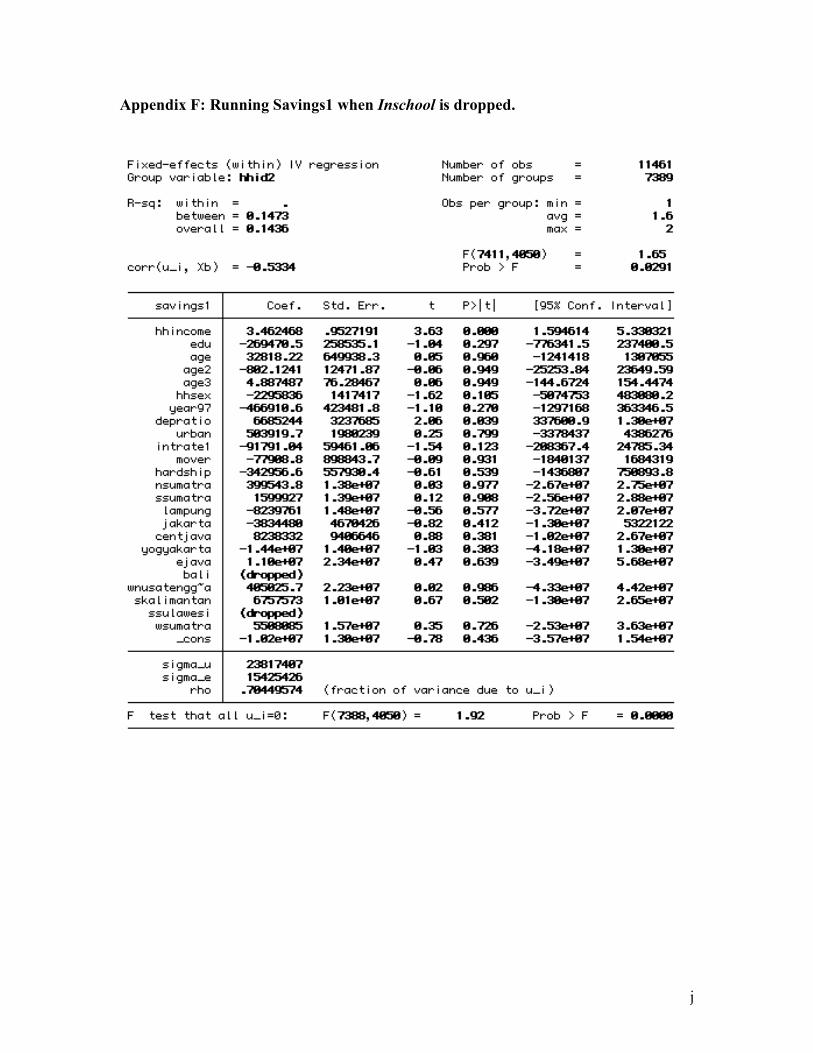
j
Appendix F: Running Savings1 when Inschool is dropped.

k
Appendix G: Results from a double log model running the log of Savings1 and the log of HHincome. The F-statistic is insignificant, hence the results are invalid.

l
Appendix H: Summary Statistics