FEDERAL RESERVE BANK OF SAN FRANCISCO

WORKING PAPER SERIES

Working Paper 2007-25 http://www.frbsf.org/publications/economics/papers/2007/wp07-25bk.pdf

The views in this paper are solely the responsibility of the authors and should not be interpreted as reflecting the views of the Federal Reserve Bank of San Francisco or the Board of Governors of the Federal Reserve System.

Examining the Bond Premium Puzzle with a DSGE Model

Glenn D. Rudebusch

Federal Reserve Bank of San Francisco

Eric T. Swanson Federal Reserve Bank of San Francisco

July 2008

Examining the Bond Premium Puzzlewith a DSGE Model∗

Glenn D. Rudebusch Eric T. Swanson†

Federal Reserve Bank of San Francisco,101 Market Street, San Francisco, CA 19105, USA

July 2008

Forthcoming in the Journal of Monetary Economics

AbstractThe basic inability of standard theoretical models to generate a sufficiently large andvariable nominal bond risk premium has been termed the “bond premium puzzle.” Weshow that the term premium on long-term bonds in the canonical dynamic stochasticgeneral equilibrium (DSGE) model used in macroeconomics is too small and stablerelative to the data. We find that introducing long-memory habits in consumption aswell as labor market frictions can help fit the term premium, but only by seriouslydistorting the DSGE model’s ability to fit other macroeconomic variables, such as thereal wage; therefore, the bond premium puzzle remains.

JEL classification: E43; G12

Keywords: yield curve; term premium; bond pricing

∗For helpful comments, we thank participants at the conference honoring John Taylor held at the FederalReserve Bank of Dallas in 2007, especially our discussant Monika Piazzesi, and participants at the 2007NBER Summer Institute session on DSGE modeling, the 2007 Dynare annual conference in Paris, and the2008 London School of Economics conference on macroeconomics, as well as many colleagues in the FederalReserve System. Anjali Upadhyay provided excellent research assistance. The views expressed in this paperare those of the authors and do not necessarily reflect the views of other individuals within the FederalReserve System.†Corresponding author. Tel.: + 1 415 974 3172. E-mail address: eric.swanson@sf.frb.org (E. Swanson).

1 Introduction

Understanding the risk premium on long-term bonds is of clear practical importance. For

example, central banks around the world use the yield curve to help assess market expec-

tations about future interest rates and inflation as well as to evaluate the overall stance of

monetary policy, but they have long recognized that such information can be obscured by

time-varying risk premiums.1 Increasingly, central banks also use dynamic stochastic general

equilibrium (DSGE) models with interest rate policy rules to think about the consequences

of alternative policy actions in a rational expectations setting. These DSGE models can

make predictions about the expectational and term premium components in bond yields;

thus, it is natural to examine the extent to which these predictions are consistent with the

observed data. Accordingly, we attempt to account for the observed size and volatility of the

risk premium on long-term nominal bonds using a fairly wide variety of alternative DSGE

model specifications that have been proposed in the literature.

Early work on bond pricing by Backus, Gregory, and Zin (1989) examined the bond

premium using a consumption-based asset pricing model of an endowment economy. They

found that “the representative agent model with additively separable preferences fails to

account for the sign or the magnitude of risk premiums” and “cannot account for the vari-

ability of risk premiums” (p. 397). This basic inability of a standard theoretical finance

model to generate a sufficiently large and variable nominal bond risk premium has been

termed the “bond premium puzzle.” Subsequently, Donaldson, Johnson, and Mehra (1990)

and Den Haan (1995) showed that the bond premium puzzle is likewise present in standard

real business cycle models with variable labor and capital and with or without simple nominal

rigidities. Since these early studies, however, the “standard” theoretical model in macroe-

conomics has undergone dramatic changes and now includes a prominent role for habits in

consumption and nominal rigidities that persist for several periods (such as staggered Taylor

(1980) or Calvo (1983) price contracts), both of which should help the model to account

1 Notably, in 2004 and 2005, as long- and short-term interest rates diverged—the so-called bond yield“conundrum”—measures of the size of the risk premium on long-term nominal bonds attracted widespreadattention (see Rudebusch, Swanson, and Wu, 2006, and Smith and Taylor, 2007).

1

for the term premium. Christiano, Eichenbaum, and Evans (2005) and Smets and Wouters

(2003) have shown that DSGE models with these features can match the impulse responses

of the economy to nominal shocks and technology shocks better than the earlier generation of

models. We investigate whether these models are likewise better able to match the price and

risk premium on a long-term nominal bond. To preview our results, we find that the bond

premium puzzle remains in state-of-the-art macroeconomic DSGE models, even when these

models are extended to include large and persistent habits as in Campbell and Cochrane

(1989) and Wachter (2006) and real wage bargaining rigidities as in Blanchard and Galı

(2005). That is, these models are still very far from matching the level and variability of

the term premium, the slope of the yield curve, and the excess returns to holding long-term

bonds that we see in the data.

The importance of jointly modeling both macroeconomic variables and asset prices within

a DSGE framework is sometimes underappreciated. Indeed, a standard research tack has

been to use DSGE models to explain the behavior of macroeconomic variables and latent-

factor finance models to fit asset prices, but this dichotomous modeling approach suffers

from at least two serious shortcomings.2 First, as a theoretical matter, asset prices and

the macroeconomy are inextricably linked, so a failure of the standard DSGE framework

to explain asset prices suggests flaws in the model. As emphasized by Cochrane (2007),

asset markets are the mechanism by which consumption and investment are allocated across

time and states of nature, so asset prices, which equate marginal rates of substitution and

transformation, are at the very foundation of the dynamics of macroeconomic quantities.

If a DSGE model can match the data on macroeconomic quantities but not asset prices,

then how does the model propose that marginal rates of substitution and transformation

are being equated? Surely, such behavior is a sign that the model itself is flawed or at

least incomplete. Second, from a practical point of view, policymakers and others are often

very interested in the interaction between macroeconomic variables and asset prices—both

the effects of asset prices on macro variables and the effects of interest rates and other

2 These shortcomings have fostered a greater emphasis in the literature on the importance of macro-financelinkages, for example, Ang and Piazzesi (2003) and Diebold, Piazzesi, and Rudebusch (2005).

2

macro variables on asset prices. For example, a question of recent interest is how does

a seemingly very low term premium—the bond yield “conundrum”—affect the economy.

As Rudebusch, Sack, and Swanson (2007) discuss, this question cannot be addressed with

a dichotomous macroeconomic and financial modeling approach; it requires a structural

macro-finance model.

Although the bond premium puzzle has received far less attention in the literature than

Mehra and Prescott’s (1985) equity premium puzzle, it is in fact just as interesting and

important. Indeed, as a practical matter, the value of long-term bonds outstanding in the

U.S. is far larger than the value of equities. In addition, from a modeling perspective, the

bond premium puzzle provides a very different metric for model performance. For example,

Boldrin, Christiano, and Fisher (2001) can account for the equity premium puzzle in a two-

sector DSGE model because capital immobility across the two sectors greatly increases the

variance of the price of capital (and thus stock prices) and its covariance with consumption.

However, this mechanism cannot explain the bond premium puzzle, which involves the val-

uation of a constant nominal coupon on a default-free government bond. In contrast to the

equity premium puzzle, the bond premium puzzle is intimately related to the behavior of

inflation, nominal rigidities, and nominal asset prices, which are crucial and still unresolved

aspects of the current generation of DSGE models.

The bond premium puzzle has also attracted renewed interest in the finance and macro

literatures. Wachter (2006) and Piazzesi and Schneider (2006) have had notable success in

resolving this puzzle within an endowment economy by using preferences that have been

modified to include either an important role for habit, as in Campbell and Cochrane (1999),

or “recursive utility,” as in Epstein and Zin (1989). While such success in an endowment

economy is encouraging, it is somewhat unsatisfying because, as noted above, the lack of

structural relationships between the macroeconomic variables precludes studying many ques-

tions of interest. Accordingly, there has been interest in extending the endowment economy

results to more fully specified DSGE models.3 Wu (2006), Bekaert, Cho, and Moreno (2005),

3 Hordahl, Tristani, and Vestin (2006), Rudebusch and Wu (2007), and other macro-finance researchershave examined term premiums with an affine no-arbitrage structure and a log-linearized version of a DSGE

3

Hordahl, Tristani, and Vestin (2007), and Doh (2006) use the stochastic discount factor from

a standard DSGE model to study the term premium, but to solve the model, these authors

have essentially assumed that the term premium is constant over time—that is, they have

essentially assumed the expectations hypothesis.4 Since we are interested in the variability

as well as the level of the term premium, and in the relationship between the term premium

and the macroeconomy, a higher-order approximate solution method or a global nonlinear

method is required, as in Ravenna and Seppala (2006), Rudebusch, Sack, and Swanson

(2007), and Gallmeyer, Hollifield, and Zin (2005).5 Still, as we discuss in detail below, these

last authors have had mixed success in solving the bond premium puzzle, and in particular,

it remains unclear whether the size and volatility of the bond premium can be replicated

in a DSGE model without distorting its macroeconomic fit and stochastic moments. Our

analysis sheds light on this issue.

Our paper also has some similarities with the equity premium studies of Jermann (1998)

and Lettau and Uhlig (2000). Just as those authors raise questions about the ability of

Campbell and Cochrane’s (1999) habit specification to match the equity premium in a real

business cycle model, our results raise serious questions about the ability of standard macroe-

conomic habit specifications, and the Campbell and Cochrane (1999) and Wachter (2006)

extensions of that specification, to match the nominal asset pricing facts. Our results build

on the earlier work by considering nominal bond prices in a modern DSGE model with a

central role for nominal rigidities, labor market frictions, and habits in consumption, such as

model. However, these models employ an exogenous stochastic pricing kernel that does not enforce a con-sistency between the asset pricing structure and the utility function underlying the macro structure.

4 Wu (2006) and Bekaert, Cho, and Moreno (2005) use a log-linear, log-normal approximation to solvethe model, which allows some second- and higher-order terms from the log-normal distribution to remain inthese models, although the implied term premium is constant. An additional drawback of their approach isthat it treats some second-order terms as important while dropping other terms of similar magnitude. Incontrast, Hordahl, Tristani, and Vestin (2006b), compute a full second-order approximate solution to themodel, which treats all second-order terms equally; however, the term premium is also a constant in thisapproach, as we discuss below. Doh (2006) does allow for a time-varying term premium, but does so bycombining a full second-order solution with an ARCH process on one of the shocks, which again treats somethird- and higher-order terms as being important while dropping other terms of similar magnitude.

5 Ravenna and Seppala (2006) and Rudebusch, Sack, and Swanson (2007) use a third-order approximatesolution to the model, which allows for a time-varying term premium. Gallmeyer, Hollifield, and Zin (2005)are able to compute a closed-form solution for bond prices for a very special monetary policy reactionfunction, but their method does not apply to more general monetary policy reaction functions such as theTaylor policy rule we consider below.

4

Christiano, Eichenbaum, and Evans (2005). We show that even such state-of-the-art macro

models fall egregiously short of being able to price nominal assets. Our results suggest that

non-habit-based modifications of the model, such as Epstein-Zin (1989) and Weil (1989)

recursive preferences, may be more promising extensions of DSGE models to asset pricing.

In the next section, we introduce our benchmark DSGE model, which is set well within

the broad range of the literature, and show how to derive the term premium and other

measures of long-term bond risk in the model. Section 3 compares the implications of the

model to the data and shows that the term premium in the model is counterfactually small

and stable. Section 4 explores whether long-memory habits, as in Campbell and Cochrane

(1999), can help the model to explain the term premium, and Section 5 considers whether

adding labor market frictions to the model might improve its fit. Section 6 concludes.

2 A Benchmark DSGE Model

We begin our investigation by outlining a standard benchmark DSGE model with nominal

rigidities. We then define the term premium on a long-term bond and several other common

measures that can be used to assess the bond market performance of a model. Finally, we

describe our solution methods.

2.1 The Benchmark Model

The economy contains a continuum of households with a total mass of unity. Households are

representative and seek to maximize utility over consumption and labor streams given by

maxEt

∞∑t=0

βt(

(ct − bht)1−γ

1− γ− χ0

l1+χt

1 + χ

), (1)

where β denotes the household’s discount factor, ct denotes consumption in period t, lt

denotes labor, ht denotes a predetermined stock of consumption habits, and γ, χ, χ0, and

b are parameters. In our baseline specification, we will set ht = Ct−1, the level of aggregate

consumption in the previous period (so the habit stock is external to the household), although

5

we will consider alternative formulations such as long-memory habits and internal habits

later. The household’s nominal stochastic discount factor from period t to t + j in this

model thus satisfies

mt,t+j ≡ βj(ct+j − bCt+j−1)

−γ

(ct − bCt−1)−γPtPt+j

. (2)

The economy also contains a continuum of monopolistically competitive intermediate

goods firms indexed by f ∈ [0, 1] that set prices according to Calvo contracts and hire labor

competitively from households. Firms have Cobb-Douglas production functions:

yt(f) = Atk(1−α)

lt(f)α, (3)

where k is a fixed, firm-specific capital stock (identical across firms) and where At denotes an

aggregate technology shock that affects all firms.6 The level of aggregate technology follows

an exogenous AR(1) process:

logAt = ρA logAt−1 + εAt , (4)

where εAt denotes an i.i.d. aggregate technology shock with mean zero and variance σ2A.

Intermediate goods are purchased by a perfectly competitive final goods sector that

produces the final good with a CES production technology:

Yt =

[∫ 1

0

yt(f)1/(1+θ)df

]1+θ

. (5)

Each intermediate goods firm f thus faces a downward-sloping Dixit-Stiglitz demand curve

for its product and the aggregate price level Pt is defined to be the Dixit-Stiglitz price

aggregate.

Each firm sets its price pt(f) according to a Calvo contract that expires with probability

1 − ξ each period, with no indexation. Firms hire labor lt(f) from households in a com-

petitive labor market, paying the nominal market wage wt. Firms are collectively owned by

households and distribute profits and losses back to the households. When a firm’s price

6 Several authors, such as Woodford (2003) and Altig, Christiano, Eichenbaum, and Linde (2004), haveemphasized the importance of firm-specific fixed factors for generating a level of inflation persistence that isconsistent with the data. With firm-specific capital stocks, the term premium is higher as well as inflationbeing more persistent.

6

contract expires and it is able to set a new contract price, the firm maximizes the expected

present discounted value of profits over the lifetime of the contract, using the representative

household’s stochastic discount factor (2) to value future profits. Firms’ optimality condi-

tions and the aggregate resource constraints in this model are standard and are described in

the appendix to Rudebusch, Sack, and Swanson (2007).

Although agents cannot invest in physical capital in the baseline version of the model,

we do assume that an amount δK of output each period is devoted to maintaining the

fixed capital stock. Households can also buy and sell one-period risk-free nominal bonds,

subject to an individual borrowing constraint that is not binding but rules out Ponzi schemes.

Optimizing behavior by households gives rise to the intratemporal condition

wtPt

=χ0l

χt

(ct − bCt−1)−γ, (6)

and the intertemporal Euler equation

(ct − bCt−1)−γ = βeitEt(ct+1 − bCt)−γPt/Pt+1, (7)

where it denotes the continuously compounded interest rate on the one-period risk-free nom-

inal bond.

The government levies lump-sum taxes Gt on households and destroys the resources it

collects. The aggregate resource constraint implies that

Yt = Ct + δK +Gt, (8)

where Ct = ct, the consumption of the representative household. Government consumption

follows an exogenous AR(1) process:

logGt = ρG logGt−1 + εGt , (9)

where εGt denotes an i.i.d. government consumption shock with mean zero and variance σ2G.

Finally, there is a monetary authority in the economy which sets the one-period nominal

interest rate it according to a Taylor-type policy rule:

it = ρiit−1 + (1− ρi)[1/β + πt + gy(Yt − Y )/Y + gπ(πt − π∗)

]+ εit, (10)

7

where 1/β is the steady-state real interest rate in the model, Y denotes the steady-state

level of output, π∗ denotes the steady-state rate of inflation, εit denotes an i.i.d. stochastic

monetary policy shock with mean zero and variance σ2i , and ρi, gy, and gπ are parameters.7

The variable πt denotes a geometric moving average of inflation:

πt = θππt−1 + (1− θπ)πt, (11)

where current-period inflation πt ≡ log(Pt/Pt−1) and we set θπ = 0.7 so that the geometric

average in (11) has an effective duration of about four quarters, which is typical in estimates

of the Taylor Rule. The advantage of using (11) rather than the four-quarter average inflation

rate is that (11) only requires keeping track of one lagged variable (πt−1) and hence one extra

state variable in the model, while a four-quarter moving average would require keeping track

of three (πt−1, πt−2, and πt−3). All of our results below are very similar whether we use (11)

or a more traditional four-quarter average inflation rate in the policy rule (10).

2.2 The Term Premium in the Model

The price of any asset in the model economy must satisfy the standard stochastic discounting

relationship in which the household’s stochastic discount factor is used to value the state-

contingent payoffs of the asset in period t + 1. For example, the price of a default-free

n-period zero-coupon bond that pays one dollar at maturity satisfies:

p(n)t = Et[mt+1p

(n−1)t+1 ], (12)

where mt+1 ≡ mt,t+1, p(n)t denotes the price of the bond at time t, and p

(0)t ≡ 1, i.e., the

time-t price of one dollar delivered at time t is one dollar. The continuously-compounded

yield to maturity on the n-period zero-coupon bond is defined to be:

i(n)t ≡ −

1

nlog p

(n)t . (13)

7 In equation (10) (and equation (10) only), we express it, πt, and 1/β in annualized terms, so thatthe coefficients gπ and gy correspond directly to the estimates in the empirical literature. We also followthe literature by assuming an “inertial” policy rule with i.i.d. policy shocks, although there are a varietyof reasons to be dissatisfied with the assumption of AR(1) processes for all stochastic disturbances exceptthe one asociated with short-term interest rates. Indeed, Rudebusch (2002, 2006) and Carrillo, Feve, andMatheron (2007) provide strong evidence that an alternative policy specification with serially correlatedshocks and little gradual adjustment is more consistent with the dynamic behavior of nominal interest rates.

8

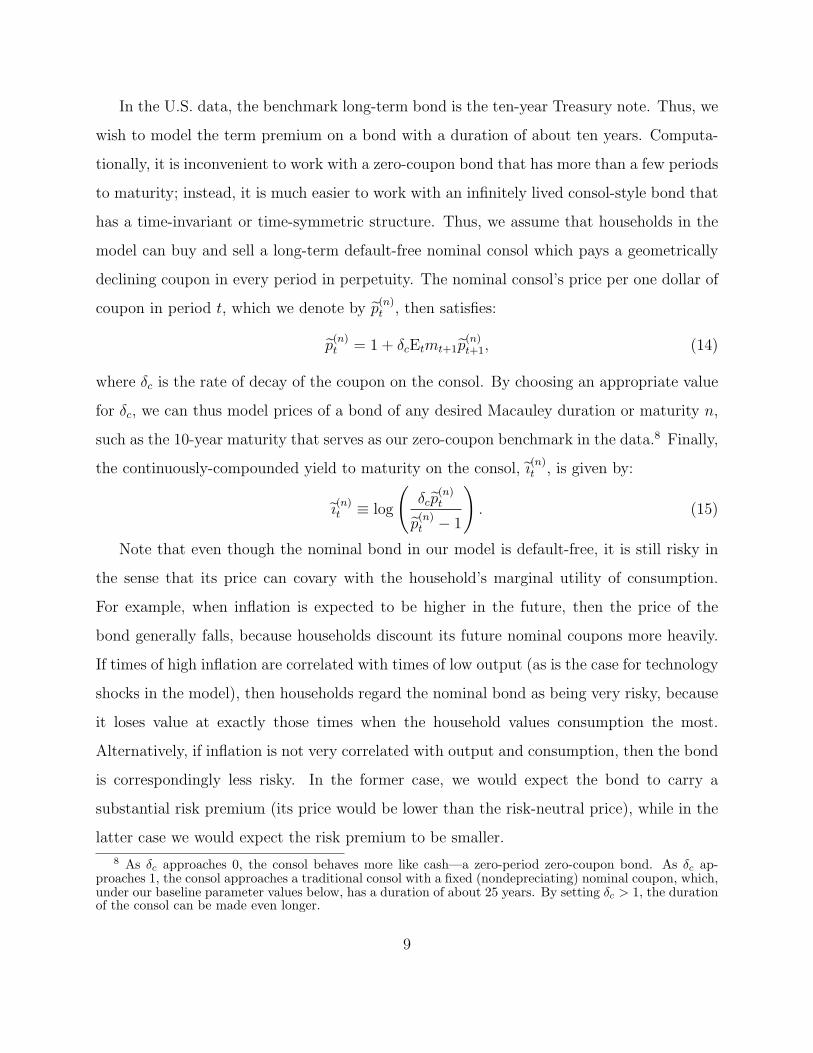
In the U.S. data, the benchmark long-term bond is the ten-year Treasury note. Thus, we

wish to model the term premium on a bond with a duration of about ten years. Computa-

tionally, it is inconvenient to work with a zero-coupon bond that has more than a few periods

to maturity; instead, it is much easier to work with an infinitely lived consol-style bond that

has a time-invariant or time-symmetric structure. Thus, we assume that households in the

model can buy and sell a long-term default-free nominal consol which pays a geometrically

declining coupon in every period in perpetuity. The nominal consol’s price per one dollar of

coupon in period t, which we denote by p(n)t , then satisfies:

p(n)t = 1 + δcEtmt+1p

(n)t+1, (14)

where δc is the rate of decay of the coupon on the consol. By choosing an appropriate value

for δc, we can thus model prices of a bond of any desired Macauley duration or maturity n,

such as the 10-year maturity that serves as our zero-coupon benchmark in the data.8 Finally,

the continuously-compounded yield to maturity on the consol, ı(n)t , is given by:

ı(n)t ≡ log

(δcp

(n)t

p(n)t − 1

). (15)

Note that even though the nominal bond in our model is default-free, it is still risky in

the sense that its price can covary with the household’s marginal utility of consumption.

For example, when inflation is expected to be higher in the future, then the price of the

bond generally falls, because households discount its future nominal coupons more heavily.

If times of high inflation are correlated with times of low output (as is the case for technology

shocks in the model), then households regard the nominal bond as being very risky, because

it loses value at exactly those times when the household values consumption the most.

Alternatively, if inflation is not very correlated with output and consumption, then the bond

is correspondingly less risky. In the former case, we would expect the bond to carry a

substantial risk premium (its price would be lower than the risk-neutral price), while in the

latter case we would expect the risk premium to be smaller.

8 As δc approaches 0, the consol behaves more like cash—a zero-period zero-coupon bond. As δc ap-proaches 1, the consol approaches a traditional consol with a fixed (nondepreciating) nominal coupon, which,under our baseline parameter values below, has a duration of about 25 years. By setting δc > 1, the durationof the consol can be made even longer.

9

In the literature, the risk premium or term premium on a long-term bond is typically

expressed as the difference between the yield on the bond and the unobserved risk-neutral

yield for that same bond. To define the term premium in our model, then, we first define

the risk-neutral price of the consol, p(n)t :

p(n)t ≡ Et

∞∑j=0

e−it,t+jδjc , (16)

where it,t+j ≡∑j

n=0 in. Equation (16) is the expected present discounted value of the coupons

of the consol, where the discounting is performed using the risk-free rate rather than the

household’s stochastic discount factor.9 Equivalently, equation (16) can be expressed in

first-order recursive form as:

p(n)t = 1 + δce

−itEtp(n)t+1, (17)

which directly parallels equation (14). The implied term premium on the consol is then given

by:

ψ(n)t ≡ log

(δcp

(n)t

p(n)t − 1

)− log

(δcp

(n)t

p(n)t − 1

), (18)

which is the difference between the observed yield to maturity on the consol and the risk-

neutral yield to maturity.

For a given set of structural parameters of the model, we will choose δc so that the bond

has a Macauley duration of n = 40 quarters, and we will multiply equation (18) by 400 in

order to report the term premium in units of annualized percentage points rather than logs.

9 In computing the term premium, some authors take the expectation over yields rather than over prices(with the difference between the two approaches being a convexity term). Equation (16) follows the no-aribtrage finance and macro-finance literatures (e.g., Ang and Piazzesi, 2003), which compute risk-neutralbond prices by setting the prices of risk to zero. An alternative definition of the risk-neutral bond price,suggested to us by Oreste Tristani, would consider what value a single hypothetical agent with utility function(1) and γ = 0 would assign to the bond. This definition is problematic, however, because the risk-neutralagent has an intertemporal elasticity of substitution that differs from that of the representative agent in theeconomy, which implies that the risk-neutral agent and representative agents have different one-period risk-free rates after a shock. Thus, even in a riskless world, this alternative definition would imply a time-varying“term premium”. Our definition appears more consistent with the finance and macro-finance literatures.

10

2.3 Alternative Measures of Long-Term Bond Risk

Although the term premium is the cleanest conceptual measure of the riskiness of long-term

bonds, it is not directly observed in the data and must be inferred using term structure models

or other methods. Accordingly, the literature has also focused on three other empirical

measures that are closely related to the term premium but are more easily observed: the

slope of the yield curve, the excess return to holding the long-term bond for one period

relative to the one-period short rate, and the slope coefficient from a Campbell-Shiller (1991)

predictability regression of the change in the long-term yield on the yield curve slope.10 In

the next section, we will compare the model’s ability to fit the data using each of these

measures, and here we define them in more detail.

The slope of the yield curve is simply the difference between the yield to maturity on

the long-term bond and the one-period risk-free rate, it. The slope of the yield curve is an

imperfect measure of the riskiness of the long-term bond because the yield curve slope can

vary in response to shocks even if all investors in the model are risk-neutral. However, on

average, the slope of the yield curve equals the term premium, and the volatility of the yield

curve slope provides us with a noisy measure of the volatility of the term premium.

A second measure of the riskiness of long-term bonds is the excess one-period holding

return—that is, the return to holding the bond for one period less the one-period risk-free

rate. For the case of an n-period zero-coupon bond, this excess return is given by:

x(n)t ≡

p(n−1)t

p(n)t−1

− eit−1 . (19)

The first term on the right-hand side of (19) is the gross return to holding the bond and the

second term is the gross one-period risk-free return. For the case of the consol in our model,

the excess holding period return is a bit more complicated, since the consol pays a coupon

in period t − 1 and then depreciates in value by the factor δc, so the excess holding period

10 See, respectively, Piazzesi and Schneider (2006), Cochrane and Piazzesi (2005), and Rudebusch and Wu(2007).

11

return is given by:

x(n)t ≡

δcp(n)t + eit−1

p(n)t−1

− eit−1 . (20)

Again, the first term on the right-hand side of (20) is the gross return to holding the consol

and includes the one-dollar coupon in period t − 1 that can be invested in the one-period

security. As with the yield curve slope, the excess returns in (19) and (20) are imperfect

measures of the term premium because they would vary in response to shocks even if investors

were risk-neutral. However, the mean and standard deviation of the excess holding period

return provide popular measures of the average term premium and the volatility of the term

premium.

A third measure of bond risk is based on the “long-rate regression” popularized by Camp-

bell and Shiller (1991):

i(n−1)t+1 − i(n)

t = α(n)CS + β

(n)CS

i(n)t − itn− 1

+ ε(n)t+1, (21)

where the dependent variable is the change in the n-period zero–coupon yield from period t

to t+ 1, the independent variable is the yield curve slope at time t (divided by n− 1), and

α(n)CS and β

(n)CS are maturity-specific intercept and slope coefficients. Under the expectations

hypothesis, expected excess returns (19) are zero, that is:

log p(n−1)t+1 − log p

(n)t = it. (22)

After substituting the definition (13) and rearranging terms, (22) would imply that the

coefficients β(n)CS = 1 and α

(n)CS = 0; that is, the yield curve slope is the optimal forecast of the

future change in the long rate. Deviations from risk neutrality drive α(n)CS away from zero,

and time-variation in the term premium pushes β(n)CS away from unity. Note that (21) could

equivalently be written and run as:

log p(n)t

n−

log p(n−1)t+1

n− 1= α

(n)CS + β

(n)CS

i(n)t − itn− 1

+ ε(n)t+1, (23)

which turns out to be the more useful format for the consol below.

12

For the consol in our model, the derivation of the Campbell-Shiller regression coefficient

is a bit more complicated, reflecting the extra terms in (20) relative to (19). Instead of (22),

the appropriate equation is

log(δcp(n)t+1 + eit)− log p

(n)t = it. (24)

After substituting the definition (15) and rearranging terms, this implies:

log p(n)t − log p

(n)t+1 = ı

(n)t − it. (25)

Thus, the Campbell-Shiller regression for the consol in the model is most simply written as:

log p(n)t − log p

(n)t+1 = α

(n)CS + β

(n)CS (ı

(n)t − it) + ε

(n)t+1, (26)

where the coefficients α(n)CS and β

(n)CS in the model have exactly the same interpretation as in

the data.

2.4 Model Solution Method

A technical issue in solving the model above arises from the relatively large number (nine)

of state variables—Ct−1, At−1, Gt−1, it−1, ∆t−1, πt−1, and the three shocks, εAt , εGt , and, εit.11

Because of such high dimensionality, value-function iteration-based methods such as pro-

jection methods (or, even worse, discretization methods) are computationally intractable.

We instead solve the model using the standard macroeconomic technique of approxima-

tion around the nonstochastic steady state—so-called perturbation methods. However, a

first-order approximation of the model (i.e., a linearization or log-linearization) eliminates

the term premium entirely, because equations (14) and (17) are identical to first order, a

manifestation of the well-known property of certainty equivalence in linearized models. A

second-order approximation to the solution of the model produces a term premium that is

nonzero but constant (a weighted sum of the variances σ2A, σ2

G, and σ2i ). Since our interest in

11 The number of state variables can be reduced a bit by noting that Gt and At are sufficient to incorporateall of the information from Gt−1, At−1, εGt , and εAt , but the basic point remains valid, namely, that thenumber of state variables in the model is large from a computational point of view.

13

this paper is not just in the level of the term premium but also in its volatility and variation

over time, we must compute a third-order approximate solution to the model around the

nonstochastic steady state. We do so using the nth-order perturbation AIM algorithm of

Swanson, Anderson, and Levin (2006), which automatically and quickly computes nth-order

approximate solutions to dynamic discrete-time rational expectations models of this type.

For the baseline model above with nine state variables, a third-order accurate solution can

be computed in about ten minutes on a standard laptop computer. Additional details of

this solution method are provided in Swanson, Anderson, and Levin (2006) and Rudebusch,

Sack and Swanson (2007).

Once we have computed an approximate solution to the model, we compare the model

and the data using a standard set of macroeconomic and financial moments, including the

standard deviations of consumption, labor, and other variables, and the means and stan-

dard deviations of the term premium and the alternative measures of long-term bond risk

described above. Because our approximate solution to the model is nonlinear, we com-

pute these moments from synthetic model data. (Namely, beginning from the nonstochastic

steady state, we simulate the model forward 500,000 observations using normally distributed

shocks.)

3 Comparing the Model to the Data

How well can the benchmark DSGE model fit the first and second empirical moments of

macroeconomic and financial variables? We begin with a baseline parameterization of the

DSGE model drawn from the literature. Since this standard parameterization is unable to

fit the empirical facts, we then explore alternatives that may help the model fit the data.

3.1 Baseline Model Parameterization and Sensitivity Analysis

The baseline set of parameter values with which we begin our analysis are reported in the

first column of Table 1 and are typical of those in the literature (see, e.g., Levin, Onatski,

14

Williams, and Williams, 2005). We set the household’s discount factor to .99 per quarter

(implying a steady-state real interest rate of 4.02 percent per year), firms’ output elasticity

with respect to labor to .7, firms’ steady-state markup to .2 (implying a price-elasticity of

demand of 6), and the average price contract duration to four quarters. The importance

of habits in the household’s utility is set to .66, consistent with typical estimates in the

macro literature. We set the utility curvature parameter γ to 2, which is a little on the high

side of standard macroeconomic estimates, to give the model a better chance of generating

an appreciable term premium. We set the utility curvature parameter on labor χ to 1.5

(implying a Frisch elasticity of about 0.7), which is again a little higher than typical macro

estimates (but in line with estimates from the labor literature) but also gives the model a

better chance of matching the term premium. The shock persistences ρA and ρG are set to

0.9, as is common, and the shock variances σ2A and σ2

G are set to .012 and .0042, respectively,

consistent with typical estimates in the literature. The monetary policy rule coefficients are

taken from Rudebusch (2002) and are also typical of those in the literature. We assume

the steady-state capital-output ratio is 2.5, which is close to what is found in the data, and

steady-state government spending is about 17 percent of output. As is standard, we set the

baseline steady-state inflation rate in the model to 0 percent per year. The parameter χ0 is

chosen to normalize the steady-state quantity of labor to unity and, as discussed above, the

parameter δc is chosen to set the Macauley duration of the consol in the model to ten years.

For the model with these baseline parameter values, we compute the third-order approx-

imate solution to the model as well as various model-implied moments by simulation. The

results of this exercise are reported in the first two columns of Table 2, along with the cor-

responding empirical moments for quarterly U.S. data from 1960 to 2007. For the empirical

moments, consumption is real personal consumption expenditures from the U.S. national

income and product accounts, labor is total hours of production workers from the Bureau of

Labor Statistics, and the real wage is total wages and salaries of production workers from the

BLS divided by total production worker hours and deflated by the GDP price index. The

standard deviation was computed for logarithmic deviations of each series from a flexible HP

15

trend and reported in percentage points. Standard deviations for inflation, interest rates, and

the term premium were computed for the raw series rather than for deviations from trend.

Inflation is the annualized rate of change in the quarterly GDP price index from the Bureau

of Economic Analysis. The short-term nominal interest rate i is the end-of-month federal

funds rate from the Federal Reserve Board, in annualized percentage points. The short-term

real interest rate r is the short-term nominal interest rate less the realized quarterly inflation

rate. The ten-year zero-coupon bond yield is the end-of-month ten-year zero-coupon bond

yield taken from Gurkaynak, Sack, and Wright (2008). The term premium on the ten-year

zero-coupon bond is the term premium computed by Kim and Wright (2005), in annualized

percentage points.12 The yield curve slope, one-period excess holding return, and Campbell-

Shiller coefficient are from the authors’ calculations based on the data above; the yield curve

slope and one-period excess holding return are reported in annualized percentage points.

As can be seen in Table 2, for the benchmark model with standard parameter values, the

average term premium is a bit less than 1.4 basis points, and the standard deviation of the

term premium is around 0.1 basis point, both roughly two orders of magnitude smaller than

the data.13 The results are basically no better for the yield curve slope or excess holding

period return measures—although the standard deviations of these variables are greater than

zero, that variation is due entirely to the risk-neutral components of those variables rather

than any variation in the riskiness of the long-term bond. By any measure, the long-term

bond in the model is priced essentially risk-neutrally, resulting in term premia and other

measures of bond risk that are negligible.

Although the benchmark DSGE model that we have used to conduct this experiment is

fairly simple, we have obtained similar results from more complicated DSGE models in the

literature. For example, in the moderately-sized DSGE model of Christiano, Eichenbaum,

12 Kim and Wright (2005) use an arbitrage-free, three-latent-factor affine model of the term structure tocompute the term premium. Alternative measures of the term premium using a wide variety of methodsproduce qualitatively similar results in terms of the overall magnitude and variability—see Rudebusch, Sack,and Swanson (2007) for a detailed discussion and comparison of several methods.

13 The lack of variation in the baseline model’s estimate of the term premium is also illustrated by itsimpulse response to economic shocks. For example, the term premium moves less than five one-hundredths ofone basis point on impact in response to a 1 percent technology shock and decays thereafter. See Rudebusch,Sack, and Swanson (2007) for further discussion.

16

and Evans (2005), the mean term premium is just 1 basis point—even smaller than in our

benchmark model.14 In the Levin, Onatski, Williams, and Williams (2006) version of the

Smets-Wouters (2003) model, which has a greater number of shocks with high persistence

and variance, the mean term premium is just 2.1 basis points.

From the point of view of a second- or third-order approximation to a macroeconomic

model, these results should not be too surprising. The shocks in the benchmark model

have a standard deviation of only about 1 percent, so first-order terms in the model have

a magnitude that is roughly proportional to (.01), second-order terms have a magnitude

that is roughly proportional to (.01)2, where the constant of proportionality is related to the

curvature of the model, and third-order terms have a magnitude that is roughly proportional

to (.01)3. Because the shocks in a macro model like our benchmark model are typically so

small, the second-order terms should be expected to be roughly 100 times smaller than the

first-order terms for a relatively flat model, and the third-order terms should be expected to

be roughly 10,000 times smaller. Only for an extremely curved model, or for much larger

shock standard deviations, could we reasonably expect the second- or third-order terms to

matter very much.

This basic intuition is supported by the sensitivity analysis we conduct in the remaining

columns of Table 1. In each row of the table, we vary each parameter in turn over a wide

range that broadly covers the empirical estimates of the parameter in the literature, to

see if any of these variations causes the mean term premium to change substantially. (To

conserve space, we do not report the alternative measures of bond risk, but they are always

similar in magnitude to the mean term premium.) The middle columns of Table 1 report

the mean term premium that results from using the “low” value for each parameter, and the

rightmost columns report the mean term premium that results from using the “high” value

(as each parameter is varied, the other parameters are held fixed at their baseline values).

For example, setting α = .5 instead of .7 reduces the mean term premium to 1.3 basis points,

14 In contrast to Christiano, Eichenbaum, and Evans (2005), we assume that the central bank follows aTaylor-type reaction function for the short-term nominal interest rate (equation (18)) rather than a moneygrowth rule. This modification to the model is standard practice in the large-scale DSGE models being putinto practice at central banks and the IMF, among others.

17

while setting α = .85 increases it to 1.5 basis points. Across all of these parameter variations,

the mean term premium is always at least an order of magnitude too small relative to the

data. Still, in line with the intuition above, some parameters are more important than

others. In particular, the mean term premium appears most sensitive to the variance and

persistence of the technology shock (σ2A and ρA) and to the curvature of the utility function

(γ and χ). These results foreshadow the two main approaches to increasing risk premiums

in DSGE models, which we will discuss below.

3.2 Increased Shock Volatility

As suggested by the preceding discussion and Table 1, a simple way to increase the term

premium in our model is to increase the size and persistence of the shocks. Indeed, two

recent papers, by Hordahl, Tristani, and Vestin (2007) and Ravenna and Seppala (2006), do

exactly that. In order to generate a term premium that is in line with the data, however,

both papers require extremely large shocks. For example, Hordahl et al. (HTV) assume that

the technology shock has a quarterly standard deviation of 2.37 percent and a persistence

of .986, compared with our baseline values of σA = 1 percent and ρA = .9. Adopting the

two HTV parameter values in our model (while holding all other parameters fixed at their

baseline values) increases the mean term premium from 1.4 to 69 basis points, and increases

the standard deviation of the term premium from 0.1 to 151 basis points, both of which

are much closer to the empirical estimates in Table 2. However, as shown in the third

column of Table 2, the increased shock volatility also increases the volatility of output and

the other macroeconomic variables in the model. For example, the unconditional standard

deviation of labor and real wages are around 10 percent, far in excess of the data, and the

unconditional standard deviation of inflation and the one-period nominal interest rate is over

15 percent.15 That is, the HTV parameterization can solve the bond premium puzzle, but

15 Hordahl, Tristani, and Vestin use a monetary policy rule that differs from our equation (10) in thattheir specification assumes ρi = 1 and has no coefficient on output growth or the output gap, in contrast tostandard estimates in the literature. Using their monetary policy rule instead of ours reduces inflation andinterest rate volatility down to more reasonable levels, but increases the volatility of consumption, output,labor, and the real wage to levels that are even higher than we report in Table 2. Note that HTV reportthe standard deviation of consumption growth implied by their model but do not report the business-cycle

18

only by sacrificing the model’s fit to the macroeconomic variables.

The results of Ravenna and Seppala (RS) are very similar, as can be seen in the fourth

column of Table 2. Instead of an unusually large technology shock, RS introduce a very

large taste shock dt into their model, where dt is an AR(1) marginal rate of substitution

shock assumed to have an out-sized quarterly standard deviation of 8 percent and a serial

correlation of .95. Introducing a taste shock dt of this size into our model leads to an average

term premium of 19 basis points and a standard deviation of the term premium of 8 bp,

closer to the empirical estimates. However, as in HTV, even this partial solution to the bond

premium puzzle produces counterfactually large volatilities for all of the macroeconomic

variables in the model.

3.3 Best-Fit Parameterization of the Model

If the standard macroeconomic parameterization produces a term premium that is too small,

and larger shock volatilities produce a reasonable term premium but destroy the fit of macroe-

conomic variables, is there some other parameterization of the model which might generate

a reasonable fit along both dimensions? To address this question, we search over the wide

range of parameter values reported in Table 1 to find the set of values that provides the best

joint fit to both the macroeconomic and term premium moments.

The computational time required to solve the model for each set of parameter values is a

few minutes, so it is generally not feasible to estimate the model using maximum likelihood

or Bayesian estimation procedures. Instead, we perform a grid search over the six parameters

in Table 1 that are among the most uncertain and appeared to be the most important for

the term premium—namely, γ, b, χ, ξ, ρA, and σA—and report the set of parameter values

that best fits the macroeconomic and financial moments in Table 2.16 We define the “best

variability of the output gap or labor or other variables such as the real wage. Our Table 2 makes it clearthat these variables are indeed extremely volatile, far more so than in the data.

16 We conducted the grid search in two stages, first searching over a coarse grid: γ ∈ {.5, 1, 1.5, 2, 2.5, 3,4, 5, 6}, b ∈ {0, .2, .4, .5, .6, .66, .7, .8, .9}, χ ∈ {.1, .5, 1, 1.5, 2, 3, 4, 5}, ξ ∈ {.5, .6, .75, .9}, ρA ∈ {.7, .8, .9, .95},and σA ∈ {.005, .0075, .01, , .015, .02}. After finding a best fit at γ = 6, b = .9, χ = 3, ξ = .6, ρA = .95,and σA = .005, we then refined the grid near this parameter vector and searched over the finer grid:γ ∈ {5, 5.25, 5.75, 6}, b ∈ {.75, .8, .85, .9, }, χ ∈ {2, 2.25, 2.5, 2.75, 3, 3.25, 3.5, 3.75, 4}, ξ ∈ {.5, .55, .6, .65, .7},ρA ∈ {.9, .95}, and σA ∈ {.005, .0075, .01, , .015, .02}.

19

fit” to be the set of parameters that matches the equally-weighted standard deviations of

consumption, labor, the real wage, inflation, the short-term nominal interest rate, short-term

real interest rate, long-term bond yield, and the mean term premium as closely as possible.17

The last column of Table 2 presents the moments from the resulting best-fitting parameter

values (which are γ = 6, b = .9, χ = 3, ξ = .65, ρA = .95, and σA = .005). With these

parameter values, the mean term premium is about 11 basis points and the unconditional

standard deviation of the term premium is about 1.3 basis points, a much better fit than

the baseline model though still too small relative to the data. To achieve this better fit, the

estimation procedure picks the highest possible curvature of the utility function with respect

to consumption, γ = 6, and b = .9, and the highest possible technology shock persistence,

ρA = .95. With these extreme parameter values, holding the technology shock standard

deviation fixed at its baseline value would result in macroeconomic moments that are too

volatile relative to the data, so the estimation chooses the lowest possible standard deviation,

σA = .005. The values χ = 3 and ξ = .65 are intermediate, reflecting the compromise between

better financial fit and worse macroeconomic fit.

Nevertheless, even for the best-fitting set of parameter values, our benchmark DSGE

model is unable to match simultaneously both the term premium and the most basic macroe-

conomic moments in the data, let alone additional macroeconomic and financial moments.

Although the best-fitting parameterization of the model improves the model’s fit to many

of the macroeconomic moments, the two moments that the model most fails to match are

the mean term premium and the variability of the long-term bond yield. To model and

eventually understand the behavior of these two variables clearly requires a more dramatic

modification to the standard DSGE model.

17 Minimizing the equal-weighted distance to these six moments provides us with a consistent estimatorof our parameters, though it is not efficient. We do not try to match both output and consumption becauseour benchmark DSGE model has a fixed capital stock and thus has nothing to say about investment, whichis the primary difference between consumption and output. We do not try to match the standard deviationof the term premium because doing so requires a third-order approximation rather than a second-orderapproximation for every iteration of the model, which increases the computation required for each iteration.We do not try to match the other bond risk measures because they are very hightly correlated with the termpremium in the model, so they do not provide additional information for the model to match.

20

4 Habit Formation and the Term Premium

Several modifications to standard models have been suggested as explanations to the equity

premium puzzle, including long-memory habit formation in consumption (Campbell and

Cochrane 1999), time-inseparable “recursive utility” preferences (Epstein and Zin 1989), and

heterogeneous agents (Constantinides and Duffie 1996, Alvarez and Jermann 2001). Since

these modifications have been relatively successful at producing substantial risk premiums

in endowment model economies, it is natural to ask whether they might help a DSGE

model match the level and volatility of the term premium. We focus on the long-memory

habit specification of Campbell and Cochrane (1999) because the standard DSGE models in

macroeconomics already include a prominent role for habit in consumption. Moving from

the standard habit specification to the Campbell-Cochrane long-memory specification habit

is a small variation that might allow the standard macroeconomic framework to fit the term

premium without significantly degrading its fit to the macroeconomic data.

Campbell and Cochrane (1999) propose replacing the standard habit preferences (1) with

a habit stock ht that has a much longer memory over past consumption, and a parameter

b that is much closer to unity, which increases the importance of habits in agents’ utility.

Moreover, to prevent current consumption from ever falling below habits (which would cross

a singularity of the utility function (1)), Campbell and Cochrane define habits implicitly

through surplus consumption st, as follows. First, define the household’s surplus consump-

tion ratio:

st ≡ct − bhtct

. (27)

The habit stock ht is assumed to be external to the household (“keeping up with Joneses”

habits), so letting capital letters denote aggregate quantities as above, household habits ht

are defined to equal the aggregate habit stock,

ht ≡Ct(1− St)

b, (28)

21

which is in turn defined implicitly by a process on St,

logSt = (1−φ) logS+φ logSt−1+

√

1− 2 log(St/S)

S− 1

[log(Ct/Ct−1)− Et−1 log(Ct/Ct−1)] ,

(29)

where φ and S are parameters. The primary advantage of this complicated definition of

habits is that it ensures household surplus consumption is always positive, which is important

when the habit stock is a large fraction of current consumption. Campbell and Cochrane

(1999) discuss the parameterization of (29) in detail, but surplus consumption and the habit

stock must be persistent (φ close to 1) to match the persistence of risk premiums and S must

be very low (the habit stock must be very large relative to consumption) to match the level

of the risk premium and keep the risk-free rate stable.

We investigate whether these long-memory habits can potentially explain the term pre-

mium by replacing the definition of ht in our benchmark model with the definition of habits

given by equations (27)–(29). In all other respects, we keep the benchmark model the

same.18 From the point of view of a Taylor series approximation, it is clear how these

Campbell-Cochrane preferences could help make second- or even third-order terms more

important. By increasing the size of habits relative to consumption (making S small), this

specification greatly increases the curvature of the household’s utility function with respect

to consumption—from a value of γ in the model with no habits or γ/(1− b) in our baseline

DSGE model, to γ/S in the model with long-memory habits. When S is small, such as the

value of .0588 calibrated by Campbell and Cochrane (1999), then the curvature of the utility

function is magnified by a factor of more than 16 as compared to a model with no habits

and by a factor of more than five relative to our baseline model. Such a large increase in the

curvature of the model should be expected to increase the importance of higher-order terms

in the Taylor series expansion.

Perhaps surprisingly, even with Campbell-Cochrane habits, our benchmark DSGE model

18 As in the baseline model, we set χ0 to normalize the quantity of labor L = 1 in steady state. However,because the marginal utility of consumption is so much higher with Campbell-Cochrane habits, the marginaldisutility of labor must also be higher to arrive at the same steady-state quantity of labor, which producesχ0 = 158.5, much larger than in the baseline version of the model.

22

is still unable to match the level and volatility of the term premium. The mean term premium

implied by this model rises to 2.7 basis points, which is still far less than the 106-basis-point

mean term premium estimated in the data. Moreover, this model does essentially no better

at matching the term premium’s volatility, as the unconditional standard deviation of the

term premium remains less than 1 basis point. As was the case for our benchmark model

in Table 1, this result is very robust—for example, it does not change if we vary each of

the model’s parameters over a wide range broadly covering the estimates in the literature,

including variations in the habit importance S as considered by Wachter (2006).19

This result stands in sharp contrast to Wachter (2006), who finds that Campbell-Cochrane

habits can match the mean term premium in an endowment economy, where the exogenous

process for consumption and inflation is estimated from the data. What can explain this

dramatic difference in conclusions? The key, as also emphasized by Boldrin, Christiano, and

Fisher (2001), Lettau and Uhlig (2000), and Jermann (1998), is that in a production-based

model, households can endogenously choose their labor-consumption tradeoff; in contrast,

in an endowment-based economy, households must consume whatever the endowment turns

out to be.20 If households are hit by a negative shock in a production-based model, they

can compensate for the shock by increasing their labor supply and working more hours. As

a result, they have the ability to insure themselves to some extent from the effects of the

shock on consumption by endogenously varying their labor supply in response. Households

in an endowment economy do not have this opportunity, so the consumption cost of shocks

in an endowment economy is correspondingly greater and risky assets thus carry a larger

risk premium. In the Campbell-Cochrane version of our benchmark model, this ability of

households to self-insure is enough to almost completely offset the large effects that those

habit preferences would otherwise have on the term premium.

19 The results of the sensitivity analysis for each parameter are not reported in the interest of space,but are availabe in the working version of this paper (Rudebusch and Swanson, 2007). Wachter (2006), incontrast to Campbell and Cochrance (1999), allows the parameter S to vary independently from the otherparameters of the model, and we consider varying S in this way as well. As with the other parameters inour model, variations in S of the magnitude considered by Wachter have only a tiny, negligible effect on theterm premium in our DSGE model.

20 In Jermann (1998), households are unable to vary their labor supply but can vary investment instead,so the basic point is the same.

23

This observation suggests that if labor in the model is not perfectly flexible or not com-

pletely within the household’s control, then the ability of households to self-insure against

shocks will be substantially diminished, and risk premiums increase toward the higher levels

in the endowment economy case. Boldrin, Christiano, and Fisher (2001) and Uhlig (2007)

have also emphasized the importance of labor market frictions for matching the equity pre-

mium in a production economy. We explore this case in the next section.

5 Labor Market Frictions and the Term Premium

Habits that are both very large and very persistent, like those in Campbell and Cochrane

(1999), are unable to solve the bond premium puzzle in a DSGE model in which labor

supply and production are endogenous. However, limiting the ability of households to vary

their labor supply through labor market frictions should improve the model’s ability to fit the

term premium. There are many ways to introduce labor market rigidities into our benchmark

DSGE model, and we consider three such frictions below. We begin with the simplest form

of labor market friction, a quadratic adjustment cost, then we consider two frictions with

more institutional realism: real wage rigidities and staggered nominal wage contracting.

5.1 Quadratic Labor Adjustment Costs

In this subsection, we consider the effects on the term premium of a quadratic adjustment

cost on changes in the quantity of labor from one period to the next. Specifically, in each

period, households must pay an adjustment cost, κ (log(lt/lt−1))2, which is proportional to

the squared log percentage change in labor from the previous quarter. Although this labor

market friction is simplistic, it is particularly useful for gaining intuition because its size

is so clearly parameterized by κ; as κ increases, it becomes more expensive for households

to insure themselves against a shock by varying their labor supply, so the magnitude of the

term premium should increase. Convex adjustment costs to labor can also be thought of as a

way of incorporating labor or leisure habits into the household’s utility function, as in Uhlig

24

(2007): under both specifications, changing labor is costly; with convex adjustment costs,

these costs are taken out of income, while with labor habits these costs are taken directly

out of utility, but there is a close correspondence between the two via the marginal utility

of income.21

Figure 1 displays the relationship between the mean term premium and κ for two versions

of our model with quadratic adjustment costs: one with Campbell-Cochrane habits and one

without. The horizontal axis measures κ in units of output cost for a 1 percent change

in labor—that is, if κ = 50Y , then a 1 percent change in labor from the previous quarter

costs households 0.5 percent of quarterly steady-state output today. The unconditional

standard deviation of labor in these models is about 2.5 percent, so a change in labor from

one quarter to the next of about 1 percent is about the right order of magnitude for this

representative-agent model. Figure 1 shows that both a moderate level of adjustment costs

and long-memory habits are necessary to generate a mean term premium that is roughly

consistent with the data. Without such habits, even extreme levels of adjustment costs to

labor do not have much of an effect on the term premium because variation in consumption

is simply not that abhorrent to households. With Campbell-Cochrane habits, consumption

variation is much more undesirable, so adjustment costs to labor quickly begin to generate a

substantial aversion by households to risky assets. Indeed, with Campbell-Cochrane habits

and adjustment costs of around 0.5 percent of output for a 1 percent change in labor (κ =

50Y ), the mean term premium in this model is 65 basis points, which is within range of the

empirical estimate in the data.

Unfortunately, adding labor adjustment costs to the model comes at a cost in terms of

fitting macroeconomic quantities. In the second column of Table 3, we report the uncon-

21 Jaccard (2007) considers an alternative habit formulation in which household utility is given by(Ctv(Lt)−ht)1−γ/(1−γ) and habits, ht, are an average of the lagged consumption-leisure composite Ctv(Lt),so although consumption and labor can vary separately, households prefer a smooth composite. We embed-ded this habit specification in our DSGE model and found that the term premium remains quite small—onthe order of a few basis points for the parameterizations in Table 1. In contrast, Jaccard appears able toproduce a sizable equity premium without extreme macroeconomic fluctuations by imposing a high utilitycurvature (γ = 10) and steady-state importance of habits (h is equal to 99.7 percent of Cv(L)). The asso-ciated effective coefficient of relative risk aversion is about 3,000 for gambles over the consumption-leisureaggregate.

25

ditional standard deviations for other macroeconomic and financial variables for the model

with Campbell-Cochrane habits and quadratic labor adjustment costs of κ = 50Y . Although

the volatility of the term premium is larger than under the baseline specification (in Table

2), so are the unconditional standard deviations of real wages, inflation, and short-term nom-

inal interest rates. The volatility of the real wage in particular is over 220 log percentage

points.22 Intuitively, the presence of labor adjustment costs along with Campbell-Cochrane

habits means that agents do not want to vary either labor or consumption in response to

a shock. Yet when there is a shock, one or the other of these two quantities must give; as

a result, the real wage must vary tremendously in order to achieve equilibrium. These large

movements in the real wage in turn cause firms’ marginal costs to be extremely volatile,

which passes through to prices and inflation. The Taylor-type policy rule implies that the

movements in inflation pass through to the short-term interest rate and the long-term bond

yield. Both the marginal utility of consumption and the long-term bond price are much

more volatile in this version of the model with adjustment costs, hence the term premium is

much greater in magnitude.

5.2 Real Wage Rigidities

Instead of simple quadratic labor adjustment costs, other approaches to modeling labor

market frictions might provide a better combination of macroeconomic and term premium

fit. Real (and nominal) wage rigidities and have been widely used in the macroeconomics

literature and, following Blanchard and Galı (2005), we introduce a wage bargaining friction

into our benchmark model. Specifically, we assume the real wage follows the process

logwrt = µ logwrt−1 + (1− µ)(logwr∗t + ω), (30)

where wr denotes the real wage, wr∗ denotes the frictionless real wage that would obtain

in the absence of the wage rigidity, ω denotes a steady-state wedge between the real wage

22 We have endeavored, without success, to find a parameterization that can deliver a large term premiumand plausible real wage volatility. For example, even after allowing for parameter variation of the type shownin Table 1 and lower adjustment costs, the volatility of the real wage is two orders of magnitude too large.

26

and households’ marginal rate of substitution, and µ denotes the sluggishness of wages in

adjusting toward the frictionless real wage. Although equation (30) does not explicitly

model Nash bargaining between workers and firms, Blanchard and Galı motivate it as a

simple friction that captures the essential features of real wage bargaining.

When we introduce equation (30) into our benchmark model, however, it turns out to

have essentially no effect on the term premium, either in our baseline parameterization of

the model or in our version with Campbell-Cochrane habits. Even in the version with C-C

habits and µ = .99—an extremely rigid real wage—the mean term premium in the model

increases from 2.7 to just 3.0 basis points. Setting µ = .999 increases the term premium to

only 3.4 basis points. Varying the parameters ω and µ over wide ranges has similarly small

effects.

Intuitively, the real wage rigidity drives up the variability of wr∗ and the household’s

marginal rate of substitution and stochastic discount factor. Ceteris paribus, increasing

the variance of the stochastic discount factor should increase the magnitude of the term

premium. However, the wage rigidity also makes firms’ marginal costs much smoother than

in the flexible-wage case; as a result, prices and inflation are much less volatile when there

are wage rigidities than when there are not. The net effect of these two opposing forces is

ambiguous, but for the wide range of parameterizations of the model we have considered,

the net effect never amounted to more than a few basis points, far short of the magnitude

we observe in the data.

Thus, real wage rigidities alone do not appear able to resolve the bond premium puzzle in

our benchmark DSGE model, even when combined with Campbell-Cochrane habits. How-

ever, if quadratic adjustment costs to labor are also added to the mix, then perhaps the real

wage rigidity would help to damp the excessive volatility of real wages of 221 percent that

we saw previously. In the fourth column of Table 3, we report the mean term premium and

unconditional standard deviations for the model with Campbell-Cochrane habits, quadratic

adjustment costs to labor of κ = 50Y , and with a real wage rigidity parameter of µ = .999 (in

the Campbell-Cochrane version of the model, the marginal rate of substitution is so volatile

27

that only with extreme degrees of wage rigidity can the variation in real wages and inflation

be brought back down to reasonable levels). While this extreme degree of wage rigidity does

bring the standard deviations of the real wage and other macroeconomic variables back to-

ward more reasonable levels, it also reduces the term premium, both in mean and standard

deviation, to a point that is still about five times smaller than in the data. Thus, not only

does the required degree of real wage rigidity appear to be implausibly large, but even as-

suming such wage rigidity, we are unable to fit both the term premium and macroeconomic

variables.

5.3 Staggered Nominal Wage Contracting

As an alternative to real wage frictions, we also consider staggered nominal wage contracts as

in Erceg, Henderson, and Levin (2000). Such contracts are prevalent in many medium- and

large-scale DSGE models, such as Christiano, Eichenbaum, and Evans (2005) and Smets and

Wouters (2003). Briefly, as in the Calvo price-contracting specification in the benchmark

model, each household is now assumed to be a monopolistic supplier of a differentiated type of

labor, which is bundled by a perfectly competitive labor market aggregator into the final labor

input that is used by firms. A critical element that maintains tractability in the model is the

assumption of complete financial markets, which allows households to trade state-contingent

securities and ensures that—despite the heterogeneity across households in the wage charged

and in hours worked—all households have identical wealth and consumption in every period

in equilibrium. This assumption is standard in the literature because keeping track of a

continuum of household-specific wealth holdings would be computationally intractable.

When we incorporate Calvo staggered nominal wage contracts into our benchmark model,

either under our baseline parameterization or with Campbell-Cochrane habits, there is again

no significant effect on the term premium. For example, in the Campbell-Cochrane version

of the model, the term premium actually decreases from 2.7 to 1.1 basis points when we add

Calvo wage contracts, and this result is robust when we vary the parameters of the model

over wide ranges. Intuitively, the assumption of complete financial markets that is required

28

for tractability in these models also has the side effect of allowing households to insure their

consumption streams through financial markets. Thus, even though most households in the

model cannot self-insure against negative shocks by working more hours, they can purchase

state-contingent claims that pay off in the event of a negative income shock and in the event

that the household is unable to reset its wage, which amounts to essentially the same thing.

Because of this assumption, households are still able to insure their consumption streams

from the consequences of negative shocks, and the term premium in the model remains very

small.

6 Conclusions

All in all, our results cast a pessimistic light on the ability of habit-based DSGE models to fit

the term premium. Even in versions of the model with large and persistent habits following

Campbell and Cochrane (2005), the ability of households to vary their labor supply and

thereby insure themselves against consumption fluctuations leads to term premiums that are

far too small and far, far too stable relative to the data. Trying to reduce households’ ability

to self-insure by introducing standard labor market frictions into the model dramatically

increases the volatility of households’ marginal rate of substitution and the real wage—and

hence marginal costs, inflation, and the short-term nominal interest rate—to a point that

is far in excess of the data. Thus, the success that Wachter (2006) reports in fitting the

term premium in an endowment economy does not appear to generalize to the standard

macroeconomic DSGE framework, where labor supply and production are endogenous.

While our results are somewhat discouraging from the point of view of habit-based DSGE

models, there are other approaches still available that might allow one to fit the term pre-

mium in a DSGE framework. First, Piazzesi and Schneider (2006) have reported success

in fitting the term premium in an endowment economy model using “generalized recursive”

preferences, as in Epstein and Zin (1989). This approach may be more promising than habits

in a DSGE setting because Epstein-Zin preferences separate the intertemporal elasticity of

29

substitution from the coefficient of relative risk aversion, which should give the model a

better chance of fitting both the macroeconomic quantities and asset prices. The methods

employed in the present paper—such as second- and third-order approximations and a gen-

eralized consol to model the term premium—can likewise be applied to the case of recursive

utility in a DSGE framework and make the solution of the term premium in such models

computationally tractable, and we have begun to explore this variation in Rudebusch and

Swanson (2008). Finally, models based on heterogeneous agents with incomplete insurance

markets, as in Constantinides and Duffie (1996) and Krebs (2007), might also be able to

explain the term premium, although merging heterogeneous-agent frameworks into standard

macroeconomic DSGE models poses a significant computational challenge at present.

30

References

[1] Altig, David, Lawrence Christiano, Martin Eichenbaum, and Jesper Linde, 2004. Firm-Specific Capital, Nominal Rigidities, and the Business Cycle. manuscript, NorthwesternUniversity.

[2] Alvarez, Fernando, and Urban Jermann, 2001. Quantitative Asset Pricing Implicationsof Endogenous Solvency Constraints. Review of Financial Studies 14, 1117–51.

[3] Ang, Andrew, and Monika Piazzesi, 2003. No-Arbitrage Vector Autoregression of TermStructure Dynamics with Macroeconomic and Latent Variables. Journal of MonetaryEconomics 50, 745–87.

[4] Backus, David, Allan Gregory, and Stanley Zin, 1989. Risk Premiums in the TermStructure. Journal of Monetary Economics 24, 371–99.

[5] Bekaert, Geert, Seonghoon Cho, and Antonio Moreno, 2005. New-Keynesian Macroe-conomics and the Term Structure. manuscript, Columbia Business School.

[6] Blanchard, Olivier, and Jordi Galı, 2005. Real Wage Rigidities and the New KeynesianModel. NBER Working Paper 11806.

[7] Boldrin, Michele, Lawrence Christiano, and Jonas Fisher, 2001. Habit Persistence, AssetReturns, and the Business Cycle. American Economic Review 91, 149–66.

[8] Calvo, Guillermo, 1983. Staggered Prices in a Utility-Maximizing Framework. Journalof Monetary Economics 12, 383–98.

[9] Campbell, John, and John Cochrane, 1999. By Force of Habit: A Consumption-BasedExplanation of Aggregate Stock Market Behavior. Journal of Political Economy 107,205–51.

[10] Carrillo, Julio, Patrick Feve, and Julien Matheron, 2001. Monetary Policy Inertia orPersistent Shocks: A DSGE Analysis. International Journal of Central Banking 3, 1-38.

[11] Christiano, Lawrence, Martin Eichenbaum, and Charles Evans, 2005. Nominal Rigiditiesand the Dynamic Effects of a Shock to Monetary Policy. Journal of Political Economy113, 1–45.

[12] Cochrane, John, 2007. Financial Markets and the Real Economy. In: Mehra, Rajnish(Ed.), Handbook of the Equity Risk Premium. Elsevier, Amsterdam, 237–330.

[13] Constantinides, George, and Darrell Duffie, 1996. Asset Pricing with HeterogeneousConsumers. Journal of Political Economy 104, 219–40.

31

[14] Den Haan, Wouter, 1995. The Term Structure of Interest Rates in Real and MonetaryEconomies. Journal of Economic Dynamics and Control 19, 909–40.

[15] Diebold, Francis, Monika Piazzesi, and Glenn D. Rudebusch, 2005. Modeling BondYields in Finance and Macroeconomics. American Economic Review, Papers and Pro-ceedings 95, 415–20.

[16] Doh, Taeyoung, 2006. What Moves the Yield Curve? Lessons from an Estimated Non-linear Macro Model. manuscript, University of Pennsylvania.

[17] Donaldson, John, Thore Johnsen, and Rajnish Mehra, 1990. On the Term Structure ofInterest Rates. Journal of Economic Dynamics and Control 14, 571–96.

[18] Epstein, Lawrence, and Stanley Zin, 1989. Substitution, Risk Aversion and the Tem-poral Behavior of Consumption and Asset Returns: A Theoretical Framework. Econo-metrica 57, 937–69.

[19] Erceg, Christopher, Dale Henderson, and Andrew Levin, 2000. Optimal Monetary Policywith Staggered Wage and Price Contracts. Journal of Monetary Economics 46, 281–313.

[20] Gallmeyer, Michael F., Burton Hollifield, and Stanley E. Zin, 2005. Taylor Rules, Mc-Callum Rules and the Term Structure of Interest Rates. Journal of Monetary Economics52, 921–50.

[21] Hansen, Gary, 1985. Indivisible Labor and the Business Cycle. Journal of MonetaryEconomics 16, 309–27.

[22] Hordahl, Peter, Oreste Tristani, and David Vestin, 2006. A Joint Econometric Model ofMacroeconomic and Term Structure Dynamics. Journal of Econometrics 131, 405–44.

[23] Hordahl, Peter, Oreste Tristani, and David Vestin, 2007. The Yield Curve and Macroe-conomic Dynamics. European Central Bank Working Paper 832.

[24] Jaccard, Ivan, 2007. Asset Pricing, Habit Memory, and the Labor Market. unpublishedmanuscript, The Wharton School.

[25] Jermann, Urban, 1998. Asset Pricing in Production Economies. Journal of MonetaryEconomics 41, 257–75.

[26] Kim, Don H., and Jonathan H. Wright, 2005. An Arbitrage-Free Three-Factor TermStructure Model and the Recent Behavior of Long-Term Yields and Distant-HorizonForward Rates. Federal Reserve Board, Finance and Economics Discussion Series 2005–33.

[27] Krebs, Tom, 2007. Job Displacement Risk and the Cost of Business Cycles. AmericanEconomic Review 97, 664–86.

32

[28] Lettau, Martin and Harald Uhlig, 2000. Can Habit Formation Be Reconciled with Busi-ness Cycle Facts? Review of Economic Dynamics 3, 79–99.

[29] Levin, Andrew, Alexei Onatski, John C. Williams, and Noah Williams, 2005. MonetaryPolicy Under Uncertainty in Micro-Founded Macroeconometric Models. NBER MacroAnnual, 229–87.

[30] Mehra, Rajnish, and Edward Prescott, 1985. The Equity Premium: A Puzzle. Journalof Monetary Economics 15, 145–61.

[31] Piazzesi, Monika, and Martin Schneider, 2006. Equilibrium Yield Curves. NBER MacroAnnual, 389–442.

[32] Ravenna, Federico, and Juha Seppala, 2006. Monetary Policy and the Term Structureof Interest Rates. manuscript, University of California, Santa Cruz.

[33] Rudebusch, Glenn D., 2002. Term Structure Evidence on Interest Rate Smoothing andMonetary Policy Inertia. Journal of Monetary Economics 49, 1161–87.

[34] Rudebusch, Glenn D., 2006. Monetary Policy Inertia: Fact or Fiction? InternationalJournal of Central Banking 2, 85-135.

[35] Rudebusch, Glenn D., Brian Sack, and Eric Swanson, 2007. Macroeconomic Implicationsof Changes in the Term Premium. Federal Reserve Bank of St. Louis, Review 89, 241–69.

[36] Rudebusch, Glenn D. and Eric Swanson, 2008. The Bond Premium in a DSGE Modelwith Long-Run Risk. manuscript, Federal Reserve Bank of San Francisco.

[37] Rudebusch, Glenn D. and Eric Swanson, 2007. Examining the Bond Premium Puzzlewith a DSGE Model. Federal Reserve Bank of San Francisco Working Paper 2007–25.

[38] Rudebusch, Glenn D., Eric Swanson, and Tao Wu, 2006. The Bond Yield “Conundrum”from a Macro-Finance Perspective. Monetary and Economic Studies 24(S-1), 83–128.

[39] Rudebusch, Glenn D., and Tao Wu, 2007. Accounting for a Shift in Term StructureBehavior with No-Arbitrage and Macro-Finance Models. Journal of Money, Credit, andBanking 39, 395–422.

[40] Smets, Frank, and R. Wouters, 2003. An Estimated Stochastic Dynamic General Equi-librium Model of the Euro Area. Journal of European Economic Association 1, 1123–75.

[41] Smith, Josephine, and John B. Taylor, 2007. The Long and the Short End of the TermStructure of Policy Rules. manuscript, Stanford University.

[42] Swanson, Eric, Gary Anderson, and Andrew Levin, 2006. Higher-Order PerturbationSolutions to Dynamic, Discrete-Time Rational Expectations Models. manuscript, Fed-eral Reserve Bank of San Francisco.

33

[43] Taylor, John, 1980. Aggregate Dynamics and Staggered Contracts. Journal of PoliticalEconomy 88, 1–23.

[44] Uhlig, Harald, 2007. Explaining Asset Prices with External Habits and Wage Rigiditiesin a DSGE Model. American Economic Review, Papers and Proceedings 97, 239–43.

[45] Wachter, Jessica, 2006. A Consumption-Based Model of the Term Structure of InterestRates. Journal of Financial Economics 79, 365–99.

[46] Woodford, Michael, 2003. Interest and Prices: Foundations of a Theory of MonetaryPolicy. Princeton University Press, Princeton.

[47] Wu, Tao, 2006. Macro Factors and the Affine Term Structure of Interest Rates. Journalof Money, Credit, and Banking 38, 1847–75.

34

Table 1

Baseline Parameter Values and Sensitivity Analysis

Baseline case Low case High caseParameter value value mean[ψ(10)] value mean[ψ(10)]

α .7 .5 .013 .85 .015β .99 .97 .014 .995 .014θ .2 .05 .008 .4 .017ξ .75 .5 .026 .9 .005γ 2 .5 −.015 6 .045χ 1.5 0 .006 5 .029b .66 0 .010 .9 .026

ρA .9 .7 .004 .95 .039ρG .9 .7 .014 .95 .014σ2A .012 .0052 .006 .022 .047σ2G .0042 .0022 .014 .0082 .015

ρi .73 0 .038 .9 .007gπ .53 .05 −.035 1 .033gy .93 0 .035 2 −.010σ2i .0042 .0022 .012 .0082 .022

K/(4Y ) 2.5 1.25 .010 5 .025G/Y .17 .1 .011 .3 .021π∗ 0 – – .02 .021

memo:χ0 4.74δc .9848

Note: Term premium means are measured in percentage points.

35

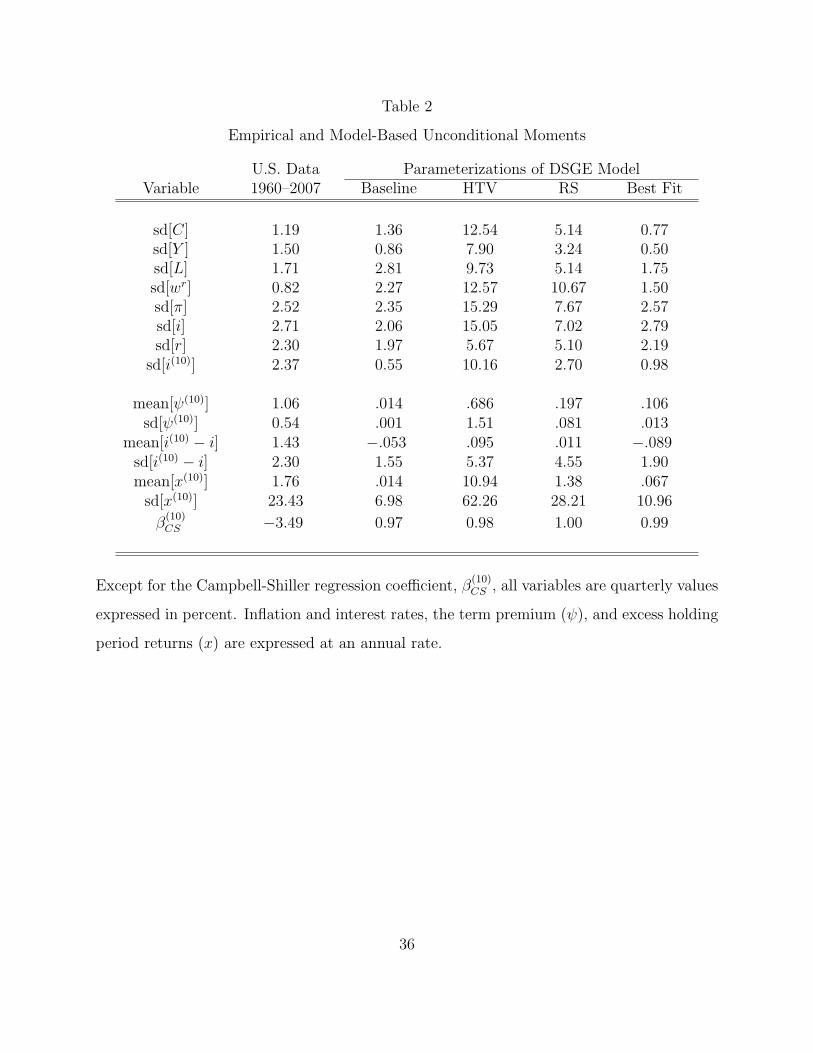
Table 2

Empirical and Model-Based Unconditional Moments

U.S. Data Parameterizations of DSGE ModelVariable 1960–2007 Baseline HTV RS Best Fit

sd[C] 1.19 1.36 12.54 5.14 0.77sd[Y ] 1.50 0.86 7.90 3.24 0.50sd[L] 1.71 2.81 9.73 5.14 1.75sd[wr] 0.82 2.27 12.57 10.67 1.50sd[π] 2.52 2.35 15.29 7.67 2.57sd[i] 2.71 2.06 15.05 7.02 2.79sd[r] 2.30 1.97 5.67 5.10 2.19

sd[i(10)] 2.37 0.55 10.16 2.70 0.98

mean[ψ(10)] 1.06 .014 .686 .197 .106sd[ψ(10)] 0.54 .001 1.51 .081 .013

mean[i(10) − i] 1.43 −.053 .095 .011 −.089sd[i(10) − i] 2.30 1.55 5.37 4.55 1.90mean[x(10)] 1.76 .014 10.94 1.38 .067

sd[x(10)] 23.43 6.98 62.26 28.21 10.96

β(10)CS −3.49 0.97 0.98 1.00 0.99

Except for the Campbell-Shiller regression coefficient, β(10)CS , all variables are quarterly values

expressed in percent. Inflation and interest rates, the term premium (ψ), and excess holding

period returns (x) are expressed at an annual rate.

36

Table 3

Unconditional Moments in Three Versions of the Benchmark DSGE Model

Campbell- C-C with C-C with quadraticCochrane quadratic adj. adj. costs to labor

Variable costs to labor and real wage rigidity

sd[C] 1.11 0.89 4.54sd[Y ] 0.71 0.59 2.86sd[L] 2.88 3.60 3.65sd[wr] 2.14 220.9 1.90sd[π] 2.25 19.7 5.98sd[i] 2.05 7.66 5.94sd[r] 1.96 21.4 2.81

sd[i(10)] 0.57 1.19 3.84

mean[ψ(10)] .027 .640 .168sd[ψ(10)] .001 .095 .001

mean[i(10) − i] −.035 .004 .004sd[i(10) − i] 1.56 6.52 2.43mean[x(10)] .033 .729 1.46

sd[x(10)] 7.23 23.03 23.52

β(10)CS 0.99 1.01 0.98

Except for the Campbell-Shiller regression coefficient, β(10)CS , all variables are quarterly values

expressed in percent. Inflation and interest rates, the term premium (ψ), and excess holding

period returns (x) are expressed at an annual rate.

37

0

50

100

150

200

250

300

350

400

0 0.5 1 1.5 2 2.5

Output cost of a 1 percent change in labor (in percent)

Mea

n te

rm p

rem

ium

(in

basi

s poi

nts)

Model with Campbell-Cochrane habit preferences

Baseline model

Fig. 1. Mean term premium in DSGE models with varying amounts of labor adjustment costs. The solid line shows the mean 10-year term premium in the baseline version of the benchmark model. The dashed line shows the mean term premium in the version of the model with Campbell-Cochrane habit preferences.