EXAMINING POVERTY AND INEQUALITY ACROSS SMALL …

Asia-Pacific Development Journal Vol. 18, No. 1, June 2011

125

EXAMINING POVERTY AND INEQUALITY ACROSS SMALLAREAS OF ISLAMIC REPUBLIC OF IRAN; TOOLMAKING

FOR EFFICIENT WELFARE POLICIES

Arman Bidarbakht Nia*

Small area estimation techniques are frequently used in poverty mapping.For this paper, an econometric approach to small area estimation, knownas the ELL method, was applied to estimate poverty and inequalityindicators in small areas1 of the Islamic Republic of Iran. This study aimsto determine patterns of poverty and inequality in small areas andhousehold characteristics related to them in order to provide practicaltools for a geographically targeted pro-poor policy. Drawbacks in thecurrent Government welfare policy (uniform cash distribution) along withthe diversity among provinces and small areas regarding scale of povertyand inequality and their correlates, as well as the level of living standards,underlines the need to utilize small area estimations as a tool forevidence-based policymaking.

JEL classification: G51, I32, I38.

Key words: Small area estimation, poverty, inequality.

I. INTRODUCTION

Small area estimation (SAE) methods are statistical techniques that borrowstrength from auxiliary information to estimate desired parameter(s) more preciselythan by direct estimation.2 The comprehensiveness of coverage of census data on

* Graduate School of Economics, Tokyo International University (TIU). The author is indebted toanonymous referees and the editor for their very helpful comments on earlier versions of this paper.Special thanks should be given to faculty of graduate school of economics at TIU for theirrecommendations and suggestions, in particular Professor Atsushi Maki. The author remains responsiblefor remaining errors.

1 For the purposes of this study, small areas are defined as urban and rural areas for each county.

2 A comprehensive review of the existing methodology on SAE and some recent developments on thetopic can be found in Rao (2003), Longford (2005) and Särndal (2007).


126

the one hand, and insufficient sample size in sub-domains in the household incomeand expenditure surveys on the other hand, prompted a research team from the WorldBank to introduce an econometric solution for the small area problem. Elbers,J. Lanjouw and P. Lanjouw (2002) proposed a method (called ELL) which combinesinformation from a household survey and a census to predict per capita expenditureas a measure of living standards for all households in the census dataset.

In this research, the ELL method has been applied to estimate poverty andinequality indicators in small areas in the Islamic Republic of Iran. The methodutilized micro-data from a household income and expenditure survey (HIES)conducted in 2007 combined with population and housing census 2006 dataset. Thediscrepancy in poverty and inequality among small areas is obvious from the results,with location being the most deterministic factor pertaining to poverty incidence. Thisstudy suggests that the existing strategy of uniform cash redistribution in the IslamicRepublic of Iran be replaced with a geographically targeted policy utilizing SAE. Aftertaking into account many household characteristics, location has a significantcorrelation with poverty and inequality. Although the lack of spatial informationprevents us from identifying the geographical features behind the impact of location,policymakers still need to take this into account and avoid uniform treatments fordifferent areas. On the other hand, comparing poverty lines reveals a large differencein living standards across regions (urban and rural areas of each province). Thediversity in poverty and inequality combined with the fact that the impact ofhousehold characteristics varies across regions could exacerbate the effects ofuniform redistribution policies on the household welfare.

No studies on poverty and inequality for small areas have been completed inthe Islamic Republic of Iran. The Government, through the Statistical Research andTraining Center, conducted two major studies in 2002 and 2003 on poverty but theirscope was limited to calculating only poverty lines and some other poverty indicatorsat the country level, in seven regions and for some occupation levels. Notably, twopredominant studies on poverty and inequality are Assadzadeh and Paul (2004) andSalehi-Isfahani (2009). The former evaluated changes in the extent of poverty in theIslamic Republic of Iran during the post Islamic period and the latter one examines thetrend of poverty and inequality in the three decades after the revolution. Assadzadehand Paul (2004) calculated poverty and inequality indicators not only for the countryas a whole, but also for nine geographic areas as well as for occupation levels.Based on the existing literature in the Islamic Republic of Iran, researchers in thecountry have been trying to estimate welfare indicators below the country level, butdue to limited sample size in small areas, the surveys mentioned above only cover theregions and some wide demographic groups. Nonetheless, ELL has been extensivelyimplemented in several countries in the last decades, including, among others, in


127

Cambodia (Fujii, 2007), Indonesia (Suryahadi and others, 2005), the Philippines(Haslett and Jones, 2005) and Viet Nam (Minot, Baulch, Epprecht, 2006).

The remainder of this paper is devoted to reviewing the methods used in theanalysis, to be introduced in section II, and evaluating poverty and inequality patternsusing small area estimations and poverty and inequality maps in section III. SectionIV contains policy implications based on the findings of the paper.

II. ESTIMATION METHODS

The ELL method is used mainly for poverty mapping for SAE. Recentlydeveloped by the World Bank, this method utilizes census information to predictwelfare measurements for households at the micro-level.

This section introduces the ELL method as well as the methodology used todetermine poverty and inequality correlates to compare and analyse these aspects ofwelfare in small areas.

ELL method

Consider yih as per capita expenditure of household h (h = 1, 2, ..., n

i) in area

i (i = 1, 2, ..., A) where ni is the number of sample units in area i and A is the total

number of small areas. The main concern is to fit an accurate predictive model of yih.

The following is a linear approximation to the conditional distribution of yih.

In yih = E [In y

ih | xT

ih] + u

ih = xT

ih β + u

ih(1)

where xih

is the vector of auxiliary variables (limiting to those that are commonto both survey and the latest census) for household h in the i th area and the vector ofdisturbances, u, follows distribution F (0, Σ). The x

ih includes both household and

area level variables to capture the effect of household and individual characteristicsas well as regional effects (tables A.1 and A.2 list these variables). Since thepredictive model (1) has been applied for each province separately, the variablesinvolved in x

ih vary across provinces. Thus, depending on the matching outcomes,

a subset of potential variables presented in the appendix is used for each province.The disturbance u

ih contains all the effects not described by auxiliary variables.

Although the area auxiliary information is involved in the xih, some unexplained effects

of area on the welfare will remain in the u. Therefore, allowing for area effects, thefollowing model is suggested for the disturbance term:


128

uih = η

i + ε

ih(2)

In model (2) ηi is area random effect, independent to ε

ih, and both are

uncorrelated to xih.

An initial estimate of β in equation (1) is obtained from the ordinary leastsquare (OLS) or weighted least squares (WLS) estimation and then û

ih denotes the

estimated values of disturbances. No heteroskedasticity for the area random effecthas been assumed, as many areas (672 in our case) are too small to causeheterogeneity. However, we allow for heteroskedasticity for variance of ε

ih. From this

error specification, one can also imply that the less the share of area effect in totalerror variance, the less one benefits from disaggregating data. From the followingdecomposition we can get the estimated values of η

i, ε

ih and also variance of ε

ih:

ûih = û

i. + (û

ih – û

i. ) = η

i + e

ih(3)

Where ûi.

is the mean of estimated disturbances, ûih, over households in the area i

which estimates ηi, and e

ih = û

ih – û

i. estimates ε

ih. Elbers and others (2002) proposed

a logistic form for variance of εih

to avoid negative or extremely high predictedvariances,

In = zTih α + r

ih or e2

ih = ,

in which A and B are upper and lower bounds to avoid extreme values for thevariance and z

ih is a vector of household characteristics which is not necessarily

different from xih. These bounds can be estimated simultaneously with parameter α.

However, Elbers and others (2002) found that using measures B = 0 and A = 1.05 xmax (e2

ih) leads to similar estimates of model parameters which are more practical.

This logistic form also does not allow for negative values of variance.

The variance estimator for εih

can be achieved as follow by using the deltamethod (Greene, 2007).

σ 2εih = + — vâr (r) (4)

The other component of variance is variance of area random effects, σ2η

, which isestimated using moment conditions (Elbers and others, 2002).

After estimating variance of error terms, σ2εih

and σ2εih

, generalized leastsquare (GLS) estimates of model parameters, β

GLS, have been obtained by applying

estimated variance covariance matrix Σ. Sampling weights are incorporated in allsteps in the model estimation.

ˆ

12

ˆ

ˆ

[ ] [ ]

[ ] [ ]AB1 + B

ˆ

AB (1 – B)

(1 + B)3

AezTih

α + rih + B

1 + ezTih

α + rih

e2ih – B

A – e2ih

ˆˆ


129

At this point, the estimated error terms, ηi and e

ihare simulated, either by

assuming proper distributional form for them or using their empirical distributions.Simulation allows us to estimate welfare indicators (introduced later in this section) aswell as their sampling errors. The ELL method uses bootstrapping to simulate welfareestimators. In this method, we repeatedly draw samples with replacement randomlyfrom the error terms’ empirical distribution or from suitable distributions (normal ort-student with proper degrees of freedom). Then the welfare indicator for the smallarea i, W

i, can be estimated as

Wi =

where Wir

is the simulated welfare indicator in i the small area and R is the number ofiterations. The variance of welfare estimates can simply be estimated as follows:

Var(Wi) = — Σ (Wir

– Wi) 2 (6)

Practical aspects

This section clarifies some important aspects of the econometric model andillustrates the method with which we can derive explanatory variables that are asaccurate as possible to ensure that all the potential of the census information isutilized to predict the household’s per capita expenditure precisely. The mainpurpose of this practice is to choose explanatory variables that are proxy indicators ofa household’s consumption and have strong logical and empirical links to that. Oneadvice would be to identify all possible main determinants, including, among others,household size, the age and gender composition of the household, education, health,social capital and assets, and leave the effects of other factors that operate at higherlevels to be captured by the area random effect. To ensure that all aspects ofconsumption expenditure are considered and household information is used in themost efficient way, a comprehensive list of potential proxy indicators (explanatoryvariables) which meet some eligibility conditions (their wording and response optionsin the questionnaire, reference periods, concepts and distributions, which all haveto be same for both survey and census) has been identified for entry into theeconometric model. Therefore, all these criteria have been tested beforehand andonly variables that met these three conditions were identified as candidates as proxyindicators. The two most important considerations are the following:

• The linkage between census and HIES is rather tenuous because ofthe differing context of the two data collection processes. Thewording and format of the questions have been checked to ensure

ˆ

~ Σ Wir

R

r = 1

ˆ

R

ˆ

R

r = 1

1R

ˆ~ ~


130

that the difference in wording or response options do not generateconceptual inconsistencies and in case of disagreements, possiblechanges were made to resolve them. Typical examples are joboccupation and head of collective households.

• A particular question must measure the same feature and provide thesame range of information in both systems. Probable differencesbetween the two systems regarding concept, referenced period orsubpopulation covered by the question should be carefully taken intoaccount. For instance, the distinction between agriculture andnon-agriculture occupations has different criteria in two systems. Inorder to have consistency between census and survey, the joboccupation in HIES has been redefined using International StandardIndustrial Classification (ISIC) codes.

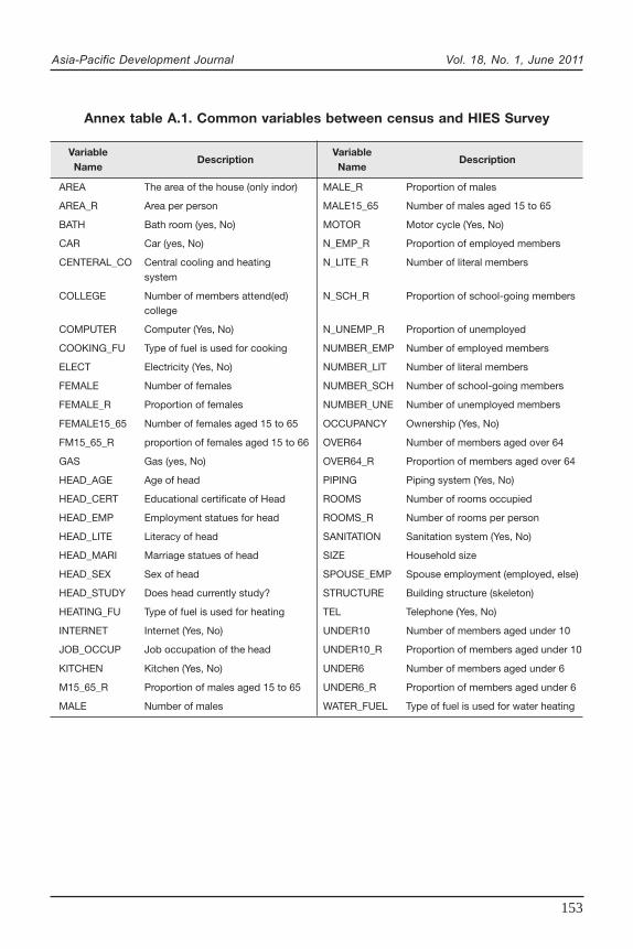
Annex table A.1 shows the final list of potential variables after taking intoaccount the requirements and adjusting some questions, such as recoding, collapsingresponse options and redefining subpopulations.

In order to achieve household variables, the initial variables need to bechecked to make sure that the distribution is the same in the survey and census.There are several methods to test the distributions depending on the type of the data.However, these statistical tests are sometimes very strict and we may lose all thepotential variables using these criteria. Therefore, it suffices to test for equality of themeans of the continuous and the proportion of the categorical variables. Thevariables with statistically equal means (proportions) in both the census and thesurvey have been determined as matched variables for every province separately andapplied in the corresponding predictive model. Therefore, among the provinces, theremay be different sets of matched variables.

To take into account the area effect, an area level vector of independentvariables should be introduced into the consumption model. In contrast to thehousehold variables, for this part, only census aggregate information in the area levelcan be used. This enables us to also benefit from variables that have not beenequally distributed in the survey and the census. For example, household size hasdifferent means in the survey and the census in rural areas but for this part, averagehousehold size for each area as an independent variable can be used. The sameapplies to availability of gas, telephones, car or sanitation systems, which areanticipated to influence the household welfare level. The area level independentvariables are listed in annex table A.2.


131

An important consideration about the model is that it is estimated only forpredictive purposes, and it would not be appropriate for concluding any cause-effectrelationships between household expenditure (income) and the proxy indicators.Therefore, the magnitude and signs of the coefficients are not important in suchpredictive models. What matters here is the level of correlation, or the R-squaredvalue of the regression of lny on X. In fact, this econometric model is designed tocapture the association between expenditure and some proxy variables, and to returna prediction as accurate as possible. Nevertheless, it does not mean that thestatistical significance of the coefficients is not a consideration. Indeed, it isimportant to select proxy indicators that will lead to a model with an R-squared valueas close to 1 as possible while having all coefficients statistically significant.

Poverty lines

To measure poverty indicators in a society, it is necessary to have a thresholdof access to goods and services under which individuals are classified as poor.Poverty line is a monetary cost to a given person, at a given place and time, ofa reference level of welfare (Ravallion, 1998).

Poverty studies on the Islamic Republic of Iran have used different measuresof poverty lines due to either conceptual or technical differences. However all ofstudies were taken at the country level or ultimately cover geographical regions oroccupational categories. As this study analyses welfare in small areas, using suchcountry-wide poverty lines demands a very restrictive assumption on tastes, livingstandards and markets. On the other hand, the HIES sampling design allows forestimation of poverty line in each region (urban and rural areas for each province).Following Ravallion (1998) with slight modifications, particularly correcting for outliersof average cost of one kilocalorie (Kcal) per person, a poverty line has been estimatedfor every region based on cost of basic needs (CBN). The CBN poverty line has twocomponents, food and non-food. The following is short description of estimationprocess for the CBN method.3

Food component

A critical issue regarding the food component is the minimum nutritionalrequirement for an individual. Although international institutes, such as the WorldBank, suggest 2,100 Kcal per person per day, not all countries use that figure as thestandard criterion. In fact, the Islamic Republic of Iran does not seem to have an

3 For more detailed review of this, please refer to Ravallion (1994, 1998).


132

official criterion for this.4 To keep comparability with other studies and to stay close tointernational standards, 2,200 Kcal was used for this study as the minimum nutritionalrequirement for good health.

To compute the minimum cost of the caloric requirement, a reference groupmust be selected. As the demand patterns are unknown in the regions, one methodis to use a nationally fixed group, poorest 30 per cent in this case, and set a bundle ofgoods for each region from the individuals who belong to this national referencegroup. After finding the average calorie cost per person in each region, food povertyline is LF

i = C

i x 2,200 per person per year in region i in which C

i is the average calorie

cost per person per year in the reference group of the i th region.

Non-food component

The welfare consistency and time and location matters are more significantwhen it comes to the non-food poverty line. Ravallion (1994) suggested upper andlower bounds for non-food component of poverty line. The upper bound is the meanper capita per year non-food expenditure for households whose food spending equalsthe food poverty line. The lower bound is the mean per capita per year non-foodexpenditure for households whose total expenditure equals food poverty line. Thenthe following is defined:

Upper line in region i : LUi =

Lower line in region i : LLi = LF

i x (2 – S

i )

Si : Average food-share in the corresponding reference group in region i.

in which LF, LU and LL are the food component of the poverty line and the upperand lower bounds for the non-food component, respectively. A conservative povertyline for region i is the average line given by the arithmetic mean of upper and lower

lines; Li = .

4 To the best of my knowledge, at least five measures have been used in previous studies. 2,197 and2,300 (Statistical Center of Iran, 2004), 2,200 (Management and Planning Organization, 2000), 2,168(Pajooyan, 1994), 2,500 (Akhavi, 1996). The author’s calculations, however, indicate that the minimumrequirement should be 2,448 Kcal according to the table of the daily minimum caloric requirementadjusted for age distribution in 2006 housing and population census.

LFi

Si

LLi + LU

i

2


133

Annex table A.3 shows the regional poverty lines as well as the national levellines for rural and urban areas. One may question that sample sizes are not largeenough in each province to estimate precise poverty lines.5 However, through theapplication of the bootstrap method with 1,000 replication, the coefficient of variation(CV) for poverty lines in all 60 regions have been estimated. The CVs vary in therange of 1 to 6 per cent, which is quite reasonable.

A comparison between the regions by their poverty lines may be misleading.As these poverty lines are absolute in terms of living standards and in this case thehousehold consumption is the living standard indicator, differences between povertylines arise from several factors which affect average household expenditures ina particular region, such as public goods availability, living standards, consumers’taste, household wealth, price levels and relative prices and natural endowments.The reference groups for the non-food component provide different functions forupper and lower poverty lines. Depending on the case, any of the poverty linescan be used in welfare policies. For instance, in minimum wage determination,a government may decide to use the upper poverty line, but in the case of foodsubsidies, the lower poverty line would be a better criterion to distinguish householdsthat are unable to meet the minimum quantity of food intake after spending on verybasic non-food commodities. The average poverty line is a conservative line to bereported as official statistics and suitable for policy evaluation and countrywidecomparisons. In this study, the average poverty lines are used for small areaestimations in each province.

Poverty and inequality correlates

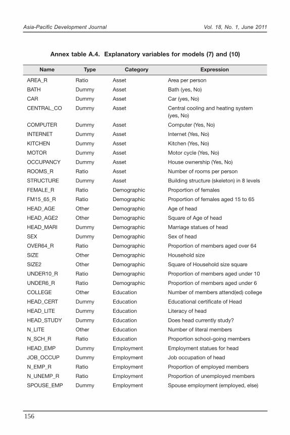
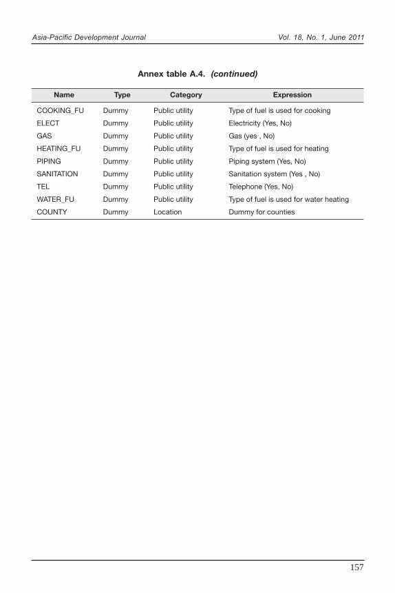
In addition to the regional pattern and the disparity of poverty and inequality,an informed welfare policy requires information on attendant correlates of the welfareindicators. A regression-based inequality decomposition method (Fields, 2003) hasbeen used to find the contribution of each explanatory variable and consequently,each category of variables in per capita expenditure’s variation. A logistic regressionhas been applied to find influential factors on the likelihood of being poor. Obviously,provincial poverty lines have to be used for the latter one to distinguish the poor fromthe non-poor. The same explanatory variables have been included in the two models.Annex table A.4 presents explanatory variables of models (7) and (10). In addition tothe variables in annex table A.4, location dummies have been introduced into themodel to capture the regional effects. Although the regional effects are not veryinformative without doing spatial analysis, the magnitude of the effects is stimulus forfurther deep analysis on regional differences and also for policy implication purposes.

5 The HIES sample sizes vary in the range of 480 to 1,700 households across small areas.


134

Inequality decomposition

It is a very common practice in poverty studies to fit a semi-log regressionmodel to generate per capita income (consumption expenditure) using explanatoryvariables found by either past experiences or according to the theory. Fields (2001,2003) used this income-generating model to decompose income inequality not onlyfor one single model but also to find the contribution of explanatory variables in theinequality changes between two groups or times. This paper only addresses theformer objective and uses the regression-based inequality decomposition method tofind the share of per capita expenditure inequality which is attributable to eachexplanatory variable and each group of variables.

Below is an example of a similar model with equation (1), but without thecomplicated error specifications.

In y = Xβ + u (7)

Where y and X are a vector of per capita consumption expenditure and a matrix ofexplanatory variables, respectively. u is the error vector and β is the vector of modelparameters to be estimated. The rirst column of the explanatory variables matrix, X,always accounts for the intercept. Therefore, X is in the dimension of n x (K + 1) inwhich K is number of explanatory variables and n number of households. Thecontribution of k th explanatory variable is given by equation (8).

SK = (8)

where βk is the OLS estimation of corresponding model parameter for k th variable, x

k

is the k th explanatory variable and σ 2In y

is the variance of. The sK

can be interpretedas the share of explanatory variable x

k in the total variation of logarithm of per capita

expenditure. It is clear from equation (8) that the contribution of the intercept in the

expenditure variation is zero.6 The important identity of sk is that Σ S

k = R2 and

sequentially Su = 1 – Σ S

k . Therefore, the percentage contribution of th variable in

the R-square can be calculated as:

βk cov (x

k, In y)

σ 2In y

ˆ

6 Morduch and Sicular (2002) disputed this decomposition method, first proposed by Fields (1998), forzero contribution of constant term due to log functional form. Nonetheless, in the Morduch and Sicular(2002) proposed model neither can derive the contribution of intercept and error term from the natural ruleof decomposition, whereas a large share of expenditure variation is left unexplained in the proposedfunctional form. For a general approach to the inequality decomposition refer to Wan (2004).

K

k = 1K

k = 1

ˆ


135

Pk = x 100

In other words Pk is the share of k th variable in the model predictability.

In practice, there are different types of explanatory variables in matrix X. Forcontinuous variables, only one s

k exists, but in the case of categorical variables, the

contribution of each variable equals the total of all sk’s for corresponding dummies in

the model. Also, for each category of variables, such as demography or assets, thecontribution coefficient is again simply the total of all s

k’s in the category.

Poverty correlates

Logistic regression analysis is often used to investigate the relationshipbetween discrete responses and a set of explanatory variables. For binary responsemodels, the response of a sampling unit may or may not take a specified value (in thiscase, per capita expenditure may or may not be under the poverty line). Suppose x isa row vector of explanatory variables and π is the response probability (probability ofbeing poor) to be modeled. The linear logistic model would then have the followingform:

log it (π ) = log ( ) = α + xβ (10)

in which α is the intercept parameter and β is the vector of the slope parameters. Theleft-hand side of this equation is called the log odds ratio. Obviously, provincialpoverty lines have been used to construct the response variable.7

Poverty and inequality indices

Among the numerous articles on poverty and inequality measures, one of themost widely used sources is Fields (2001), which covers a wide range of poverty andinequality indicators. For this study, the most popular indices have been applied tocompare both poverty and inequality among small areas.

A class of poverty measures identified by Foster, Greer, and Thorbecke(1984) known as FGT measures can be expressed as follows:

Pα = Σ wi ( )α (y

i < z, W = Σ wi

) (11)

sk

R2

7 A maximum likelihood estimation of parameters can be computed by using computer programs,which are relatively inexpensive. The reader may refer to Maddala (2001) for more technical details.

π1 – π

1W

np

i = 1 zz – y

i

i


136

where z is the poverty line, yi is expenditure for i th poor individual, n

p number of poor

individuals and wi is the sampling weight for i th sampling unit.

The different values of α in equation (11) give different measures of poverty.Poverty incidence, the proportion of the population whose annual per capita incomefalls below annual per capita poverty threshold level is derived when α = 0. Thismeasure is referred to as the poverty head count ratio. The depth of poverty (or thepoverty gap) is derived when α = 1. P

1 takes into account not only how many people

are poor but how poor they are on average. If we rearrange the formula (11) for P1, it

is equal to the head count ratio (P0

) multiplied by the average percentage gapbetween the poverty line and the income (expenditure) of the poor. When α = 2, thisequation gives a measure known as severity of poverty (or squared poverty gap). P

2takes into account not only how many people are poor and how poor they are butalso the degree of income inequality among poor households. It is equal to theincidence of poverty (P

0) multiplied by the average squared percentage gap between

the poverty line and the income of the poor.

Inequality measures show the degree of the discrepancy among individualsin terms of their income (expenditure). The Gini coefficient is the most commonlyused inequality measure in the literature. Equation (12) shows a weighted form of theGini index,8

Gini = + Σ wi y

i [ρi

+ 0.5 (wi – 1)] (12)

ρi = ρ

i-1 + w

i-1 (i > 1), ρ

1 = 1

in which y is the average per capita expenditure in the region. In fact, the Ginicoefficient is the area above the Lorenz curve and below the diagonal 45-degree linedivided by the area under the diagonal line.

III. NUMERICAL RESULTS

An extensive number of estimates has been produced by using the above-mentioned techniques, making comparisons and interpretations difficult. To preventconfusion, this report does not focus on detailed estimations over small areas butinstead concentrates on some extreme cases. Maps are very instrumental tools tovisually compare different areas and diagnosing the patterns and disparities of

8 The reader may refer to Deaton (1997) for more details.

W + 1W – 1

2

W (W –1)y– i

–


137

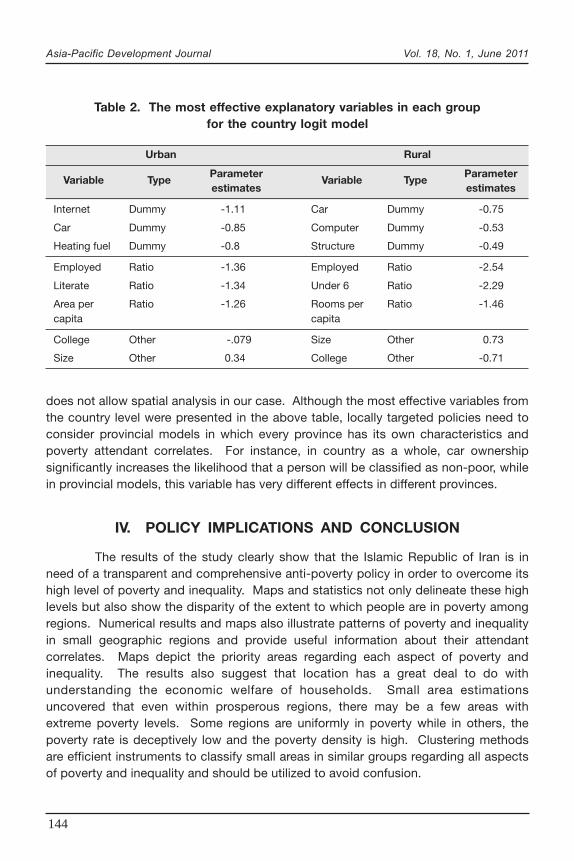
indicators over the country.9 Annex figure A.1 shows the location and names ofprovinces.

National and regional poverty and inequality

The results indicate that the national headcount poverty rate (P0) in rural

areas (15 per cent) is significantly higher than in urban areas (11 per cent). This gap iseven wider when comparing the depth of poverty (P

1). The national level in rural areas

is 0.04 compared to 0.029 in urban areas. As for the severity of poverty, the (P1)

indicator, in which the distribution of the expenditure is rated in addition to thepoverty gap, the figure is 50 per cent higher in rural areas at 0.018 versus 0.012 inurban areas.

For the study, the Gini index was used to measure inequality in terms of percapita consumption expenditure. Even though poverty incidence is higher in ruralareas, the results show that income (expenditure) is distributed more equally in ruralareas than in urban areas. This is due to homogeneity of living standards among ruralhouseholds.

At the regional level, the rankings of urban and rural areas in terms of P0 by

province tend to vary. This is not the case, however, for province 11 (Sistãn vaBaluchestãn), ranked as the poorest province in both its urban and rural areas andprovince 02 (Mãzandarãn), ranked as the second richest province in both areas. Thelargest gap between urban and rural areas in terms of poverty incidence has beendetected in provinces 23 (Tehrãn) and 15 (Lorestãn). In these two provinces, thepeople in the rural areas are much poorer than those in urban areas (more than twice).Annex table A.5 shows national and regional estimates of poverty and inequality.

Poverty and inequality in small areas

The Islamic Republic of Iran consists of 336 counties. To account for theurban and rural areas in each county, welfare indicators have been estimated in672 small areas which range in population from 781 to 7,872,280. This level ofdisaggregation is very informative for pro-poor policies since it provides keyinformation for studying patterns in poverty and inequality and their relationships withother characteristics of small areas.

9 Detailed statistics on the small area estimations are presented in Bidarbakht-Nia (2009) and are alsoavailable from the author upon request.


138

Poverty and inequality in rural areas

A comparison of the estimates of the regional level with those of the smallareas indicates that using only regionally disaggregated information in policymaking isunreliable. Although province 01 (Gilãn), for example, has a relatively low rate ofpoverty and inequality, there is considerable diversity in all of the indicators amongthe counties in the province. In province 05, (Kermãnshãh), the discrepancy is widewith regards to expenditure inequality and in provinces 06 (Khuzestãn), 08 (Kermãn),10 (Esfahãn) and 27 (Golestãn), only the poverty indicators vary within each province.In province 00 (Markazi), most of the counties fall in the first quintile (poorest 20 percent) and in 03 (East Ajarbãijãn), all counties fall in the last quintile of inequality (20per cent highest inequality). In province 06 (Khuzestãn), most of the counties havehigh poverty and low inequality. In provinces 18 (Bushehr), 26 (Ghazvin), 24 (Ardebil)and 02 (Mãzandarãn), all of their counties are relatively better off when compared withprovinces 11 (Sistãn va Baluchestãn) and 21 (Yazd) in which almost all of theircounties suffer from high poverty and inequality. Kohrang and Ardal are the onlycounties in 14 (Chãharmahãl va Bakhtiãri) that suffer from a high poverty rate.

As extreme cases, Savãd-Kuh, Jam and Tonekabon have the lowest povertyrate (less than 3 per cent) and Irãnshahr, Sarbãz and Shãdegãn have the highestpoverty rate (more than 47 per cent). Of note, all the counties in the 11 (Sistãn vaBaluchestãn) fall in the last quintile in terms of poverty but vary among quintiles interms of inequality.

Poverty and inequality in urban areas

As for the rural areas, diversity among counties inside the provinces isobvious in some cases. Poverty indicators in provinces 27 (Golestãn), 14(Chãharmahãl va Bakhtiãri), 17 (Kohgiluyeh va Boyrahmad) and 23 (Tehrãn) varywidely among their small areas. In province 08 (Kermãn), the county Bam, is anexception as its poverty incidence and inequality (poverty rate 6 per cent and Giniindex 0.37) are both relatively low. This is due to the reconstruction activities and aidtied to the 2003 earthquake in this area. In province 23 (Tehrãn), the characteristics ofthe capital city, also called Tehrãn, is a totally different than what is found in thecounties. Tehrãn enjoys a low poverty rate compared with other counties in theprovince but its Gini coefficients are almost the same, with the exception of somesmall counties in which inequality is not surprisingly very low due to similaritiesbetween households. Province 21 (Yazd), 22 (Hormozgãn) and 29 (South Khorasãn)have high levels of poverty and inequality in almost all their counties. In (13)Hamedãn, most of the areas have high inequality but low poverty rates. In 11 (Sistãnva Baluchestãn), a majority of its counties have poverty rates between 30 per cent


139

and 62 per cent. Two counties in the province that are an exception to this are Zahakand Konãrak, which have very low poverty and inequality levels.

In province 06 (Khuzestãn), half of its counties are in the last quintile (poorest20 per cent) with respect to the poverty rate despite the fact that the province hasa lot of industry, including oil production, contributes a share of 15.4 per cent to thecountry’s GDP (the second highest share after Tehrãn) and has the second highest percapita GDP after province 17 (Kohgiluyeh va Boyrahmad). This shows that there isa gap between production value added (or GDP) and disposable income. Althoughper capita GDP mainly represents the productivity of the people in one region, it is nota good proxy for income in regional studies. This is because the central governmenttends to control the reallocation of the budget and one of the factors for determininghow the funds are distributed is based on the political power of local governments,which often takes precedence over regional GDP. Surprisingly, inequality is relativelylow in this province (mostly around 0.35).

The least poor small urban areas (with a poverty rate of less than3 per cent) are Jam, Bushehr, Gilãngharb, Bijãr, Nowshahr, Ghasr-e-Shirin, Tonekãbonand Marivãn. In contrast, Sarbãz, Sarãvãn, Kalãt, Bahme’ei and Khavãf have thehighest level of poverty incidence (more than 47 per cent).

In summary, the estimated poverty rate is less than 0.10 in 31 per cent of therural counties and more than 0.20 in almost 29 per cent of counties. These statisticsare correspondingly 36 per cent and 26 per cent for urban counties which shows thatmore rural areas are in poverty (in terms of proportion) than urban areas.

Mapping poverty and inequality

Poverty mapping methods have been utilized to visually investigate patternsin welfare indicators in the country. The incidence of poverty in urban areas is shownin annex figures A.2 and A.3. A comparison between two figures shows that thepoverty rate varies widely within one province and that the scale of discrepancy isvery different among provinces. For example, in provinces 09 (Khorãsan Razavi) and11 (Sistãn va Baluchestãn), poverty rates among counties range between less than6 per cent and more than 60 per cent, while in provinces 04 (West Azerbãijãn),18 (Bushehr), 12 (Kordestãn), 05 (Kermãnshãh) and 02 (Mãzandarãn), the rates differbetween 1 per cent and 15 per cent. Generally speaking, in the north-central andnorth-western parts of the country, there is homogeneity among the interior areas,while in the eastern and south-western regions, the provinces are heterogeneous andgenerally have higher rates of poverty. In terms of climate circumstances, with theexception of 18 (Bushehr) and 29 (South Khorãsãn), the provinces under study withfavourable weather conditions, have relatively low poverty levels in their urban areas.


140

Some may assume that this is tied to productive agricultural activities but it couldeasily be tied to other income-generating factors, such as tourism and access to theforeign market (either legal or illegal). In the case of province 18 (Bushehr), the lowlevel of poverty may be attributed to income generated from a special economic zoneset up there that enables access to foreign markets through the Persian Gulf.Nevertheless, the information available is not definitive and can only serve as guide indetermining the patterns and the magnitude of the effects of some explanatoryvariables. More information is needed to ascertain the spatial differences and theirdeterminants. Annex figures A.4 and A.5 illustrate rural poverty rates in provinces andsmall areas, respectively. Similar to the urban case, the disparity in some provinces isconsiderable in rural areas. The pattern of poverty in rural areas in the north-westernpart of the country is quite different from its urban counterparts. The urban areas arebetter off than the rural areas, with the exception of the borderline areas in thenorthern part of this region where the economy benefits from access to foreignmarkets and productive agricultural activities.

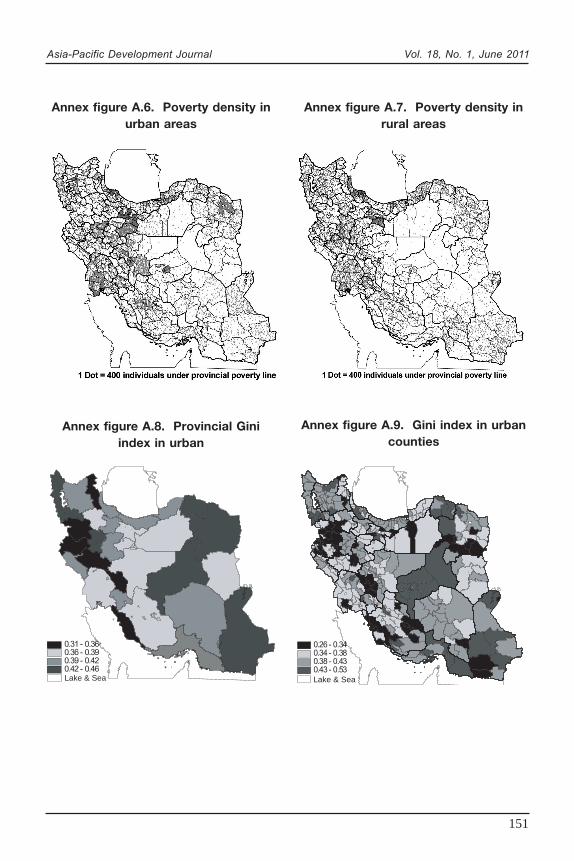
Another way to determine patterns of poverty is to estimate the number ofpeople whose income is under the poverty line in each small area (poverty density).Poverty density for each area is estimated by multiplying the corresponding povertyrate times the population. Annex figures A.6 and A.7 depict poverty densities forurban and rural areas, respectively. In these maps, each dot represents 400individuals living under the provincial poverty line. Notably, in both urban and ruralareas, regions with high levels of poverty tend to have low poverty density. Anexception to this is the south-east region. As poor areas are mainly located in theeastern part of the country, which, except for the extreme north-east, has a desertclimate and is less populated than other regions. Generally speaking, many areaswith low level of poverty incidence, which may not be considered as a priority inpro-poor policies, have high density of poverty. Therefore, it must be noted thatrelying only on the poverty rate may cause exclusion of the majority of the poorpeople in the country. To avoid this, it is very helpful to carefully examine all povertyand inequality indicators simultaneously for areas. Since none of the existing povertyindicators contributes poverty density in the formula it is more likely to be ignored. Acomparison of the maps on poverty rate and poverty density shows that in someprovinces, such as 06 (Khuzestãn), 25 (Ghom), and in some areas in 11 (Sistãn vaBaluchestãn), there is a high level of poverty not only in terms of percentage but alsoregarding population in poverty. Consequently, multivariable clustering is required toput similar counties in the same category (discussed later in this section).

A comparison between rural and urban areas regarding their inequality Giniindex (annex figures A.8 – A.11) for the country as a whole illustrates that the generallevel of inequality in rural areas is lower than in urban areas. This can attributed to the


141

narrower differences in living standards among rural households. Despite thediversity in poverty, inequality is homogeneous across the country. As discussed indetail later in this study, location is the main explanatory variable for povertyincidence. On the other hand, household characteristics have more of an effect onthe level of inequality than location effects.

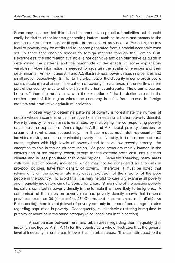
Finally, to assist in setting priorities for policymaking, small areas have beenclustered based on the poverty and inequality indicators (three FGT indicators, theGini coefficient and poverty density) utilizing a fuzzy clustering technique. Small areasin each cluster are similar regarding to all of their poverty and inequality indicators.10

Table 1 shows the cluster means of poverty and inequality indicators. In this table,small areas in cluster 1 can be considered non-poor on average, based on allindicators, and sequentially clusters 2 and 3 are worse off except in the case of Ginicoefficient in rural areas.

Table 1. Cluster means of welfare indicators

Cluster* P0 P1 P2 GINI Poverty Density

Urban 1 0.08 0.02 0.005 0.37 5 808

2 0.14 0.03 0.012 0.39 13 342

3 0.24 0.07 0.028 0.41 27 978

Rural 1 0.09 0.02 0.007 0.34 4 682

2 0.16 0.04 0.015 0.39 8 348

3 0.26 0.07 0.029 0.37 19 493

* Number of clusters (3) is arbitrarily determined.

10 For more detail explanations about fuzzy clustering, please refer to Bezdek (1980).

This classification does not mean that, for example, every small area incluster 1 has a lower poverty incidence than small areas in other clusters. Detailedinformation shows that there might be small areas with one or more relatively highwelfare indicators in cluster 1. This is because the membership function for eachsmall area is a multivariate function in which all the indicators are simultaneouslyconsidered. Annex figures A.12 and A.13 map the clustered small areas.

Poverty and inequality correlates

The evaluations outlined in previous sections indicate that the patterns ofpoverty and inequality vary greatly across the country and between urban and ruralareas. Policies aimed at mitigating household deprivations need to be informed with


142

disaggregated statistics that visually illustrate areas and subpopulations with highpriorities regarding poverty and inequality. Nevertheless, at this point, two importantquestions remain unanswered; “what characteristics explain the inequality?” and“who is more likely to be poor?” This study does not assume that there is causalityrelationship between poverty and inequality and household characteristics. Instead, itdetermines what factors explain inequality and are more closely related to thelikelihood of being poor. To show the general effect of explanatory variables onpoverty and inequality, the country level models (for rural and urban separately) havebeen fitted. Moreover, a linear logistic model has been estimated separately for eachprovince in order to monitor different effects of explanatory variables on povertyacross regions. Regarding to the inequality decomposition, the contribution of eachexplanatory variable (S

k) and, to be more precise, the share of each variable in the

R-square (Pk) have been calculated for the national level.11 Bar charts in figure 1 show

the percentage share of each category in the predictability of the country-level model.In other words, it indicates the overall effect of each group of explanatory variables onthe expenditure distribution in country level. The asset category is the most influentialfactor in both urban and rural with almost half of the contribution in the per capitaexpenditure variation. In both rural and urban areas, education level and location aretwo other effective categories with the difference being that location has much greatereffect in rural areas than in urban areas. This may be attributed to the many spatialcharacteristics which could affect the income level and income inequality in ruralareas, such as transportation facilities, natural endowments and distances to the bigcities. As location is an exogenous variable, this result suggests that investing ininfrastructure in rural areas could mitigate inequality. However, to determine this,more Geographical Information Systems (GIS) information is required to analyse thespatial determinants of the poverty and inequality. Inside categories, the mosteffective variables are car ownership and the floor area per person in the asset groupfor both urban and rural areas. In the case of demographic the size of household hasthe most influence on the per capita expenditure disparity.

The interpretation of coefficients in the logit model is not straightforward andusually requires some extra work after parameter estimations have been made. Inthis paper, the explanatory variables (annex table A.4) are divided into three groupsaccording to their measurement scale: dummy variables, ratios and other types(continuous or counts). The coefficients are interpreted as the amount of change inlog odds due to a one unit increase in explanatory variables. Thus, absolute values ofthe coefficients are comparable in each category; the corresponding explanatory

11 Since semi-logarithmic functional form applied to inequality decomposition is not mean-independent,only a country model has been fitted for inequality decomposition.


143

Figure 1. Percentage contribution of each category of variables in theR-square of expenditure model

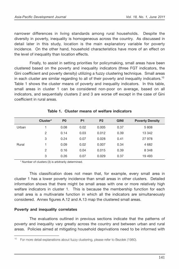
variable becomes more effective as the absolute value of the coefficient increases.The logit model has been applied at the country and the provincial levels in both ruraland urban areas. Table 2 illustrates the most effective variables in country model.Note that location dummy variables (336-1 dummies for counties’ effects in themodel) have been excluded from the comparison.

However, when the location parameter estimation is included, it can beobserved that in the dummy group, about 90 per cent of location effects (eitherpositive or negative effects depending on the degree of poverty) in urban areas and60 per cent in rural areas are significant and more influential than other dummyvariables. Location effects are more informative when using provincial models forgeographically targeted pro-poor policies. The regional results (not presented here)indicated that in almost every province location is highly correlated with povertylikelihood. These results only show the degree of importance of location whenanalysing poverty. However, information available cannot explain why location is sucha determinant factor. Lack of GIS information in the Islamic Republic of Iran, such asdistance to the markets (domestic and foreign) and facilities, soil fertility and climate

41

16

11

3

8

21

47

17

12

2

6

17

0

20

40

60

Asset

Dem

ogra

phic

Educa

tion

Employ

men

t

Public

Utility

Loca

tion

Urban Rural

Per cent


144

does not allow spatial analysis in our case. Although the most effective variables fromthe country level were presented in the above table, locally targeted policies need toconsider provincial models in which every province has its own characteristics andpoverty attendant correlates. For instance, in country as a whole, car ownershipsignificantly increases the likelihood that a person will be classified as non-poor, whilein provincial models, this variable has very different effects in different provinces.

IV. POLICY IMPLICATIONS AND CONCLUSION

The results of the study clearly show that the Islamic Republic of Iran is inneed of a transparent and comprehensive anti-poverty policy in order to overcome itshigh level of poverty and inequality. Maps and statistics not only delineate these highlevels but also show the disparity of the extent to which people are in poverty amongregions. Numerical results and maps also illustrate patterns of poverty and inequalityin small geographic regions and provide useful information about their attendantcorrelates. Maps depict the priority areas regarding each aspect of poverty andinequality. The results also suggest that location has a great deal to do withunderstanding the economic welfare of households. Small area estimationsuncovered that even within prosperous regions, there may be a few areas withextreme poverty levels. Some regions are uniformly in poverty while in others, thepoverty rate is deceptively low and the poverty density is high. Clustering methodsare efficient instruments to classify small areas in similar groups regarding all aspectsof poverty and inequality and should be utilized to avoid confusion.

Table 2. The most effective explanatory variables in each groupfor the country logit model

Urban Rural

Variable TypeParameter

Variable TypeParameter

estimates estimates

Internet Dummy -1.11 Car Dummy -0.75

Car Dummy -0.85 Computer Dummy -0.53

Heating fuel Dummy -0.8 Structure Dummy -0.49

Employed Ratio -1.36 Employed Ratio -2.54

Literate Ratio -1.34 Under 6 Ratio -2.29

Area per Ratio -1.26 Rooms per Ratio -1.46capita capita

College Other -.079 Size Other 0.73

Size Other 0.34 College Other -0.71


145

Small area estimations of poverty gap are very helpful for estimating theminimum budget required for eliminating poverty in particular region. This enablesgovernments to avoid extreme payments during budget allocation. Table 3 shows thebudget required to raise all members of the population above the correspondingpoverty line using estimates of poverty gap in different levels of disaggregation.The difference between two budget requirements is a measure of efficiency thatgovernment can gain from small area estimations. Applying an informed welfarepolicy with small area estimations and saving 27 per cent of budget, governmentcan take the opportunity to spend a significant share of the subsidy revenue ondevelopment programmes according to the regional requirement.

Table 3. Required budget for eliminating poverty

Level Required budget* (USD billion)

County 1.00

Province 1.37

* Required budget to raise every one above poverty line = poverty gap xpoverty line x population

The discussion in this paper suggests that small area estimations arebeneficial for setting a geographically targeted pro-poor policy. Although the resultsdo not indicate which geographical factors affect economic welfare, a spatial analysisusing detailed GIS information can be applied to obtain additional input ascomplementary information for policy implications. Reallocating a budget based onregional requirements not only alleviates poverty and inequality but also creates jobsand boosts production and income, which consequently raises living standards. Forinstance, geographical factors in rural areas, which cannot be addressed by currentpolicy, may be insufficient educational facilities, an inefficient health care system andlimited infrastructure. One reason behind this is that government has no control onintrahousehold allocations and usually in poor households, the allowance received byhead of household is not spent on education, health and other needs of children. Incontrast, in a growth-oriented policy, the government takes into account regionalfactors and household characteristics, and invests more efficiently. As a result,governmental bodies do not waste time and energy on redistributional activities, butinstead focus on reallocating budgets and setting regional policies. In short,policymakers may switch their focus from addressing “poor people” to “poor areas”(considering available information and policy instruments) in order to attain moreaccurate outcomes.


146

Generally speaking, the effective use of SAE can lead to fundamentalchanges in government interventions and development plans. This method isparticularly useful when a government faces a budget deficit and must rationalize indetail its expenditures. Visualizing welfare indicators in small areas can facilitateevidence-based policymaking and efficient use of scarce resources. The policyimplications of this paper are applicable to other countries that are similar to theIslamic Republic of Iran. Indonesia’s policy on energy subsidies is an extreme case inEast Asia in which different households and different regions are disproportionatelybenefiting from the subsidies. The government has been struggling for a long time onwhether to free fuel prices or balance the subsidiary benefits among households andregions. Nevertheless, according to Bedi, and others (2007), many governmentagencies had never utilized SAE and poverty maps for setting polices despite thesubstantial variation in poverty and inequality among local areas. In fact, the studydone for the World Bank indicates that poverty maps have influenced policymaking inseveral countries. In Sri Lanka, poverty incidence is highly correlated with access tothe market and the SAE technique has served as an essential tool for Samurdhi, thecountry’s main poverty alleviation programme, which is under the authority of theSamurdhi (or prosperity) Ministry. Through this programme, 113 of the poorest areaswere identified as being target points as the ministry reformed its transfer programme.As another example, a simulation study by Elbers and others (2007) using data fromCambodia shows that by utilizing SAE for efforts aimed at alleviating poverty, specificareas can be pinpointed and targeted for a specific programme, resulting in a budgetthat is less than one-third of one for a comparable untargeted programme. Povertymaps from other countries in Asia, such as Bangladesh, Cambodia, Nepal andViet Nam, show that there are large-scale discrepancies in depth and incidence ofpoverty among small geographic areas, but this information has been underutilized.The additional evidence from the Islamic Republic of Iran to the substantive literatureon poverty and inequality studies in developing countries reinforces the findings thatSAE is an efficient tool for evidence-based policymaking.


147

REFERENCES

Akhavi, A. (1996). “Has number of poor increased? (Aya Faghiran Afzayesh Yafteh-and?)”. EconomicAnalysis of Poverty, Institute for Trade Studies and Research.

Assadzadeh, A. and S. Paul (2004). “Poverty, growth, and redistribution: a study of Iran”. Review ofDevelopment Economics, November, vol. 8, Issue 4, pp. 640-653.

Bezdek, J.C. (1980). “A convergence theorem for the fuzzy ISODATA clustering algorithms”. IEEETransactions on Pattern Analysis and Machine Intelligence, January, vol. 2, Issue 1, pp.1-8.

Bedi, T., A. Coudouel, K. Simler (eds) (2007). More Than a Pretty Picture: Using Poverty Maps toDesign Better Policies and Interventions (Washington, D.C., World Bank).

Bidarbakht-Nia, A. (2009). “Empirical Analysis of Poverty and Inequality in Small Areas; Case Studyof Iran”. MA Thesis, Tokyo International University (TIU).

Deaton, A. (1997), The analysis of household surveys: a microeconometric approach to developmentpolicy (Washington, D.C., World Bank).

Elbers, C., Lanjouw, J.O., and P. Lanjouw (2002). “Micro-Level estimation of welfare”, PolicyResearch Working Paper No. 2911, October, World Bank.

Elbers, C., T. Fujii, P. Lanjouw, B. Özler, W. Yin (2007). “Poverty alleviation through geographictargeting: How much does disaggregation help?” Journal of Development Economics,Elsevier, May, vol. 83, Issue 1, pp. 198-213.

Fields, G.S. (1998). “Accounting for income inequality and its change”, Department of Economics,Cornell University, mimeo.

Fields, Gary S. (2001). Distribution and Development, A New Look at the Developing World. (RussellSage Foundation and the MIT Press).

Fields, G.S. (2003). “Accounting for income inequality and its change: a new method, withapplication to the distribution of earnings in the United States”. in Polachek, S.W. (Ed.),Worker Well Being and Public Policy, Research in Labor Economics, vol. 22. Elsevier,pp. 1-38, New Jersey.

Foster, J., J. Greer and E. Thorbecke (1984). “A class of decomposable poverty measures”.Econometrica, May, vol. 52, Issue 3, pp. 761-766.

Fujii, T. (2007). “To use or not to use?: Poverty mapping in Cambodia.” In More Than a PrettyPicture: Using Poverty Maps to Design Better Policies and Interventions, edited by T. Bedi,A. Coudouel, and K. Simler. pp. 125-142. (Washington, D.C., World Bank).

Greene, W.H. (2007). Econometric Analysis (Sixth edition, New York, Prentice Hall).

Haslett, S., and G. Jones (2005). “Local estimation of poverty in the Philippines”. The NationalStatistics Coordination Board of the Philippines and the World Bank, pp. 58.

Longford, N.T. (2005). Missing Data and Small-area Estimation: Modern Analytical Equipment for theSurvey Statistician (New York, Springer).

Maddala, G.S. (2001). Introduction to Econometrics (New York, John Wiley & Sons, Ltd.).

Management and Planning Organization (2000). Barnameh mobarezeh ba faghr (program for fightingpoverty). Technical report, Management and Planning Organization, Tehran, Iran. Report(in Persian).


148

Minot N., B. Baulch, and M. Epprecht (2006). “Poverty and inequality in Vietnam: Spatial Patternsand Geographic Determinants”. International Food Policy Research Institute, ResearchReport 148, Washington, D.C.

Morduch, J., T. Sicular (2002). “Rethinking inequality decomposition, with evidence from rural China”.Economic Journal, vol. 112, pp. 93-106.

Pajouyan, J. (1994). “Establishing the poverty line In Iran” Iran Economic Review, vol. 1(1). TehranUniverity.

Rao, J.N.K. (2003). Small Area Estimation (New York, John Wiley & Sons, Inc).

Ravallion, M. (1994). Poverty Comparisons. (Chur, Harwood Academic Publishers).

Ravallion, Martin (1998). ”Poverty lines in theory and practice”. Living Standards Measurement StudyWorking Paper 133, World Bank, Washington, D.C.

Salehi-Isfahani, Djavad (2009), “Poverty, inequality, and populist politics in Iran”. Journal ofEconomic Inequality, Springer, March, vol. 7(1), pp. 5-28.

Särndal, C.E. (2007). “The calibration approach in survey theory and practice”. Survey Methodology,December, vol. 33, No. 2, pp. 99-119.

Suryahadi A.W., Widyanto, R.P. Artha, D. Perwira and S. Sumarto (2005). “Developing a poverty mapfor Indonesia: A tool for better targeting in poverty reduction and social protectionprograms.” SMERU Research Institute, pp. 42.

Statistical Centre of Iran (2004). “Poverty line estimation in Iran 1991-2001”, paper presented at the2004 International conference on official poverty statistics; methodology and comparability,Manila, Philippines, 4-6 October.

Wan, Guanghua (2004). “Accounting for income inequality in rural China: a regression-basedapproach,” Journal of Comparative Economics, Elsevier, June, vol. 32, Issue 2,pp. 348-363.


149

* All maps are produced by author, using Arcview.

Provinces

00 Markazi 18 Bushehr01 Gilãn 19 Zanjãn02 Mãzandarãn 20 Semnãn03 East Azerbãijãn 21 Yazd04 West Azerbãijãn 22 Hormozgãn05 Kermãnshãh 23 Tehrãn06 Khuzestãn 24 Ardebil07 Fãrs 25 Ghom08 Kermãn 26 Ghazvin09 Khorãsãn Razavi 27 Golestãn North10 Esfahãn Sistãn va 28 Khorãsãn South11 Baluchestãn 29 Khorãsãn12 Kordestãn13 Hamedãn Chãharmahãl va14 Bakhtiãri15 Lorestãn16 Ilãm Kohgiluyeh va17 Boyrahmad

03

04

24

01

02

27 28

0920

2326

19

12

05

16 15

13

0025

1021 29

0614

17

18 07

08

22 11

Caspian Sea

N

EW

S

Persian Gulf

APPENDIX

MAPS AND TABLES*

Annex figure A.1 – Name and location of Provinces


150

Annex figure A.2. Provincial povertyrate in urban

Annex figure A.3. Poverty rate inurban counties

0.04 - 0.060.06 - 0.100.10 - 0.130.13 - 0.200.20 - 0.26

Lake & Sea

0.00 - 0.060.06 - 0.100.10 - 0.150.15 - 0.200.20 - 0.280.28 - 0.420.42 - 0.62

Lake & Sea

Annex figure A.4. Provincial povertyrate in rural areas

Annex figure A.5. Poverty rate inrural counties

0.05 - 0.070.07 - 0.150.15 - 0.180.18 - 0.250.25 - 0.35

Lake & Sea

0.01 - 0.070.07 - 0.110.11 - 0.150.15 - 0.200.20 - 0.260.26 - 0.340.34 - 0.53

Lake & Sea


151

Annex figure A.6. Poverty density inurban areas

Annex figure A.7. Poverty density inrural areas

Annex figure A.8. Provincial Giniindex in urban

Annex figure A.9. Gini index in urbancounties

0.31 - 0.360.36 - 0.390.39 - 0.420.42 - 0.46

Lake & Sea

0.26 - 0.340.34 - 0.380.38 - 0.430.43 - 0.53

Lake & Sea


152

Annex figure A.13. Clustering of ruralcounties

Annex figure A.10 Provincial Giniindex in rural

Annex figure A.11. Gini index in ruralcounties

Annex figure A.12. Clustering ofurban counties

0.26 - 0.280.28 - 0.360.36 - 0.400.40 - 0.47

Lake & Sea

0.30 - 0.360.36 - 0.410.41 - 0.50

0.22 - 0.30

Lake & Sea

123

Lake & Sea

123

Lake & Sea


153

Annex table A.1. Common variables between census and HIES Survey

VariableDescription

VariableDescription

Name Name

AREA The area of the house (only indor) MALE_R Proportion of males

AREA_R Area per person MALE15_65 Number of males aged 15 to 65

BATH Bath room (yes, No) MOTOR Motor cycle (Yes, No)

CAR Car (yes, No) N_EMP_R Proportion of employed members

CENTERAL_CO Central cooling and heating N_LITE_R Number of literal memberssystem

COLLEGE Number of members attend(ed) N_SCH_R Proportion of school-going memberscollege

COMPUTER Computer (Yes, No) N_UNEMP_R Proportion of unemployed

COOKING_FU Type of fuel is used for cooking NUMBER_EMP Number of employed members

ELECT Electricity (Yes, No) NUMBER_LIT Number of literal members

FEMALE Number of females NUMBER_SCH Number of school-going members

FEMALE_R Proportion of females NUMBER_UNE Number of unemployed members

FEMALE15_65 Number of females aged 15 to 65 OCCUPANCY Ownership (Yes, No)

FM15_65_R proportion of females aged 15 to 66 OVER64 Number of members aged over 64

GAS Gas (yes, No) OVER64_R Proportion of members aged over 64

HEAD_AGE Age of head PIPING Piping system (Yes, No)

HEAD_CERT Educational certificate of Head ROOMS Number of rooms occupied

HEAD_EMP Employment statues for head ROOMS_R Number of rooms per person

HEAD_LITE Literacy of head SANITATION Sanitation system (Yes, No)

HEAD_MARI Marriage statues of head SIZE Household size

HEAD_SEX Sex of head SPOUSE_EMP Spouse employment (employed, else)

HEAD_STUDY Does head currently study? STRUCTURE Building structure (skeleton)

HEATING_FU Type of fuel is used for heating TEL Telephone (Yes, No)

INTERNET Internet (Yes, No) UNDER10 Number of members aged under 10

JOB_OCCUP Job occupation of the head UNDER10_R Proportion of members aged under 10

KITCHEN Kitchen (Yes, No) UNDER6 Number of members aged under 6

M15_65_R Proportion of males aged 15 to 65 UNDER6_R Proportion of members aged under 6

MALE Number of males WATER_FUEL Type of fuel is used for water heating


154

Annex table A.2. List of area (rural/urban areas of each county)variables using only census information

Cluster Variables Description

CAR_CLUSTER Proportion of HHs owning car

CERT_CLUSTER Proportion of individuals attend(ed) college

DIS_CLUSTER Proportion of individuals who are disable

GAS_CLUSTER Proportion of HHs have access to gas system

ILIT_CLUTER Proportion of individuals who are illiterate

INTER_CLUSTER Proportion of HHs have access to internet

MIGJOB_CLUSTER Proportion of migrants with job purposes

MIG_CLUSTER Proportion of migrants (for any purpose)

MORT_CLUSTER Proportion of HHs owning motor cycle

OCCUP_CLUSTER Proportion of HHs who are owner of their house

PIP_CLUSTER Proportion of HHs who have water piping

SEWE_CLUSTER Proportion of HHs who have sanitation system

SIZE_CLUSTER The average of HH size in the county

STRUC_CLUSTER Proportion of HHs who live in the buildings with metallic or concreteskeleton

TEL_CLUSTER Proportion of HHs who own Telephone

UNEMP_CLUSTER Proportion of individuals who are unemployed


155

Annex table A.3. National and regional poverty lines (Rial per person per year)

Code ProvinceUrban Rural

Lower Upper Average CV (%) Lower Upper Average CV (%)

00 Markazi 3 493 723 9 973 592 6 733 658 3.3 2 947 225 6 717 072 4 832 149 2.1

01 Gilan 4 191 186 10 851 256 7 521 221 5.7 3 404 107 8 018 060 5 711 084 3.3

02 Mazandaran 4 394 477 9 668 731 7 031 604 5.3 3 500 858 7 636 493 5 568 676 2.9

03 Eastern A. 3 128 657 8 012 694 5 570 675 2.5 2 894 098 6 383 956 4 639 027 2.9

04 Western A. 4 402 270 7 187 635 5 794 952 2.6 3 153 017 6 195 625 4 674 321 4.2

05 Kermanshah 3 319 208 6 831 652 5 075 430 3.5 2 453 928 5 271 614 3 862 771 2.9

06 Khouzestan 3 943 185 9 595 854 6 769 520 3 2 740 309 5 712 448 4 226 379 1.4

07 Fars 4 271 749 9 941 939 7 106 844 2.7 3 363 919 6 515 073 4 939 496 1.1

08 Kerman 3 418 476 8 238 429 5 828 453 2.8 2 550 666 4 814 827 3 682 747 4.3

09 Khorasan Razavi 3 355 913 8 145 405 5 750 659 3.5 2 666 419 4 922 376 3 794 397 4.2

10 Isfahan 4 417 375 12 936 896 8 677 136 6 3 161 773 8 309 821 5 735 797 6

11 Sistan & Baloochestan 2 829 017 6 135 342 4 482 180 3.7 2 310 094 3 956 047 3 133 071 1.9

12 Kordestan 3 606 900 5 931 093 4 768 996 3.8 3 366 731 5 233 150 4 299 940 2.5

13 Hamedan 3 099 264 8 878 638 5 988 951 3 2 725 695 5 052 391 3 889 043 1.7

Chãharmahãl va

14 Bakhtiãri 4 091 547 8 225 512 6 158 530 3.9 3 427 235 4 586 149 4 006 692 2.8

15 Lorestan 4 353 950 7 822 248 6 088 099 4.8 3 339 866 5 071 294 4 205 580 3.2

16 Ilam 4 522 102 8 385 821 6 453 962 2.8 2 941 303 5 006 827 3 974 065 2.8

17 Kohgilooye va 3 829 266 8 646 433 6 237 850 3.5 3 412 399 5 164 559 4 288 479 4.2

Boyrahmad

18 Bushehr 4 242 628 6331275 5 286 951 2.9 3 280 654 6 520 904 4 900 779 2.2

19 Zanjan 3 416 410 9 609 467 6 512 939 4.1 2 704 781 5 449 856 4 077 318 5.9

20 Semnan 4 025 705 11 217 948 7 621 826 2.8 2 817 681 5 710 407 4 264 044 3.2

21 Yazd 4 022 875 11 247 065 7 634 970 6 2 930 643 7 358 807 5 144 725 4.2

22 Hormozgan 3 845 677 11 702 243 7 773 960 2.3 2 739 670 6 161 872 4 450 771 2.2

23 Tehran 4 579 854 15 015 342 9 797 598 3.2 3 509 615 11,000,000 7 088 207 0.9

24 Ardebil 3 921 123 9 288 709 6 604 916 3.2 2 977 964 5 418 978 4 198 471 3.6

25 Ghom 3 657 864 8 828 154 6 243 009 5.5 3 036 813 6 066 223 4 551 518 3.3

26 Ghazvin 4 513 458 10 929 176 7 721 317 3.6 3 314 179 6 511 832 4 913 005 4.3

27 Golestan 3 069 159 9 194 987 6 132 073 6 2 406 588 4 612 899 3 509 744 1.2

28 North Khorasan 3 213 248 8 947 058 6 080 153 5.9 2 345 577 4 426 599 3 386 088 2.3

29 South Khorasan 3 176 720 6 409 299 4 793 009 3.2 2 591 731 4 042 683 3 317 207 1.7

Country 3 834 377 10 165 924 7 000 151 2 947 777 6 290 588 4 619 183


156

Annex table A.4. Explanatory variables for models (7) and (10)

Name Type Category Expression

AREA_R Ratio Asset Area per person

BATH Dummy Asset Bath (yes, No)

CAR Dummy Asset Car (yes, No)

CENTRAL_CO Dummy Asset Central cooling and heating system(yes, No)

COMPUTER Dummy Asset Computer (Yes, No)

INTERNET Dummy Asset Internet (Yes, No)

KITCHEN Dummy Asset Kitchen (Yes, No)

MOTOR Dummy Asset Motor cycle (Yes, No)

OCCUPANCY Dummy Asset House ownership (Yes, No)

ROOMS_R Ratio Asset Number of rooms per person

STRUCTURE Dummy Asset Building structure (skeleton) in 8 levels

FEMALE_R Ratio Demographic Proportion of females

FM15_65_R Ratio Demographic Proportion of females aged 15 to 65

HEAD_AGE Other Demographic Age of head

HEAD_AGE2 Other Demographic Square of Age of head

HEAD_MARI Dummy Demographic Marriage statues of head

SEX Dummy Demographic Sex of head

OVER64_R Ratio Demographic Proportion of members aged over 64

SIZE Other Demographic Household size

SIZE2 Other Demographic Square of Household size square

UNDER10_R Ratio Demographic Proportion of members aged under 10

UNDER6_R Ratio Demographic Proportion of members aged under 6

COLLEGE Other Education Number of members attend(ed) college

HEAD_CERT Dummy Education Educational certificate of Head

HEAD_LITE Dummy Education Literacy of head

HEAD_STUDY Dummy Education Does head currently study?

N_LITE Other Education Number of literal members

N_SCH_R Ratio Education Proportion school-going members

HEAD_EMP Dummy Employment Employment statues for head

JOB_OCCUP Dummy Employment Job occupation of head

N_EMP_R Ratio Employment Proportion of employed members

N_UNEMP_R Ratio Employment Proportion of unemployed members

SPOUSE_EMP Dummy Employment Spouse employment (employed, else)


157

COOKING_FU Dummy Public utility Type of fuel is used for cooking

ELECT Dummy Public utility Electricity (Yes, No)

GAS Dummy Public utility Gas (yes , No)

HEATING_FU Dummy Public utility Type of fuel is used for heating

PIPING Dummy Public utility Piping system (Yes, No)

SANITATION Dummy Public utility Sanitation system (Yes , No)

TEL Dummy Public utility Telephone (Yes, No)

WATER_FU Dummy Public utility Type of fuel is used for water heating

COUNTY Dummy Location Dummy for counties

Annex table A.4. (continued)

Name Type Category Expression


158

An

nex

tab

le A

.5.

Reg

ion

al p

ove

rty

and

in

equ

alit

y in

dic

ato

rs

Rur

alU

rban

Pro

vinc

eP

0se

_P0

P1

se_P

1P

2se

_P2

Gin

ise

_Gin

iP

0se

_P0

P1

se_P

1P

2se

_P2

Gin

ise

_Gin

i

00.

250.

008

0.08

0.00

40.

0365

0.00

240.

390.

008

0.13

0.00

70.

040.

003

0.01

50.

0014

0.42

0.00

9

10.

180.

008

0.05

0.00

30.

0194

0.00

130.

380.

007

0.09

0.00

50.

020.

002

0.00

930.

0007

0.42

0.00

9

20.

060.

005

0.01

0.00

10.

0032

0.00

040.

360.

008

0.04

0.00

30.

010.

001

0.00

280.

0003

0.41

0.00

9

30.

150.

007

0.04

0.00

30.

0137

0.00

120.

350.

007

0.1

0.00

60.

030.

002

0.01

130.

0011

0.41

0.01

40.

140.

011

0.04

0.00

40.

0176

0.00

170.

460.

014

0.07

0.00

90.

010.

002

0.00

30.

0004

0.43

0.00

8

50.

110.

010.

030.

004

0.01

330.

0016

0.43

0.02

0.04

0.00

30.

010.

001

0.00

180.

0002

0.35

0.00

5

60.

230.

020.

060.

008

0.02

590.

0039

0.33

0.01

80.

180.

010.

040.

003

0.01

50.

0011

0.39

0.00

7

70.

150.

019

0.03

0.00

50.

0108

0.00

160.

380.

013

0.11

0.00

70.

020.

002

0.00

80.

0007

0.38

0.01

80.

180.

006

0.05

0.00

20.

0171

0.00

090.

420.

011

0.12

0.01

0.03

0.00

30.

0096

0.00

10.

400.

007

90.

140.

006

0.04

0.00

20.

0142

0.00

120.

40.

007

0.12

0.02

30.

030.

007

0.01

270.

0028

0.44

0.01

100.

120.

007

0.03

0.00

30.

0142

0.00

140.

40.

008

0.12

0.01

80.

030.

005

0.01

240.

0022

0.39

0.00

9

110.

350.

024

0.11

0.01

0.04

490.

0051

0.38

0.00

90.

260.

046

0.09

0.01

80.

0417

0.00

940.

440.

011

120.

140.

008

0.02

0.00

20.

0063

0.00

090.

340.

014

0.05

0.00

90.

010.

001

0.00

170.

0003

0.35

0.01

2

130.

220.

013

0.07

0.00

50.

0278

0.00

270.

390.

013

0.16

0.00

80.

050.

003

0.02

20.

0017

0.43

0.00

7

140.

120.

005

0.02

0.00

10.

0034

0.00

020.

280.

005

0.08

0.01

10.

020.

003

0.00

460.

0013

0.31

0.00

7

150.

20.

007

0.04

0.00

20.

0108

0.00

060.

260.

004

0.08

0.00

60.

010.

001

0.00

420.

0005

0.36

0.00

5

160.

070.

006

0.01

0.00

10.

0032

0.00

050.

320.

007

0.09

0.00

60.

020.

002

0.00

510.

0006

0.41

0.00

7

170.

210.

006

0.05

0.00

20.

017

0.00

110.

390.

007

0.18

0.00

40.

060.

002

0.02

280.

0008

0.42

0.00

4

180.

050.

009

0.01

0.00

20.

0025

0.00

060.

320.

007

0.06

0.00

30.

010.

001

0.00

230.

0002

0.36

0.00

6

190.

180.

010.

050.

004

0.01

890.

0023

0.34

0.00

90.

090.

006

0.02

0.00

20.

0063

0.00

080.

390.

006

200.

150.

012

0.04

0.00

40.

0174

0.00

220.

380.

010.

20.

018

0.05

0.00

90.

0175

0.00

470.

380.

015

210.

240.

018

0.07

0.00

50.

0303

0.00

280.

470.

031

0.18

0.01

30.

050.

005

0.02

090.

0025

0.46

0.01

7

220.

150.

008

0.04

0.00

30.

0183

0.00

160.

420.

008

0.15

0.00

60.

040.

002

0.01

770.

0011

0.44

0.00

8

230.

220.

026

0.06

0.00

90.

0227

0.00

380.

380.

011

0.09

0.00

30.

020.

001

0.00

680.

0005

0.39

0.00

6


159

An

nex

tab

le A

.5.

(co

nti

nu

ed)

Rur

alU

rban

Pro

vinc

eP

0se

_P0

P1

se_P

1P

2se

_P2

Gin

ise

_Gin

iP

0se

_P0

P1

se_P

1P

2se

_P2

Gin

ise

_Gin

i

240.

060.

005

0.02

0.00

20.

0053

0.00

070.

370.

009

0.07

0.00

50.

010.

001

0.00

410.

0004

0.36

0.00

6

250.

230.

012

0.06

0.00

50.

0256

0.00

260.

390.

011

0.24

0.01

30.

050.

007

0.01

730.

0036

0.38

0.01

3

260.

070.

005

0.01

0.00

10.

0045

0.00

050.

370.

008

0.07

0.01

10.

010.

003

0.00

330.

0008

0.41

0.02

5

270.

170.

007

0.04

0.00

30.

0158

0.00

130.

40.

007

0.18

0.00

50.

050.

002

0.02

150.

0009

0.41

0.00

7

280.

210.

011

0.06

0.00

50.

0231

0.00

270.

390.

011

0.22

0.01

40.

060.

005

0.02

440.

0024

0.44

0.01

1

290.

170.

007

0.03

0.00

20.

0093

0.00

060.

350.

006

0.07

0.00

60.

010.

001

0.00

380.

0004

0.39

0.00

8

Co

untr

y0.

150.

040.

018

0.4

0.11

0.03

0.01

20.

42

Documents

EXAMINING POVERTY AND INEQUALITY ACROSS SMALL …