Embed Size (px)
Citation preview
AFRL-RQ-WP-TP-2013-0061
ANALYSIS OF CAVITY PASSIVE FLOW CONTROL USING HIGH SPEED SHADOWGRAPH IMAGES (POSTPRINT) Ryan F. Schmit, Frank Semmelmayer, Mitchell Haverkamp, and James E. Grove Integrated Systems Branch Aerospace Vehicles Division Anwar Ahmed Auburn University DECEMBER 2011
Approved for public release; distribution unlimited.
See additional restrictions described on inside pages
STINFO COPY
AIR FORCE RESEARCH LABORATORY AEROSPACE SYSTEMS DIRECTORATE
WRIGHT-PATTERSON AIR FORCE BASE, OH 45433-7542 AIR FORCE MATERIEL COMMAND
UNITED STATES AIR FORCE

REPORT DOCUMENTATION PAGE Form Approved OMB No. 0704-0188
The public reporting burden for this collection of information is estimated to average 1 hour per response, including the time for reviewing instructions, searching existing data sources, searching existing data sources, gathering and maintaining the data needed, and completing and reviewing the collection of information. Send comments regarding this burden estimate or any other aspect of this collection of information, including suggestions for reducing this burden, to Department of Defense, Washington Headquarters Services, Directorate for Information Operations and Reports (0704-0188), 1215 Jefferson Davis Highway, Suite 1204, Arlington, VA 22202-4302. Respondents should be aware that notwithstanding any other provision of law, no person shall be subject to any penalty for failing to comply with a collection of information if it does not display a currently valid OMB control number. PLEASE DO NOT RETURN YOUR FORM TO THE ABOVE ADDRESS.
1. REPORT DATE (DD-MM-YY) 2. REPORT TYPE 3. DATES COVERED (From - To) December 2011 Conference Paper Postprint 01 January 2010 – 01 December 2011
4. TITLE AND SUBTITLE ANALYSIS OF CAVITY PASSIVE FLOW CONTROL USING HIGH SPEED SHADOWGRAPH IMAGES (POSTPRINT)
5a. CONTRACT NUMBER In-house
5b. GRANT NUMBER
5c. PROGRAM ELEMENT NUMBER 62201F
6. AUTHOR(S)
Ryan F. Schmit, Frank Semmelmayer, Mitchell Haverkamp, and James E. Grove (AFRL/RQVI) Anwar Ahmed (Auburn University)
5d. PROJECT NUMBER
2404 5e. TASK NUMBER
N/A 5f. WORK UNIT NUMBER
Q08B 7. PERFORMING ORGANIZATION NAME(S) AND ADDRESS(ES) 8. PERFORMING ORGANIZATION Integrated Systems Branch (AFRL/RQVI) Aerospace Vehicles Division Air Force Research Laboratory, Aerospace Systems Directorate Wright-Patterson Air Force Base, OH 45433-7542 Air Force Materiel Command, United States Air Force
Auburn University Auburn, AL
REPORT NUMBER
AFRL-RQ-WP-TP-2013-0061
9. SPONSORING/MONITORING AGENCY NAME(S) AND ADDRESS(ES) 10. SPONSORING/MONITORING
Air Force Research Laboratory Aerospace Systems Directorate Wright-Patterson Air Force Base, OH 45433-7542 Air Force Materiel Command United States Air Force
AGENCY ACRONYM(S)
AFRL/RQVI 11. SPONSORING/MONITORING AGENCY REPORT NUMBER(S) AFRL-RQ-WP-TP-2013-0061
12. DISTRIBUTION/AVAILABILITY STATEMENT Approved for public release; distribution unlimited.
13. SUPPLEMENTARY NOTES PA Case Number: 88ABW-2011-6471; Clearance Date: 15 December 2011. This technical paper contains color. All references in this report to Air Force division AFRL/RB refer to AFRL/RQ; AFRL/RB and another division merged into AFRL/RQ during this effort. Conference paper presented at the 50th AIAA Aerospace Sciences Meeting, including the New Horizons Forum and Aerospace Exposition, 09 - 12 January 2012, Nashville, Tennessee.
14. ABSTRACT An examination of a rectangular cavity with an L/D of 5.67 was tested at Mach 0.7 with a corresponding Reynolds number of 2x10⁶/ft. High speed shadowgraph movies were simultaneously sampled with dynamic pressure sensors at 75 kHz. Fourier analysis was performed on the high speed movies as well as the dynamic pressure data, which resulted in determining the locations of dominant cavity frequencies in the flow field. Five passive flow control devices were tested, three of which have historically preformed well, while two neither reduced the main acoustic tones nor reduced the broadband levels. From the high speed shadowgraph movies, observations are made in the changes in the cavity flow physics when the passive flow control devices are used, and will be discussed.
15. SUBJECT TERMS
cavity, flow control, Fourier analysis, acoustics 16. SECURITY CLASSIFICATION OF: 17. LIMITATION
OF ABSTRACT:SAR
18. NUMBER OF PAGES
24
19a. NAME OF RESPONSIBLE PERSON (Monitor) a. REPORT Unclassified
b. ABSTRACT Unclassified
c. THIS PAGE Unclassified
Ryan F. Schmit 19b. TELEPHONE NUMBER (Include Area Code)
N/A Standard Form 298 (Rev. 8-98)
Prescribed by ANSI Std. Z39-18

1 Approved for public release; distribution unlimited.
50th AIAA Aerospace Sciences Meeting including the New Horizons Forum and Aerospace Exposition 09 - 12 January 2012, Nashville, Tennessee
AIAA 2012-0738
Analysis of Cavity Passive Flow Control using High Speed Shadowgraph Images
Ryan F. Schmit1, 1st LT Frank Semmelmayer2, 2nd LT Mitchell Haverkamp3, James E. Grove4
U.S Air Force Research Laboratory, Wright-Patterson Air Force Base, OH 45433, USA
and
Anwar Ahmed5
Auburn University, Auburn AL, USA
An examination of a rectangular cavity with an L/D of 5.67 was tested at Mach 0.7 with a corresponding Reynolds number of 2x10⁶/ft. High speed shadowgraph movies were simultaneously sampled with dynamic pressure sensors at 75 kHz. Fourier analysis was performed on the high speed movies as well as the dynamic pressure data, which resulted in determining the locations of dominant cavity frequencies in the flow field. Five passive flow control devices were tested, three of which have historically preformed well, while two neither reduced the main acoustic tones nor reduced the broadband levels. From the high speed shadowgraph movies, observations are made in the changes in the cavity flow physics when the passive flow control devices are used, and will be discussed.
D = Cavity Depth f = frequency I = Image Intensity k = Convection Velocity L = Cavity Length M = Mach Number m = Mode Number N = Number of Sample Blocks n = Sample Size OASPL = Overall Sound Pressure Level P = Pressure Pref = Reference Pressure Q = Dynamic Pressure S = Spectrum Level SR = Sample Rate SPL = Sound Pressure Level U∞ = Freestream Velocity W = Cavity Width x = Free-stream Direction y = Wall-Normal Direction z = Span-wise Direction γ = Correction Factor
Nomenclature
1 Aerospace Engineer, AFRL/RBAI, 2130 8th Street, Associate Fellow AIAA 2 Test Engineer, AFRL/RBAX, 2130 8th Street 3 Test Engineer, AFRL/RBAX, 2130 8th Street 4 Weapons Integration Team Lead, AFRL/RBAI, 2310 8th Street, 5 Professor, Aerospace Engineering Department, Associate Fellow AIAA
This material is declared a work of the U.S. Government and is not subject to copyright protection in the United States.
This material is declared a work of the U.S. Government and is not subject to copyright protection in the United States.
2 Approved for public release; distribution unlimited.
I. Introduction
For over 60 years, weapon bays, landing gear, and other similar cavities has been examined by numerous researchers throughout the world. Starting from the early work by Roshko, Rossiter and others, the researchers have used theoretical and experimental modeling to examine and understand the flow physics that occur inside the cavity at various length to depth ratios, Mach and Reynolds numbers.
Rossiter1 was the first to produce a theoretical model from experimental data for the cavity. After examining shadowgraph photographs along with acoustic pressure sensors for varying cavity length to depth ratios (L/D) of 2 to 10, he produced his now famous semi-empirical equation:
(1)
which is based on the shedding frequency and convection velocity of the shear layer, the freestream Mach number and the length of the cavity. This model initiated the beginning of the understanding of the flow physics inside the cavity.
Heller and Bliss2 examined the cavity using a water table and showed the motion of the acoustic waves traversing back and forth inside the cavity, as well as the radiation of the acoustic waves outside the cavity. Tam and Block3 used simulated point sources at the trailing edge of the cavity to show acoustic wave paths that form inside and outside of the cavity. Zhuang et al.4 used a 1 kHz shadowgraph system to examine the cavity and described the five different waves that were present in their images. Moon et al.5 examined a cavity with high speed schlieren and confirmed the observations of Zhuang et al. They also very precisely reported the motion of acoustic wave inside the cavity, and calculated its frequency to be near the first fundamental frequency of the cavity. Schmit et al.6 examined the cavity that is presented in this paper, using high speed shadowgraph simultaneously sampled with dynamic pressure, and showed all the mechanisms that control the cavity from the tripping of the shear layer vortices, the entrainment waves impacting the aft wall, to the motion of multiple acoustic wave traversing the cavity ceiling.
With the Computational Fluid Dynamics (CFD) becoming more prevalent, a number of researchers studied the cavity to understand the flow physics of two and three dimensional rectangular cavities, notably, Rizzetta7, Peng8, and Li et al.9 Li et al. used an Implicit Large Eddie Simulation (ILES) to examine a Mach 2.0 L/D = 2 cavity and showed the compression waves, cavity tones and their interactions that create the feedback mechanism inside the cavity.
For the past fifteen years, advancement in experimental diagnostic techniques and a tremendous increase in computing power have together contributed significantly to the fluid dynamics research. With the advent of PIV, several studies have examined the cavity flows. Murray and Ukeiley10, Dudley and Ukeiley11, Koschatzky et al.12
have shown discreet physics of the flow field, mainly on the centerline of the cavity and the shear layer. Since Rossiter, reducing the cavity tone and the broad band noise through the use of geometry modification
and flow control has become an important objective of cavity research. A review paper by Cattafesta et al.13 outlines work of numerous researchers who have examined the effects of geometric modification, active flo w control and feedback flow control techniques applied to cavity flows. All have shown some success at reducing cavity tones, the broad band noise or both.
The intent of this research is to examine the fundamental differences between the cavity flow physics using five different geometry modification which have been used on prior experimental and computational research but have had temporal and visualization limitations. By understanding the subtle differences in the flow physics between the geometry modifications, new actuators and control methodologies can be developed to take advantage of the flow physics to reduce the cavity tones as well as the broadband noise to levels suitable for future aircraft weapons bays.
II. Experimental Setup
A. Trisonic Gasdynamics Facility
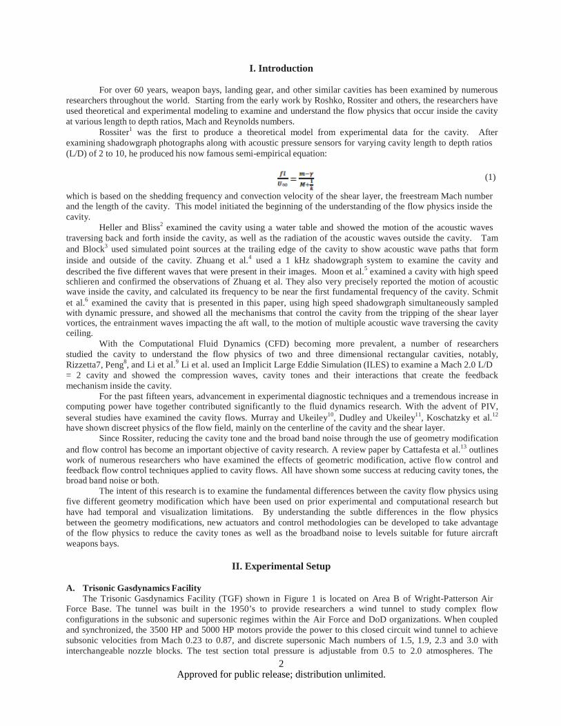
The Trisonic Gasdynamics Facility (TGF) shown in Figure 1 is located on Area B of Wright-Patterson Air Force Base. The tunnel was built in the 1950’s to provide researchers a wind tunnel to study complex flow configurations in the subsonic and supersonic regimes within the Air Force and DoD organizations. When coupled and synchronized, the 3500 HP and 5000 HP motors provide the power to this closed circuit wind tunnel to achieve subsonic velocities from Mach 0.23 to 0.87, and discrete supersonic Mach numbers of 1.5, 1.9, 2.3 and 3.0 with interchangeable nozzle blocks. The test section total pressure is adjustable from 0.5 to 2.0 atmospheres. The
3 Approved for public release; distribution unlimited.
maximum subsonic Reynolds number for the tunnel is 2.5 million per foot and the maximum subsonic dynamic pressure is 350 psf. The maximum supersonic Reynolds number is 5 million per foot and the maximum supersonic dynamic pressure is 1000 psf. The stagnation temperature is held constant at 75oF.
Figure 1. Trisonic Gasdynamics Facility
The test section is two feet high, two feet wide and four foot long with two optically flat 26 inch diameter viewing windows on either side of the test section. The primary model support is a crescent mounted sting, which can be used to reach various attitudes, or model orientations, including pitch from -1º to +18.5º, and roll from -90º to +180º. Refer to the TGF User’s Manual14 for more information and capabilities.
B. Optical Turbulence Reduction Cavity Model The original Turbulence Reduction Cavity model was tested several times from the mid 1970’s to the late
1980’s, and provided acoustic measurements and oil flow visualization inside the cavity as well as Schlieren photographs of the flow field outside of the cavity. At the time, these diagnostic techniques were still state of the art, though they had been around for a few decades15. With the subsequent development of state of the art non-intrusive flow field measuring techniques, i.e. Particle Image Velocimetry (PIV), Laser Doppler Anemometry (LDA) and Planar Induced Florescence (PLIF), the original Turbulence Reduction Cavity would not provide the necessary optical access for said techniques.
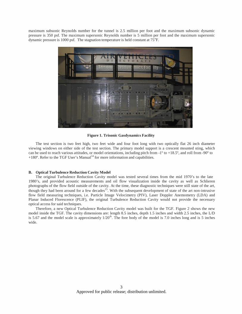
Therefore, a new Optical Turbulence Reduction Cavity model was built for the TGF. Figure 2 shows the new model inside the TGF. The cavity dimensions are: length 8.5 inches, depth 1.5 inches and width 2.5 inches, the L/D is 5.67 and the model scale is approximately 1/20th. The fore body of the model is 7.0 inches long and is 5 inches wide.
4 Approved for public release; distribution unlimited.
Figure 2. The Optical Turbulence Reduction Cavity mounted inside the TGF
The forward and aft wall blocks of the cavity are designed to be replaceable so that both passive and active flow
control devices are easy to insert without compromising overall geometry of the cavity during testing. This paper will cover results for the cavity at Mach 0.7 at a Reynolds numbers of 2 million per foot.
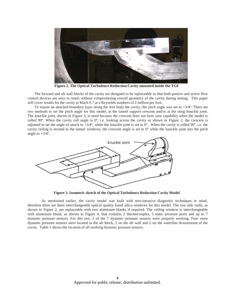
To ensure an attached boundary layer along the fore body the cavity, the pitch angle was set to +3/4º. There are two methods to set the pitch angle for this model, at the tunnel support crescent and/or at the sting knuckle joint. The knuckle joint, shown in Figure 3, is need because the crescent does not have yaw capability when the model is rolled 90º. When the cavity roll angle is 0º, i.e. looking across the cavity as shown in Figure 2, the crescent is adjusted to set the angle of attack to +3/4º, while the knuckle joint is set to 0º. When the cavity is rolled 90º, i.e. the cavity ceiling is normal to the tunnel windows, the crescent angle is set to 0º while the knuckle joint sets the pitch angle to +3/4º.
Knuckle Joint
Figure 3. Isometric sketch of the Optical Turbulence Reduction Cavity Model
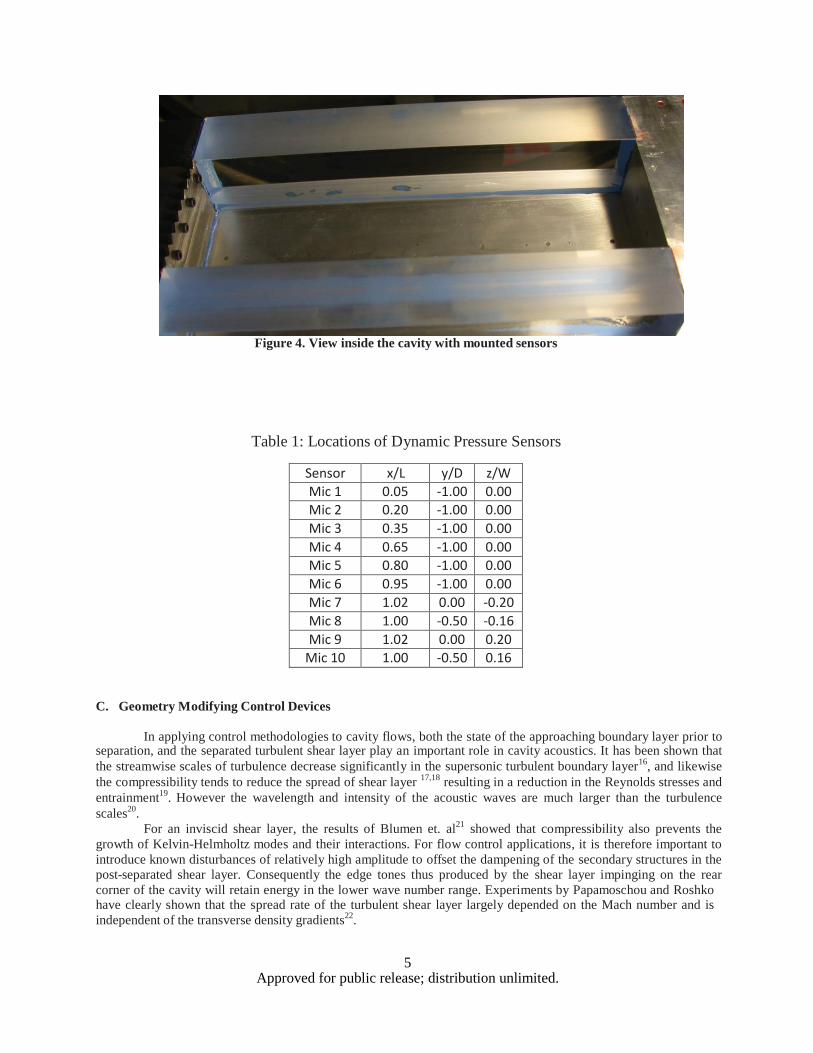
As mentioned earlier, the cavity model was built with non-intrusive diagnostic techniques in mind, therefore there are three interchangeable optical quality fused silica windows for this model. The two side walls, as shown in Figure 2, are replaceable with two aluminum blanks if required. The ceiling window is interchangeable with aluminum blank, as shown in Figure 4, that contains 2 thermocouples, 5 static pressure ports and up to 7 dynamic pressure sensors. For this test, 5 of the 7 dynamic pressure sensors were properly working. Four more dynamic pressure sensors were located in the aft block, 2 on the aft wall and 2 on the waterline downstream of the cavity. Table 1 shows the location of all working dynamic pressure sensors.
5 Approved for public release; distribution unlimited.
Figure 4. View inside the cavity with mounted sensors
Table 1: Locations of Dynamic Pressure Sensors
Sensor x/L y/D z/W Mic 1 0.05 -1.00 0.00 Mic 2 0.20 -1.00 0.00 Mic 3 0.35 -1.00 0.00 Mic 4 0.65 -1.00 0.00 Mic 5 0.80 -1.00 0.00 Mic 6 0.95 -1.00 0.00 Mic 7 1.02 0.00 -0.20 Mic 8 1.00 -0.50 -0.16 Mic 9 1.02 0.00 0.20
Mic 10 1.00 -0.50 0.16
C. Geometry Modifying Control Devices
In applying control methodologies to cavity flows, both the state of the approaching boundary layer prior to separation, and the separated turbulent shear layer play an important role in cavity acoustics. It has been shown that the streamwise scales of turbulence decrease significantly in the supersonic turbulent boundary layer16, and likewise the compressibility tends to reduce the spread of shear layer 17,18 resulting in a reduction in the Reynolds stresses and entrainment19. However the wavelength and intensity of the acoustic waves are much larger than the turbulence scales20.
For an inviscid shear layer, the results of Blumen et. al21 showed that compressibility also prevents the growth of Kelvin-Helmholtz modes and their interactions. For flow control applications, it is therefore important to introduce known disturbances of relatively high amplitude to offset the dampening of the secondary structures in the post-separated shear layer. Consequently the edge tones thus produced by the shear layer impinging on the rear corner of the cavity will retain energy in the lower wave number range. Experiments by Papamoschou and Roshko have clearly shown that the spread rate of the turbulent shear layer largely depended on the Mach number and is independent of the transverse density gradients22.
6 Approved for public release; distribution unlimited.
Recently Schulin and Trofimov reported that the vorticity generated by supercritical elements such as dots and triangular prisms placed in a supersonic turbulent boundary layer survived up to 104 times the height of the generators, and the disturbances amplified in the presence of adverse pressure gradient23. This shows the effectiveness of passive flow control techniques.
The passive flow control devices are broadly categorized as those applied to the leading edge and the trailing edge of a cavity. Leading edge devices include spoilers, wedges, cylinders, etc. and are primarily intended for the thickening of the separated shear layer24,25. The trailing edge treatment on the other hand is designed to deflect the shear layer and or acoustic wave by shaping of the rear wall26.
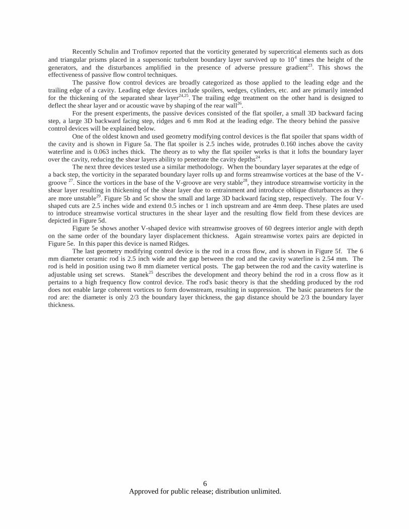
For the present experiments, the passive devices consisted of the flat spoiler, a small 3D backward facing step, a large 3D backward facing step, ridges and 6 mm Rod at the leading edge. The theory behind the passive control devices will be explained below.
One of the oldest known and used geometry modifying control devices is the flat spoiler that spans width of the cavity and is shown in Figure 5a. The flat spoiler is 2.5 inches wide, protrudes 0.160 inches above the cavity waterline and is 0.063 inches thick. The theory as to why the flat spoiler works is that it lofts the boundary layer over the cavity, reducing the shear layers ability to penetrate the cavity depths24.
The next three devices tested use a similar methodology. When the boundary layer separates at the edge of a back step, the vorticity in the separated boundary layer rolls up and forms streamwise vortices at the base of the V- groove 27. Since the vortices in the base of the V-groove are very stable28, they introduce streamwise vorticity in the shear layer resulting in thickening of the shear layer due to entrainment and introduce oblique disturbances as they are more unstable29. Figure 5b and 5c show the small and large 3D backward facing step, respectively. The four V- shaped cuts are 2.5 inches wide and extend 0.5 inches or 1 inch upstream and are 4mm deep. These plates are used to introduce streamwise vortical structures in the shear layer and the resulting flow field from these devices are depicted in Figure 5d.
Figure 5e shows another V-shaped device with streamwise grooves of 60 degrees interior angle with depth on the same order of the boundary layer displacement thickness. Again streamwise vortex pairs are depicted in Figure 5e. In this paper this device is named Ridges.
The last geometry modifying control device is the rod in a cross flow, and is shown in Figure 5f. The 6 mm diameter ceramic rod is 2.5 inch wide and the gap between the rod and the cavity waterline is 2.54 mm. The rod is held in position using two 8 mm diameter vertical posts. The gap between the rod and the cavity waterline is adjustable using set screws. Stanek25 describes the development and theory behind the rod in a cross flow as it pertains to a high frequency flow control device. The rod's basic theory is that the shedding produced by the rod does not enable large coherent vortices to form downstream, resulting in suppression. The basic parameters for the rod are: the diameter is only 2/3 the boundary layer thickness, the gap distance should be 2/3 the boundary layer thickness.
7 Approved for public release; distribution unlimited.
a. b.
c. d.
e. f Figure 5: The geometry modify flow control devices, a. Flat Spoiler, b. Small 3D backward facing steps, c. Large 3D backward facing step, d. Flow field of Figures 5b and 5c, e. Ridges, f. 6 mm Rod.
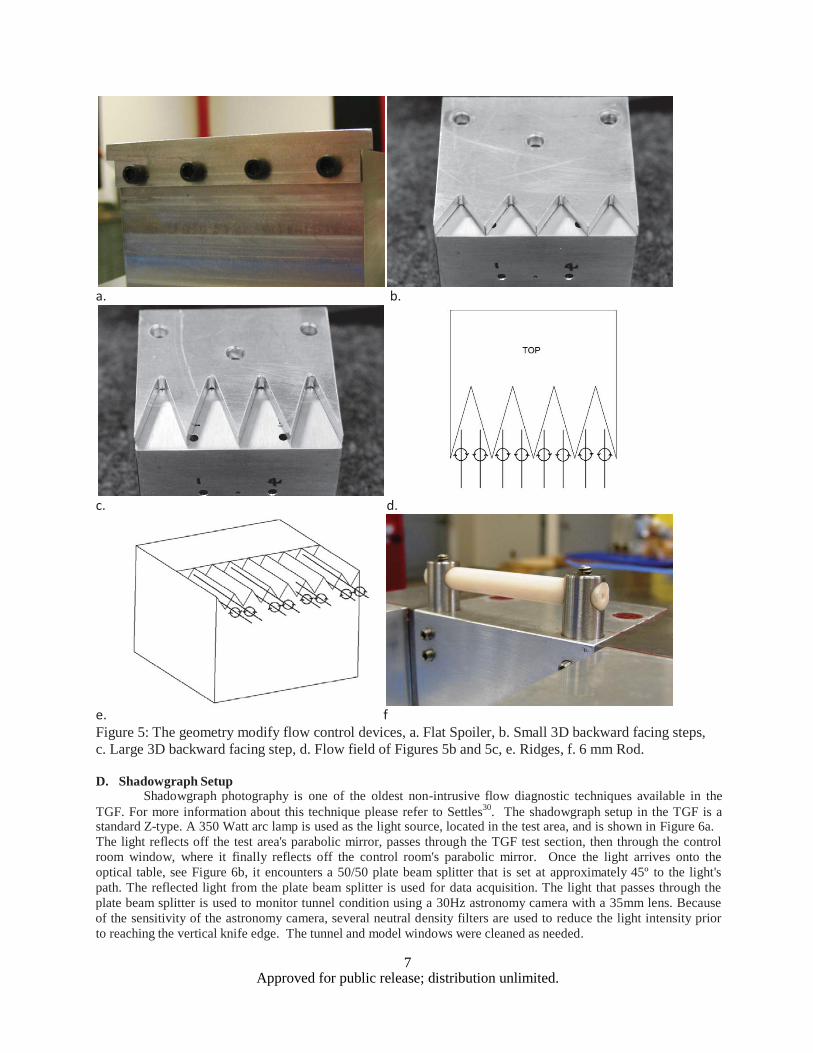
D. Shadowgraph Setup
Shadowgraph photography is one of the oldest non-intrusive flow diagnostic techniques available in the TGF. For more information about this technique please refer to Settles30. The shadowgraph setup in the TGF is a standard Z-type. A 350 Watt arc lamp is used as the light source, located in the test area, and is shown in Figure 6a. The light reflects off the test area's parabolic mirror, passes through the TGF test section, then through the control room window, where it finally reflects off the control room's parabolic mirror. Once the light arrives onto the optical table, see Figure 6b, it encounters a 50/50 plate beam splitter that is set at approximately 45º to the light's path. The reflected light from the plate beam splitter is used for data acquisition. The light that passes through the plate beam splitter is used to monitor tunnel condition using a 30Hz astronomy camera with a 35mm lens. Because of the sensitivity of the astronomy camera, several neutral density filters are used to reduce the light intensity prior to reaching the vertical knife edge. The tunnel and model windows were cleaned as needed.
8 Approved for public release; distribution unlimited.
a. b. Figure 6. Shadowgraph Optical Components. a. Light source with collimating optics. b. Receiving optics and
cameras
A Photron FASTCAM SA1 with an AF Zoom-NIKKOR 80-200 mm f/2.8D ED lens was used to capture the shadowgraph images. Because of the amount of light lost by a knife edge, the FASTCAM was setup for shadowgraph imaging. The camera's frame rate was set to 75000 Hz which provides a maximum resolution of 512 pixels horizontally by 128 pixels vertically. The electronic shutter speed was 1/2,700,000 sec., or 0.37 μsec. The pixel depth for this camera is 28 with three channels of color, RGB.
E. Data Acquisition and Analysis
The thermocouple data was sampled at 1 kHz, averaged, and recorded at 5 Hz using a National Instruments Data Acquisition card. The static pressure data was acquired with a Pressure Systems Model 8400 Scanner, at 100 Hz, averaged, and also recorded at 5 Hz. Both the temperature and static pressure sensors were check-calibrated in the model and have an uncertainty of 0.1% FS and 0.1% FS respectively. The dynamic pressure sensors were check-calibrated in the model and have an error uncertainty of 1.0% FS.
The dynamic pressure sensor data were acquired using the RBAX high-speed data (Whisper) system. This system performed simultaneous sample-and-hold acquisition at a rate of 75 kHz for data records 2 seconds in length. Digital images were simultaneously acquired during several dynamic pressure acquisition cycles. To accomplish image acquisition, a 5 V TTL trigger signal was sent from the high speed data acquisition system to the FASTCAM digital camera. The entire 2 seconds of high speed video was kept for only a handful of test points, since the ".avi" movie file size was 27.4 GB. For all other test points the first 5000 images were kept, which results in an ".avi" movie file size of just under 1GB. For the dynamic pressure data, each channel was 150,000 samples were collected.
A Discrete Fourier Transform (DFT) was used to convert the blocks of dynamic pressure and shadowgraph video data into the frequency domain. Prior to the DFT of the shadowgraph video, each pixel was converted from RGB to grayscale using Eq. (2).
(2) where I is the intensity of each pixel and R, G, and B is the individual intensity values for each of the color channels, Red, Green and Blue. The mean grayscale intensity was removed and one block of 4096 images was analyzed giving a δƒ of 18.31 Hz. Further analysis on the video images was not preformed.
Each dynamic pressure sensor was split into 37 blocks of 4096 samples resulting in a δƒ of 18.31 Hz. After determining the amplitude of the transformed pressure signal, the mean pressure amplitude is converted into sound pressure level using Eq. (3).
(3) where Pref is 2.9e-9 psi and n is the number of blocks.
9 Approved for public release; distribution unlimited.
Since sample frequency and consequently the DFT doesn't have an ideal response characteristic with a bandwidth of 1 Hz the sound pressure level needs to be converted to spectrum level using Eq. (4).
(4) where SR is the sample rate. To calculate the overall pressure level, the spectrum level is converted back to pressure using Eq. (5).
(5) Then the overall spectrum level, Eq. (6), is determined by integrating the pressure over the frequency spectrum and converting it back to a spectrum level.
(6) III. Results
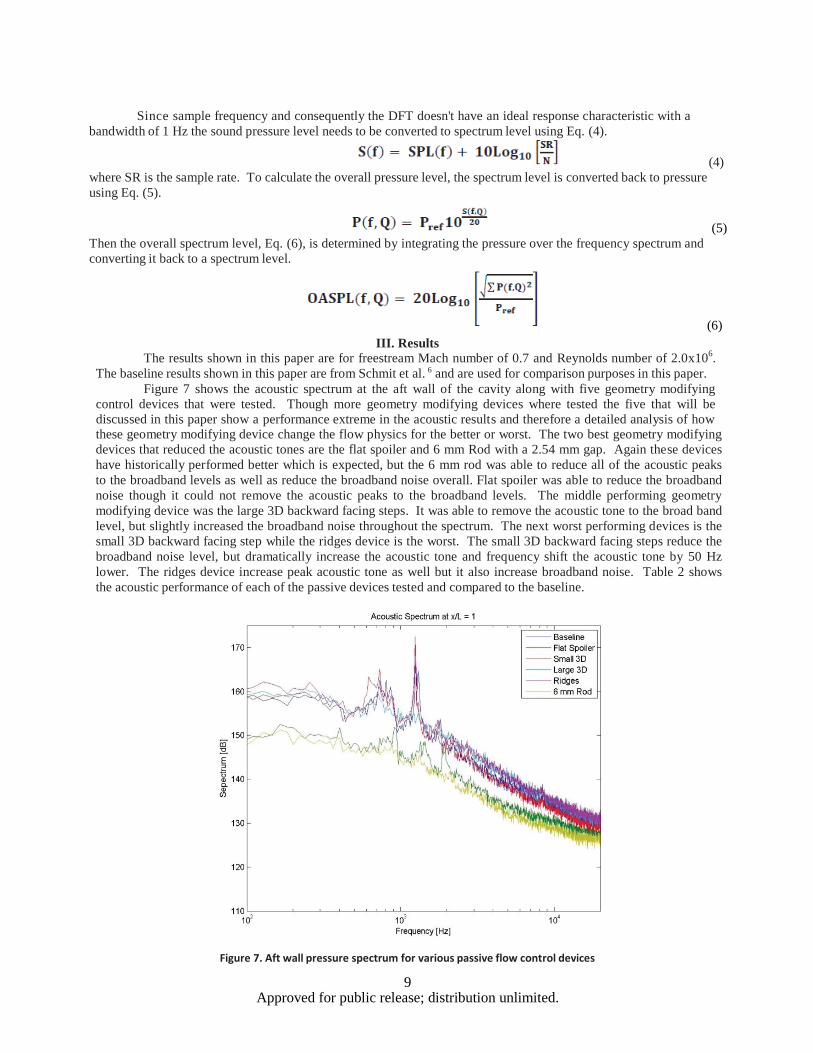
The results shown in this paper are for freestream Mach number of 0.7 and Reynolds number of 2.0x10⁶. The baseline results shown in this paper are from Schmit et al. 6 and are used for comparison purposes in this paper.
Figure 7 shows the acoustic spectrum at the aft wall of the cavity along with five geometry modifying control devices that were tested. Though more geometry modifying devices where tested the five that will be discussed in this paper show a performance extreme in the acoustic results and therefore a detailed analysis of how these geometry modifying device change the flow physics for the better or worst. The two best geometry modifying devices that reduced the acoustic tones are the flat spoiler and 6 mm Rod with a 2.54 mm gap. Again these devices have historically performed better which is expected, but the 6 mm rod was able to reduce all of the acoustic peaks to the broadband levels as well as reduce the broadband noise overall. Flat spoiler was able to reduce the broadband noise though it could not remove the acoustic peaks to the broadband levels. The middle performing geometry modifying device was the large 3D backward facing steps. It was able to remove the acoustic tone to the broad band level, but slightly increased the broadband noise throughout the spectrum. The next worst performing devices is the small 3D backward facing step while the ridges device is the worst. The small 3D backward facing steps reduce the broadband noise level, but dramatically increase the acoustic tone and frequency shift the acoustic tone by 50 Hz lower. The ridges device increase peak acoustic tone as well but it also increase broadband noise. Table 2 shows the acoustic performance of each of the passive devices tested and compared to the baseline.
Figure 7. Aft wall pressure spectrum for various passive flow control devices
10 Approved for public release; distribution unlimited.
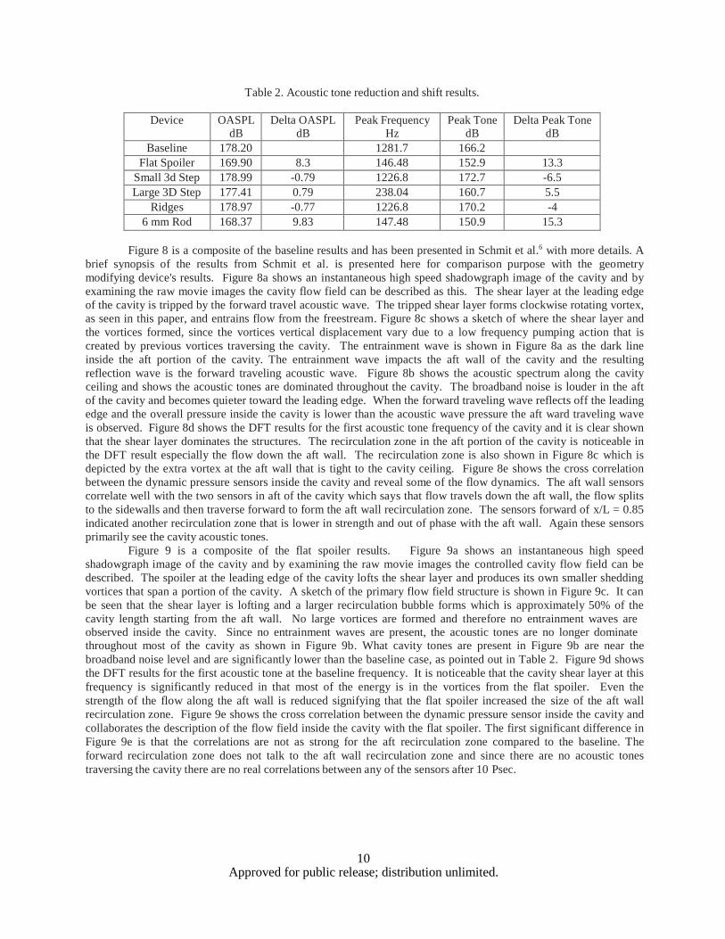
Table 2. Acoustic tone reduction and shift results.
Device OASPL dB
Delta OASPL dB
Peak Frequency Hz
Peak Tone dB
Delta Peak Tone dB
Baseline 178.20 1281.7 166.2 Flat Spoiler 169.90 8.3 146.48 152.9 13.3
Small 3d Step 178.99 -0.79 1226.8 172.7 -6.5 Large 3D Step 177.41 0.79 238.04 160.7 5.5
Ridges 178.97 -0.77 1226.8 170.2 -4 6 mm Rod 168.37 9.83 147.48 150.9 15.3
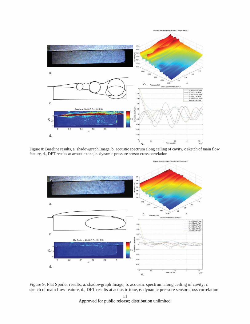
Figure 8 is a composite of the baseline results and has been presented in Schmit et al.6 with more details. A brief synopsis of the results from Schmit et al. is presented here for comparison purpose with the geometry modifying device's results. Figure 8a shows an instantaneous high speed shadowgraph image of the cavity and by examining the raw movie images the cavity flow field can be described as this. The shear layer at the leading edge of the cavity is tripped by the forward travel acoustic wave. The tripped shear layer forms clockwise rotating vortex, as seen in this paper, and entrains flow from the freestream. Figure 8c shows a sketch of where the shear layer and the vortices formed, since the vortices vertical displacement vary due to a low frequency pumping action that is created by previous vortices traversing the cavity. The entrainment wave is shown in Figure 8a as the dark line inside the aft portion of the cavity. The entrainment wave impacts the aft wall of the cavity and the resulting reflection wave is the forward traveling acoustic wave. Figure 8b shows the acoustic spectrum along the cavity ceiling and shows the acoustic tones are dominated throughout the cavity. The broadband noise is louder in the aft of the cavity and becomes quieter toward the leading edge. When the forward traveling wave reflects off the leading edge and the overall pressure inside the cavity is lower than the acoustic wave pressure the aft ward traveling wave is observed. Figure 8d shows the DFT results for the first acoustic tone frequency of the cavity and it is clear shown that the shear layer dominates the structures. The recirculation zone in the aft portion of the cavity is noticeable in the DFT result especially the flow down the aft wall. The recirculation zone is also shown in Figure 8c which is depicted by the extra vortex at the aft wall that is tight to the cavity ceiling. Figure 8e shows the cross correlation between the dynamic pressure sensors inside the cavity and reveal some of the flow dynamics. The aft wall sensors correlate well with the two sensors in aft of the cavity which says that flow travels down the aft wall, the flow splits to the sidewalls and then traverse forward to form the aft wall recirculation zone. The sensors forward of x/L = 0.85 indicated another recirculation zone that is lower in strength and out of phase with the aft wall. Again these sensors primarily see the cavity acoustic tones.
Figure 9 is a composite of the flat spoiler results. Figure 9a shows an instantaneous high speed shadowgraph image of the cavity and by examining the raw movie images the controlled cavity flow field can be described. The spoiler at the leading edge of the cavity lofts the shear layer and produces its own smaller shedding vortices that span a portion of the cavity. A sketch of the primary flow field structure is shown in Figure 9c. It can be seen that the shear layer is lofting and a larger recirculation bubble forms which is approximately 50% of the cavity length starting from the aft wall. No large vortices are formed and therefore no entrainment waves are observed inside the cavity. Since no entrainment waves are present, the acoustic tones are no longer dominate throughout most of the cavity as shown in Figure 9b. What cavity tones are present in Figure 9b are near the broadband noise level and are significantly lower than the baseline case, as pointed out in Table 2. Figure 9d shows the DFT results for the first acoustic tone at the baseline frequency. It is noticeable that the cavity shear layer at this frequency is significantly reduced in that most of the energy is in the vortices from the flat spoiler. Even the strength of the flow along the aft wall is reduced signifying that the flat spoiler increased the size of the aft wall recirculation zone. Figure 9e shows the cross correlation between the dynamic pressure sensor inside the cavity and collaborates the description of the flow field inside the cavity with the flat spoiler. The first significant difference in Figure 9e is that the correlations are not as strong for the aft recirculation zone compared to the baseline. The forward recirculation zone does not talk to the aft wall recirculation zone and since there are no acoustic tones traversing the cavity there are no real correlations between any of the sensors after 10 Psec.
11 Approved for public release; distribution unlimited.
Figure 8: Baseline results, a. shadowgraph Image, b. acoustic spectrum along ceiling of cavity, c sketch of main flow feature, d., DFT results at acoustic tone, e. dynamic pressure sensor cross correlation
Figure 9: Flat Spoiler results, a. shadowgraph Image, b. acoustic spectrum along ceiling of cavity, c sketch of main flow feature, d., DFT results at acoustic tone, e. dynamic pressure sensor cross correlation
12 Approved for public release; distribution unlimited.
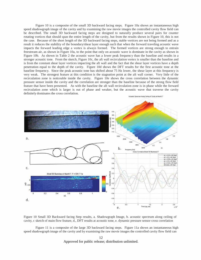
Figure 10 is a composite of the small 3D backward facing steps. Figure 10a shows an instantaneous high speed shadowgraph image of the cavity and by examining the raw movie images the controlled cavity flow field can be described. The small 3D backward facing steps are designed to naturally produce several pairs for counter rotating vortices that should span the entire length of the cavity, but from the results shown in Figure 10, this is not the case. Because of the short length of the 3D backward facing steps, stable vortices are not being formed and as a result it reduces the stability of the boundary/shear layer enough such that when the forward traveling acoustic wave impacts the forward leading edge a vortex is always formed. The formed vortices are strong enough to entrain freestream air, as shown in Figure 10a, to the point that only on acoustic wave is dominate in the cavity as shown in Figure 10b. As shown in Table 2 the acoustic wave has a lower peak frequency than the baseline and results in a stronger acoustic tone. From the sketch, Figure 10c, the aft wall recirculation vortex is smaller than the baseline and is from the constant shear layer vortices impacting the aft wall and the fact that the shear layer vortices have a depth penetration equal to the depth of the cavity. Figure 10d shows the DFT results for the first acoustic tone at the baseline frequency. Since the peak acoustic tone has shifted about 75 Hz lower, the shear layer at this frequency is very weak. The strongest feature at this condition is the stagnation point at the aft wall corner. Very little of the recirculation zone is noticeable inside the cavity. Figure 10e shows the cross correlation between the dynamic pressure sensor inside the cavity and the correlation are stronger than the baseline because of the strong flow field feature that have been presented. As with the baseline the aft wall recirculation zone is in phase while the forward recirculation zone which is larger is out of phase and weaker, but the acoustic wave that traverse the cavity definitely dominates the cross correlation.
Figure 10 Small 3D Backward facing Step results, a. Shadowgraph Image, b. acoustic spectrum along ceiling of cavity, c sketch of main flow feature, d., DFT results at acoustic tone, e. dynamic pressure sensor cross correlation
Figure 11 is a composite of the large 3D backward facing steps. Figure 11a shows an instantaneous high
speed shadowgraph image of the cavity and by examining the raw movie images the controlled cavity flow field can
13 Approved for public release; distribution unlimited.
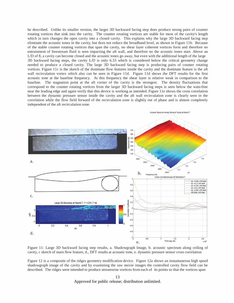
be described. Unlike its smaller version, the larger 3D backward facing step does produce strong pairs of counter rotating vortices that sink into the cavity. The counter rotating vortices are stable for most of the cavity's length which in turn changes the open cavity into a closed cavity. This explains why the large 3D backward facing step eliminate the acoustic tones in the cavity, but does not reduce the broadband level, as shown in Figure 11b. Because of the stable counter rotating vortices that span the cavity, no shear layer coherent vortices form and therefore no entrainment of freestream fluid is seen impacting the aft wall, and therefore no the acoustic tones start. Above an L/D of 8, a cavity can become closed and the acoustic tones go away, but even with the additional length of the large 3D backward facing steps, the cavity L/D is only 6.33 which is considered below the critical geometry change needed to produce a closed cavity. The large 3D backward facing step is producing pairs of counter rotating vortices. Figure 11c is the sketch of the dominate flow features inside the cavity and the dominate feature is the aft wall recirculation vortex which also can be seen in Figure 11d. Figure 11d shows the DFT results for the first acoustic tone at the baseline frequency. At this frequency the shear layer is relative weak in comparison to the baseline. The stagnation point at the aft corner of the cavity is the strongest. The density fluctuations that correspond to the counter rotating vortices from the larger 3D backward facing steps is seen below the wate rline near the leading edge and again verify that this device is working as intended. Figure 11e shows the cross correlation between the dynamic pressure sensor inside the cavity and the aft wall recirculation zone is clearly seen in the correlation while the flow field forward of the recirculation zone is slightly out of phase and is almost completely independent of the aft recirculation zone.
Figure 11: Large 3D backward facing step results, a. Shadowgraph Image, b. acoustic spectrum along ceiling of cavity, c sketch of main flow feature, d., DFT results at acoustic tone, e. dynamic pressure sensor cross correlation
Figure 12 is a composite of the ridges geometry modification device. Figure 12a shows an instantaneous high speed shadowgraph image of the cavity and by examining the raw movie images the controlled cavity flow field can be described. The ridges were intended to produce streamwise vortices from each of its points so that the vortices span
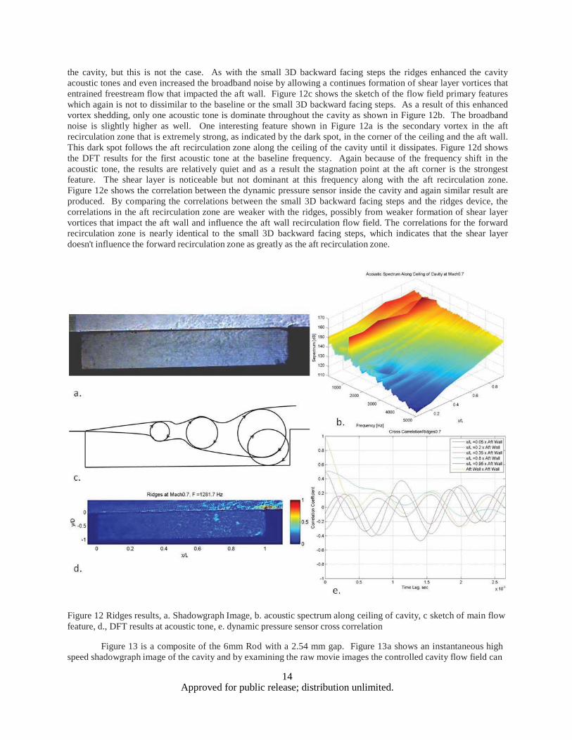
14 Approved for public release; distribution unlimited.
the cavity, but this is not the case. As with the small 3D backward facing steps the ridges enhanced the cavity acoustic tones and even increased the broadband noise by allowing a continues formation of shear layer vortices that entrained freestream flow that impacted the aft wall. Figure 12c shows the sketch of the flow field primary features which again is not to dissimilar to the baseline or the small 3D backward facing steps. As a result of this enhanced vortex shedding, only one acoustic tone is dominate throughout the cavity as shown in Figure 12b. The broadband noise is slightly higher as well. One interesting feature shown in Figure 12a is the secondary vortex in the aft recirculation zone that is extremely strong, as indicated by the dark spot, in the corner of the ceiling and the aft wall. This dark spot follows the aft recirculation zone along the ceiling of the cavity until it dissipates. Figure 12d shows the DFT results for the first acoustic tone at the baseline frequency. Again because of the frequency shift in the acoustic tone, the results are relatively quiet and as a result the stagnation point at the aft corner is the strongest feature. The shear layer is noticeable but not dominant at this frequency along with the aft recirculation zone. Figure 12e shows the correlation between the dynamic pressure sensor inside the cavity and again similar result are produced. By comparing the correlations between the small 3D backward facing steps and the ridges device, the correlations in the aft recirculation zone are weaker with the ridges, possibly from weaker formation of shear layer vortices that impact the aft wall and influence the aft wall recirculation flow field. The correlations for the forward recirculation zone is nearly identical to the small 3D backward facing steps, which indicates that the shear layer doesn't influence the forward recirculation zone as greatly as the aft recirculation zone.
Figure 12 Ridges results, a. Shadowgraph Image, b. acoustic spectrum along ceiling of cavity, c sketch of main flow feature, d., DFT results at acoustic tone, e. dynamic pressure sensor cross correlation
Figure 13 is a composite of the 6mm Rod with a 2.54 mm gap. Figure 13a shows an instantaneous high
speed shadowgraph image of the cavity and by examining the raw movie images the controlled cavity flow field can
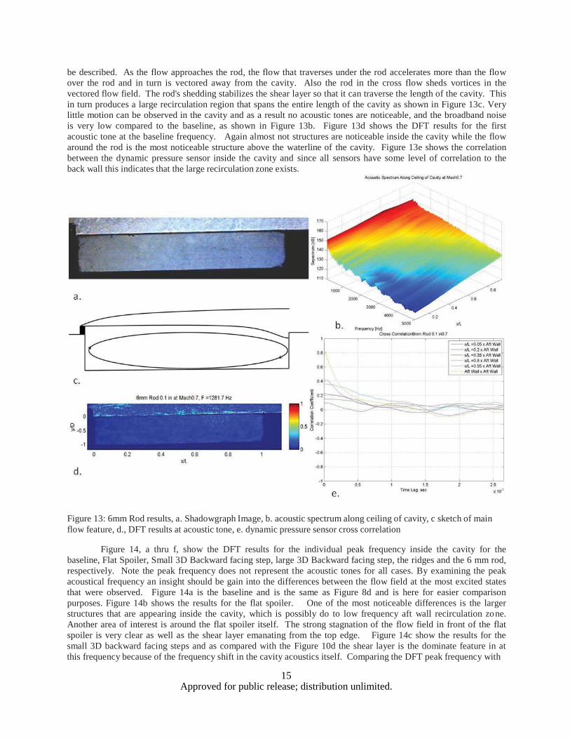
15 Approved for public release; distribution unlimited.
be described. As the flow approaches the rod, the flow that traverses under the rod accelerates more than the flow over the rod and in turn is vectored away from the cavity. Also the rod in the cross flow sheds vortices in the vectored flow field. The rod's shedding stabilizes the shear layer so that it can traverse the length of the cavity. This in turn produces a large recirculation region that spans the entire length of the cavity as shown in Figure 13c. Very little motion can be observed in the cavity and as a result no acoustic tones are noticeable, and the broadband noise is very low compared to the baseline, as shown in Figure 13b. Figure 13d shows the DFT results for the first acoustic tone at the baseline frequency. Again almost not structures are noticeable inside the cavity while the flow around the rod is the most noticeable structure above the waterline of the cavity. Figure 13e shows the correlation between the dynamic pressure sensor inside the cavity and since all sensors have some level of correlation to the back wall this indicates that the large recirculation zone exists.
Figure 13: 6mm Rod results, a. Shadowgraph Image, b. acoustic spectrum along ceiling of cavity, c sketch of main flow feature, d., DFT results at acoustic tone, e. dynamic pressure sensor cross correlation
Figure 14, a thru f, show the DFT results for the individual peak frequency inside the cavity for the
baseline, Flat Spoiler, Small 3D Backward facing step, large 3D Backward facing step, the ridges and the 6 mm rod, respectively. Note the peak frequency does not represent the acoustic tones for all cases. By examining the peak acoustical frequency an insight should be gain into the differences between the flow field at the most excited states that were observed. Figure 14a is the baseline and is the same as Figure 8d and is here for easier comparison purposes. Figure 14b shows the results for the flat spoiler. One of the most noticeable differences is the larger structures that are appearing inside the cavity, which is possibly do to low frequency aft wall recirculation zo ne. Another area of interest is around the flat spoiler itself. The strong stagnation of the flow field in front of the flat spoiler is very clear as well as the shear layer emanating from the top edge. Figure 14c show the results for the small 3D backward facing steps and as compared with the Figure 10d the shear layer is the dominate feature in at this frequency because of the frequency shift in the cavity acoustics itself. Comparing the DFT peak frequency with
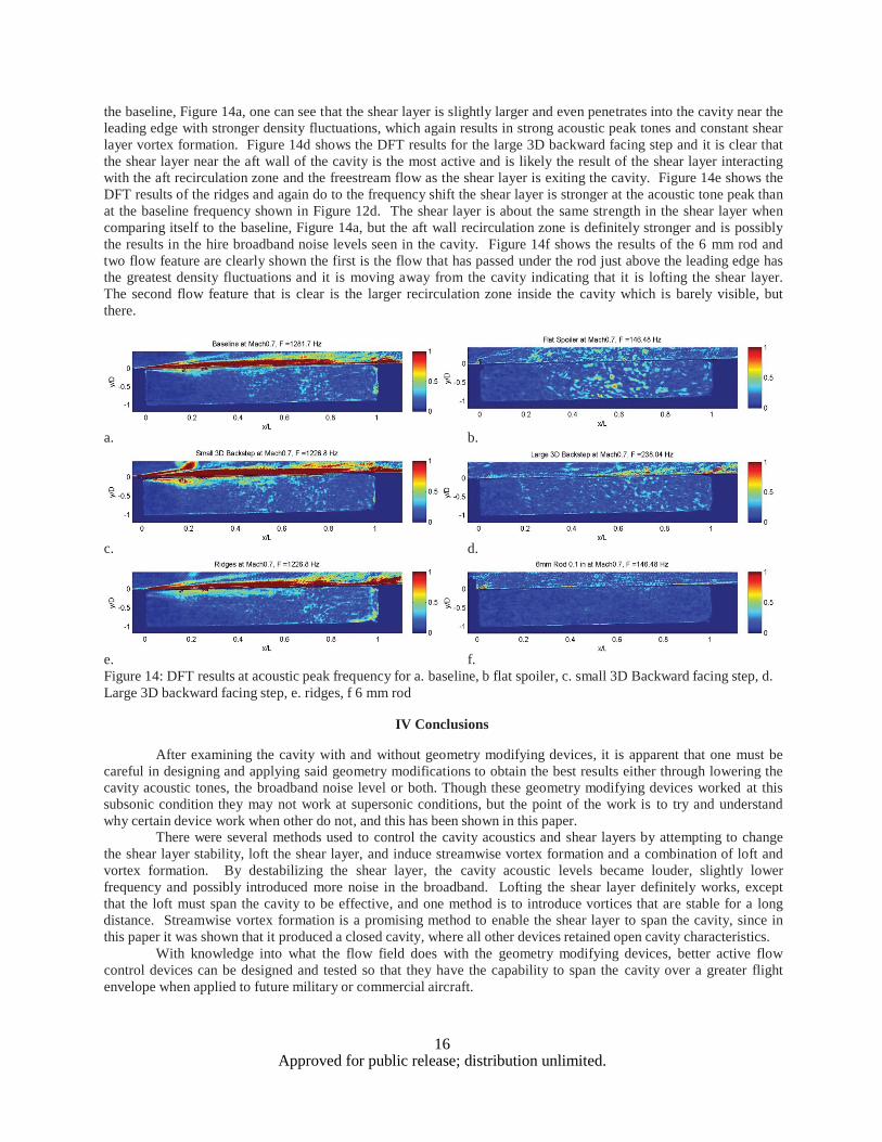
16 Approved for public release; distribution unlimited.
the baseline, Figure 14a, one can see that the shear layer is slightly larger and even penetrates into the cavity near the leading edge with stronger density fluctuations, which again results in strong acoustic peak tones and constant shear layer vortex formation. Figure 14d shows the DFT results for the large 3D backward facing step and it is clear that the shear layer near the aft wall of the cavity is the most active and is likely the result of the shear layer interacting with the aft recirculation zone and the freestream flow as the shear layer is exiting the cavity. Figure 14e shows the DFT results of the ridges and again do to the frequency shift the shear layer is stronger at the acoustic tone peak than at the baseline frequency shown in Figure 12d. The shear layer is about the same strength in the shear layer when comparing itself to the baseline, Figure 14a, but the aft wall recirculation zone is definitely stronger and is possibly the results in the hire broadband noise levels seen in the cavity. Figure 14f shows the results of the 6 mm rod and two flow feature are clearly shown the first is the flow that has passed under the rod just above the leading edge has the greatest density fluctuations and it is moving away from the cavity indicating that it is lofting the shear layer. The second flow feature that is clear is the larger recirculation zone inside the cavity which is barely visible, but there.
a. b.
c. d.
e. f. Figure 14: DFT results at acoustic peak frequency for a. baseline, b flat spoiler, c. small 3D Backward facing step, d. Large 3D backward facing step, e. ridges, f 6 mm rod
IV Conclusions
After examining the cavity with and without geometry modifying devices, it is apparent that one must be
careful in designing and applying said geometry modifications to obtain the best results either through lowering the cavity acoustic tones, the broadband noise level or both. Though these geometry modifying devices worked at this subsonic condition they may not work at supersonic conditions, but the point of the work is to try and understand why certain device work when other do not, and this has been shown in this paper.
There were several methods used to control the cavity acoustics and shear layers by attempting to change the shear layer stability, loft the shear layer, and induce streamwise vortex formation and a combination of loft and vortex formation. By destabilizing the shear layer, the cavity acoustic levels became louder, slightly lower frequency and possibly introduced more noise in the broadband. Lofting the shear layer definitely works, except that the loft must span the cavity to be effective, and one method is to introduce vortices that are stable for a long distance. Streamwise vortex formation is a promising method to enable the shear layer to span the cavity, since in this paper it was shown that it produced a closed cavity, where all other devices retained open cavity characteristics.
With knowledge into what the flow field does with the geometry modifying devices, better active flow control devices can be designed and tested so that they have the capability to span the cavity over a greater flight envelope when applied to future military or commercial aircraft.
17 Approved for public release; distribution unlimited.
References
1Rossiter, J. E., “Wind-Tunnel Experiments on the Flow over Rectangular Cavities at Subsonic and Transonic Speeds” London: Ministry of Aviation, Report and Memoranda No. 3438, 1966. 2Heller, H. H., and Bliss, D., "The Physical Mechanism of Flow-Induced Pressure Fluctuations in Cavities and Concepts of their Suppression," AIAA paper 75-491, 2nd Aeroacoustic Conference, Hampton VA 1975 3Tam, C. K., and Block, P. J, “On the Tones and Pressure Oscillations induced by Flow Over Rectangular Caviteis,” Journal of Fluid Mechanics, Vol 89 (part 2), 1978, pp. 373-399. 4Zhuang, N., Alvi, F. S., Alkislar, M. B., and Shih, C., “Supersonic Cavity Flows and Their Control,” AIAA Journal, Vol 44, No. 9, Sep. 2006, pp. 2118-2128. 5Moon, S. J., Gai, S. L., Kleine, H. H., and Neely, A. J., “Supersonic Flow Over Straight Shallow Caviies In Leading and Trailing Edge Modification,” 28th AIAA Applied Aerodynamic Conference, Chicago IL, 2010, pp. 1-11, AIAA 2010-4687 6Schmit, R.. F., Semmelmayer, F., Haverkamp, M.., and Grove, J., "Fourier Analysis of High Speed Shadowgraph Images around a Mach 1.5 Cavity Flow Field", 29th AIAA Applied Aerodynamic Conference, Honolulu, HI, 2011, pp. 1-24, AIAA 2011-3961 7Rizzetta, D. P., and Visbal, M. R., “Large-Eddy simulation of superonic cavity flow-fields including flow control,” AIAA Journal, Vol. 41, No. 8, Aug. 2003, pp. 1452-1462. 8Peng, S.-H., “Simulation of Turblent Flow Past a Rectangluar Open Cavity Using DES and Unsteady RANS,” 24th AIAA Applied Aerodaynmaics Conference, San Francisco, CA, 2006, pp. 1-20, AIAA 2006-2827 9Li, W., Nonomura, T., and Fujii, K., “Effects of shear-layer charateristic on the Feedback-loop Mechanism in supersonic open cavity flows,” 49th AIAA Aerospace Sciences Meeting including the New Horizons Forum and Aerospace Exposition, Orlando, FL, 2011, pp. 1- 12, AIAA 2011-1218 10Murray, N., and Ukeiley, L. “An application in Gappy POD”, Experiments in Fluids Vol 42, No. 1, Jan. 2007, pp. 79-91. 11Dudley, J. G., and Ukeiley, L. “Suppresion of Fluctuating Surface Pressure in a Supersonic Cavity Flow,” 5th Flow Control Conference, Chicago, IL, 2010, pp. 1-22, AIAA 2010-4974 12Koschatzky, V., Westerweel, J., and Boersma, B. J., “Comparison of two ascostic analogies applied experimental PIV data for cavity sound emission estimation,” 16th AIAA/CEAS Aeroacoustic Conference, 2010, pp. 1-11, AIAA 2010-3812. 13Cattafesta, L., N., Song, Q., Willimas, D., R., Rowley, C., W., and Alvi, F., S.,"Active Control of Flow-Induced Cavity Oscillations," Progress in Aerospace Sciences, Vol. 44, 2008, pp. 479-502 14Clark, G. F. “Trisonic Gasdynamic Facility User Manual,” Air Force Wright Aeronautical Laboratories Wright-Patterson AFB, AFWAL-TM-82-176-FIMM, 1982. 15Kaufman, L. G. and Clark, R. L. “Mach 0.6 to 3.0 Flows Over Rectangular Cavities,” Air Force Wright Aeronautical Laboratories, Wright-Patterson AFB, AFWAL-TR-82-3112, 1983. 16Dussauge, J. P, Smits A J., 1997, "Characteristic scales for energetic eddies in turbulent supersonic boundary layers," Experimental Thermal and Fluid Sciences, Vol. 14, pp. 85-91 17Birch, S. L and Eggers, J. M., 1973, "A critical review of experimental data for developed free turbulent shear layers," NASA SP321, pp. 943-949 18Pantano, C. and Sarkar, S., "A study of compressibility effects in the high-speed turbulent shear layer using direct simulation" Journal of Fluid Mechanics, Vol 14 2002, pp. 329-371 19Clemens, N T., Mungal M G., 1995, Large-scale structures and entrainment in supersonic mixing layer, J. Fluid Mech., 248, pp. 171-16 20Lilley G M., 2008, The generation of sound in turbulent motion, Aeronautical Journal, 112, pp. 381-394 21Blumen W., Dazing P G., Billings D F., 1975, Shear layer instability of inviscid compressible fluid, Part 2. J. Fluid Mech., 71, pp. 305-316 22Papamoschou D., Roshko A., 1988, The compressible turbulent shear layer: an experimental study, J. Fluid Mech., 197, pp. 453-477 23Schulein E, Trofimov V M., 2011, Steady longitudinal vortices in supersonic turbulent separated flows. J. Fluid Mech. 672, pp. 451-476. 24Schmit, R. F., McGaha, C., Tekell, J., Grove, J., and Stanek, M., “Performance Results for the Optical Turbulence Reduction Cavity,” 47th AIAA Aerospace Science Meeting Including the New Horizons Forum and Aerospace Exposistion, Orlando FL, 2009, pp. 1-13, AIAA 2009-702 25Stanek, M. J., Visbal, M. R., Rizzetta, D. P., Rubin, S. G., and Khosla, P. K., “On A Mechanism of Stabilizing Turbuelent Free Shear Layers in Cavity Flows,” Computers & Fluids, Vol 36, No 10 Dec 2007, pp 1621-1637. 26Zhang X., Rona A., Edwards J A., 1998, The effect of trailing edge geometry on cavity flow oscillations driven by a supersoni c shear layer. Aeronautical Journal 3, pp. 129-136 27Bar G L., 1972, Experimental investigation of the sudden expansion of a supersonic plane flow into a 90oVee channel. MS Thesis, Aerospace Engineering Department, Wichita State University, KS 28Ahmed, A., Zumwalt, G. W., 1993, Base Drag Reduction of a Non-Circular Missile, Journal of Spacecraft and Rockets, 30 (6) pp. 781-782 29Poggie, J., and Smits A. J., “Large Scale Structures in a Compressible Mixing Layer over a Cavity,” AIAA Journal, Vol. 41, No. 12, 2003, pp. 2410-2419 30Settles, G. S., Schlieren and Shadowgraph Techniques: Visualizing Phenomena in Transparent Media Springer, Berlin, 2006.