Embed Size (px)
Citation preview
1
ExaminingFile System Latency
in Production
Brendan Gregg, Lead Performance Engineer, Joyent
December, 2011
Abstract
This paper introduces file system latency as a metric for understanding application
performance. With the increased functionality and caching of file systems, the
traditional approach of studying disk-based metrics can be confusing and incomplete.
The different reasons for this will be explained in detail, including new behavior that has
been caused by I/O throttling in cloud computing environments. Solutions for
measuring file system latency are demonstrated, including the use of DTrace to create
custom analysis tools. We also show different ways this metric can be presented,
including the use of heat maps to visualize the full distribution of file system latency,
from Joyent’s Cloud Analytics.
2
Contents
1. When iostat Leads You Astray 4
1.1. Disk I/O 41.2. Other Processes 51.3. The I/O Stack 51.4. File Systems in the I/O Stack 61.5. I/O Inflation 71.6. I/O Deflation 71.7. Considering Disk I/O for Understanding Application I/O 8
2. Invisible Issues of I/O 92.1. File System Latency 9
2.1.1. DRAM Cache Hits 102.1.2. Lock Latency 112.1.3. Queueing 122.1.4. Cache Flush 13
2.2. Issues Missing from Disk I/O 15
3. Measuring File System Latency from Applications 163.1. File System Latency Distribution 163.2. Comparing to iostat(1M) 183.3. What It Isn’t 183.4. Presentation 193.5. Distribution Script 19
3.5.1. mysqld_pid_fslatency.d 203.5.2. Script Caveats 213.5.3. CPU Latency 21
3.6. Slow Query Logger 233.6.1. mysqld_pid_fslatency_slowlog.d 233.6.2. Interpreting Totals 253.6.3. Script Caveats 26
3.7. Considering File System Latency 26
4. Drilling Down Into the Kernel 28
4.1. Syscall Tracing 284.1.1. syscall-read-zfs.d 29
4.2. Stack Fishing 304.3. VFS Tracing 334.4. VFS Latency 344.5. File System Tracing 36
4.5.1. ZFS 374.6. Lower Level 38
4.6.1. zfsstacklatency.d 424.7. Comparing File System Latency 42
5. Presenting File System Latency 435.1. A Little History 43
5.1.1. kstats 455.1.2. truss, strace 45
3
5.1.3. LatencyTOP 455.1.4. SystemTap 465.1.5. Applications 465.1.6. MySQL 46
5.2. What’s Happening Now 475.3. What’s Next 485.4. vfsstat(1M) 48
5.4.1. kstats 495.4.2. Monitoring 495.4.3. man page 505.4.4. I/O Throttling 515.4.5. Averages 52
5.5. Cloud Analytics 525.5.1. Outliers 535.5.2. The 4th Dimension 545.5.3. Time-Based Patterns 545.5.4. Other Breakdowns 555.5.5. Context 565.5.6. And More 565.5.7. Reality Check 56
6. Conclusion 59
References 60
4
1. When iostat Leads You AstrayWhen examining system performance problems, we commonly point the finger of blame at the
system disks by observing disk I/O. This is a bottom-up approach to performance analysis: starting with the physical devices and moving up through the software stack. Such an approach
is standard for system administrators, who are responsible for these physical devices.
To understand the impact of I/O performance on applications, however, file systems can prove to be a better target for analysis than disks. Because modern file systems use more DRAM-
based cache and perform more asynchronous disk I/O, the performance perceived by an application can be very different from what’s happening on disk. I’ll demonstrate this by
examining the I/O performance of a MySQL database at both the disk and file system level.
We will first discuss the commonly-used approach, disk I/O analysis using iostat(1M), then turn to file system analysis using DTrace.
1.1. Disk I/O
When trying to understand how disk I/O affects application performance, analysis has historically
focused on the performance of storage-level devices: the disks themselves. This includes the use of tools such as iostat(1M), which prints various I/O statistics for disk devices. System administrators either run iostat(1M) directly at the command line, or use it via another interface.
Some monitoring software (e.g., munin) will use iostat(1M) to fetch the disk statistics which they then archive and plot.
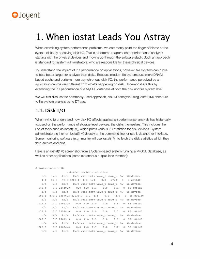
Here is an iostat(1M) screenshot from a Solaris-based system running a MySQL database, as well as other applications (some extraneous output lines trimmed):
# iostat -xnz 1 10
extended device statistics
r/s w/s kr/s kw/s wait actv wsvc_t asvc_t %w %b device
1.1 33.8 78.8 1208.1 0.0 1.0 0.0 27.8 0 4 c0t1d0
r/s w/s kr/s kw/s wait actv wsvc_t asvc_t %w %b device
175.4 0.0 22449.9 0.0 0.0 1.1 0.0 6.1 0 82 c0t1d0
r/s w/s kr/s kw/s wait actv wsvc_t asvc_t %w %b device
106.1 379.2 13576.5 22036.7 0.0 2.4 0.0 4.9 0 85 c0t1d0
r/s w/s kr/s kw/s wait actv wsvc_t asvc_t %w %b device
139.9 0.0 17912.6 0.0 0.0 1.0 0.0 6.8 0 82 c0t1d0
r/s w/s kr/s kw/s wait actv wsvc_t asvc_t %w %b device
176.1 0.0 22538.0 0.0 0.0 1.0 0.0 5.7 0 85 c0t1d0
r/s w/s kr/s kw/s wait actv wsvc_t asvc_t %w %b device
208.0 0.0 26619.9 0.0 0.0 1.9 0.0 9.2 0 99 c0t1d0
r/s w/s kr/s kw/s wait actv wsvc_t asvc_t %w %b device
208.0 0.0 26624.4 0.0 0.0 1.7 0.0 8.2 0 95 c0t1d0
r/s w/s kr/s kw/s wait actv wsvc_t asvc_t %w %b device
5
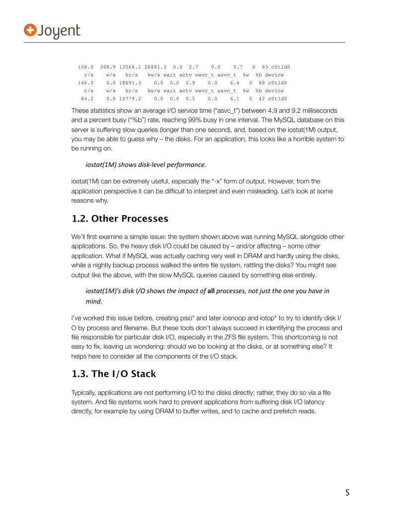
106.0 368.9 13566.1 26881.3 0.0 2.7 0.0 5.7 0 93 c0t1d0
r/s w/s kr/s kw/s wait actv wsvc_t asvc_t %w %b device
146.0 0.0 18691.3 0.0 0.0 0.9 0.0 6.4 0 88 c0t1d0
r/s w/s kr/s kw/s wait actv wsvc_t asvc_t %w %b device
84.2 0.0 10779.2 0.0 0.0 0.5 0.0 6.1 0 42 c0t1d0
These statistics show an average I/O service time (“asvc_t”) between 4.9 and 9.2 milliseconds and a percent busy (“%b”) rate, reaching 99% busy in one interval. The MySQL database on this
server is suffering slow queries (longer than one second), and, based on the iostat(1M) output, you may be able to guess why – the disks. For an application, this looks like a horrible system to be running on.
iostat(1M) shows disk-‐level performance.
iostat(1M) can be extremely useful, especially the “-x” form of output. However, from the
application perspective it can be difficult to interpret and even misleading. Let’s look at some reasons why.
1.2. Other Processes
We’ll first examine a simple issue: the system shown above was running MySQL alongside other applications. So, the heavy disk I/O could be caused by – and/or affecting – some other
application. What if MySQL was actually caching very well in DRAM and hardly using the disks, while a nightly backup process walked the entire file system, rattling the disks? You might see
output like the above, with the slow MySQL queries caused by something else entirely.
iostat(1M)’s disk I/O shows the impact of all processes, not just the one you have in
mind.
I’ve worked this issue before, creating psio* and later iosnoop and iotop* to try to identify disk I/
O by process and filename. But these tools don’t always succeed in identifying the process and file responsible for particular disk I/O, especially in the ZFS file system. This shortcoming is not easy to fix, leaving us wondering: should we be looking at the disks, or at something else? It
helps here to consider all the components of the I/O stack.
1.3. The I/O Stack
Typically, applications are not performing I/O to the disks directly; rather, they do so via a file system. And file systems work hard to prevent applications from suffering disk I/O latency directly, for example by using DRAM to buffer writes, and to cache and prefetch reads.
6
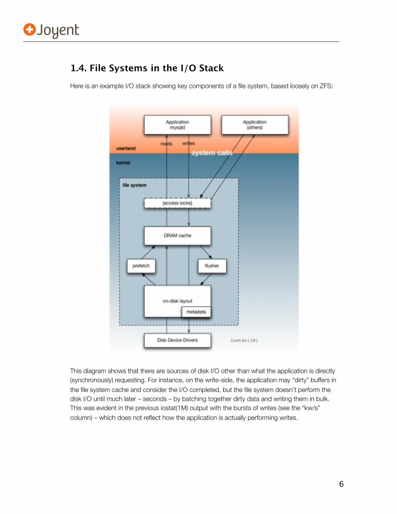
1.4. File Systems in the I/O Stack
Here is an example I/O stack showing key components of a file system, based loosely on ZFS:
This diagram shows that there are sources of disk I/O other than what the application is directly (synchronously) requesting. For instance, on the write-side, the application may “dirty” buffers in
the file system cache and consider the I/O completed, but the file system doesn’t perform the disk I/O until much later – seconds – by batching together dirty data and writing them in bulk. This was evident in the previous iostat(1M) output with the bursts of writes (see the “kw/s”
column) – which does not reflect how the application is actually performing writes.
7
1.5. I/O Inflation
Apart from other sources of disk I/O adding to the confusion, there is also what happens to the
direct I/O itself – particularly with the on-disk layout layer. This is a big topic I won’t go into much here, but I’ll enumerate a single example of I/O inflation to consider:
1. An application performs a 1 byte write to an existing file.
2. The file system identifies the location as part of a 128 Kbyte file system “record”, which is not cached (but the metadata to reference it is).
3. The file system requests the record be loaded from disk.
4. The disk device layer breaks the 128 Kbyte read into smaller reads suitable for the device.
5. The disks perform multiple smaller reads, totaling 128 Kbytes.
6. The file system now replaces the 1 byte in the record with the new byte.
7. Sometime later, the file system requests the 128 Kbyte “dirty” record be written back to
disk.
8. The disks write the 128 Kbyte record (broken up if needed).
9. The file system writes new metadata; e.g., references (for Copy-On-Write), or atime (access
time).
10. The disks perform more writes.
So, while the application performed a single 1 byte write, the disks performed multiple reads (128 Kbytes worth) and even more writes (over 128 Kbytes worth).
ApplicaCon I/O to the file system != Disk I/O
It can be even worse than this, for example if the metadata required to reference the location had to be read in the first place, and if the file system (volume manager) employed RAID with a
stripe size larger than the record size.
1.6. I/O Deflation
Having mentioned inflation, I should also mention that deflation is possible (in case it isn’t obvious). Causes can include caching in DRAM to satisfy reads, and cancellation of buffered writes (data rewritten before it has been flushed to disk).
I’ve recently been watching production ZFS file systems running with a cache hit rate of over 99.9%, meaning that only a trickle of reads are actually reaching disk.
8
1.7. Considering Disk I/O for Understanding Application I/O
To summarize so far: looking at how hard the disks are rattling, as we did above using iostat(1M), tells us very little about what the target application is actually experiencing. Application I/O can be inflated or deflated by the file system by the time it reaches disks, making difficult at best
a direct correlation between disk and application I/O. Disk I/O also includes requests from other file system components, such as prefetch, the background flusher, on-disk layout metadata, and
other users of the file system (other applications). Even if you find an issue at the disk level, it’s hard to tell how much that matters to the application in question.
iostat(1M) includes other file system I/O, which may not directly affect the performance of the target applicaCon.
Summarizing the previous issues:
iostat(1M) shows disk level performance, not file system performance.
Next I’ll show how file system performance can be analyzed.
9
2. Invisible Issues of I/OI previously explained why disk I/O is difficult to associate with an application, and why it can be
altered from what the application requested. Now I’ll focus more on the file system, and show why it can be important to study I/O that never even reaches disk.
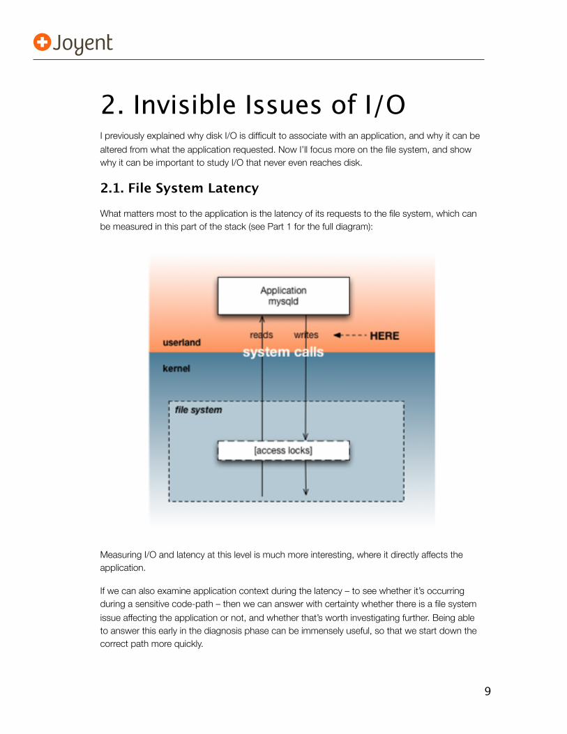
2.1. File System Latency
What matters most to the application is the latency of its requests to the file system, which can be measured in this part of the stack (see Part 1 for the full diagram):
Measuring I/O and latency at this level is much more interesting, where it directly affects the application.
If we can also examine application context during the latency – to see whether it’s occurring during a sensitive code-path – then we can answer with certainty whether there is a file system
issue affecting the application or not, and whether that’s worth investigating further. Being able to answer this early in the diagnosis phase can be immensely useful, so that we start down the correct path more quickly.
10
Apart from being more relevant to the application than disk I/O, file system I/O also includes of other phenomena that can be worth examining, including cache hits, lock latency, additional
queueing, and disk-cache flush latency.
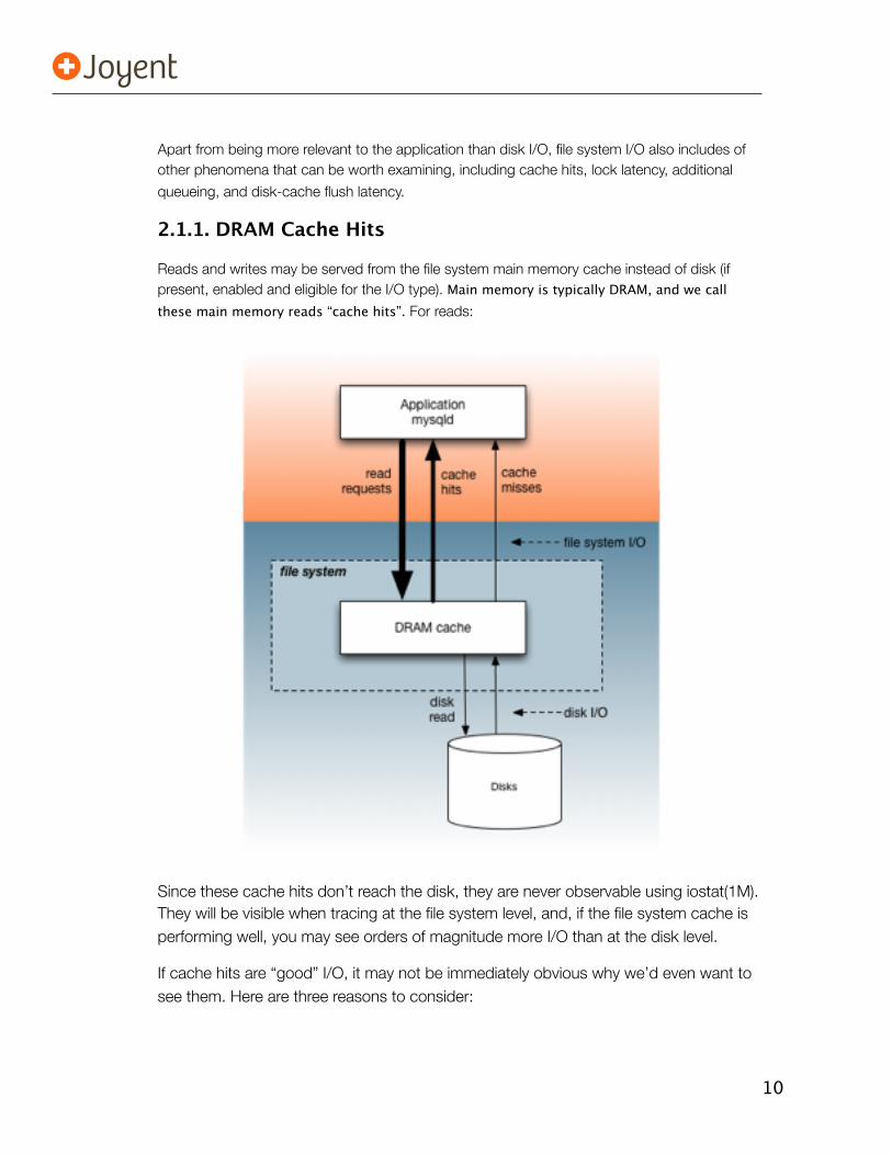
2.1.1. DRAM Cache Hits
Reads and writes may be served from the file system main memory cache instead of disk (if present, enabled and eligible for the I/O type). Main memory is typically DRAM, and we call these main memory reads “cache hits”. For reads:
Since these cache hits don’t reach the disk, they are never observable using iostat(1M). They will be visible when tracing at the file system level, and, if the file system cache is performing well, you may see orders of magnitude more I/O than at the disk level.
If cache hits are “good” I/O, it may not be immediately obvious why we’d even want to see them. Here are three reasons to consider:
11
• load analysis: by observing all requested I/O, you know exactly how the application is using the file system – the load applied – which may lead to tuning or capacity planning decisions.
• unnecessary work: identifying I/O that shouldn’t be sent to the file system to start with, whether it’s a cache hit or not.
• latency: cache hits may not be as fast as you think.
What if the I/O was slow due to file system lock contention, even though no disk I/O was involved?
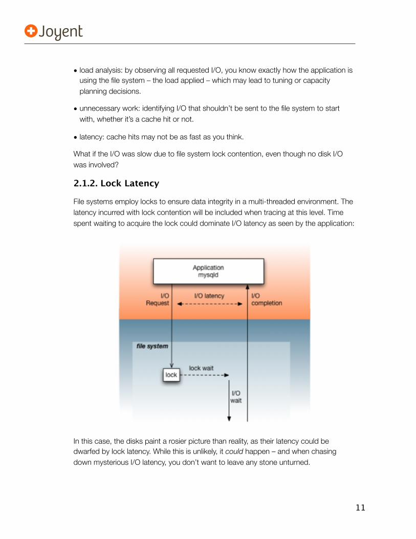
2.1.2. Lock Latency
File systems employ locks to ensure data integrity in a multi-threaded environment. The latency incurred with lock contention will be included when tracing at this level. Time spent waiting to acquire the lock could dominate I/O latency as seen by the application:
In this case, the disks paint a rosier picture than reality, as their latency could be dwarfed by lock latency. While this is unlikely, it could happen – and when chasing down mysterious I/O latency, you don’t want to leave any stone unturned.
12
High lock wait (contention) could happen for a number of reasons, including extreme I/O conditions or file system bugs (remember: the file system is software, and any software can have bugs). Lock and other sources of file system latency won’t be visible from iostat(1M).
If you only use iostat(1M), you may be flying blind regarding lock and other file
system issues.
There is one other latency source that iostat(1M) does show directly: waiting on one of the I/O queues. I’ll dig into queueing a little here, and explain why we need to return to file system latency.
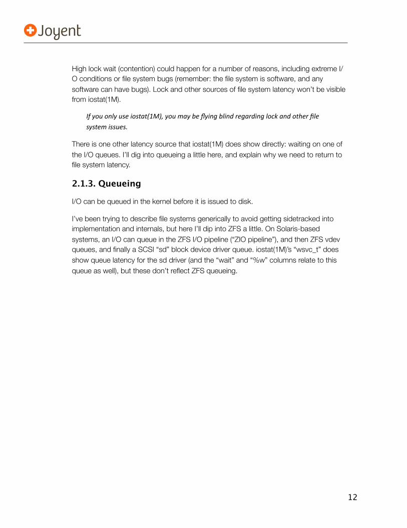
2.1.3. Queueing
I/O can be queued in the kernel before it is issued to disk.
I’ve been trying to describe file systems generically to avoid getting sidetracked into implementation and internals, but here I’ll dip into ZFS a little. On Solaris-based systems, an I/O can queue in the ZFS I/O pipeline (“ZIO pipeline”), and then ZFS vdev queues, and finally a SCSI “sd” block device driver queue. iostat(1M)’s “wsvc_t” does show queue latency for the sd driver (and the “wait” and “%w” columns relate to this queue as well), but these don’t reflect ZFS queueing.
13
So, iostat(1M) gets a brief reprieve – it doesn’t show just disk I/O latency, but also block device driver queue latency.
However, similarly to disk I/O latency, queue latency may not matter unless the application is waiting for that I/O to complete. To understand this from the application perspective, we are still best served by measuring latency at the file system level – which will include any queueing latency from any queue that the application I/O has synchronously waited for.
2.1.4. Cache Flush
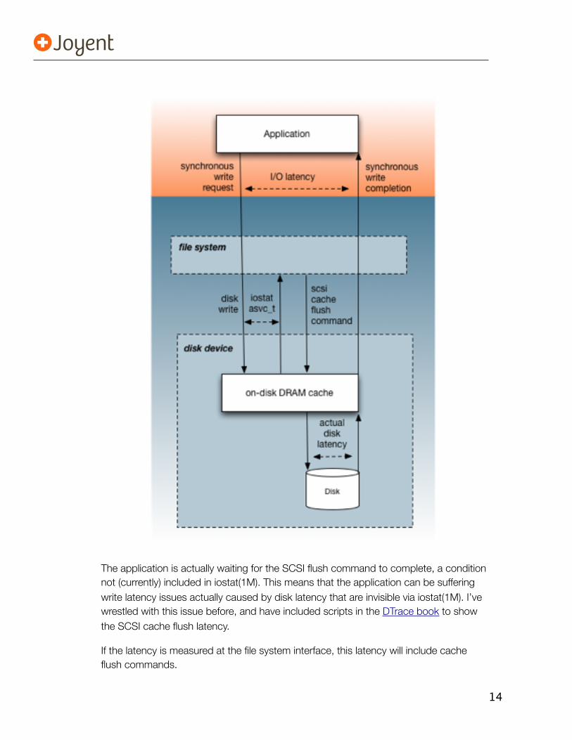
Some file systems ensure that synchronous write I/O – where the application has requested that the write not complete until it is on stable storage – really is on stable storage. (ZFS may actually be the only file system that currently does this by default.) It can work by sending SCSI cache flush commands to the disk devices, and not completing the application I/O until the cache flush command has completed. This ensures that the data really is on stable storage – and not just buffered.
14
The application is actually waiting for the SCSI flush command to complete, a condition not (currently) included in iostat(1M). This means that the application can be suffering write latency issues actually caused by disk latency that are invisible via iostat(1M). I’ve wrestled with this issue before, and have included scripts in the DTrace book to show the SCSI cache flush latency.
If the latency is measured at the file system interface, this latency will include cache flush commands.
15
2.2. Issues Missing from Disk I/O
Part 1 showed how application storage I/O was confusing to understand from the disk level. In this part I showed some scenarios where issues are just not visible. This isn’t really a failing of iostat(1M), which is a great tool for system administrators to understand the usage of their resources. But applications are far, far away from the disks, with a complex file system in between. For application analysis, iostat(1M) may provide clues that disks could be causing issues, but, in order to directly associate latency with the application, you really need to measure at the file system level, and consider other file system latency issues.
In the next section I’ll measure file system latency on a running application (MySQL).
16
3. Measuring File System Latency from ApplicationsHere we’ll show how you can measure file system I/O latency – the time spent waiting for the file system to complete I/O – from the applications themselves, and without modifying or even restarting them. This can save a lot of time when investigating disk I/O as a source of performance issues.
As an example application to study I chose a busy MySQL production server, and I’ll focus on using the DTrace pid provider to examine storage I/O. For an introduction to MySQL analysis with DTrace, see my blog posts on MySQL Query Latency. Here I’ll take that topic further, measuring the file system component of query latency.
3.1. File System Latency Distribution
I’ll start by showing some results of measuring this, and then the tool I used to do it.
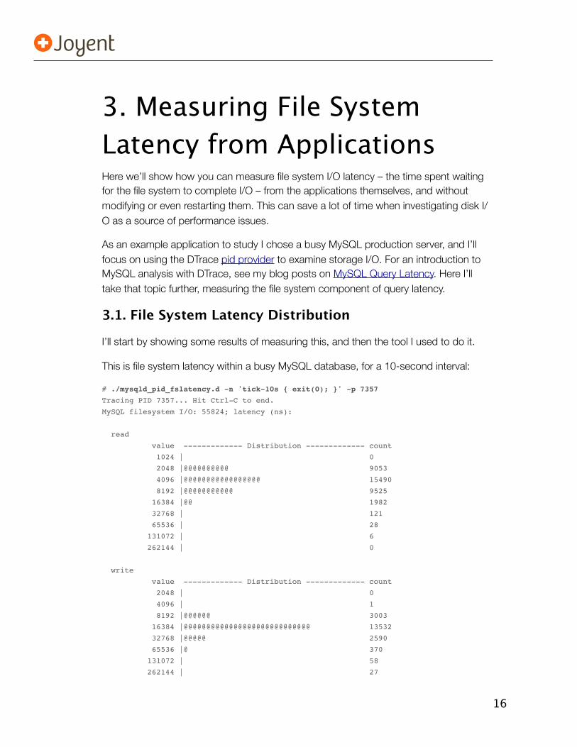
This is file system latency within a busy MySQL database, for a 10-second interval:
# ./mysqld_pid_fslatency.d -n 'tick-10s { exit(0); }' -p 7357
Tracing PID 7357... Hit Ctrl-C to end.
MySQL filesystem I/O: 55824; latency (ns):
read
value ------------- Distribution ------------- count
1024 | 0
2048 |@@@@@@@@@@ 9053
4096 |@@@@@@@@@@@@@@@@@ 15490
8192 |@@@@@@@@@@@ 9525
16384 |@@ 1982
32768 | 121
65536 | 28
131072 | 6
262144 | 0
write
value ------------- Distribution ------------- count
2048 | 0
4096 | 1
8192 |@@@@@@ 3003
16384 |@@@@@@@@@@@@@@@@@@@@@@@@@@@@ 13532
32768 |@@@@@ 2590
65536 |@ 370
131072 | 58
262144 | 27
17
524288 | 12
1048576 | 1
2097152 | 0
4194304 | 10
8388608 | 14
16777216 | 1
33554432 | 0
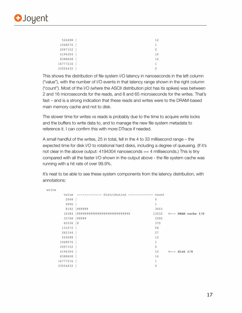
This shows the distribution of file system I/O latency in nanoseconds in the left column (“value”), with the number of I/O events in that latency range shown in the right column (“count”). Most of the I/O (where the ASCII distribution plot has its spikes) was between 2 and 16 microseconds for the reads, and 8 and 65 microseconds for the writes. That’s fast – and is a strong indication that these reads and writes were to the DRAM-based main memory cache and not to disk.
The slower time for writes vs reads is probably due to the time to acquire write locks and the buffers to write data to, and to manage the new file system metadata to reference it. I can confirm this with more DTrace if needed.
A small handful of the writes, 25 in total, fell in the 4 to 33 millisecond range – the expected time for disk I/O to rotational hard disks, including a degree of queueing. (If it’s not clear in the above output: 4194304 nanoseconds == 4 milliseconds.) This is tiny compared with all the faster I/O shown in the output above - the file system cache was running with a hit rate of over 99.9%.
It’s neat to be able to see these system components from the latency distribution, with annotations:
write
value ------------- Distribution ------------- count
2048 | 0
4096 | 1
8192 |@@@@@@ 3003
16384 |@@@@@@@@@@@@@@@@@@@@@@@@@@@@ 13532 <--- DRAM cache I/O
32768 |@@@@@ 2590
65536 |@ 370
131072 | 58
262144 | 27
524288 | 12
1048576 | 1
2097152 | 0
4194304 | 10 <--- disk I/O
8388608 | 14
16777216 | 1
33554432 | 0
18
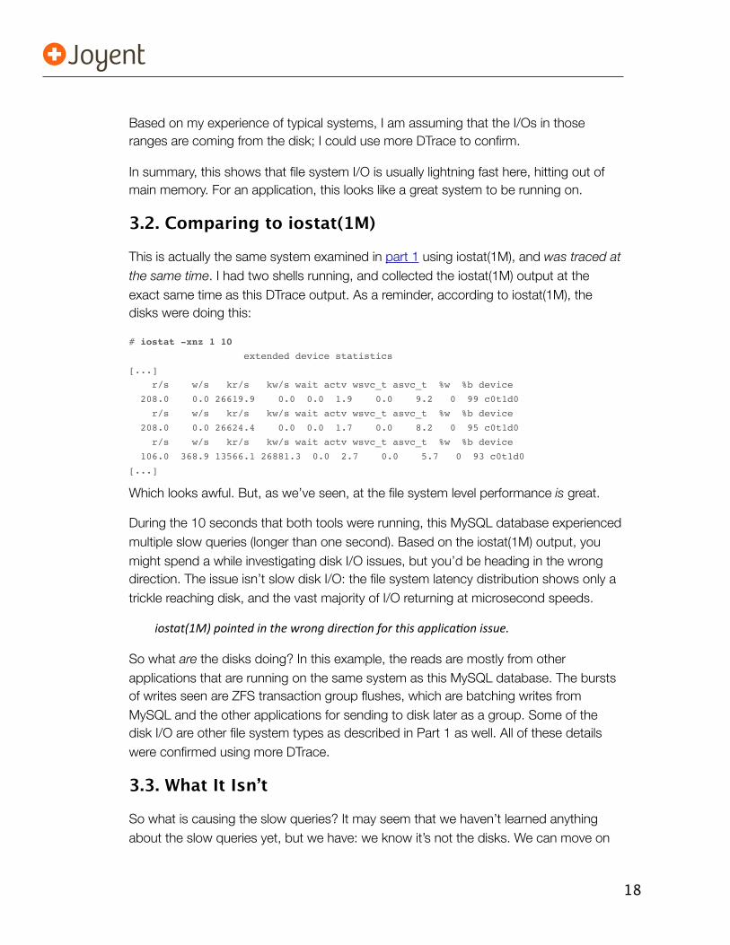
Based on my experience of typical systems, I am assuming that the I/Os in those ranges are coming from the disk; I could use more DTrace to confirm.
In summary, this shows that file system I/O is usually lightning fast here, hitting out of main memory. For an application, this looks like a great system to be running on.
3.2. Comparing to iostat(1M)
This is actually the same system examined in part 1 using iostat(1M), and was traced at the same time. I had two shells running, and collected the iostat(1M) output at the exact same time as this DTrace output. As a reminder, according to iostat(1M), the disks were doing this:
# iostat -xnz 1 10
extended device statistics
[...]
r/s w/s kr/s kw/s wait actv wsvc_t asvc_t %w %b device
208.0 0.0 26619.9 0.0 0.0 1.9 0.0 9.2 0 99 c0t1d0
r/s w/s kr/s kw/s wait actv wsvc_t asvc_t %w %b device
208.0 0.0 26624.4 0.0 0.0 1.7 0.0 8.2 0 95 c0t1d0
r/s w/s kr/s kw/s wait actv wsvc_t asvc_t %w %b device
106.0 368.9 13566.1 26881.3 0.0 2.7 0.0 5.7 0 93 c0t1d0
[...]
Which looks awful. But, as we’ve seen, at the file system level performance is great.
During the 10 seconds that both tools were running, this MySQL database experienced multiple slow queries (longer than one second). Based on the iostat(1M) output, you might spend a while investigating disk I/O issues, but you’d be heading in the wrong direction. The issue isn’t slow disk I/O: the file system latency distribution shows only a trickle reaching disk, and the vast majority of I/O returning at microsecond speeds.
iostat(1M) pointed in the wrong direcCon for this applicaCon issue.
So what are the disks doing? In this example, the reads are mostly from other applications that are running on the same system as this MySQL database. The bursts of writes seen are ZFS transaction group flushes, which are batching writes from MySQL and the other applications for sending to disk later as a group. Some of the disk I/O are other file system types as described in Part 1 as well. All of these details were confirmed using more DTrace.
3.3. What It Isn’t
So what is causing the slow queries? It may seem that we haven’t learned anything about the slow queries yet, but we have: we know it’s not the disks. We can move on
19
to searching other areas – the database itself, as well as where the time is spent during the slow query (on-CPU or off-CPU, as measured by mysqld_pid_slow.d). The time could be spent waiting on database locks, for example.
Quickly idenCfying what an issue isn’t helps narrow the search to what it is.
Before you say…
• There was disk I/O shown in the distribution – couldn’t they all combine to cause a slow query? Not in this example: the sum of those disk I/O is between 169 and 338 milliseconds, which is a long way from causing a single slow query (over 1 second). If it were a closer call, I’d rewrite the DTrace script to print the sum of file system latency per query (more on this later).
• Could the cache hits shown in the distribution combine to cause a slow query? Not in this example, though their sum does get closer. While each cache hit was fast, there were a lot of them. Again, file system latency can be expressed as a sum per query instead of a distribution to identify this with certainty.
3.4. Presentation
The above latency distributions were a neat way of presenting the data, but not the only way. As just mentioned, a different presentation of this data would be needed to really confirm that slow queries were caused by the file system: specifically, a sum of file system latency per query.
It used to be difficult to get this latency data in the first place, but we can do it quite easily with DTrace. The presentation of that data can be what we need to effectively answer questions, and DTrace lets us present it as totals, averages, min, max, and event-by-event data as well, if needed.
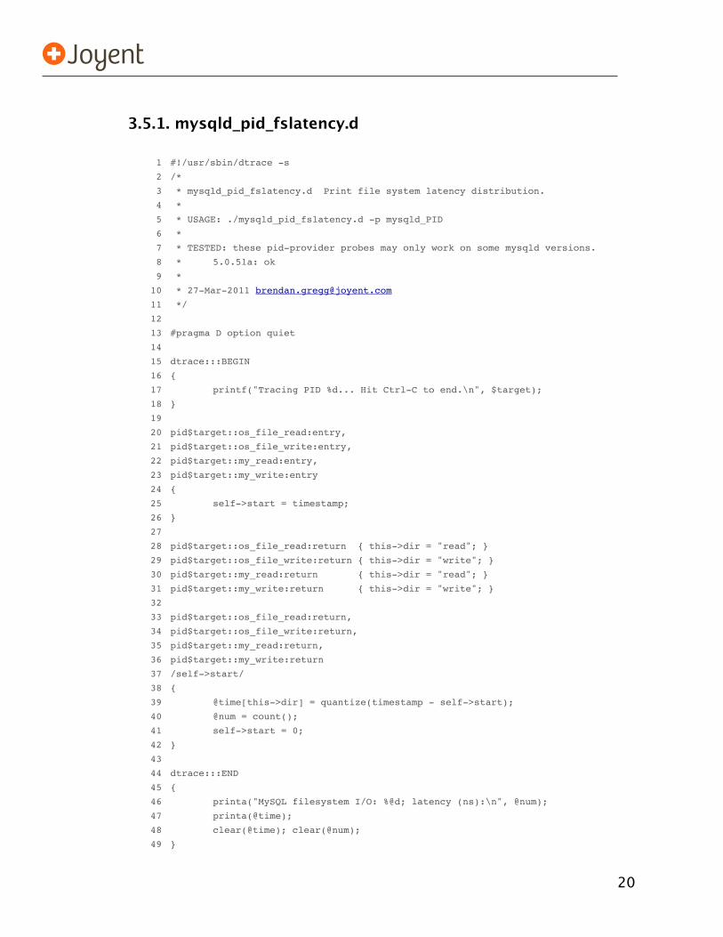
3.5. Distribution Script
The previous example traced I/O inside the application using the DTrace pid provider, and printed out a distribution plot of the file system latency. The tool executed, mysqld_pid_fslatency.d, is a DTrace script about 50 lines long (including comments). I’ve included it here, enumerated:
20
3.5.1. mysqld_pid_fslatency.d
1! #!/usr/sbin/dtrace -s
2! /*
3! * mysqld_pid_fslatency.d Print file system latency distribution.
4! *
5! * USAGE: ./mysqld_pid_fslatency.d -p mysqld_PID
6! *
7! * TESTED: these pid-provider probes may only work on some mysqld versions.
8! *! 5.0.51a: ok
9! *
10! * [email protected]
11! */
12
13! #pragma D option quiet
14
15! dtrace:::BEGIN
16! {
17! ! printf("Tracing PID %d... Hit Ctrl-C to end.\n", $target);
18! }
19
20! pid$target::os_file_read:entry,
21! pid$target::os_file_write:entry,
22! pid$target::my_read:entry,
23! pid$target::my_write:entry
24! {
25! ! self->start = timestamp;
26! }
27
28! pid$target::os_file_read:return { this->dir = "read"; }
29! pid$target::os_file_write:return { this->dir = "write"; }
30! pid$target::my_read:return { this->dir = "read"; }
31! pid$target::my_write:return { this->dir = "write"; }
32
33! pid$target::os_file_read:return,
34! pid$target::os_file_write:return,
35! pid$target::my_read:return,
36! pid$target::my_write:return
37! /self->start/
38! {
39! ! @time[this->dir] = quantize(timestamp - self->start);
40! ! @num = count();
41! ! self->start = 0;
42! }
43
44! dtrace:::END
45! {
46! ! printa("MySQL filesystem I/O: %@d; latency (ns):\n", @num);
47! ! printa(@time);
48! ! clear(@time); clear(@num);
49! }
21
This script traces functions in the mysql and innodb source that perform reads and writes to the file system: os_file_read(), os_file_write(), my_read() and my_write(). These function points were found by briefly examining the source code to this version of MySQL (5.0.51a), and checked by using DTrace to show user-land stack back traces when a production server was calling the file system.
On later MySQL versions, including 5.5.13, the os_file_read() and os_file_write() functions were renamed to be os_file_read_func() and os_file_write_func(). The script above can be modified accordingly (lines 20, 21, 28, 29, 33, 34) to match this change, allowing it to trace these MySQL versions.
3.5.2. Script Caveats
Since this is pid provider-based, these functions are not considered a stable interface: this script may not work on other versions of MySQL. As just mentioned, later versions of MySQL renamed the os_file* functions, causing this script to need updating to match those changes. Function renames are easy to cope with, this could be much harder. Functions could be added or removed, or the purpose of existing functions altered.
Besides the stability of this script, other caveats are:
• Overhead: there will be additional overhead (extra CPU cycles) for DTrace to instrument MySQL and collect this data. This should be minimal, especially considering the code-path instrumented – file system I/O. See my post on pid provider overhead for more discussion on this type of overhead.
• CPU latency: the times measured by this script include CPU dispatcher queue latency.
I’ll explain that last note in more detail.
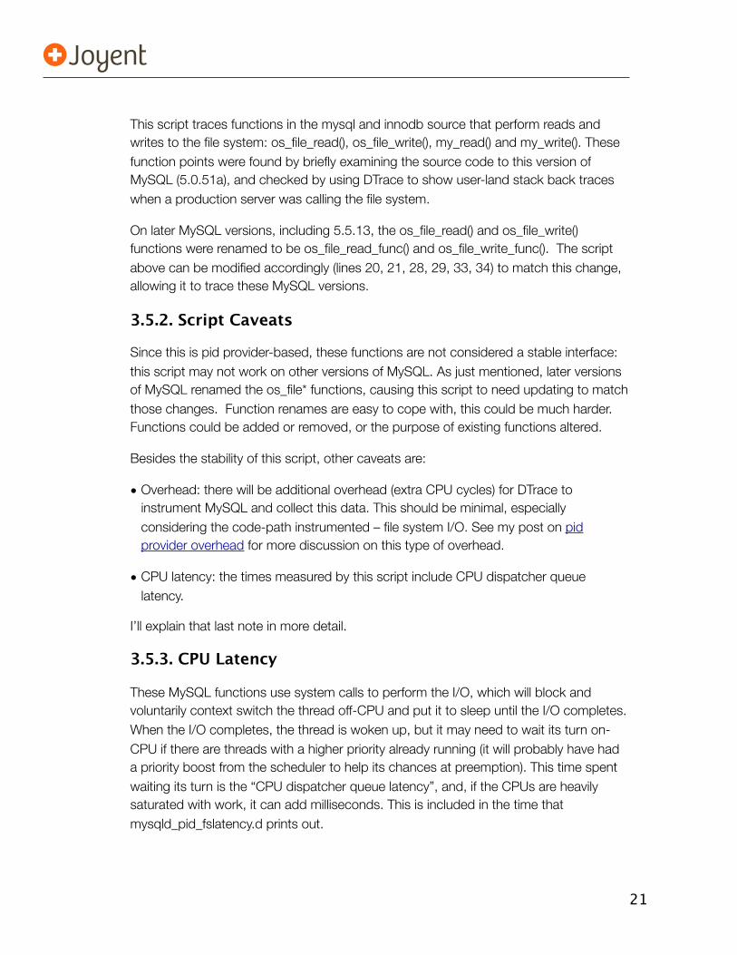
3.5.3. CPU Latency
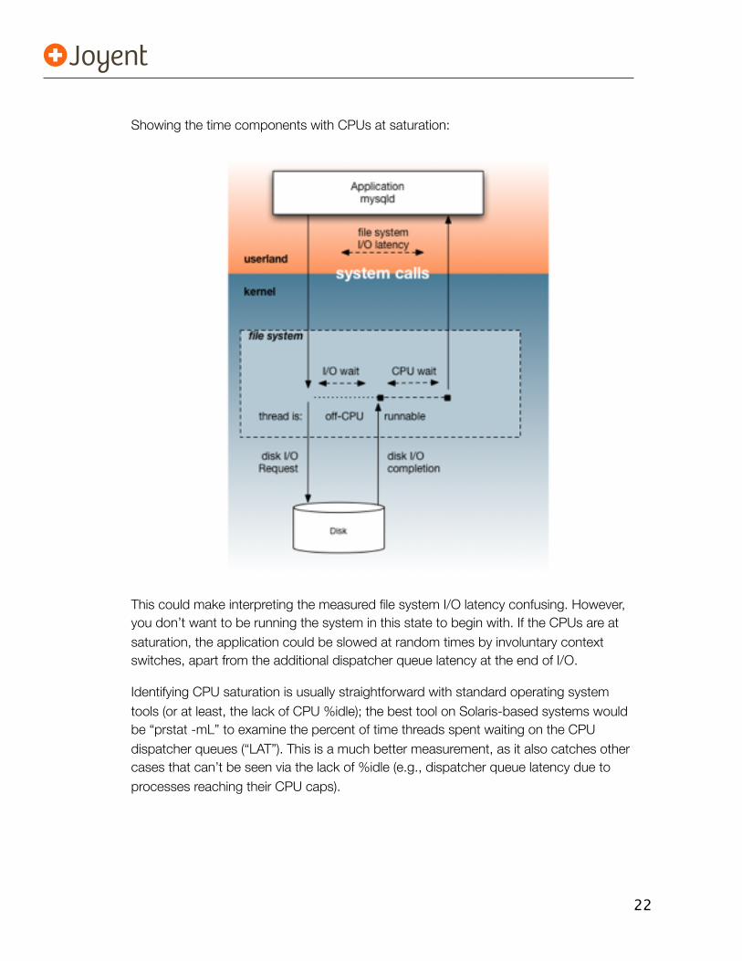
These MySQL functions use system calls to perform the I/O, which will block and voluntarily context switch the thread off-CPU and put it to sleep until the I/O completes. When the I/O completes, the thread is woken up, but it may need to wait its turn on-CPU if there are threads with a higher priority already running (it will probably have had a priority boost from the scheduler to help its chances at preemption). This time spent waiting its turn is the “CPU dispatcher queue latency”, and, if the CPUs are heavily saturated with work, it can add milliseconds. This is included in the time that mysqld_pid_fslatency.d prints out.
22
Showing the time components with CPUs at saturation:
This could make interpreting the measured file system I/O latency confusing. However, you don’t want to be running the system in this state to begin with. If the CPUs are at saturation, the application could be slowed at random times by involuntary context switches, apart from the additional dispatcher queue latency at the end of I/O.
Identifying CPU saturation is usually straightforward with standard operating system tools (or at least, the lack of CPU %idle); the best tool on Solaris-based systems would be “prstat -mL” to examine the percent of time threads spent waiting on the CPU dispatcher queues (“LAT”). This is a much better measurement, as it also catches other cases that can’t be seen via the lack of %idle (e.g., dispatcher queue latency due to processes reaching their CPU caps).
23
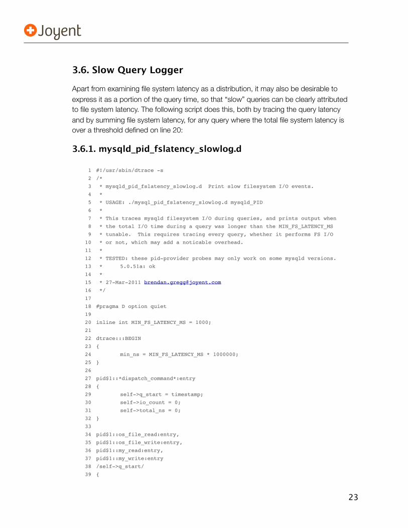
3.6. Slow Query Logger
Apart from examining file system latency as a distribution, it may also be desirable to express it as a portion of the query time, so that “slow” queries can be clearly attributed to file system latency. The following script does this, both by tracing the query latency and by summing file system latency, for any query where the total file system latency is over a threshold defined on line 20:
3.6.1. mysqld_pid_fslatency_slowlog.d
1! #!/usr/sbin/dtrace -s
2! /*
3! * mysqld_pid_fslatency_slowlog.d Print slow filesystem I/O events.
4! *
5! * USAGE: ./mysql_pid_fslatency_slowlog.d mysqld_PID
6! *
7! * This traces mysqld filesystem I/O during queries, and prints output when
8! * the total I/O time during a query was longer than the MIN_FS_LATENCY_MS
9! * tunable. This requires tracing every query, whether it performs FS I/O
10! * or not, which may add a noticable overhead.
11! *
12! * TESTED: these pid-provider probes may only work on some mysqld versions.
13! *! 5.0.51a: ok
14! *
15! * [email protected]
16! */
17
18! #pragma D option quiet
19
20! inline int MIN_FS_LATENCY_MS = 1000;
21
22! dtrace:::BEGIN
23! {
24! ! min_ns = MIN_FS_LATENCY_MS * 1000000;
25! }
26
27! pid$1::*dispatch_command*:entry
28! {
29! ! self->q_start = timestamp;
30! ! self->io_count = 0;
31! ! self->total_ns = 0;
32! }
33
34! pid$1::os_file_read:entry,
35! pid$1::os_file_write:entry,
36! pid$1::my_read:entry,
37! pid$1::my_write:entry
38! /self->q_start/
39! {
24
40! ! self->fs_start = timestamp;
41! }
42
43! pid$1::os_file_read:return,
44! pid$1::os_file_write:return,
45! pid$1::my_read:return,
46! pid$1::my_write:return
47! /self->fs_start/
48! {
49! ! self->total_ns += timestamp - self->fs_start;
50! ! self->io_count++;
51! ! self->fs_start = 0;
52! }
53
54! pid$1::*dispatch_command*:return
55! /self->q_start && (self->total_ns > min_ns)/
56! {
57! ! this->query = timestamp - self->q_start;
58! ! printf("%Y filesystem I/O during query > %d ms: ", walltimestamp,
59! ! MIN_FS_LATENCY_MS);
60! ! printf("query %d ms, fs %d ms, %d I/O\n", this->query / 1000000,
61! ! self->total_ns / 1000000, self->io_count);
62! }
63
64! pid$1::*dispatch_command*:return
65! /self->q_start/
66! {
67! ! self->q_start = 0;
68! ! self->io_count = 0;
69! ! self->total_ns = 0;
70! }
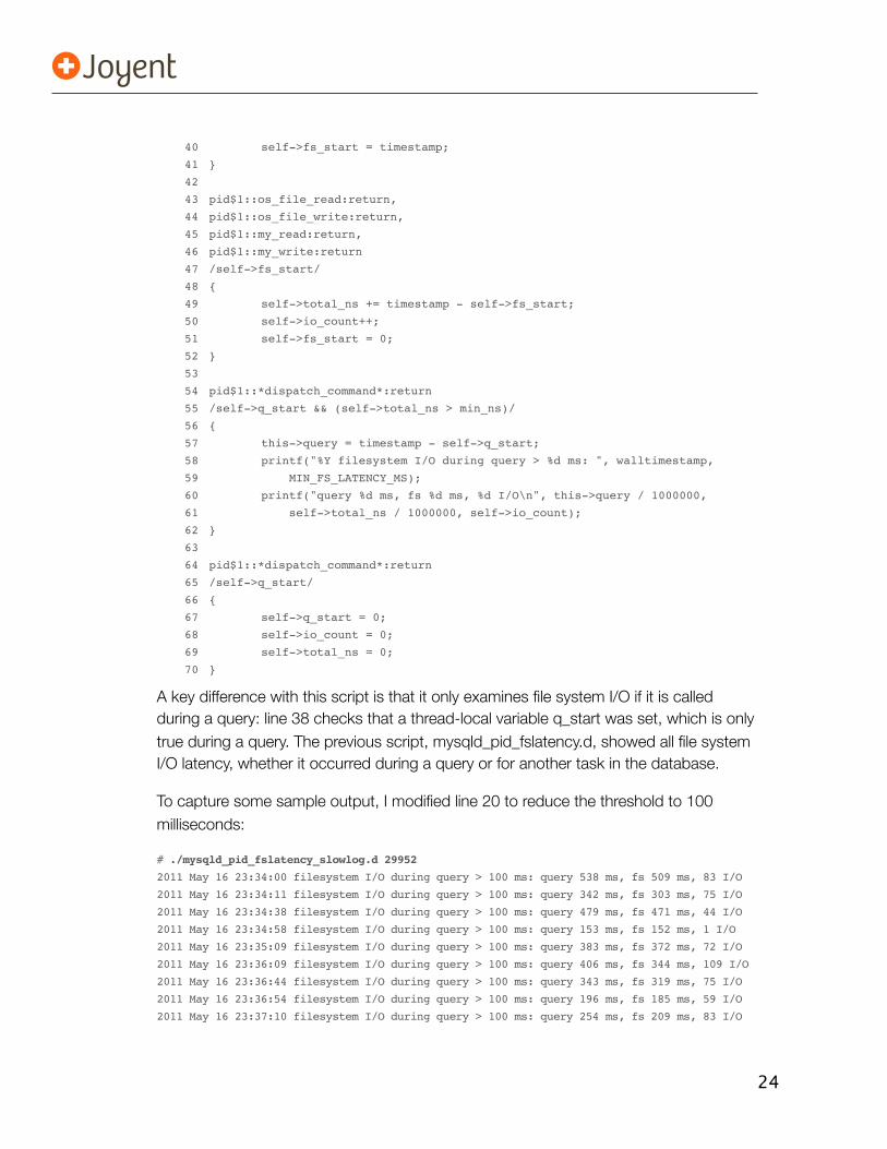
A key difference with this script is that it only examines file system I/O if it is called during a query: line 38 checks that a thread-local variable q_start was set, which is only true during a query. The previous script, mysqld_pid_fslatency.d, showed all file system I/O latency, whether it occurred during a query or for another task in the database.
To capture some sample output, I modified line 20 to reduce the threshold to 100 milliseconds:
# ./mysqld_pid_fslatency_slowlog.d 29952
2011 May 16 23:34:00 filesystem I/O during query > 100 ms: query 538 ms, fs 509 ms, 83 I/O
2011 May 16 23:34:11 filesystem I/O during query > 100 ms: query 342 ms, fs 303 ms, 75 I/O
2011 May 16 23:34:38 filesystem I/O during query > 100 ms: query 479 ms, fs 471 ms, 44 I/O
2011 May 16 23:34:58 filesystem I/O during query > 100 ms: query 153 ms, fs 152 ms, 1 I/O
2011 May 16 23:35:09 filesystem I/O during query > 100 ms: query 383 ms, fs 372 ms, 72 I/O
2011 May 16 23:36:09 filesystem I/O during query > 100 ms: query 406 ms, fs 344 ms, 109 I/O
2011 May 16 23:36:44 filesystem I/O during query > 100 ms: query 343 ms, fs 319 ms, 75 I/O
2011 May 16 23:36:54 filesystem I/O during query > 100 ms: query 196 ms, fs 185 ms, 59 I/O
2011 May 16 23:37:10 filesystem I/O during query > 100 ms: query 254 ms, fs 209 ms, 83 I/O
25
In the few minutes this was running, there were nine queries longer than 100 milliseconds due to file system I/O. With this output, we can immediately identify the reason for those slow queries: they spent most of their time waiting on the file system. Reaching this conclusion with other tools is much more difficult and time consuming – if possible (or practical) at all.
DTrace can be used to posiCvely idenCfy slow queries caused by file system latency.
But this is about more than DTrace; it’s about the metric itself: file system latency. Since this has been of tremendous use so far, it may make sense to add file system latency to the slow query log (requiring a MySQL source code change). If you are on MySQL 5.5 GA and later, you can get similar information from the wait/io events in the new performance schema additions. Mark Leith has demonstrated this in a post titled Monitoring MySQL IO Latency with performance_schema. If that isn’t viable, or you are on older MySQL, or a different application entirely (MySQL was just my example application), you can keep using DTrace to dynamically fetch this information.
3.6.2. Interpreting Totals
For the queries in the above output, most of the query latency is due to file system latency (e.g., 509 ms out of 538 ms = 95%). The last column printed out the I/O count, which helps answer the next question: is the file system latency due to many I/O operations, or a few slow ones? For example:
• The first line of output showed 509 milliseconds of file system latency from 83 I/O, which works out to about 6 milliseconds on average. Just based on the average, this could mean that most of these were cache misses causing random disk I/O. The next step may be to investigate the effect of doing fewer file system I/O in the first place, by caching more in MySQL.
• The fourth line of output shows 152 milliseconds of file system latency from a single I/O. This line of output is more alarming than any of the others, as it shows the file system returning with very high latency (this system is not at CPU saturation). Fortunately, this may be an isolated event.
If those descriptions sound a little vague, that’s because we’ve lost so much data when summarizing as an I/O count and a total latency. The script has achieved its goal of identifying the issue, but to investigate the issue further I need to return to the distribution plots like those used by mysqld_pid_fslatency.d. By examining the full distribution, I could confirm whether the 152 ms I/O was as isolated as it appears, or if in fact slow I/O is responsible for all of the latency seen above (e.g., for the first line, was it 3 slow I/O + 80 fast I/O = 83 I/O?).
26
3.6.3. Script Caveats
Caveats and notes for this script are:
• This script has a higher level of overhead than mysqld_pid_fslatency.d, since it is tracing all queries via the dispatch_command() function, not just file system functions.
• CPU latency: the file system time measured by this script includes CPU dispatcher queue latency (as explained earlier).
• The dispatch_command() function is matched as “*dispatch_command*”, since the full function name is the C++ signature (e.g., “_Z16dispatch_command19enum_server_commandP3THDPcj”, for this build of MySQL).
• Instead of using “-p PID” at the command line, this script fed in the PID as $1 (macro variable). I did this because this script is intended to be left running for hours, during which I may want to continue investigating MySQL with other DTrace programs. Only one “-p PID” script can be run at a time (“-p” locks the process, and other instances get the error “process is traced”). By using $1 for the long running script, shorter -p based ones can be run in the meantime.
A final note about these scripts: because they are pid provider-based, they can work from inside Solaris Zones or Joyent SmartMachines, with one minor caveat. When I executed the first script, I added “-n ‘tick-10s { exit(0); }’” at the command line to exit after 10 seconds. This currently does not work reliably in those environments due to a bug where the tick probe only fires sometimes. This was fixed in the recent release of SmartOS used by Joyent SmartMachines. If you are on an environment where this bug has not yet been fixed, drop that statement from the command line and it will still work fine, it will just require a Ctrl-C to end tracing.
3.7. Considering File System Latency
By examining latency at the file system level, we can immediately identify whether application issues are coming from the file system (and probably disk) or not. This starts us off at once down the right path, rather than in the wrong direction suggested by iostat(1M)’s view of busy disks.
Two pid provider-based DTrace scripts were introduced in this post to do this: mysqld_pid_fslatency.d for summarizing the distribution of file system latency, and mysqld_pid_fslatency_slowlog.d for printing slow queries due to the file system.

27
The pid provider isn’t the only way to measure file system latency: it’s also possible from the syscall layer and from the file system code in the kernel. I’ll demonstrate those methods in the next section, and discuss how they differ from the pid provider method.
28
4. Drilling Down Into the KernelPreviously I showed how to trace file system latency from within MySQL using the pid provider. Here I’ll show how similar data can be retrieved using the DTrace syscall and fbt providers. These allow us to trace at the system call layer, and deeper in the kernel at both the Virtual File System (VFS) interface and within the specific file system itself.
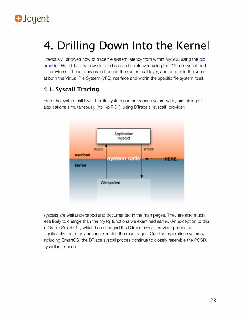
4.1. Syscall Tracing
From the system call layer, the file system can be traced system-wide, examining all applications simultaneously (no “-p PID”), using DTrace’s “syscall” provider:
syscalls are well understood and documented in the man pages. They are also much less likely to change than the mysql functions we examined earlier. (An exception to this is Oracle Solaris 11, which has changed the DTrace syscall provider probes so significantly that many no longer match the man pages. On other operating systems, including SmartOS, the DTrace syscall probes continue to closely resemble the POSIX syscall interface.)
29
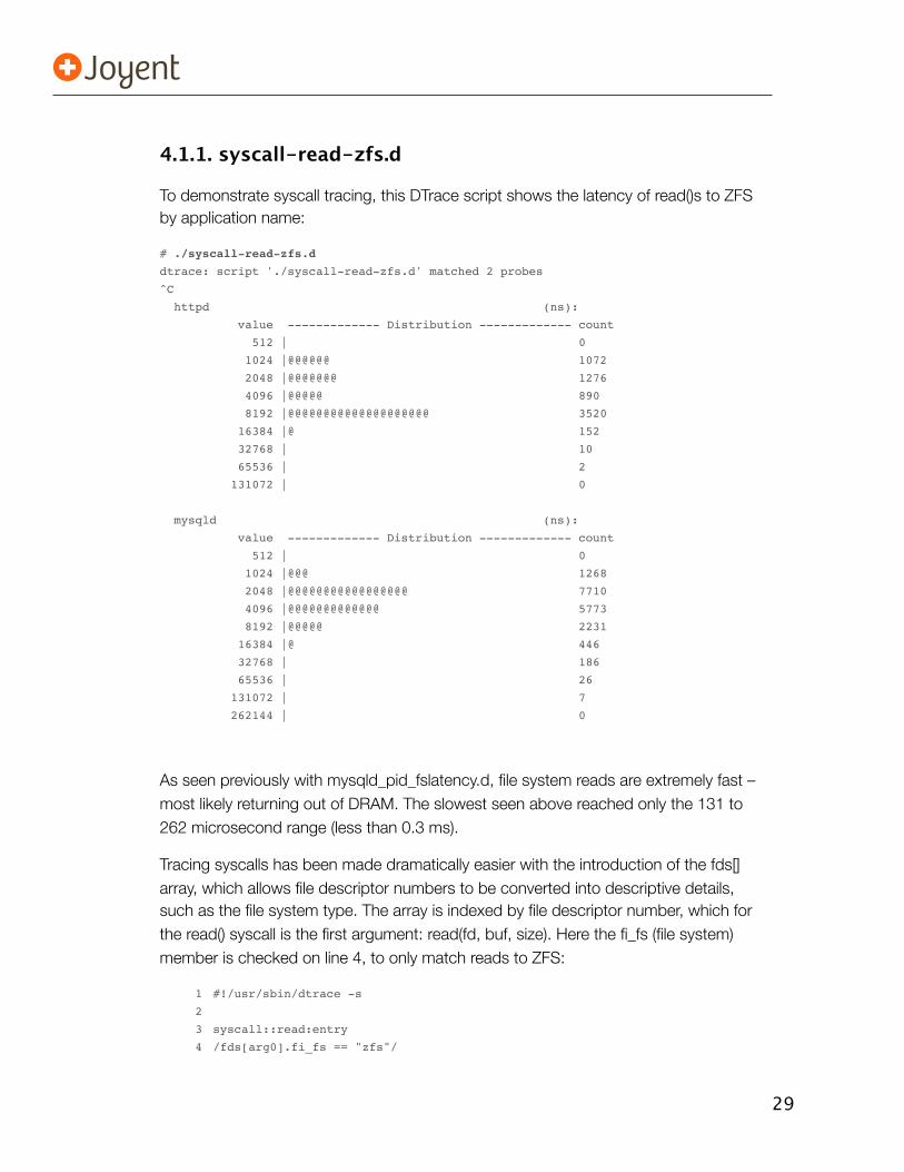
4.1.1. syscall-read-zfs.d
To demonstrate syscall tracing, this DTrace script shows the latency of read()s to ZFS by application name:
# ./syscall-read-zfs.d
dtrace: script './syscall-read-zfs.d' matched 2 probes
^C
httpd (ns):
value ------------- Distribution ------------- count
512 | 0
1024 |@@@@@@ 1072
2048 |@@@@@@@ 1276
4096 |@@@@@ 890
8192 |@@@@@@@@@@@@@@@@@@@@ 3520
16384 |@ 152
32768 | 10
65536 | 2
131072 | 0
mysqld (ns):
value ------------- Distribution ------------- count
512 | 0
1024 |@@@ 1268
2048 |@@@@@@@@@@@@@@@@@ 7710
4096 |@@@@@@@@@@@@@ 5773
8192 |@@@@@ 2231
16384 |@ 446
32768 | 186
65536 | 26
131072 | 7
262144 | 0
As seen previously with mysqld_pid_fslatency.d, file system reads are extremely fast – most likely returning out of DRAM. The slowest seen above reached only the 131 to 262 microsecond range (less than 0.3 ms).
Tracing syscalls has been made dramatically easier with the introduction of the fds[] array, which allows file descriptor numbers to be converted into descriptive details, such as the file system type. The array is indexed by file descriptor number, which for the read() syscall is the first argument: read(fd, buf, size). Here the fi_fs (file system) member is checked on line 4, to only match reads to ZFS:
1! #!/usr/sbin/dtrace -s
2
3! syscall::read:entry
4! /fds[arg0].fi_fs == "zfs"/
30
5! {
6! ! self->start = timestamp;
7! }
8
9! syscall::read:return
10! /self->start/
11! {
12! ! @[execname, "(ns):"] = quantize(timestamp - self->start);
13! ! self->start = 0;
14! }
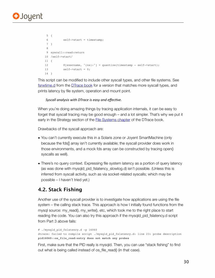
This script can be modified to include other syscall types, and other file systems. See fsrwtime.d from the DTrace book for a version that matches more syscall types, and prints latency by file system, operation and mount point.
Syscall analysis with DTrace is easy and effecCve.
When you’re doing amazing things by tracing application internals, it can be easy to forget that syscall tracing may be good enough – and a lot simpler. That’s why we put it early in the Strategy section of the File Systems chapter of the DTrace book.
Drawbacks of the syscall approach are:
• You can’t currently execute this in a Solaris zone or Joyent SmartMachine (only because the fds[] array isn’t currently available; the syscall provider does work in those environments, and a mock fds array can be constructed by tracing open() syscalls as well).
• There’s no query context. Expressing file system latency as a portion of query latency (as was done with mysqld_pid_fslatency_slowlog.d) isn’t possible. (Unless this is inferred from syscall activity, such as via socket-related syscalls; which may be possible – I haven’t tried yet.)
4.2. Stack Fishing
Another use of the syscall provider is to investigate how applications are using the file system – the calling stack trace. This approach is how I initially found functions from the mysql source: my_read(), my_write(), etc, which took me to the right place to start reading the code. You can also try this approach if the mysqld_pid_fslatency.d script from Part 3 above fails:
# ./mysqld_pid_fslatency.d -p 16060
dtrace: failed to compile script ./mysqld_pid_fslatency.d: line 23: probe description
pid16060::os_file_read:entry does not match any probes
First, make sure that the PID really is mysqld. Then, you can use “stack fishing” to find out what is being called instead of os_file_read() (in that case).
31
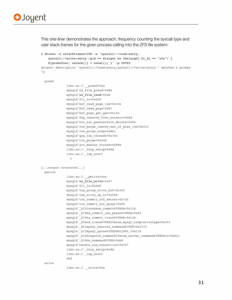
This one-liner demonstrates the approach, frequency counting the syscall type and user stack frames for the given process calling into the ZFS file system:
# dtrace -x ustackframes=100 -n 'syscall::*read:entry,
syscall::*write:entry /pid == $target && fds[arg0].fi_fs == "zfs"/ {
@[probefunc, ustack()] = count(); }' -p 29952
dtrace: description 'syscall::*read:entry,syscall::*write:entry ' matched 4 probes
^C
pread
libc.so.1`__pread+0xa
mysqld`os_file_pread+0x8e
mysqld`os_file_read+0x3b
mysqld`fil_io+0x2b0
mysqld`buf_read_page_low+0x14e
mysqld`buf_read_page+0x81
mysqld`buf_page_get_gen+0x143
mysqld`fsp_reserve_free_extents+0x6d
mysqld`btr_cur_pessimistic_delete+0x96
mysqld`row_purge_remove_sec_if_poss_low+0x31c
mysqld`row_purge_step+0x8e1
mysqld`que_run_threads+0x7c6
mysqld`trx_purge+0x3cb
mysqld`srv_master_thread+0x99d
libc.so.1`_thrp_setup+0x8d
libc.so.1`_lwp_start
1
[...output truncated...]
pwrite
libc.so.1`__pwrite+0xa
mysqld`os_file_write+0x97
mysqld`fil_io+0x2b0
mysqld`log_group_write_buf+0x34f
mysqld`log_write_up_to+0x566
mysqld`trx_commit_off_kernel+0x72f
mysqld`trx_commit_for_mysql+0x9f
mysqld`_Z15innobase_commitP3THDb+0x116
mysqld`_Z19ha_commit_one_phaseP3THDb+0x95
mysqld`_Z15ha_commit_transP3THDb+0x136
mysqld`_Z9end_transP3THD25enum_mysql_completiontype+0x191
mysqld`_Z21mysql_execute_commandP3THD+0x2172
mysqld`_Z11mysql_parseP3THDPKcjPS2_+0x116
mysqld`_Z16dispatch_command19enum_server_commandP3THDPcj+0xfc1
mysqld`_Z10do_commandP3THD+0xb8
mysqld`handle_one_connection+0x7f7
libc.so.1`_thrp_setup+0x8d
libc.so.1`_lwp_start
904
write
libc.so.1`__write+0xa
32
mysqld`my_write+0x3e
mysqld`my_b_flush_io_cache+0xdd
mysqld`_ZN9MYSQL_LOG14flush_and_syncEv+0x2a
mysqld`_ZN9MYSQL_LOG5writeEP3THDP11st_io_cacheP9Log_event+0x209
mysqld`_Z16binlog_end_transP3THDP11st_io_cacheP9Log_event+0x25
mysqld`_ZN9MYSQL_LOG7log_xidEP3THDy+0x51
mysqld`_Z15ha_commit_transP3THDb+0x24a
mysqld`_Z9end_transP3THD25enum_mysql_completiontype+0x191
mysqld`_Z21mysql_execute_commandP3THD+0x2172
mysqld`_Z11mysql_parseP3THDPKcjPS2_+0x116
mysqld`_Z16dispatch_command19enum_server_commandP3THDPcj+0xfc1
mysqld`_Z10do_commandP3THD+0xb8
mysqld`handle_one_connection+0x7f7
libc.so.1`_thrp_setup+0x8d
libc.so.1`_lwp_start
923
read
libc.so.1`__read+0xa
mysqld`my_read+0x4a
mysqld`_my_b_read+0x17d
mysqld`_ZN9Log_event14read_log_eventEP11st_io_cacheP6StringP14_pthread_mutex+0xf4
mysqld`_Z17mysql_binlog_sendP3THDPcyt+0x5dc
mysqld`_Z16dispatch_command19enum_server_commandP3THDPcj+0xc09
mysqld`_Z10do_commandP3THD+0xb8
mysqld`handle_one_connection+0x7f7
libc.so.1`_thrp_setup+0x8d
libc.so.1`_lwp_start
1496
read
libc.so.1`__read+0xa
mysqld`my_read+0x4a
mysqld`_my_b_read+0x17d
mysqld`_ZN9Log_event14read_log_eventEP11st_io_cacheP6StringP14_pthread_mutex+0xf4
mysqld`_Z17mysql_binlog_sendP3THDPcyt+0x35e
mysqld`_Z16dispatch_command19enum_server_commandP3THDPcj+0xc09
mysqld`_Z10do_commandP3THD+0xb8
mysqld`handle_one_connection+0x7f7
libc.so.1`_thrp_setup+0x8d
libc.so.1`_lwp_start
2939
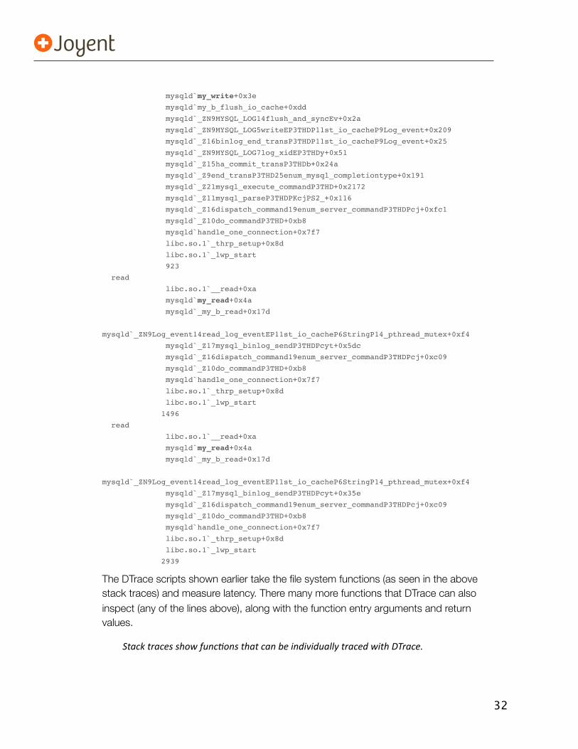
The DTrace scripts shown earlier take the file system functions (as seen in the above stack traces) and measure latency. There many more functions that DTrace can also inspect (any of the lines above), along with the function entry arguments and return values.
Stack traces show funcCons that can be individually traced with DTrace.
33
Note that this one-liner includes all file system I/O, not just those that occur during a query. The very first stack trace looks like an asynchronous database thread (srv_master_thread() -> trx_purge()), while all the rest appear to have occurred during a query (handle_one_connection() -> do_command()). The numbers at the bottom of the stack show the number of times entire stack trace was responsible for the syscall being called during tracing (I let it run for several seconds).
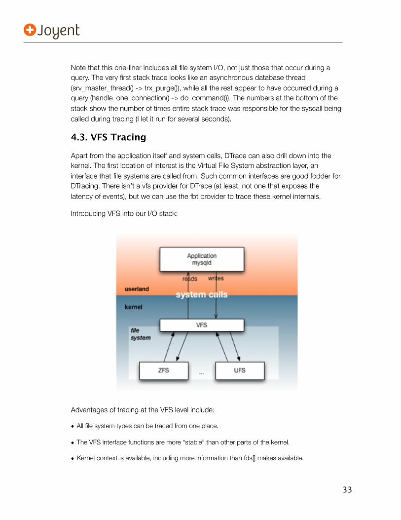
4.3. VFS Tracing
Apart from the application itself and system calls, DTrace can also drill down into the kernel. The first location of interest is the Virtual File System abstraction layer, an interface that file systems are called from. Such common interfaces are good fodder for DTracing. There isn’t a vfs provider for DTrace (at least, not one that exposes the latency of events), but we can use the fbt provider to trace these kernel internals.
Introducing VFS into our I/O stack:
Advantages of tracing at the VFS level include:
• All file system types can be traced from one place.
• The VFS interface functions are more “stable” than other parts of the kernel.
• Kernel context is available, including more information than fds[] makes available.
34
You can find examples of VFS tracing in Chapter 5 of the DTrace book, which can be downloaded as a sample chapter (PDF). Here is an example, solvfssnoop.d, which traces all VFS I/O on Solaris:
# ./solvfssnoop.d -n 'tick-10ms { exit(0); }'
TIME(ms) UID PID PROCESS CALL KB PATH
18844835237 104 29952 mysqld fop_read 0 <null>
18844835237 104 29952 mysqld fop_write 0 <null>
18844835238 0 22703 sshd fop_read 16 /devices/pseudo/clone@0:ptm
18844835237 104 29008 mysqld fop_write 16 /z01/opt/mysql5-64/data/xxxxx/
xxxxx.ibd
18844835237 104 29008 mysqld fop_write 32 /z01/opt/mysql5-64/data/xxxxx/
xxxxx.ibd
18844835237 104 29008 mysqld fop_write 48 /z01/opt/mysql5-64/data/xxxxx/
xxxxx.ibd
18844835237 104 29008 mysqld fop_write 16 /z01/opt/mysql5-64/data/xxxxx/
xxxxx.ibd
18844835237 104 29008 mysqld fop_write 16 /z01/opt/mysql5-64/data/xxxxx/
xxxxx.ibd
18844835237 104 29008 mysqld fop_write 32 /z01/opt/mysql5-64/data/xxxxx/
xxxxx.ibd
I’ve had to redact the filename info (replaced portions with “xxxxx”), but you should still get the picture. This has all the useful details except latency, which can be added to the script by tracing the “return” probe as well as the “entry” probes, and comparing timestamps (similar to how the syscalls were traced earlier). I’ll demonstrate this next with a simple one-liner.
Since VFS I/O can be very frequent (thousands of I/O per second), when I invoked the script above I added an action to exit after 10 milliseconds. The script also accepts a process name as an argument, e.g., “mysqld” to only trace VFS I/O from mysqld processes.
4.4. VFS Latency
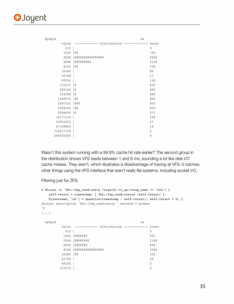
To demonstrate fetching latency info, here’s VFS read()s on Solaris traced via fop_read():
# dtrace -n 'fbt::fop_read:entry { self->start = timestamp; }
fbt::fop_read:return /self->start/ { @[execname, "ns"] =
quantize(timestamp - self->start); self->start = 0; }'
dtrace: description 'fbt::fop_read:entry ' matched 2 probes
^C
[...]
35
mysqld ns
value ------------- Distribution ------------- count
512 | 0
1024 |@@ 725
2048 |@@@@@@@@@@@@@@@@ 5928
4096 |@@@@@@@@@ 3319
8192 |@@ 708
16384 | 80
32768 | 17
65536 | 130
131072 |@ 532
262144 |@ 492
524288 |@ 489
1048576 |@@ 862
2097152 |@@@ 955
4194304 |@@ 602
8388608 |@ 271
16777216 | 102
33554432 | 27
67108864 | 14
134217728 | 2
268435456 | 0
Wasn’t this system running with a 99.9% cache hit rate earlier? The second group in the distribution shows VFS reads between 1 and 8 ms, sounding a lot like disk I/O cache misses. They aren’t, which illustrates a disadvantage of tracing at VFS: it catches other things using the VFS interface that aren’t really file systems, including socket I/O.
Filtering just for ZFS:
# dtrace -n 'fbt::fop_read:entry /args[0]->v_op->vnop_name == "zfs"/ {
self->start = timestamp; } fbt::fop_read:return /self->start/ {
@[execname, "ns"] = quantize(timestamp - self->start); self->start = 0; }'
dtrace: description 'fbt::fop_read:entry ' matched 2 probes
^C
[...]
mysqld ns
value ------------- Distribution ------------- count
512 | 0
1024 |@@@@@@@ 931
2048 |@@@@@@@@ 1149
4096 |@@@@@@@ 992
8192 |@@@@@@@@@@@@@@@@ 2266
16384 |@@ 320
32768 | 20
65536 | 2
131072 | 0
36
That’s better.
Drawbacks of VFS tracing:
• It can include other kernel components that use VFS, such as sockets.
• Application context is not available from VFS alone.
Drawbacks of VFS tracing using the fbt provider:
• It is not possible to use the fbt provider from Solaris zones or Joyent SmartMachines. It allows inspection of kernel internals, which has the potential to share privileged data between zones. It is therefore unlikely that the fbt provider will ever be available from within a zone. (There may be a way to do this securely, indirectly; more in part 5).
• The fbt provider is considered an “unstable” interface, since it exposes thousands of raw kernel functions. Any scripts written to use it may stop working on kernel updates, should the kernel engineer rename or modify functions you are tracing.
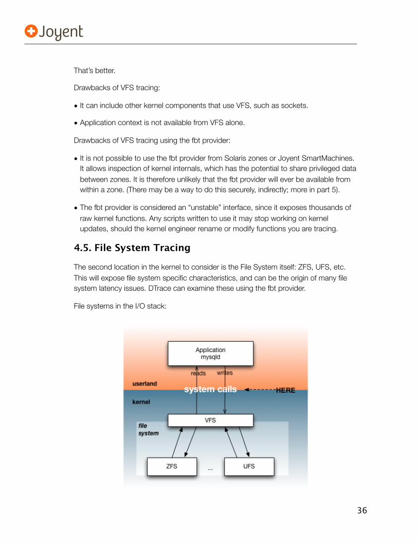
4.5. File System Tracing
The second location in the kernel to consider is the File System itself: ZFS, UFS, etc. This will expose file system specific characteristics, and can be the origin of many file system latency issues. DTrace can examine these using the fbt provider.
File systems in the I/O stack:
37
Advantages for tracing at the file system:
• File system specific behavior can be examined.
• Kernel context is available, including more information than fds[] makes available.
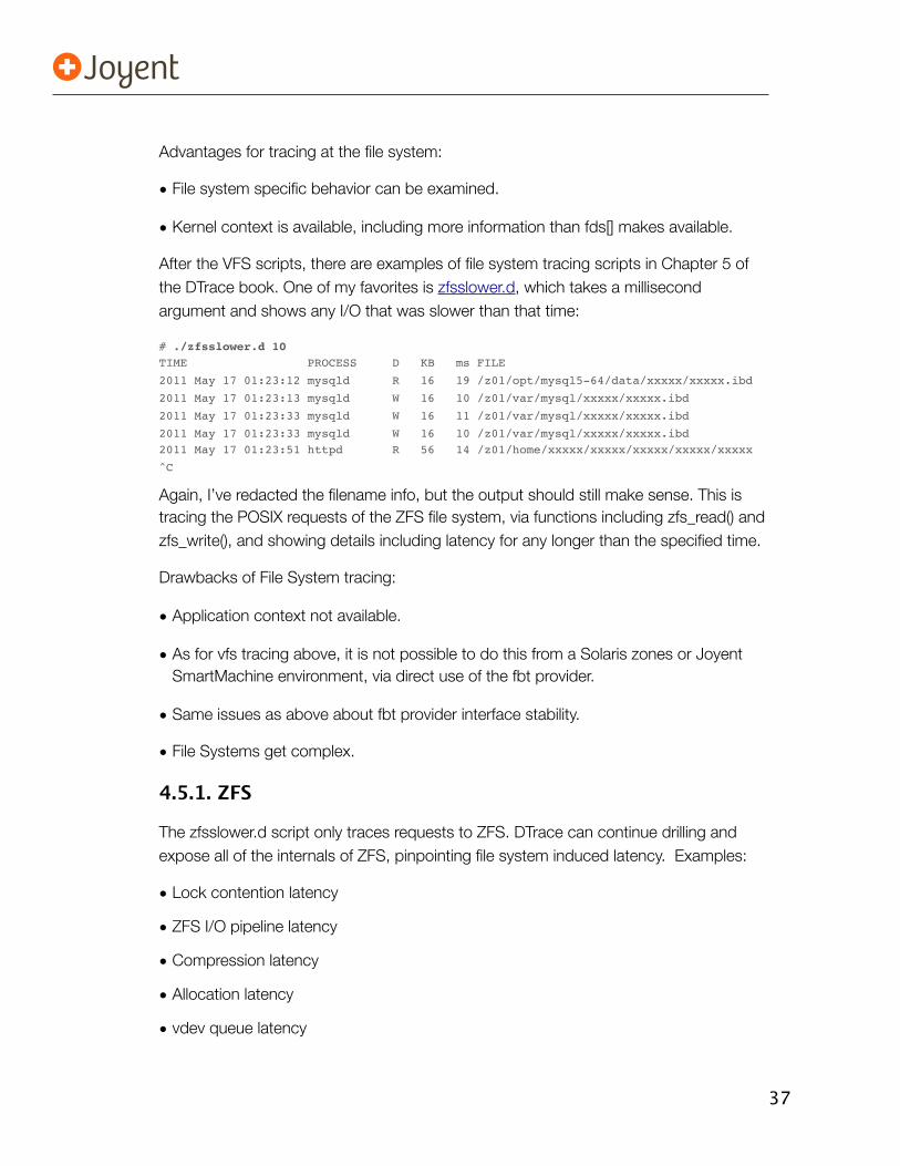
After the VFS scripts, there are examples of file system tracing scripts in Chapter 5 of the DTrace book. One of my favorites is zfsslower.d, which takes a millisecond argument and shows any I/O that was slower than that time:
# ./zfsslower.d 10 TIME PROCESS D KB ms FILE
2011 May 17 01:23:12 mysqld R 16 19 /z01/opt/mysql5-64/data/xxxxx/xxxxx.ibd
2011 May 17 01:23:13 mysqld W 16 10 /z01/var/mysql/xxxxx/xxxxx.ibd
2011 May 17 01:23:33 mysqld W 16 11 /z01/var/mysql/xxxxx/xxxxx.ibd
2011 May 17 01:23:33 mysqld W 16 10 /z01/var/mysql/xxxxx/xxxxx.ibd2011 May 17 01:23:51 httpd R 56 14 /z01/home/xxxxx/xxxxx/xxxxx/xxxxx/xxxxx
^C
Again, I’ve redacted the filename info, but the output should still make sense. This is tracing the POSIX requests of the ZFS file system, via functions including zfs_read() and zfs_write(), and showing details including latency for any longer than the specified time.
Drawbacks of File System tracing:
• Application context not available.
• As for vfs tracing above, it is not possible to do this from a Solaris zones or Joyent SmartMachine environment, via direct use of the fbt provider.
• Same issues as above about fbt provider interface stability.
• File Systems get complex.
4.5.1. ZFS
The zfsslower.d script only traces requests to ZFS. DTrace can continue drilling and expose all of the internals of ZFS, pinpointing file system induced latency. Examples:
• Lock contention latency
• ZFS I/O pipeline latency
• Compression latency
• Allocation latency
• vdev queue latency
38
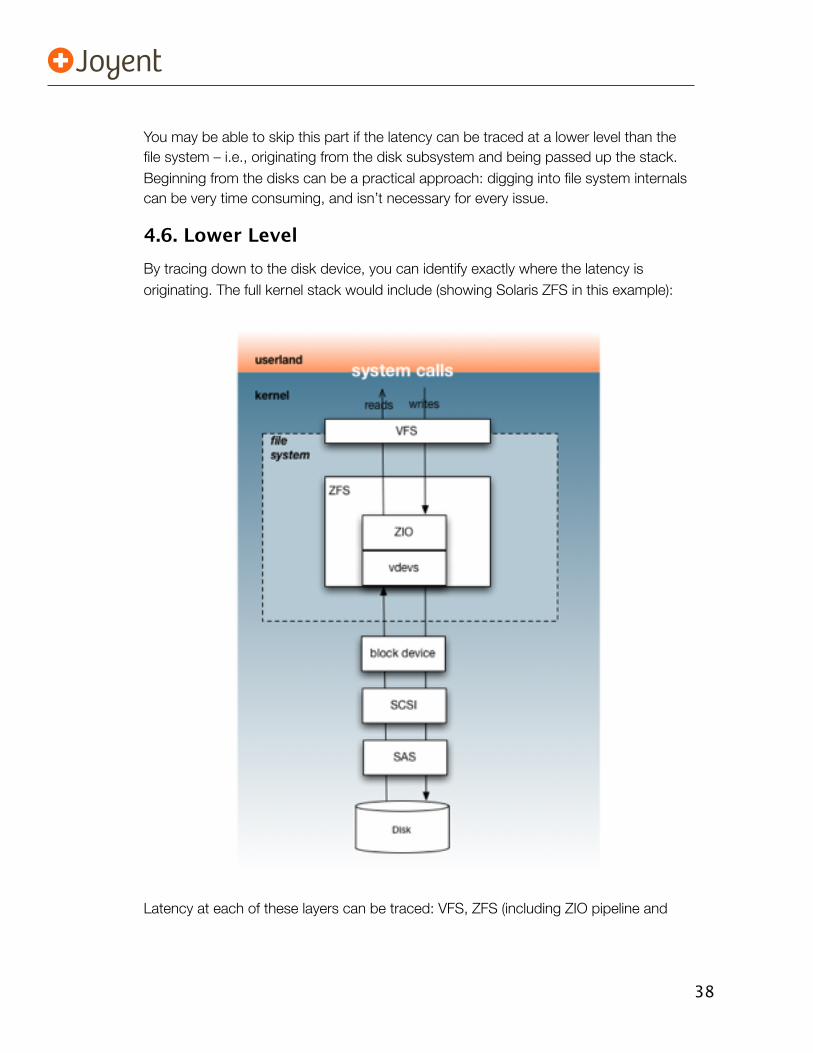
You may be able to skip this part if the latency can be traced at a lower level than the file system – i.e., originating from the disk subsystem and being passed up the stack. Beginning from the disks can be a practical approach: digging into file system internals can be very time consuming, and isn’t necessary for every issue.
4.6. Lower LevelBy tracing down to the disk device, you can identify exactly where the latency is originating. The full kernel stack would include (showing Solaris ZFS in this example):
Latency at each of these layers can be traced: VFS, ZFS (including ZIO pipeline and
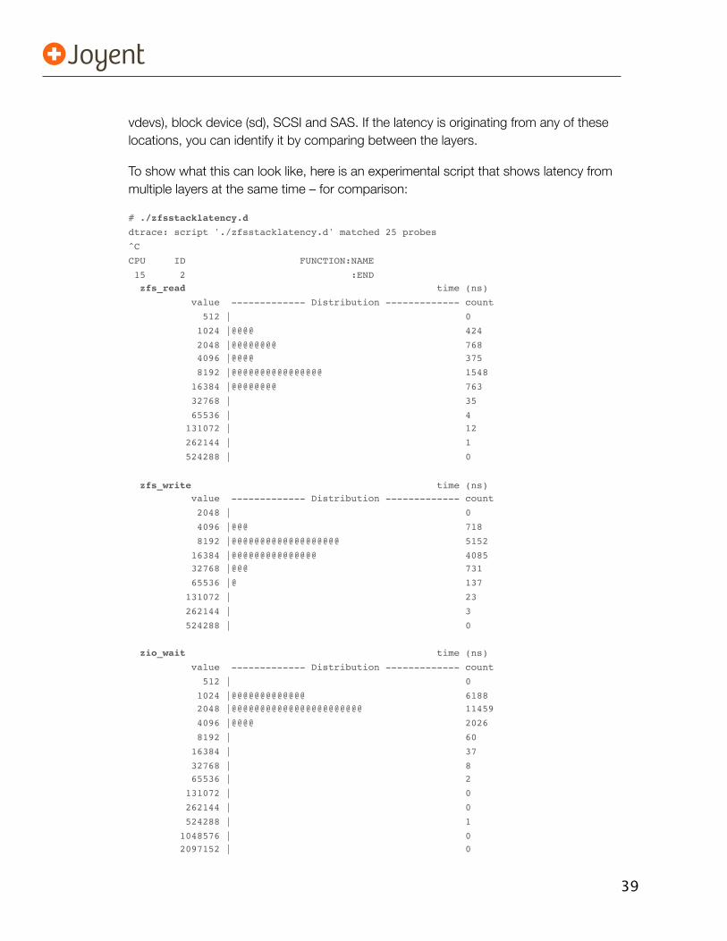
39
vdevs), block device (sd), SCSI and SAS. If the latency is originating from any of these locations, you can identify it by comparing between the layers.
To show what this can look like, here is an experimental script that shows latency from multiple layers at the same time – for comparison:
# ./zfsstacklatency.d
dtrace: script './zfsstacklatency.d' matched 25 probes
^C
CPU ID FUNCTION:NAME
15 2 :END zfs_read time (ns)
value ------------- Distribution ------------- count
512 | 0
1024 |@@@@ 424
2048 |@@@@@@@@ 768 4096 |@@@@ 375
8192 |@@@@@@@@@@@@@@@@ 1548
16384 |@@@@@@@@ 763
32768 | 35
65536 | 4 131072 | 12
262144 | 1
524288 | 0
zfs_write time (ns) value ------------- Distribution ------------- count
2048 | 0
4096 |@@@ 718
8192 |@@@@@@@@@@@@@@@@@@@ 5152
16384 |@@@@@@@@@@@@@@@ 4085 32768 |@@@ 731
65536 |@ 137
131072 | 23
262144 | 3
524288 | 0
zio_wait time (ns)
value ------------- Distribution ------------- count
512 | 0
1024 |@@@@@@@@@@@@@ 6188 2048 |@@@@@@@@@@@@@@@@@@@@@@@ 11459
4096 |@@@@ 2026
8192 | 60
16384 | 37
32768 | 8 65536 | 2
131072 | 0
262144 | 0
524288 | 1
1048576 | 0 2097152 | 0
40
4194304 | 0
8388608 | 0
16777216 | 0 33554432 | 0
67108864 | 0
134217728 | 0
268435456 | 1
536870912 | 0
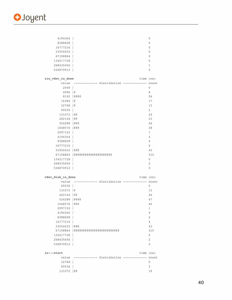
zio_vdev_io_done time (ns)
value ------------- Distribution ------------- count
2048 | 0
4096 |@ 8 8192 |@@@@ 56
16384 |@ 17
32768 |@ 13
65536 | 2
131072 |@@ 24 262144 |@@ 23
524288 |@@@ 44
1048576 |@@@ 38
2097152 | 1
4194304 | 4 8388608 | 4
16777216 | 4
33554432 |@@@ 43
67108864 |@@@@@@@@@@@@@@@@@@@@@ 315
134217728 | 0 268435456 | 2
536870912 | 0
vdev_disk_io_done time (ns)
value ------------- Distribution ------------- count 65536 | 0
131072 |@ 12
262144 |@@ 26
524288 |@@@@ 47
1048576 |@@@ 40 2097152 | 1
4194304 | 4
8388608 | 4
16777216 | 4
33554432 |@@@ 43 67108864 |@@@@@@@@@@@@@@@@@@@@@@@@@ 315
134217728 | 0
268435456 | 2
536870912 | 0
io:::start time (ns)
value ------------- Distribution ------------- count
32768 | 0
65536 | 3
131072 |@@ 19
41
262144 |@@ 21
524288 |@@@@ 45
1048576 |@@@ 38 2097152 | 0
4194304 | 4
8388608 | 4
16777216 | 4
33554432 |@@@ 43 67108864 |@@@@@@@@@@@@@@@@@@@@@@@@@ 315
134217728 | 0
268435456 | 2
536870912 | 0
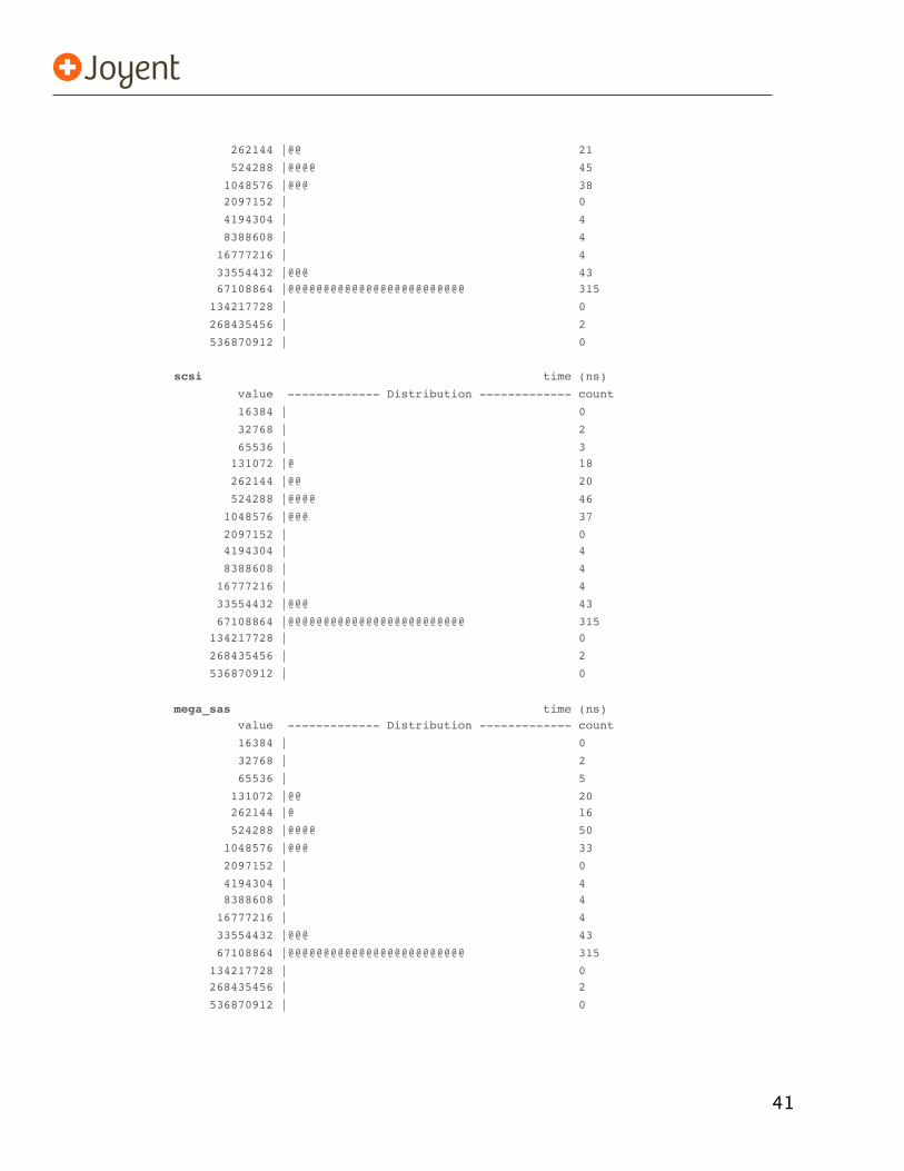
scsi time (ns)
value ------------- Distribution ------------- count
16384 | 0
32768 | 2
65536 | 3 131072 |@ 18
262144 |@@ 20
524288 |@@@@ 46
1048576 |@@@ 37
2097152 | 0 4194304 | 4
8388608 | 4
16777216 | 4
33554432 |@@@ 43
67108864 |@@@@@@@@@@@@@@@@@@@@@@@@@ 315 134217728 | 0
268435456 | 2
536870912 | 0
mega_sas time (ns) value ------------- Distribution ------------- count
16384 | 0
32768 | 2
65536 | 5
131072 |@@ 20 262144 |@ 16
524288 |@@@@ 50
1048576 |@@@ 33
2097152 | 0
4194304 | 4 8388608 | 4
16777216 | 4
33554432 |@@@ 43
67108864 |@@@@@@@@@@@@@@@@@@@@@@@@@ 315
134217728 | 0 268435456 | 2
536870912 | 0
42
mega_sas is the SAS disk device driver – which shows the true latency of the disk I/O (about as deep as the operating system can go). The first distribution printed was for zfs_read() latency, which are the read requests to ZFS.
It’s hugely valuable to be able to pluck this sort of latency data out from different layers of the operating system stack, to narrow down the source of the latency. Comparing all I/O in this way can also identify the origin of outliers (a few I/O with high latency) quickly, which may be hit-or-miss if single I/O were picked and traced as they executed through the kernel.
Latency at different levels of the OS stack can be examined and compared to idenCfy the origin.
The spike of slow disk I/O seen in the mega_sas distribution (315 I/O with a latency between 67 and 134 ms), which is likely due to queueing on the disk, propagates up the stack to a point and then vanishes. That latency is not visible in the zfs_read() and zfs_write() interfaces, meaning that no application was affected by that latency (at least via read/write). The spike corresponded to a ZFS TXG flush – which is asynchronous to the application, and queues a bunch of I/O to the disks. If that spike were to propagate all the way up into zfs_read()/zfs_write(), then this output would have identified the origin: the disks.
4.6.1. zfsstacklatency.d
I wrote zfsstacklatency.d as a demonstration script, to show what is technically possible. The script breaks a rule that I learned the hard way: keep it simple. zfsstacklatency.d is not simple, it traces at multiple stack layers using the unstable fbt provider and is over 100 lines long. This makes it brittle and not likely to run on different kernel builds other than the system I’m on (there is little point including it here, since it almost certainly won’t run for you). To trace at these layers, it can be more reliable to run small scripts that trace individual layers separately, and to maintain those individual scripts if and when they break on newer kernel versions. Chapter 4 of the DTrace book does this via scripts such as scsilatency.d, satalatency.d, mptlatency.d, etc.
4.7. Comparing File System Latency
By examining latency at different levels of the I/O stack, its origin can be identified. DTrace provides the ability to trace latency from the application right down to the disk device driver, leaving no stone unturned. This can be especially useful for the cases where latency is not caused by the disks, but by other issues in the kernel.
In the final section, I’ll show other useful presentations of file system latency as a metric.
43
5. Presenting File System LatencyI previously explained why disk I/O metrics may not reflect application performance, and how some file system issues may be invisible at the disk I/O level. I then showed how to resolve this by measuring file system latency at the application level using MySQL as an example, and measured latency from other levels of the operating system stack to pinpoint the origin.
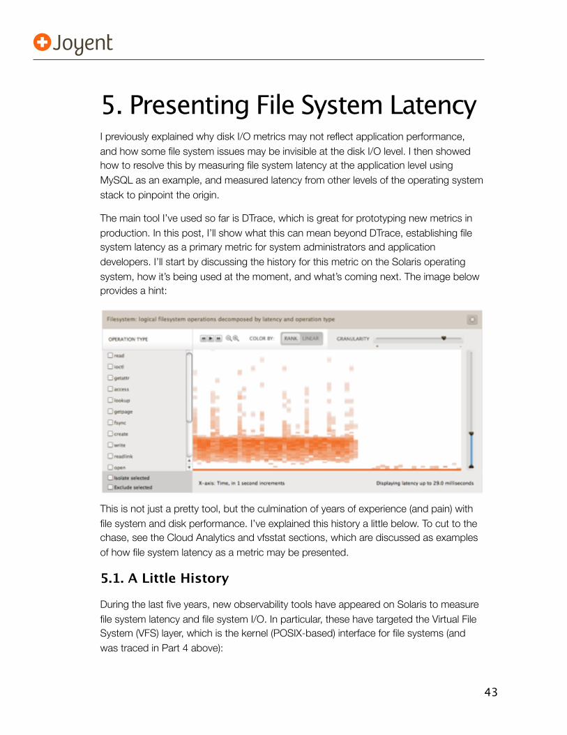
The main tool I’ve used so far is DTrace, which is great for prototyping new metrics in production. In this post, I’ll show what this can mean beyond DTrace, establishing file system latency as a primary metric for system administrators and application developers. I’ll start by discussing the history for this metric on the Solaris operating system, how it’s being used at the moment, and what’s coming next. The image below provides a hint:
This is not just a pretty tool, but the culmination of years of experience (and pain) with file system and disk performance. I’ve explained this history a little below. To cut to the chase, see the Cloud Analytics and vfsstat sections, which are discussed as examples of how file system latency as a metric may be presented.
5.1. A Little History
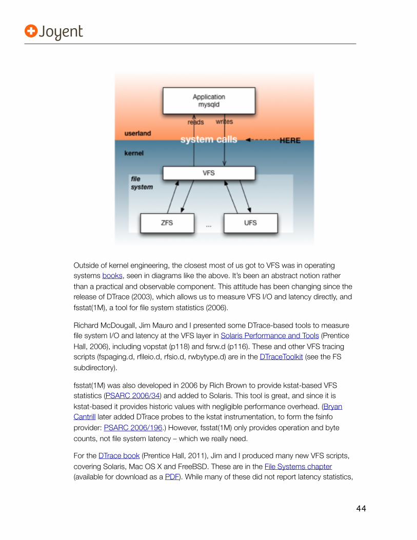
During the last five years, new observability tools have appeared on Solaris to measure file system latency and file system I/O. In particular, these have targeted the Virtual File System (VFS) layer, which is the kernel (POSIX-based) interface for file systems (and was traced in Part 4 above):
44
Outside of kernel engineering, the closest most of us got to VFS was in operating systems books, seen in diagrams like the above. It’s been an abstract notion rather than a practical and observable component. This attitude has been changing since the release of DTrace (2003), which allows us to measure VFS I/O and latency directly, and fsstat(1M), a tool for file system statistics (2006).
Richard McDougall, Jim Mauro and I presented some DTrace-based tools to measure file system I/O and latency at the VFS layer in Solaris Performance and Tools (Prentice Hall, 2006), including vopstat (p118) and fsrw.d (p116). These and other VFS tracing scripts (fspaging.d, rfileio.d, rfsio.d, rwbytype.d) are in the DTraceToolkit (see the FS subdirectory).
fsstat(1M) was also developed in 2006 by Rich Brown to provide kstat-based VFS statistics (PSARC 2006/34) and added to Solaris. This tool is great, and since it is kstat-based it provides historic values with negligible performance overhead. (Bryan Cantrill later added DTrace probes to the kstat instrumentation, to form the fsinfo provider: PSARC 2006/196.) However, fsstat(1M) only provides operation and byte counts, not file system latency – which we really need.
For the DTrace book (Prentice Hall, 2011), Jim and I produced many new VFS scripts, covering Solaris, Mac OS X and FreeBSD. These are in the File Systems chapter (available for download as a PDF). While many of these did not report latency statistics,
45
it is not difficult to enhance the scripts to do so, tracing the time between the “entry” and “return” probes (as was demonstrated via a one-liner in part 4).
DTrace has been the most practical way to measure file system latency across arbitrary applications, especially scripts like those in part 3. I’ll comment briefly on a few more sources of performance metrics, mostly from Solaris-based systems: kstats, truss(1M), LatencyTOP, SystemTap (Linux), and application instrumentation.
5.1.1. kstats
Kernel statistics (kstats) is a “registry of metrics” (thanks to Ben Rockwood for the term) on Solaris, which provide the raw numbers for traditional observability tools including iostat(1M). While there are many thousands of kstats available, file system latency was not among them.
Even if you are a vendor whose job it is to build monitoring tools on top of Solaris, you can only use what the operating system gives you, hence the focus on disk I/O statistics from iostat(1M) or kstat. More on this in a moment (vfsstat).
5.1.2. truss, strace
You could attach system call tracers such as truss(1) or strace(1) to applications one by one to get latency from the syscall level. This would involve examining reads and writes and associating them back to file system-based file descriptors, along with timing data. However, the overhead of these tools is often prohibitive in production due to the way they work.
5.1.3. LatencyTOP
Another tool that could measure file system latency is LatencyTOP. This was released in 2008 by Intel to identify sources of desktop latency on Linux, and implemented by the addition of static trace points throughout the kernel. To see if DTrace could fetch similar data without kernel changes, I quickly wrote latencytop.d. LatencyTOP itself was ported to Solaris in 2009 (PSARC 2009/339):
LatencyTOP uses the Solaris DTrace APIs, specifically the following DTrace providers: sched, proc and lockstat.
While it isn’t a VFS or file system oriented tool, its latency statistics do include file system read and write latency, presenting them as a “Maximum” and “Average”. With these, it may be possible to identify instances of high latency (outliers), and increased average latency. Which is handy, but about all that is possible. To confirm that file
46
system latency is directly causing slow queries, you’ll need to use more DTrace, as I did in part 3 above, to sum file system latency during query latency.
5.1.4. SystemTap
For Linux systems, I developed a SystemTap-based tool to measure VFS read latency and show the file system type: vfsrlat.stp. This allows ext4 read latency to be examined in detail, showing distribution plots of latency. I expect to continue to use vfsrlat.stp and others I’ve written, in Linux lab environments, until one of the ports of DTrace to Linux is sufficiently complete to use.
5.1.5. Applications
Application developers can instrument their code as it performs file I/O, collecting high resolution timestamps to calculate file system latency metrics1. Because of this, they haven’t needed DTrace - but they do need the foresight to have added these metrics before the application is in production. Too often I’ve been looking at a system where if we could restart the application with different options, we could probably get the perfor-mance data needed. But restarting the application comes with serious cost (downtime), and can mean that the performance issue isn’t visible again for hours or days (e.g., memory growth/leak related). DTrace can provide the required data immediately.
DTrace isn’t better than application-level metrics. If the application already provides file system latency metrics, use them. Running DTrace will add much more performance overhead than (well designed) application-level counters.
Check what the applicaCon provides before turning to DTrace.
I put this high up in the Strategy sections in the DTrace book, not only to avoid re-inventing the wheel, but because familiarization with application metrics is excellent context to build upon with DTrace.
5.1.6. MySQL
I’ve been using MySQL as an example application to investigate, and introduced DTrace-based tools to illustrate the techniques. While not the primary objective of this white paper, these tools are of immediate practical use for MySQL, and have been successfully employed during performance investigations on the Joyent public cloud.
1 Well, almost. See the “CPU Latency” section in Part 3, which is also true for application-level measurements. DTrace can inspect the kernel and differentiate CPU latency from file system latency, but as I said in part 3, you don’t want to be running in a CPU latency state to start with.
47
Recent versions of MySQL have provided the performance schema which can measure file system latency, without needing to use DTrace. Mark Leith posted a detailed article: Monitoring MySQL IO Latency with performance_schema, writing:
filesystem latency can be monitored from the current MySQL 5.5 GA version, with performance schema, on all plaWorms.
This is good news if you are on MySQL 5.5 GA or later, and are running with the performance-schema option.
The DTrace story doesn’t quite end here. DTrace can leverage and extend the performance schema by tracing its functions along with additional information.
5.2. What’s Happening Now
I regular use DTrace to identify issues of high file system latency, and to quantify how much it is affecting application performance. This is for cloud computing environments, where multiple tenants are sharing a pool of disks, and where disk I/O statistics from iostat(1M) look more alarming than reality (reasons why this can happen are explained in Part 1).
The most useful scripts I’m using include those I showed in Part 3 to measure latency from within MySQL; these can be run by the customer. Most of the time they show that the file system is performing well, and returning out of DRAM cache (thanks to our environment). This leads the investigation to other areas, narrowing the scope to where the issue really is, and not wasting time where it isn’t.
I’ve also identified real disk based issues (which are fortunately rare) which, when traced as file system latency, show that the application really is affected. Again, this saves time: knowing for sure that there is a file system issue to investigate is much better than guessing that there might be one.
Tracing file system latency has worked best from two locations:
Application layer: as demonstrated in Part 3 above, this provides application context to identify whether the issue is real (synchronous to workload) and what is affected (workload attributes). The key example was mysqld_pid_fslatency_slowlog.d, which printed the total file system latency along with the query latency, so that slow queries could be immediately identified as file system-based or not.
VFS layer: as demonstrated in Part 4, this allows all applications to be traced simultaneously regardless of their I/O code path. Since these trace inside the kernel,
48
the scripts cannot be run by customers in the cloud computing environment (zones), as the fbt provider is not available to them (for security reasons).
For the rare times that there is high file system latency, I’ll dig down deeper into the kernel stack to pinpoint the location, tracing the specific file system type (ZFS, UFS, …), and disk device drivers, as shown in Part 4 and in chapters 4 and 5 of the DTrace book. This includes using several custom fbt provider-based DTrace scripts, which are fairly brittle as they trace a specific kernel version.
5.3. What’s Next
File system latency has become so important that examining it interactively via DTrace scripts is not enough. Many people do use remote monitoring tools (e.g., munin) to fetch statistics for graphing, and it’s not straightforward to run these DTrace scripts 24×7 to feed remote monitoring. Nor is it straightforward to take the latency distribution plots that DTrace can provide and graph them using standard tools.
At Joyent we’ve been developing solutions to these in the latest version of our operating system, SmartOS (based on Illumos) and in our SmartDataCenter product. These include vfsstat(1M) and the file system latency heat maps in Cloud Analytics.
5.4. vfsstat(1M)For a disk I/O summary, iostat(1M) does do a good job (using -x for the extended columns). The limitation is that, from an application perspective, we’d like the statistics to be measured closer to the app, such as in the VFS level.
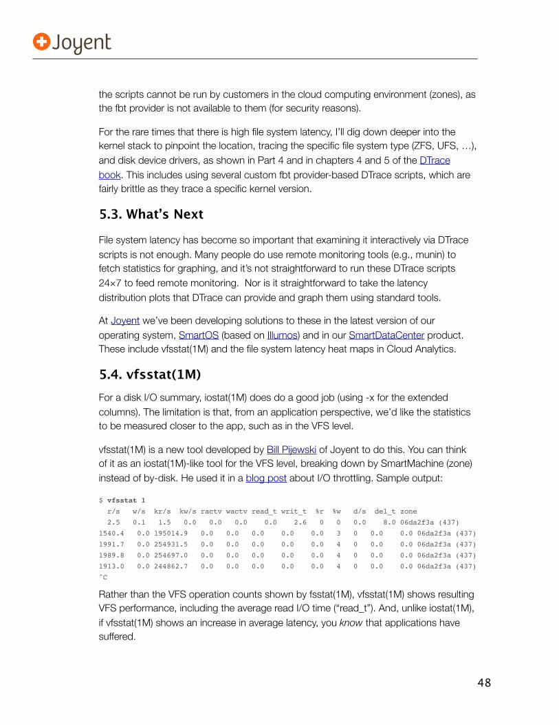
vfsstat(1M) is a new tool developed by Bill Pijewski of Joyent to do this. You can think of it as an iostat(1M)-like tool for the VFS level, breaking down by SmartMachine (zone) instead of by-disk. He used it in a blog post about I/O throttling. Sample output:
$ vfsstat 1
r/s w/s kr/s kw/s ractv wactv read_t writ_t %r %w d/s del_t zone
2.5 0.1 1.5 0.0 0.0 0.0 0.0 2.6 0 0 0.0 8.0 06da2f3a (437)
1540.4 0.0 195014.9 0.0 0.0 0.0 0.0 0.0 3 0 0.0 0.0 06da2f3a (437)
1991.7 0.0 254931.5 0.0 0.0 0.0 0.0 0.0 4 0 0.0 0.0 06da2f3a (437)
1989.8 0.0 254697.0 0.0 0.0 0.0 0.0 0.0 4 0 0.0 0.0 06da2f3a (437)
1913.0 0.0 244862.7 0.0 0.0 0.0 0.0 0.0 4 0 0.0 0.0 06da2f3a (437)
^C
Rather than the VFS operation counts shown by fsstat(1M), vfsstat(1M) shows resulting VFS performance, including the average read I/O time (“read_t”). And, unlike iostat(1M), if vfsstat(1M) shows an increase in average latency, you know that applications have suffered.
49
If vfsstat(1M) does identify high latency, the next question is to check whether sensitive code-paths have suffered (the “synchronous component of the workload” requirement), which can be identified using the pid provider. An example of this was the mysqld_pid_fslatency_slowlog.d script in Part 3, which expressed total file system I/O latency next to query time.
vfsstat(1M) can be a handy tool to run before reaching for DTrace, as it is using kernel statistics (kstats) that are essentially free to use (already maintained and active). The tool can also be run as a non-root user.
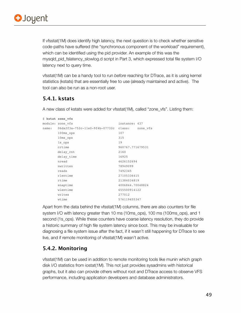
5.4.1. kstats
A new class of kstats were added for vfsstat(1M), called “zone_vfs”. Listing them:
$ kstat zone_vfs
module: zone_vfs instance: 437
name: 06da2f3a-752c-11e0-9f4b-07732c class: zone_vfs
100ms_ops 107
10ms_ops 315
1s_ops 19
crtime 960767.771679531
delay_cnt 2160
delay_time 16925
nread 4626152694
nwritten 78949099
reads 7492345
rlentime 27105336415
rtime 21384034819
snaptime 4006844.70048824
wlentime 655500914122
writes 277012
wtime 576119455347
Apart from the data behind the vfsstat(1M) columns, there are also counters for file system I/O with latency greater than 10 ms (10ms_ops), 100 ms (100ms_ops), and 1 second (1s_ops). While these counters have coarse latency resolution, they do provide a historic summary of high file system latency since boot. This may be invaluable for diagnosing a file system issue after the fact, if it wasn’t still happening for DTrace to see live, and if remote monitoring of vfsstat(1M) wasn’t active.
5.4.2. Monitoring
vfsstat(1M) can be used in addition to remote monitoring tools like munin which graph disk I/O statistics from iostat(1M). This not just provides sysadmins with historical graphs, but it also can provide others without root and DTrace access to observe VFS performance, including application developers and database administrators.
50
Modifying tools that already process iostat(1M) to also process vfsstat(1M) should be a trivial exercise. vfsstat(1M) also supports the -I option to print absolute values, so that this could be executed every few minutes by the remote monitoring tool and averages calculated after the fact (without needing to leave it running):
$ vfsstat -Ir
r/i,w/i,kr/i,kw/i,ractv,wactv,read_t,writ_t,%r,%w,d/i,del_t,zone
6761806.0,257396.0,4074450.0,74476.6,0.0,0.0,0.0,2.5,0,0,0.0,7.9,06da2f3a,437
I used -r as well to print the output in comma-separated format, to make it easier to parse by monitoring software.
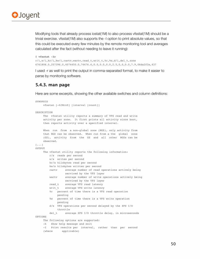
5.4.3. man page
Here are some excerpts, showing the other available switches and column definitions:
SYNOPSIS vfsstat [-hIMrzZ] [interval [count]]
DESCRIPTION The vfsstat utility reports a summary of VFS read and write activity per zone. It first prints all activity since boot, then reports activity over a specified interval.
When run from a non-global zone (NGZ), only activity from that NGZ can be observed. When run from a the global zone (GZ), activity from the GZ and all other NGZs can be observed.[...]OUTPUT The vfsstat utility reports the following information: r/s reads per second w/s writes per second kr/s kilobytes read per second kw/s kilobytes written per second ractv average number of read operations actively being serviced by the VFS layer wactv average number of write operations actively being serviced by the VFS layer read_t average VFS read latency writ_t average VFS write latency %r percent of time there is a VFS read operation pending %w percent of time there is a VFS write operation pending d/s VFS operations per second delayed by the ZFS I/O throttle del_t average ZFS I/O throttle delay, in microsecondsOPTIONS The following options are supported: -h Show help message and exit -I Print results per interval, rather than per second (where applicable)
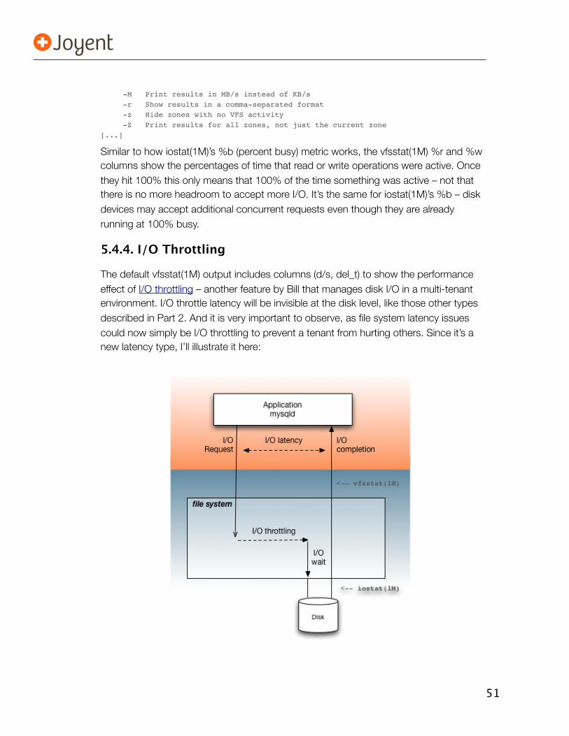
51
-M Print results in MB/s instead of KB/s -r Show results in a comma-separated format -z Hide zones with no VFS activity -Z Print results for all zones, not just the current zone[...]
Similar to how iostat(1M)’s %b (percent busy) metric works, the vfsstat(1M) %r and %w columns show the percentages of time that read or write operations were active. Once they hit 100% this only means that 100% of the time something was active – not that there is no more headroom to accept more I/O. It’s the same for iostat(1M)’s %b – disk devices may accept additional concurrent requests even though they are already running at 100% busy.
5.4.4. I/O Throttling
The default vfsstat(1M) output includes columns (d/s, del_t) to show the performance effect of I/O throttling – another feature by Bill that manages disk I/O in a multi-tenant environment. I/O throttle latency will be invisible at the disk level, like those other types described in Part 2. And it is very important to observe, as file system latency issues could now simply be I/O throttling to prevent a tenant from hurting others. Since it’s a new latency type, I’ll illustrate it here:
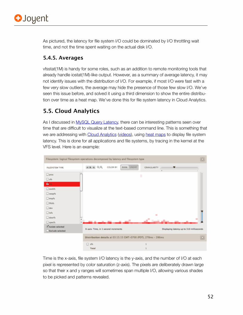
52
As pictured, the latency for file system I/O could be dominated by I/O throttling wait time, and not the time spent waiting on the actual disk I/O.
5.4.5. Averages
vfsstat(1M) is handy for some roles, such as an addition to remote monitoring tools that already handle iostat(1M)-like output. However, as a summary of average latency, it may not identify issues with the distribution of I/O. For example, if most I/O were fast with a few very slow outliers, the average may hide the presence of those few slow I/O. We’ve seen this issue before, and solved it using a third dimension to show the entire distribu-tion over time as a heat map. We’ve done this for file system latency in Cloud Analytics.
5.5. Cloud Analytics
As I discussed in MySQL Query Latency, there can be interesting patterns seen over time that are difficult to visualize at the text-based command line. This is something that we are addressing with Cloud Analytics (videos), using heat maps to display file system latency. This is done for all applications and file systems, by tracing in the kernel at the VFS level. Here is an example:
Time is the x-axis, file system I/O latency is the y-axis, and the number of I/O at each pixel is represented by color saturation (z-axis). The pixels are deliberately drawn large so that their x and y ranges will sometimes span multiple I/O, allowing various shades to be picked and patterns revealed.
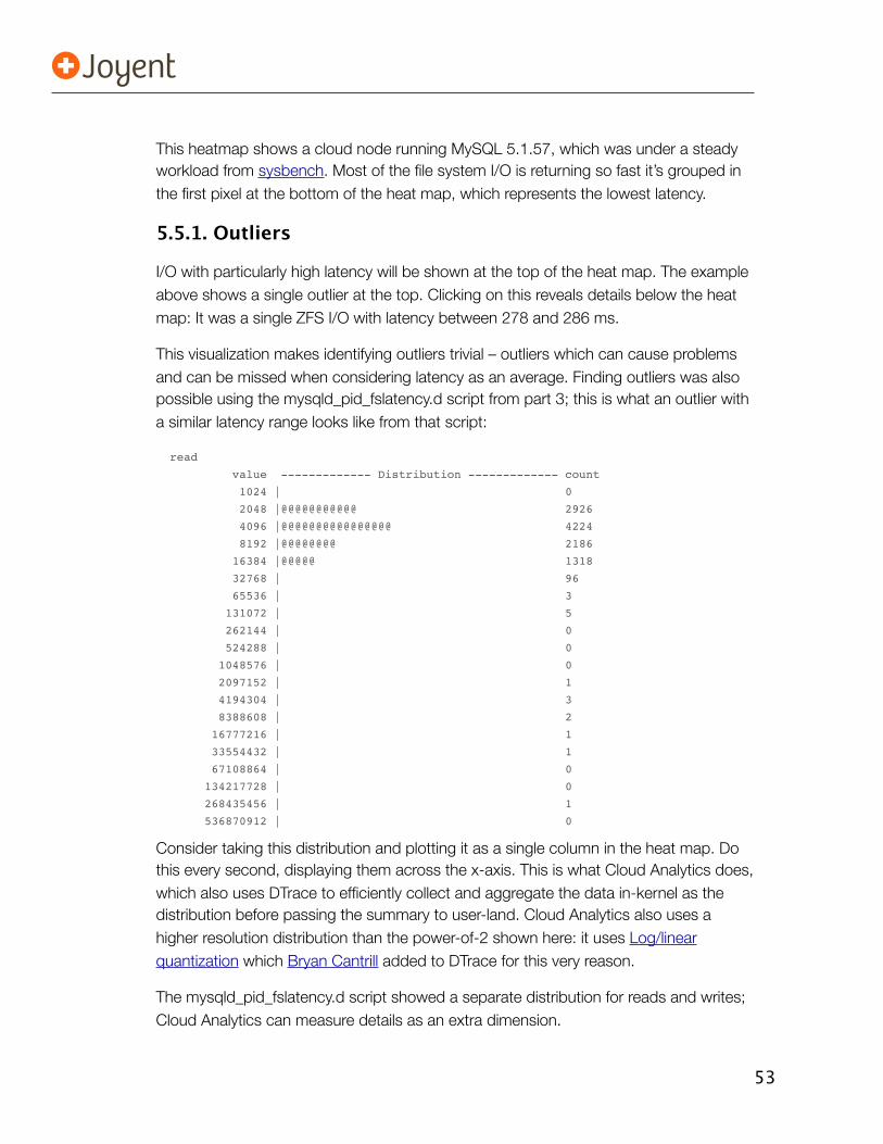
53
This heatmap shows a cloud node running MySQL 5.1.57, which was under a steady workload from sysbench. Most of the file system I/O is returning so fast it’s grouped in the first pixel at the bottom of the heat map, which represents the lowest latency.
5.5.1. Outliers
I/O with particularly high latency will be shown at the top of the heat map. The example above shows a single outlier at the top. Clicking on this reveals details below the heat map: It was a single ZFS I/O with latency between 278 and 286 ms.
This visualization makes identifying outliers trivial – outliers which can cause problems and can be missed when considering latency as an average. Finding outliers was also possible using the mysqld_pid_fslatency.d script from part 3; this is what an outlier with a similar latency range looks like from that script:
read
value ------------- Distribution ------------- count
1024 | 0
2048 |@@@@@@@@@@@ 2926
4096 |@@@@@@@@@@@@@@@@ 4224
8192 |@@@@@@@@ 2186
16384 |@@@@@ 1318
32768 | 96
65536 | 3
131072 | 5
262144 | 0
524288 | 0
1048576 | 0
2097152 | 1
4194304 | 3
8388608 | 2
16777216 | 1
33554432 | 1
67108864 | 0
134217728 | 0
268435456 | 1
536870912 | 0
Consider taking this distribution and plotting it as a single column in the heat map. Do this every second, displaying them across the x-axis. This is what Cloud Analytics does, which also uses DTrace to efficiently collect and aggregate the data in-kernel as the distribution before passing the summary to user-land. Cloud Analytics also uses a higher resolution distribution than the power-of-2 shown here: it uses Log/linear quantization which Bryan Cantrill added to DTrace for this very reason.
The mysqld_pid_fslatency.d script showed a separate distribution for reads and writes; Cloud Analytics can measure details as an extra dimension.
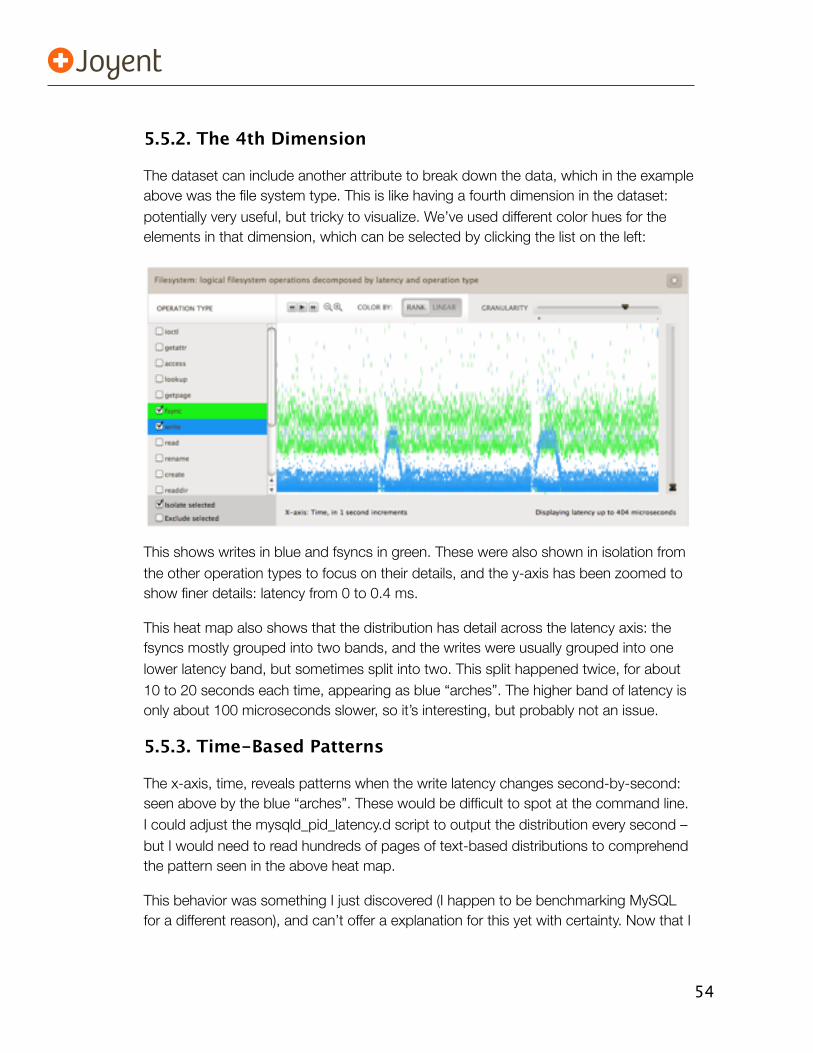
54
5.5.2. The 4th Dimension
The dataset can include another attribute to break down the data, which in the example above was the file system type. This is like having a fourth dimension in the dataset: potentially very useful, but tricky to visualize. We’ve used different color hues for the elements in that dimension, which can be selected by clicking the list on the left:
This shows writes in blue and fsyncs in green. These were also shown in isolation from the other operation types to focus on their details, and the y-axis has been zoomed to show finer details: latency from 0 to 0.4 ms.
This heat map also shows that the distribution has detail across the latency axis: the fsyncs mostly grouped into two bands, and the writes were usually grouped into one lower latency band, but sometimes split into two. This split happened twice, for about 10 to 20 seconds each time, appearing as blue “arches”. The higher band of latency is only about 100 microseconds slower, so it’s interesting, but probably not an issue.
5.5.3. Time-Based Patterns
The x-axis, time, reveals patterns when the write latency changes second-by-second: seen above by the blue “arches”. These would be difficult to spot at the command line. I could adjust the mysqld_pid_latency.d script to output the distribution every second – but I would need to read hundreds of pages of text-based distributions to comprehend the pattern seen in the above heat map.
This behavior was something I just discovered (I happen to be benchmarking MySQL for a different reason), and can’t offer a explanation for this yet with certainty. Now that I
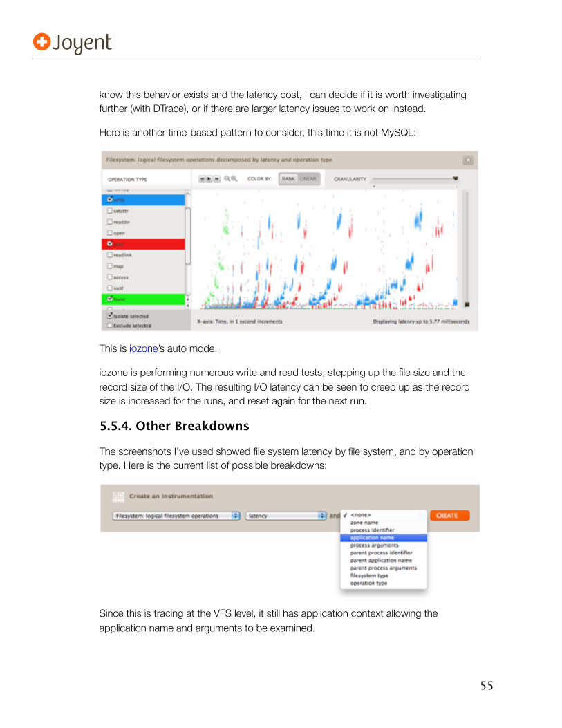
55
know this behavior exists and the latency cost, I can decide if it is worth investigating further (with DTrace), or if there are larger latency issues to work on instead.
Here is another time-based pattern to consider, this time it is not MySQL:
This is iozone’s auto mode.
iozone is performing numerous write and read tests, stepping up the file size and the record size of the I/O. The resulting I/O latency can be seen to creep up as the record size is increased for the runs, and reset again for the next run.
5.5.4. Other Breakdowns
The screenshots I’ve used showed file system latency by file system, and by operation type. Here is the current list of possible breakdowns:
Since this is tracing at the VFS level, it still has application context allowing the application name and arguments to be examined.
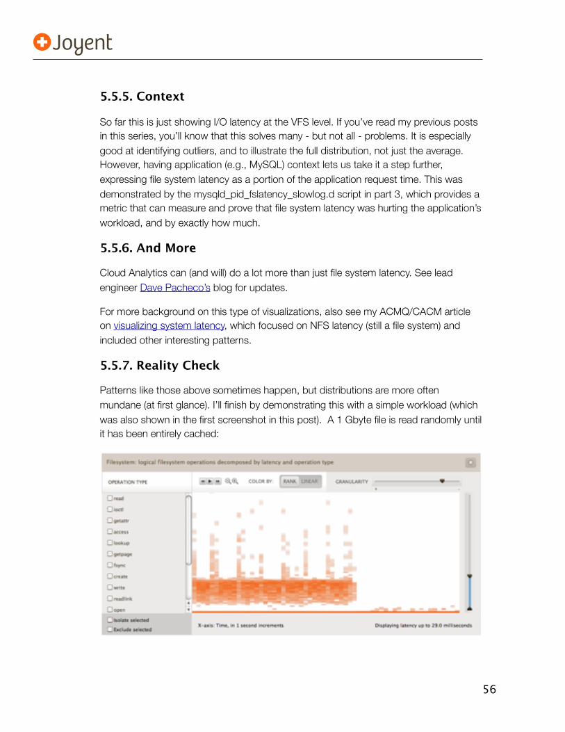
56
5.5.5. Context
So far this is just showing I/O latency at the VFS level. If you’ve read my previous posts in this series, you’ll know that this solves many - but not all - problems. It is especially good at identifying outliers, and to illustrate the full distribution, not just the average. However, having application (e.g., MySQL) context lets us take it a step further, expressing file system latency as a portion of the application request time. This was demonstrated by the mysqld_pid_fslatency_slowlog.d script in part 3, which provides a metric that can measure and prove that file system latency was hurting the application’s workload, and by exactly how much.
5.5.6. And More
Cloud Analytics can (and will) do a lot more than just file system latency. See lead engineer Dave Pacheco’s blog for updates.
For more background on this type of visualizations, also see my ACMQ/CACM article on visualizing system latency, which focused on NFS latency (still a file system) and included other interesting patterns.
5.5.7. Reality Check
Patterns like those above sometimes happen, but distributions are more often mundane (at first glance). I’ll finish by demonstrating this with a simple workload (which was also shown in the first screenshot in this post). A 1 Gbyte file is read randomly until it has been entirely cached:
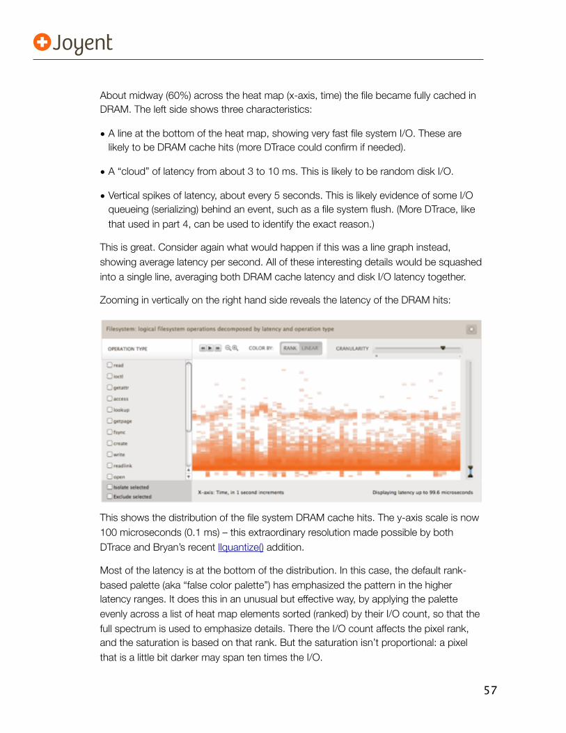
57
About midway (60%) across the heat map (x-axis, time) the file became fully cached in DRAM. The left side shows three characteristics:
• A line at the bottom of the heat map, showing very fast file system I/O. These are likely to be DRAM cache hits (more DTrace could confirm if needed).
• A “cloud” of latency from about 3 to 10 ms. This is likely to be random disk I/O.
• Vertical spikes of latency, about every 5 seconds. This is likely evidence of some I/O queueing (serializing) behind an event, such as a file system flush. (More DTrace, like that used in part 4, can be used to identify the exact reason.)
This is great. Consider again what would happen if this was a line graph instead, showing average latency per second. All of these interesting details would be squashed into a single line, averaging both DRAM cache latency and disk I/O latency together.
Zooming in vertically on the right hand side reveals the latency of the DRAM hits:
This shows the distribution of the file system DRAM cache hits. The y-axis scale is now 100 microseconds (0.1 ms) – this extraordinary resolution made possible by both DTrace and Bryan’s recent llquantize() addition.
Most of the latency is at the bottom of the distribution. In this case, the default rank-based palette (aka “false color palette”) has emphasized the pattern in the higher latency ranges. It does this in an unusual but effective way, by applying the palette evenly across a list of heat map elements sorted (ranked) by their I/O count, so that the full spectrum is used to emphasize details. There the I/O count affects the pixel rank, and the saturation is based on that rank. But the saturation isn’t proportional: a pixel that is a little bit darker may span ten times the I/O.
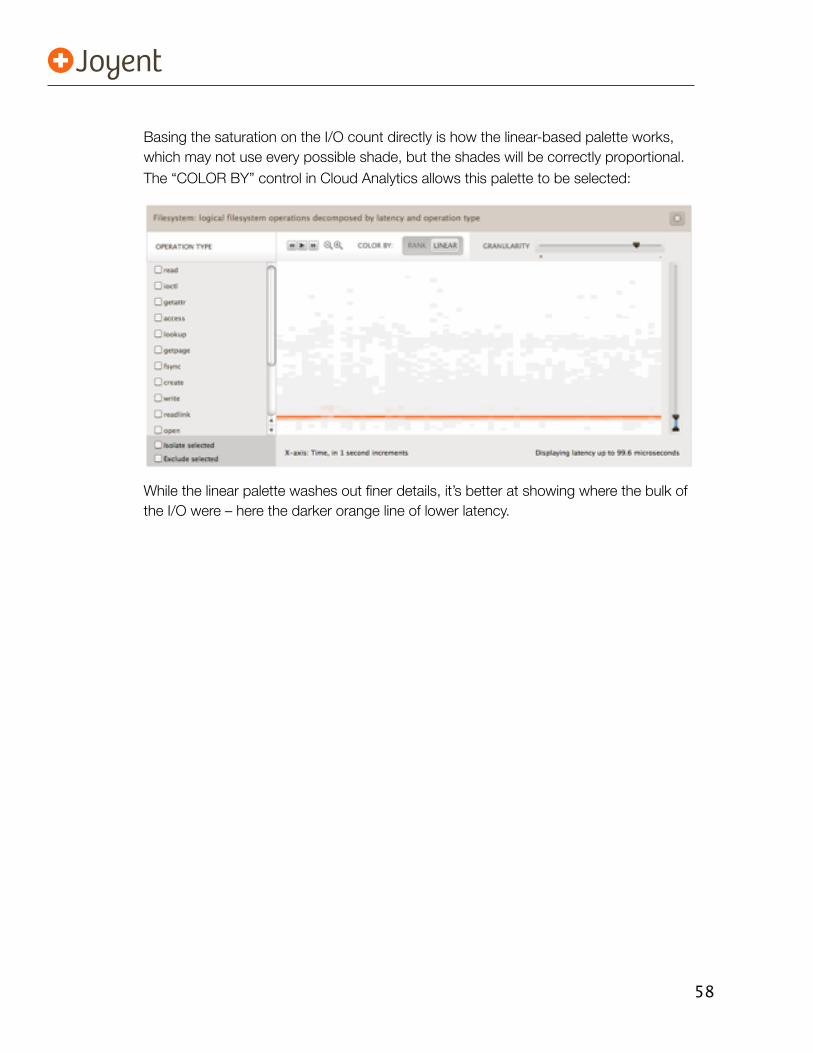
58
Basing the saturation on the I/O count directly is how the linear-based palette works, which may not use every possible shade, but the shades will be correctly proportional. The “COLOR BY” control in Cloud Analytics allows this palette to be selected:
While the linear palette washes out finer details, it’s better at showing where the bulk of the I/O were – here the darker orange line of lower latency.
59
6. ConclusionWith increased functionality and caching of file systems rendering disk-level metrics confusing and incomplete, file system latency has become an essential metric for understanding application performance. In this paper, various DTrace-based tools were introduced to measure file system latency, with the most effective expressing it as a synchronous component of the application workload - demonstrated here by the sum of file system latency during a MySQL query. I’ve been using these tools for several months to solve real world performance issues in a cloud computing environment.
Various ways to present file system latency were also shown. These included a new command line tool, vfsstat(1M), which provides numerical summaries of VFS level latency at regular intervals, in a format that can be consumed by both system administrators and remote monitoring tools. Joyent’s Cloud Analytics showed how heat maps could present file system latency in much greater detail, showing the entire distribution and allowing latency outliers to be easily identified. And DTrace at the command line showed how latency could be presented event-by-event, and at any layer of the operating system stack from the application interface to the kernel device drivers, to pinpoint the origin of any slowdowns.
60
References
• Solaris Internals 2nd Ed. – Jim Mauro, Richard McDougall (Prentice Hall, 2006)
• Solaris Performance and Tools – Richard McDougall, Jim Mauro, Brendan Gregg
(Prentice Hall, 2006)
• DTrace – Brendan Gregg, Jim Mauro (Prentice Hall, 2011)
• http://learningsolaris.com/docs/dtrace_usenix.pdf – Original DTrace whitepaper
• http://www.brendangregg.com/dtrace.html#DTraceToolkit – DTraceToolkit
• http://dtrace.org – DTrace blogs
• http://dtrace.org/blogs/brendan – Brendan Gregg’s blog
• http://dtrace.org/blogs/brendan/2011/06/23/mysql-performance-schema-and-dtrace
– Tracing the MySQL performance_schema using DTrace
• http://dtrace.org/blogs/brendan/2011/03/14/mysql-query-latency-with-the-dtrace-
pid-provider – MySQL query latency using DTrace
• http://dtrace.org/blogs/brendan/2011/02/19/dtrace-pid-provider-links – DTrace pid
provider articles
• http://dtrace.org/blogs/wdp/2011/03/our-zfs-io-throttle – ZFS I/O throttling
• http://dtrace.org/blogs/bmc/2011/02/08/llquantize – DTrace log/linear quantization
• http://www.markleith.co.uk – Mark Leith’s blog
• http://www.latencytop.org – LatencyTOP homepage
• http://sourceware.org/systemtap – SystemTap homepage
• http://smartos.org – SmartOS homepage
61
• http://www.illumos.org – Illumos homepage
• http://www.joyent.com/products/smartdatacenter – Joyent SmartDataCenter
• http://sysbench.sourceforge.net – SysBench performance benchmark
• http://www.iozone.org – IOzone performance benchmark
• http://queue.acm.org/detail.cfm?id=1809426 – Visualizing System Latency
• http://dtrace.org/blogs/dap/2011/03/01/welcome-to-cloud-analytics – Cloud
Analytics announcement
• http://dtrace.org/blogs/brendan/2011/01/24/cloud-analytics-first-video – Cloud
Analytics video