Examining ASTER Imagery with the MapPlace Image Analysis Toolbox

A Tutorial Manual

By W.E. Kilby and C.E. Kilby Cal Data Ltd

Geoscience BC Report 2006-3 British Columbia Contribution #GBC 015 Ministry of Energy, Mines and Petroleum Resources GeoFile 2006-8

ii

iii

TABLE OF CONTENTS

INTRODUCTION ........................................................................................................... 1

IMAGE ANALYSIS TOOLBOX ........................................................................................ 1 Purpose ......................................................................................................................... 1 Imagery......................................................................................................................... 2 Image Pre-processing .................................................................................................. 3

IMAGE ANALYSIS TOOLBOX – INDEX PAGE ........................................................... 4 Operation...................................................................................................................... 4 To View ASTER images.............................................................................................. 6 To View partially covered images .............................................................................. 7 An alternative image selection method ...................................................................... 8 Proceeding to Analysis ................................................................................................ 8 One-Band Analysis ........................................................................................ 9 Applying mask.................................................................................... 12 Applying MASKER ........................................................................... 12 Three-Band Analysis ................................................................................... 13 To use MASKER................................................................................ 15 Two-Band Analysis...................................................................................... 15 To use MASKER................................................................................ 17 FCC – False Colour Composite Analysis .................................................. 17 To use MASKER................................................................................ 18 NDVI Vegetation Analysis .......................................................................... 19 To use MASKER................................................................................ 21 Tasseled Cap Transformation .................................................................... 21 Spectral Angle Mapper ............................................................................... 21 To use MASKER................................................................................ 22 Prepared Images ........................................................................................................ 23 Anaglyph Map ............................................................................................. 23 Virtual Reality ............................................................................................. 25 Google Earth ................................................................................................ 27 Download Page............................................................................................. 31 Original ASTER Data........................................................................ 32 ASTER DEM ...................................................................................... 32 Virtual Reality File............................................................................. 34 Stereo Pair Images ............................................................................. 34 Anaglyph Image ................................................................................. 35 Alteration-Mineral Images................................................................ 35

ACKNOWLEDGEMENTS................................................................................................ 37

REFERENCES.................................................................................................................... 37

iv

1

Examining ASTER Imagery with the MapPlace Image Analysis Toolbox

A Tutorial Manual

INTRODUCTION Remote sensing images have been continually added to the MapPlace since 2003. The image

analysis toolbox was created to utilize this data. Making use of such image data is new for many clients of the website. This manual is provided as an introduction to ASTER imagery and to assist users in navigating the toolbox. Portions of this manual are derived from three B.C. Geological Survey papers in Fieldwork: Kilby et al. (2004), Kilby (2005) and Kilby and Kilby (2006), and many other sources noted in the text or under References at the end of the manual.

Advanced Spaceborne Thermal Emission and Reflection Radiometer (ASTER) is an imaging instrument flying on the Terra satellite, launched in late 1999. ASTER is a cooperative project between NASA, Japan’s Ministry of Economy, Trade and Industry and Japan’s Earth Remote Sensing Data Analysis Center. The instrument has 3 subsystems that capture readings from different portions of the electromagnetic spectrum at different resolutions. The three subsystems are referred to as VNIR (Visible and Near Infrared), SWIR (Shortwave Infrared) and TIR (Thermal Infrared). Reflectance values in the SWIR range are particularly useful in differentiating rock and soil mineralogy related to alteration zones.

An ASTER image contains 14 bands of information, 4 bands in the VNIR with 15 metre resolution, 6 bands in the SWIR with 30 metre resolution and 5 bands in the TIR with 90 metre resolution. Two of the VNIR bands sample the same wavelength range but one is back-looking providing the ability to generate a stereo view of the scene. A single ASTER scene covers an area of about 60 by 60 kilometres. The ASTER web site http://asterweb.jpl.nasa.gov is an excellent source of information on the instrument, its mission, available imagery, usage examples and analysis tools.

The “Image Analysis Toolbox” project developed and implemented an image analysis capability for the MapPlace and was delivered by Cal Data Ltd. The Toolbox is a framework in which a variety of multi and hyperspectral imagery can be added and processed online by end users. The results of the analysis are georeferenced and can be completely integrated with the information already contained in the MapPlace.

IMAGE ANALYSIS TOOLBOX

Purpose The Image Analysis Toolbox (IAT) was developed to be a system that could hold multispectral

and hyperspectral imagery, analyze the imagery and display it through the MapPlace. A suite of analysis tools have been provided. The IAT was added to the Exploration Assistant page of the

2

MapPlace. The appearance and operation of the IAT was designed to maintain the general look and feel of the Exploration Assistant. The purpose of the Toolbox is to provide the ability for MapPlace users to experiment with a variety of imagery and analysis procedures in their search for exploration targets.

Imagery In April 2006 there were 68 Landsat 7 and 139 ASTER multispectral images, and one each of

HYPERION and AVIRIS hyperspectral images included in the IAT. In this manual we focus on analytical processes available with the IAT and their use on ASTER imagery.

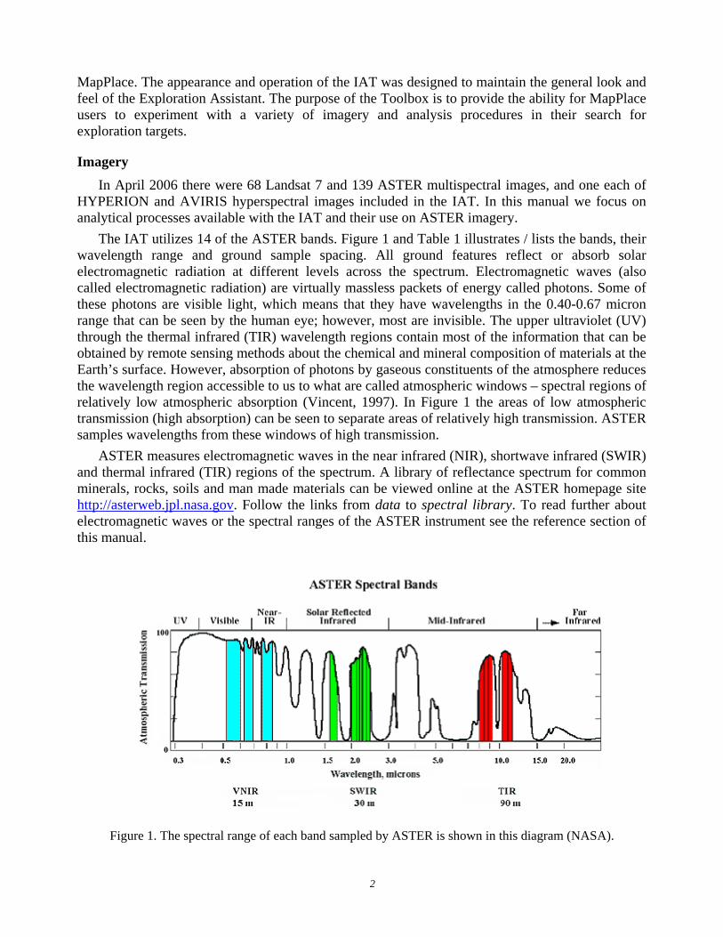
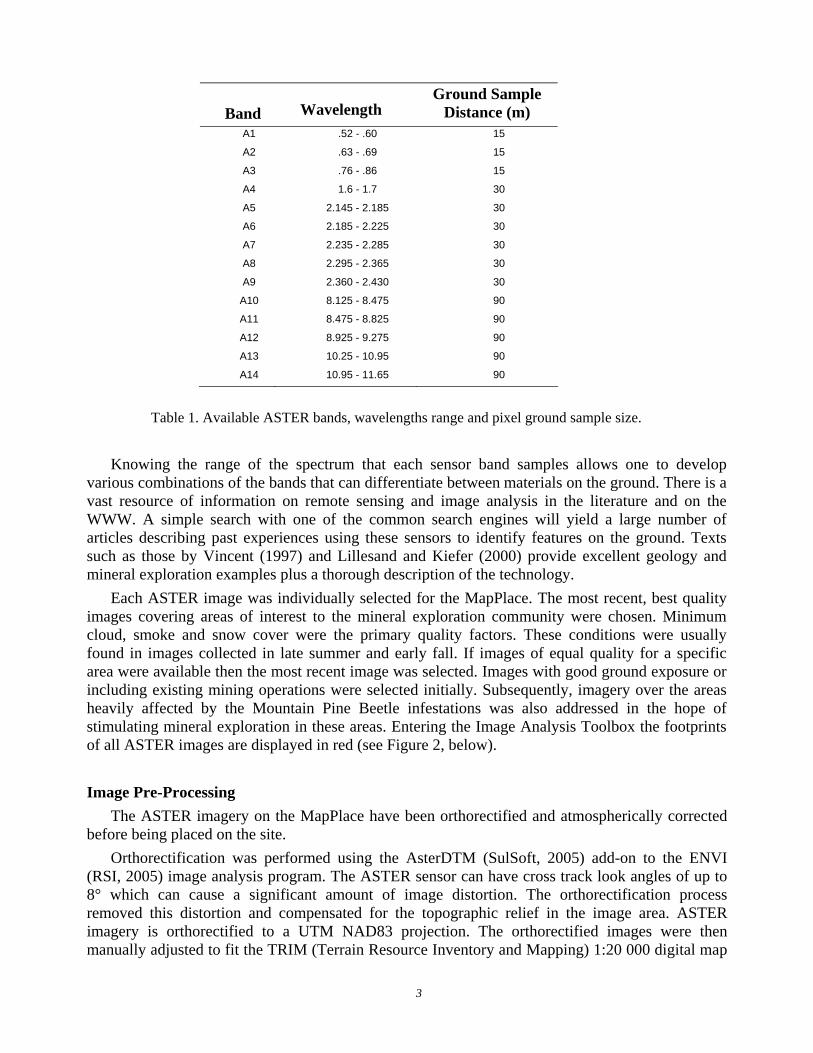
The IAT utilizes 14 of the ASTER bands. Figure 1 and Table 1 illustrates / lists the bands, their wavelength range and ground sample spacing. All ground features reflect or absorb solar electromagnetic radiation at different levels across the spectrum. Electromagnetic waves (also called electromagnetic radiation) are virtually massless packets of energy called photons. Some of these photons are visible light, which means that they have wavelengths in the 0.40-0.67 micron range that can be seen by the human eye; however, most are invisible. The upper ultraviolet (UV) through the thermal infrared (TIR) wavelength regions contain most of the information that can be obtained by remote sensing methods about the chemical and mineral composition of materials at the Earth’s surface. However, absorption of photons by gaseous constituents of the atmosphere reduces the wavelength region accessible to us to what are called atmospheric windows – spectral regions of relatively low atmospheric absorption (Vincent, 1997). In Figure 1 the areas of low atmospheric transmission (high absorption) can be seen to separate areas of relatively high transmission. ASTER samples wavelengths from these windows of high transmission.

ASTER measures electromagnetic waves in the near infrared (NIR), shortwave infrared (SWIR) and thermal infrared (TIR) regions of the spectrum. A library of reflectance spectrum for common minerals, rocks, soils and man made materials can be viewed online at the ASTER homepage site http://asterweb.jpl.nasa.gov. Follow the links from data to spectral library. To read further about electromagnetic waves or the spectral ranges of the ASTER instrument see the reference section of this manual.

Figure 1. The spectral range of each band sampled by ASTER is shown in this diagram (NASA).

3

Band Wavelength Ground Sample

Distance (m) A1 .52 - .60 15

A2 .63 - .69 15

A3 .76 - .86 15

A4 1.6 - 1.7 30

A5 2.145 - 2.185 30

A6 2.185 - 2.225 30

A7 2.235 - 2.285 30

A8 2.295 - 2.365 30

A9 2.360 - 2.430 30

A10 8.125 - 8.475 90

A11 8.475 - 8.825 90

A12 8.925 - 9.275 90

A13 10.25 - 10.95 90

A14 10.95 - 11.65 90

Table 1. Available ASTER bands, wavelengths range and pixel ground sample size. Knowing the range of the spectrum that each sensor band samples allows one to develop

various combinations of the bands that can differentiate between materials on the ground. There is a vast resource of information on remote sensing and image analysis in the literature and on the WWW. A simple search with one of the common search engines will yield a large number of articles describing past experiences using these sensors to identify features on the ground. Texts such as those by Vincent (1997) and Lillesand and Kiefer (2000) provide excellent geology and mineral exploration examples plus a thorough description of the technology.

Each ASTER image was individually selected for the MapPlace. The most recent, best quality images covering areas of interest to the mineral exploration community were chosen. Minimum cloud, smoke and snow cover were the primary quality factors. These conditions were usually found in images collected in late summer and early fall. If images of equal quality for a specific area were available then the most recent image was selected. Images with good ground exposure or including existing mining operations were selected initially. Subsequently, imagery over the areas heavily affected by the Mountain Pine Beetle infestations was also addressed in the hope of stimulating mineral exploration in these areas. Entering the Image Analysis Toolbox the footprints of all ASTER images are displayed in red (see Figure 2, below).

Image Pre-Processing

The ASTER imagery on the MapPlace have been orthorectified and atmospherically corrected before being placed on the site.

Orthorectification was performed using the AsterDTM (SulSoft, 2005) add-on to the ENVI (RSI, 2005) image analysis program. The ASTER sensor can have cross track look angles of up to 8° which can cause a significant amount of image distortion. The orthorectification process removed this distortion and compensated for the topographic relief in the image area. ASTER imagery is orthorectified to a UTM NAD83 projection. The orthorectified images were then manually adjusted to fit the TRIM (Terrain Resource Inventory and Mapping) 1:20 000 digital map

4

data displayed on the MapPlace. This manual adjustment was necessary to compensate for a.) some ASTER positioning errors “Over the last 5 years, we have discovered several small errors that can affect the accuracy of these coordinates: …” (NASA Jet Propulsion Laboratory, 2005) and b.) errors in TRIM data. For the purposes of this project registration to the TRIM data provided the most appropriate adjustment.

Atmospheric corrections were performed on the VNIR (Visible and Near Infrared) and SWIR (Short Wave Infrared) bands in all the images using the ACORN5 (Atmospheric CORrection Now) program (ImSpec, 2004). This program performs a radiance to relative reflectance correction of the image values by removing the effect of water vapour and other gasses in the atmosphere using the MOTRAN4 technology. ACORN5 also corrects for atmospheric scattering as well as the shape of the solar irradiance curve that is variable by wavelength depending on solar incidence angle. ASTER imagery does not contain enough information to calculate the amount of water vapour found within an image so a standard value of 15 millimetres of atmospheric water was used for all images. Atmospheric water content obviously varies between ASTER scenes and within the scenes but the value of 15 millimetres was selected as representative after a review of the MODIS Atmosphere Profile Product record (NASA MODIS Atmosphere, 2005). Atmospheric correction enhances the digital information available to the IAT from simple DN (uncalibrated instrument readings) values to relative reflectance values that more accurately portray the true reflectance spectra of a ground sample area. The relative reflectance values allow comparison of the image pixel spectra with natural and man made materials in existing reflectance spectral libraries such as the ASTER Spectral Library available on-line (NASA, 2000).

IMAGE ANALYSIS TOOLBOX – INDEX PAGE

Operation This section describes the operation of the system from the client’s perspective. Enter the

Exploration Assistant. The right panel lists optional tools for exploration analysis. Choose the Image Analysis Toolbox button. This will take the user to the Image Analysis Toolbox index page.

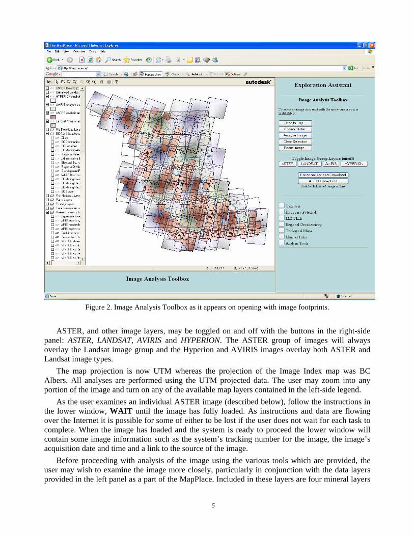
A new right panel labelled “Image Analysis Toolbox” will appear and several new layers will be added to the map (Figure 2). Colored squares, or “footprints” of all images will be visible (Landsat, ASTER, AVIRIS and Hyperion) at a scale larger than 1:6 000 000. The images are presented as a stack of blue, red, dark red and green coloured squares, often overlapping each other. The footprints from Hyperion and AVIRIS are almost invisible at this scale. At any point the user may return to one of the other Exploration Assistant tools by using the buttons in the lower right panel.

5

Figure 2. Image Analysis Toolbox as it appears on opening with image footprints.

ASTER, and other image layers, may be toggled on and off with the buttons in the right-side

panel: ASTER, LANDSAT, AVIRIS and HYPERION. The ASTER group of images will always overlay the Landsat image group and the Hyperion and AVIRIS images overlay both ASTER and Landsat image types.

The map projection is now UTM whereas the projection of the Image Index map was BC Albers. All analyses are performed using the UTM projected data. The user may zoom into any portion of the image and turn on any of the available map layers contained in the left-side legend.

As the user examines an individual ASTER image (described below), follow the instructions in the lower window, WAIT until the image has fully loaded. As instructions and data are flowing over the Internet it is possible for some of either to be lost if the user does not wait for each task to complete. When the image has loaded and the system is ready to proceed the lower window will contain some image information such as the system’s tracking number for the image, the image’s acquisition date and time and a link to the source of the image.

Before proceeding with analysis of the image using the various tools which are provided, the user may wish to examine the image more closely, particularly in conjunction with the data layers provided in the left panel as a part of the MapPlace. Included in these layers are four mineral layers

6

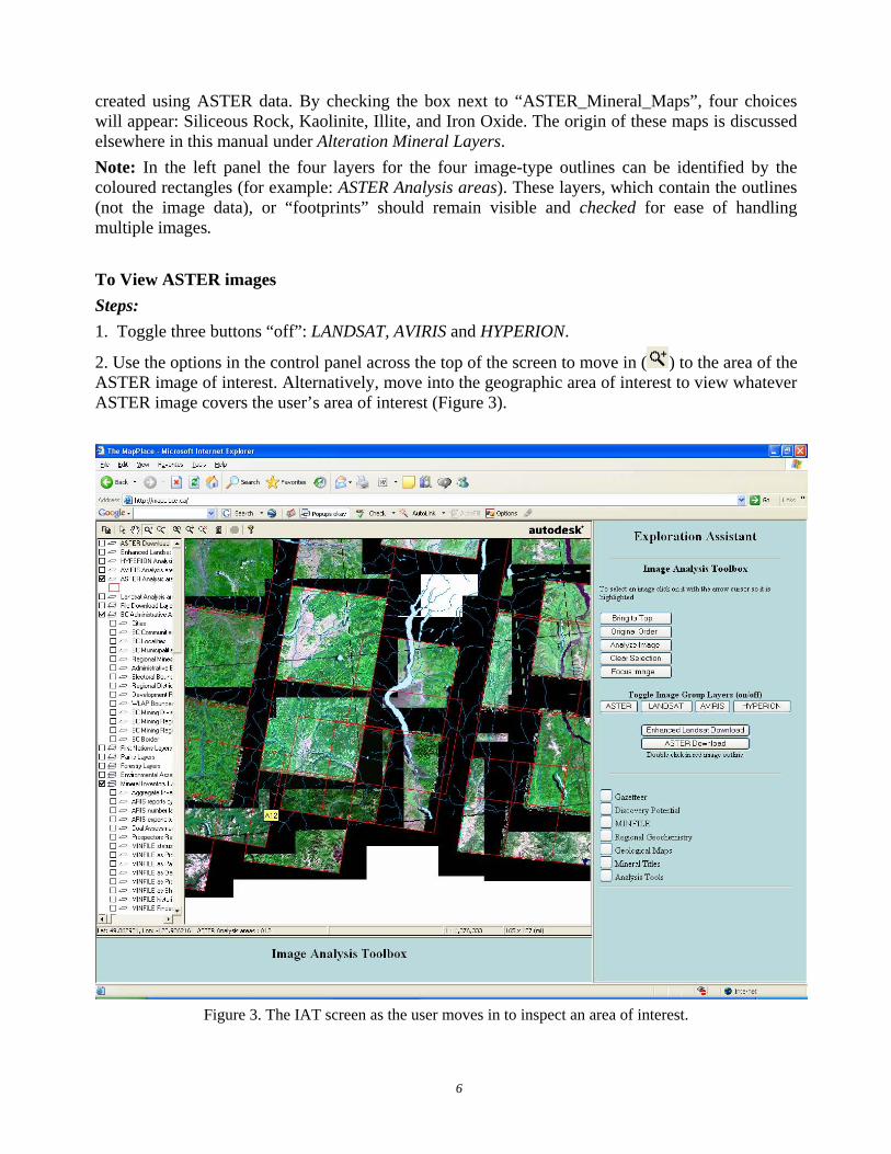
created using ASTER data. By checking the box next to “ASTER_Mineral_Maps”, four choices will appear: Siliceous Rock, Kaolinite, Illite, and Iron Oxide. The origin of these maps is discussed elsewhere in this manual under Alteration Mineral Layers. Note: In the left panel the four layers for the four image-type outlines can be identified by the coloured rectangles (for example: ASTER Analysis areas). These layers, which contain the outlines (not the image data), or “footprints” should remain visible and checked for ease of handling multiple images.

To View ASTER images Steps: 1. Toggle three buttons “off”: LANDSAT, AVIRIS and HYPERION.

2. Use the options in the control panel across the top of the screen to move in ( ) to the area of the ASTER image of interest. Alternatively, move into the geographic area of interest to view whatever ASTER image covers the user’s area of interest (Figure 3).

Figure 3. The IAT screen as the user moves in to inspect an area of interest.

7

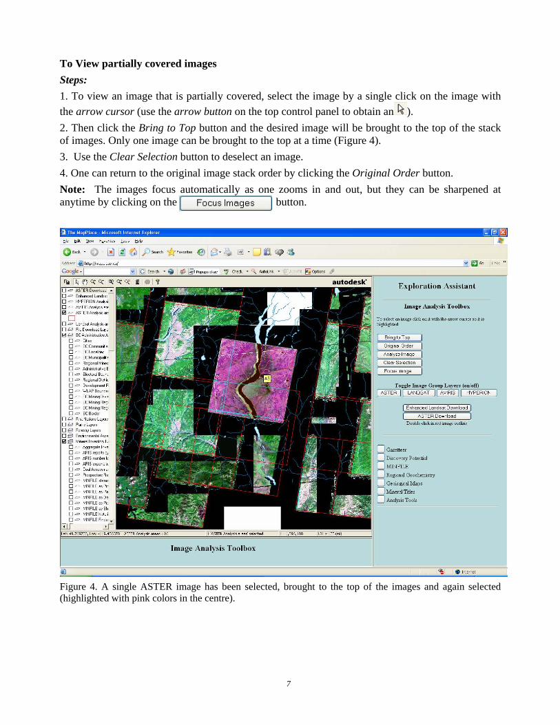
To View partially covered images Steps: 1. To view an image that is partially covered, select the image by a single click on the image with the arrow cursor (use the arrow button on the top control panel to obtain an ). 2. Then click the Bring to Top button and the desired image will be brought to the top of the stack of images. Only one image can be brought to the top at a time (Figure 4). 3. Use the Clear Selection button to deselect an image. 4. One can return to the original image stack order by clicking the Original Order button. Note: The images focus automatically as one zooms in and out, but they can be sharpened at anytime by clicking on the button.

Figure 4. A single ASTER image has been selected, brought to the top of the images and again selected (highlighted with pink colors in the centre).

8

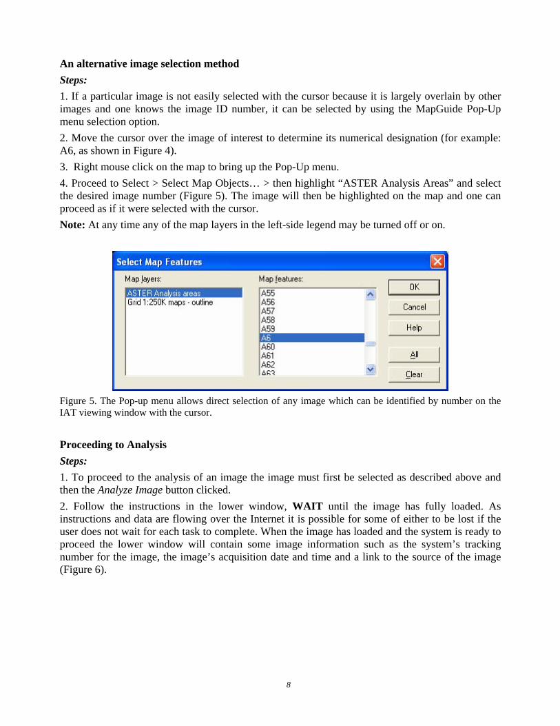
An alternative image selection method Steps: 1. If a particular image is not easily selected with the cursor because it is largely overlain by other images and one knows the image ID number, it can be selected by using the MapGuide Pop-Up menu selection option. 2. Move the cursor over the image of interest to determine its numerical designation (for example: A6, as shown in Figure 4). 3. Right mouse click on the map to bring up the Pop-Up menu. 4. Proceed to Select > Select Map Objects… > then highlight “ASTER Analysis Areas” and select the desired image number (Figure 5). The image will then be highlighted on the map and one can proceed as if it were selected with the cursor. Note: At any time any of the map layers in the left-side legend may be turned off or on.

Figure 5. The Pop-up menu allows direct selection of any image which can be identified by number on the IAT viewing window with the cursor.

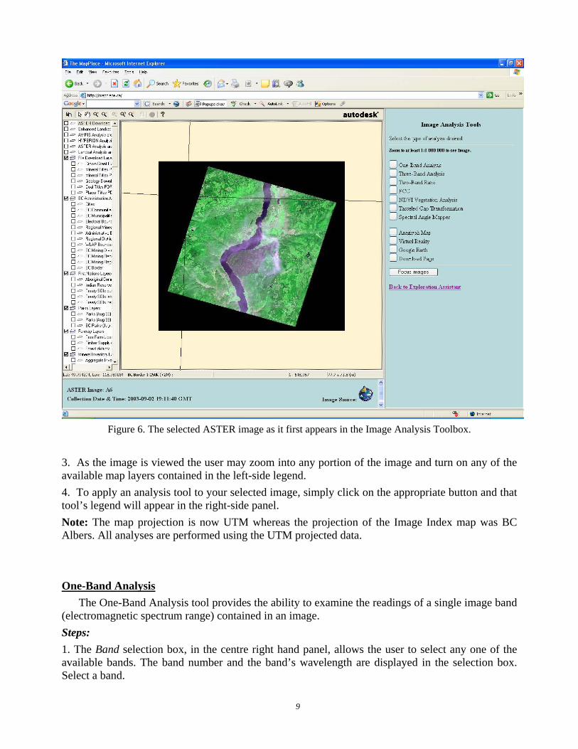
Proceeding to Analysis Steps: 1. To proceed to the analysis of an image the image must first be selected as described above and then the Analyze Image button clicked. 2. Follow the instructions in the lower window, WAIT until the image has fully loaded. As instructions and data are flowing over the Internet it is possible for some of either to be lost if the user does not wait for each task to complete. When the image has loaded and the system is ready to proceed the lower window will contain some image information such as the system’s tracking number for the image, the image’s acquisition date and time and a link to the source of the image (Figure 6).

9

Figure 6. The selected ASTER image as it first appears in the Image Analysis Toolbox.

3. As the image is viewed the user may zoom into any portion of the image and turn on any of the available map layers contained in the left-side legend. 4. To apply an analysis tool to your selected image, simply click on the appropriate button and that tool’s legend will appear in the right-side panel. Note: The map projection is now UTM whereas the projection of the Image Index map was BC Albers. All analyses are performed using the UTM projected data. One-Band Analysis

The One-Band Analysis tool provides the ability to examine the readings of a single image band (electromagnetic spectrum range) contained in an image. Steps: 1. The Band selection box, in the centre right hand panel, allows the user to select any one of the available bands. The band number and the band’s wavelength are displayed in the selection box. Select a band.

10

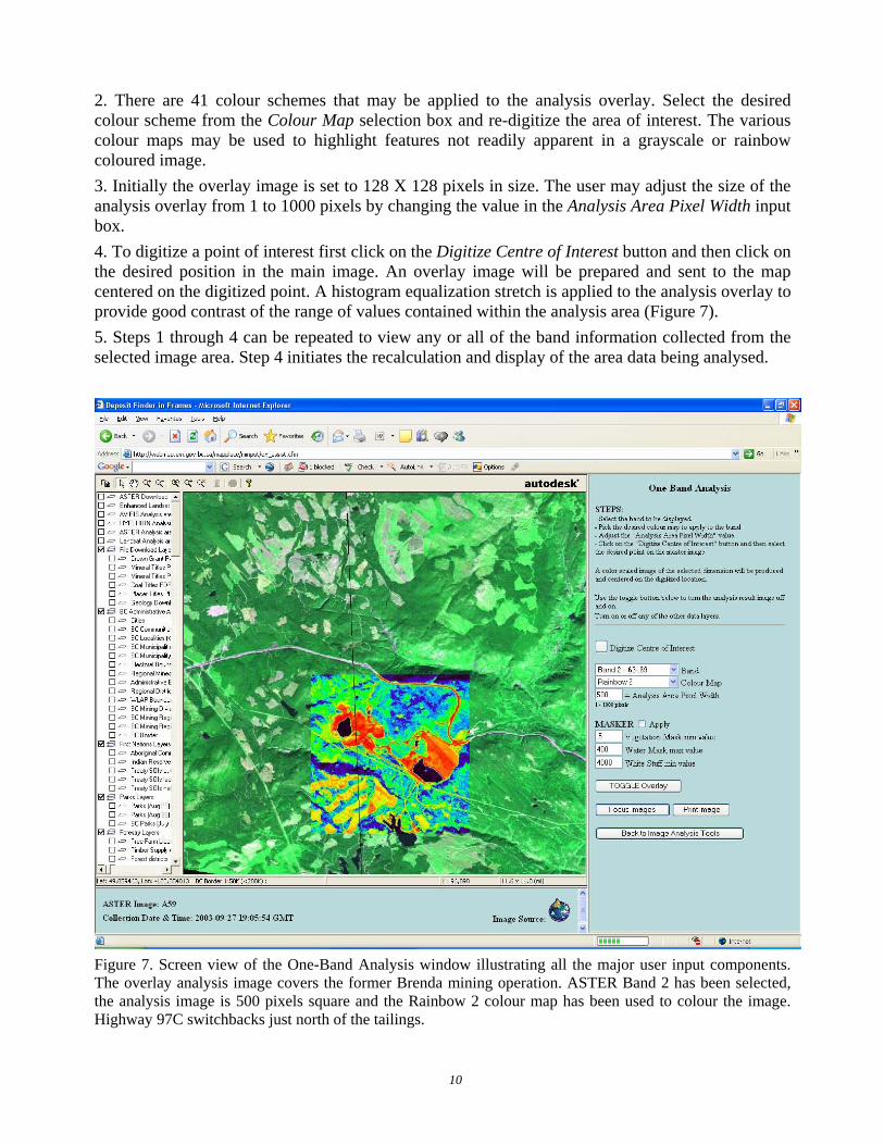
2. There are 41 colour schemes that may be applied to the analysis overlay. Select the desired colour scheme from the Colour Map selection box and re-digitize the area of interest. The various colour maps may be used to highlight features not readily apparent in a grayscale or rainbow coloured image. 3. Initially the overlay image is set to 128 X 128 pixels in size. The user may adjust the size of the analysis overlay from 1 to 1000 pixels by changing the value in the Analysis Area Pixel Width input box. 4. To digitize a point of interest first click on the Digitize Centre of Interest button and then click on the desired position in the main image. An overlay image will be prepared and sent to the map centered on the digitized point. A histogram equalization stretch is applied to the analysis overlay to provide good contrast of the range of values contained within the analysis area (Figure 7). 5. Steps 1 through 4 can be repeated to view any or all of the band information collected from the selected image area. Step 4 initiates the recalculation and display of the area data being analysed.

Figure 7. Screen view of the One-Band Analysis window illustrating all the major user input components. The overlay analysis image covers the former Brenda mining operation. ASTER Band 2 has been selected, the analysis image is 500 pixels square and the Rainbow 2 colour map has been used to colour the image. Highway 97C switchbacks just north of the tailings.

11

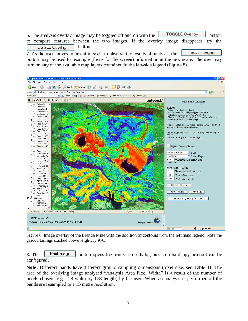
6. The analysis overlay image may be toggled off and on with the button to compare features between the two images. If the overlay image disappears, try the button. button. 7. As the user moves in or out in scale to observe the results of analysis, the ( ) button may be used to resample (focus for the screen) information at the new scale. The user may turn on any of the available map layers contained in the left-side legend (Figure 8).

Figure 8. Image overlay of the Brenda Mine with the addition of contours from the left hand legend. Note the graded tailings stacked above Highway 97C. 8. The button opens the prints setup dialog box so a hardcopy printout can be configured. Note: Different bands have different ground sampling dimensions (pixel size, see Table 1). The area of the overlying image analysed “Analysis Area Pixel Width” is a result of the number of pixels chosen (e.g. 128 width by 128 length) by the user. When an analysis is performed all the bands are resampled to a 15 metre resolution.

12

Note: Use the button to return to the Image Analysis Tools page.

Applying mask

A major problem with analyzing a large area such as a whole ASTER image is that many very different types of surfaces are included in the analysis, often making subtle differences in the spectra of a target area difficult to identify. A traditional method of overcoming this problem is to apply a mask that removes all but the area of interest from the calculation. Such a mask may be calculated for each image or portion of an image and used to constrain the area of the image being analyzed.

Applying MASKER

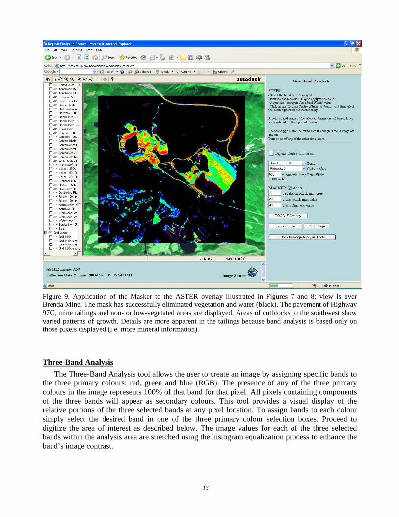
Application of the MASKER can blank out all areas covered by vegetation, clouds, water, snow and ice; hopefully, leaving only those pixels that sampled good ground exposures. A simple check box in the individual tool panel of the IAT allows the user to make use of the mask when desired. Steps: 1. To utilize the masking technique the MASKER…..Apply box, in the right-hand panel should be checked. 2. Then the Digitize Centre of Interest button should be used and a point selected on the image (Figure 9). Follow the instructions in the lower window, WAIT until the image has fully loaded. The user must adjust the mask for their own use. Three values may be adjusted to create a good mask for a specific area of interest on an ASTER image; values in areas of vegetation, water and areas of white-out within an image. Default values are provided initially for these three options. 3. For example the Water Mask max value may be adjusted. Find a lake in the image close to an area of interest and use the Digitize Centre of Interest button and select a point in the lake, including some shore. The goal is to create a black mask over the lake, or portion of the lake in the field of view. If some areas of color still occur over the lake after applying the default value, adjust this value in the Water Mask max value box and repeat steps 1 to 3. This is an iterative process, but will allow the user to fine tune the area to be masked. 4. In a similar way the Vegetation Mask min value could be adjusted to best cover the vegetation in the user’s field of view. 5. The White Stuff min value is to be used where snow, ice or excessive clouds are found adjacent to an area of interest. Eliminating the white pixels from the calculations will greatly improve the representation of the selected band analysis of an area on the ASTER image. Note: The masking algorithms which produce the black mask remove the vast majority of the pixels measuring non-rock surfaces but there are always some pixels which include mixtures of rock and non-rock materials. The user should use caution when interpreting analysis results using these masks to ascertain that a pixel of interest did in fact sample a rock surface

13

Figure 9. Application of the Masker to the ASTER overlay illustrated in Figures 7 and 8; view is over Brenda Mine. The mask has successfully eliminated vegetation and water (black). The pavement of Highway 97C, mine tailings and non- or low-vegetated areas are displayed. Areas of cutblocks to the southwest show varied patterns of growth. Details are more apparent in the tailings because band analysis is based only on those pixels displayed (i.e. more mineral information). Three-Band Analysis

The Three-Band Analysis tool allows the user to create an image by assigning specific bands to the three primary colours: red, green and blue (RGB). The presence of any of the three primary colours in the image represents 100% of that band for that pixel. All pixels containing components of the three bands will appear as secondary colours. This tool provides a visual display of the relative portions of the three selected bands at any pixel location. To assign bands to each colour simply select the desired band in one of the three primary colour selection boxes. Proceed to digitize the area of interest as described below. The image values for each of the three selected bands within the analysis area are stretched using the histogram equalization process to enhance the band’s image contrast.

14

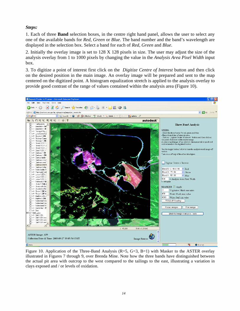
Steps: 1. Each of three Band selection boxes, in the centre right hand panel, allows the user to select any one of the available bands for Red, Green or Blue. The band number and the band’s wavelength are displayed in the selection box. Select a band for each of Red, Green and Blue. 2. Initially the overlay image is set to 128 X 128 pixels in size. The user may adjust the size of the analysis overlay from 1 to 1000 pixels by changing the value in the Analysis Area Pixel Width input box. 3. To digitize a point of interest first click on the Digitize Centre of Interest button and then click on the desired position in the main image. An overlay image will be prepared and sent to the map centered on the digitized point. A histogram equalization stretch is applied to the analysis overlay to provide good contrast of the range of values contained within the analysis area (Figure 10).

Figure 10. Application of the Three-Band Analysis (R=5, G=3, B=1) with Masker to the ASTER overlay illustrated in Figures 7 through 9, over Brenda Mine. Note how the three bands have distinguished between the actual pit area with outcrop to the west compared to the tailings to the east, illustrating a variation in clays exposed and / or levels of oxidation.

15

4. Steps 1 through 3 can be repeated to view any three band combinations selected for Red, Green and Blue. At any point Step 3 initiates the recalculation and display of the area data being analysed. Note: For a Red, Green and Blue image which approaches our visual red, green and blue, users can enter ASTER bands 2, 3, 1 or 5, 3, 1 (R=2,G=3, B=1, or R=5, G=3, B=1). The ASTER images used as the backdrop in the IAT are already displayed using one of these three band combinations. 5. The analysis overlay image may be toggled off and on with the button to compare with features between the two images. If the overlay image disappears, try the button. Button, button, button. 6. As the user moves in or out in scale to observe the results of analysis, the butto button may be used to resample (focus for the screen) information at the new scale. 7. The button opens the prints setup dialog box so a hardcopy printout can be configured. Note: Different bands have different ground sampling dimensions (pixel size, see Table 1). The area of the overlying image analysed “Analysis Area Pixel Width” is a result of the number of pixels chosen (e.g. 128 width by 128 length) by the user. When an analysis is performed all the bands are resampled to a 15 metre resolution. Note: Use the ( ) button to return to the Image Analysis Tools page. To use MASKER:

Operation of the MASKER tool is discussed above under One-Band Analysis. Two-Band Analysis

The Two-Band Ratio Analysis allows the user to generate band ratio analysis images. The ratio between two bands is used to display the variability between two regions of the electromagnetic spectrum across the analysis area. This type of analysis has been used to discriminate many features such as minerals, water clarity, water depth and vegetation vigour. The ratio process also reduces the effect of shadows on the analysis. But the result should be used with caution as the ratio for two materials may be the same even though the actual reflectance spectrum values for the materials are completely different.

The resultant ratio image is stretched using the histogram equalization process to enhance its contrast. Again the assigning of various colour maps to the ratio image may enhance features of interest.

Some commonly employed ratios are: A2/1 iron oxides (ferric iron, Fe³+) A(7+9)/8 carbonate / chlorite / epidote A(5+7)/6 sericite / muscovite / illite / smectite A7/5 kaolinite A11/10 silica

16

These sample ratios are taken from Kalinowski and Oliver (2004). These are only a few examples from an extensive list, with references, of ASTER ratios used in mineral exploration. It is important to remember that the ratios are not absolute. Information derived from ASTER must be ground truthed and will vary from one location to another. If the user is familiar with the geology and ground cover of an area, use that knowledge to experiment to find band ratios (or combinations) which work to isolate and identify information you know. Then that ratio may be used to identify similar materials elsewhere in the image. ASTER information should not be used in isolation, but rather should be used in conjunction with your knowledge and a number of other tools in the field.

Steps: 1. Each of two Band selection boxes, in the centre right hand panel, allows the user to select any of the available bands for Numerator or Denominator in this ratio analysis. The band number and the band’s wavelength are displayed in the selection box. Select a band for each of Numerator and Denominator. If the same band is selected for the numerator and the denominator then a ratio image is not generated but a simple one-band image is presented. 2. There are 41 colour schemes that may be applied to the analysis overlay. Select the desired colour scheme from the Colour Map selection box and re-digitize the area of interest. The various colour maps may be used to highlight features not readily apparent in a grayscale or rainbow coloured image. 3. Initially the overlay image is set to 128 X 128 pixels in size. The user may adjust the size of the analysis overlay from 1 to 1000 pixels by changing the value in the Analysis Area Pixel Width input box. 4. To digitize a point of interest first click on the Digitize Centre of Interest button and then click on the desired position in the main image. An overlay image will be prepared and sent to the map centered on the digitized point. A histogram equalization stretch is applied to the analysis overlay to provide good contrast of the range of values contained within the analysis area. 5. Steps 1 through 4 can be repeated to view any two-band ratio combinations. At any point Step 4 initiates the recalculation and display of the area data being analysed. 6. The analysis overlay image may be toggled off and on with the button to compare with features between the two images. If the overlay image disappears, try the button. Button button button. 7. As the user moves in or out in scale to observe the results of analysis, the ( ) button may be used to resample (focus for the screen) information at the new scale. 8. The button opens the prints setup dialog box so a hardcopy printout can be configured. Note: Different bands have different ground sampling dimensions (pixel size, see Table 1). The area of the overlying image analysed “Analysis Area Pixel Width” is a result of the number of pixels chosen (e.g. 128 width by 128 length) by the user. When an analysis is performed all the bands are resampled to a 15 metre resolution. Note: Use the ( ) button to return to the Image Analysis Tools page.

17

To use MASKER: Operation of the MASKER tool is discussed above under One-Band Analysis.

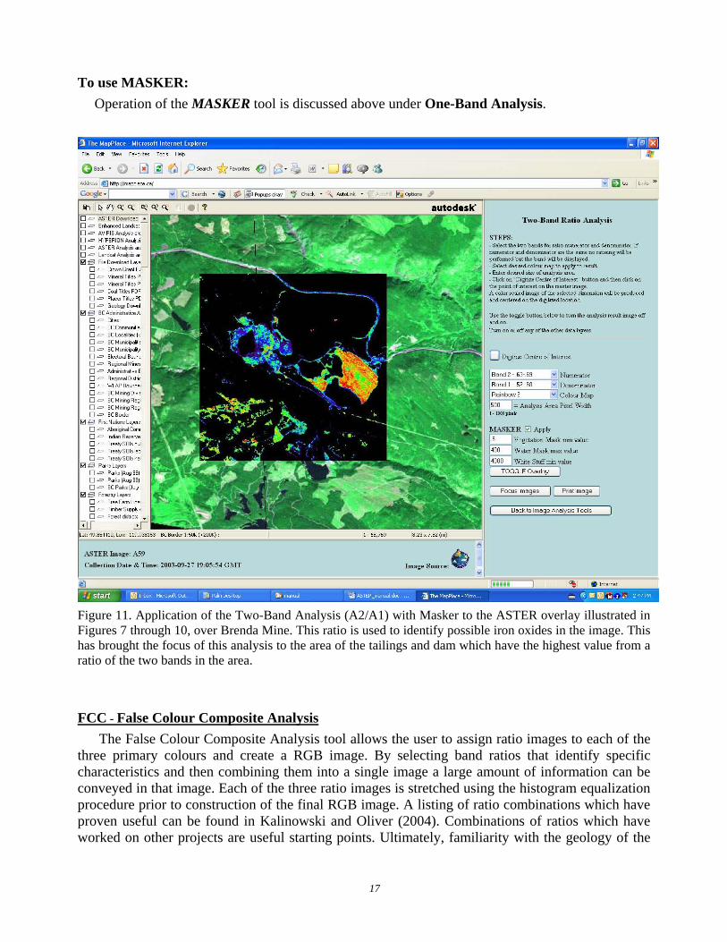
Figure 11. Application of the Two-Band Analysis (A2/A1) with Masker to the ASTER overlay illustrated in Figures 7 through 10, over Brenda Mine. This ratio is used to identify possible iron oxides in the image. This has brought the focus of this analysis to the area of the tailings and dam which have the highest value from a ratio of the two bands in the area.

FCC - False Colour Composite Analysis The False Colour Composite Analysis tool allows the user to assign ratio images to each of the

three primary colours and create a RGB image. By selecting band ratios that identify specific characteristics and then combining them into a single image a large amount of information can be conveyed in that image. Each of the three ratio images is stretched using the histogram equalization procedure prior to construction of the final RGB image. A listing of ratio combinations which have proven useful can be found in Kalinowski and Oliver (2004). Combinations of ratios which have worked on other projects are useful starting points. Ultimately, familiarity with the geology of the

18

area being examined and experimentation may realise a series of ratios which are best suited to discriminate information of interest in an exploration program. Steps: 1. Three pairs of Band selection boxes, in the centre right hand panel, allow the user to select any of the available bands for numerator or denominator in this colour composite analysis. The band number and the band’s wavelength are displayed in each selection box. Select a band for each of a Red Numerator & Red Denominator, Green Numerator & Green Denominator, and Blue Numerator & Blue Denominator. If the same band is selected for both the numerator and the denominator then a ratio image is not generated and the information from that single band is used for the colour it was selected for in the composite analysis. 2. Initially the overlay image is set to 128 X 128 pixels in size. The user may adjust the size of the analysis overlay from 1 to 1000 pixels by changing the value in the Analysis Area Pixel Width input box. 3. To digitize a point of interest first click on the Digitize Centre of Interest button and then click on the desired position in the main image. An overlay image will be prepared and sent to the map centered on the digitized point. A histogram equalization stretch is applied to the analysis overlay to provide good contrast of the range of values contained within the analysis area. 4. Steps 1 through 3 can be repeated to view any False Colour Composite ratio combinations. At any point Step 3 initiates the recalculation and display of the area data being analysed. 5. The analysis overlay image may be toggled off and on with the button to compare with features between the two images. If the overlay image disappears, try the button. Button button button. 7. As the user moves in or out in scale to observe the results of analysis, the ( ) button may be used to resample (focus for the screen) information at the new scale. 8. The button opens the prints setup dialog box so a hardcopy printout can be configured. Note: Different bands have different ground sampling dimensions (pixel size, see Table 1). The area of the overlying image analysed “Analysis Area Pixel Width” is a result of the number of pixels chosen (e.g. 128 width by 128 length) by the user. When an analysis is performed all the bands are resampled to a 15 metre resolution. Note: Use the ( ) button to return to the Image Analysis Tools page. To use MASKER:

Operation of the MASKER tool is discussed above under One-Band Analysis.

19

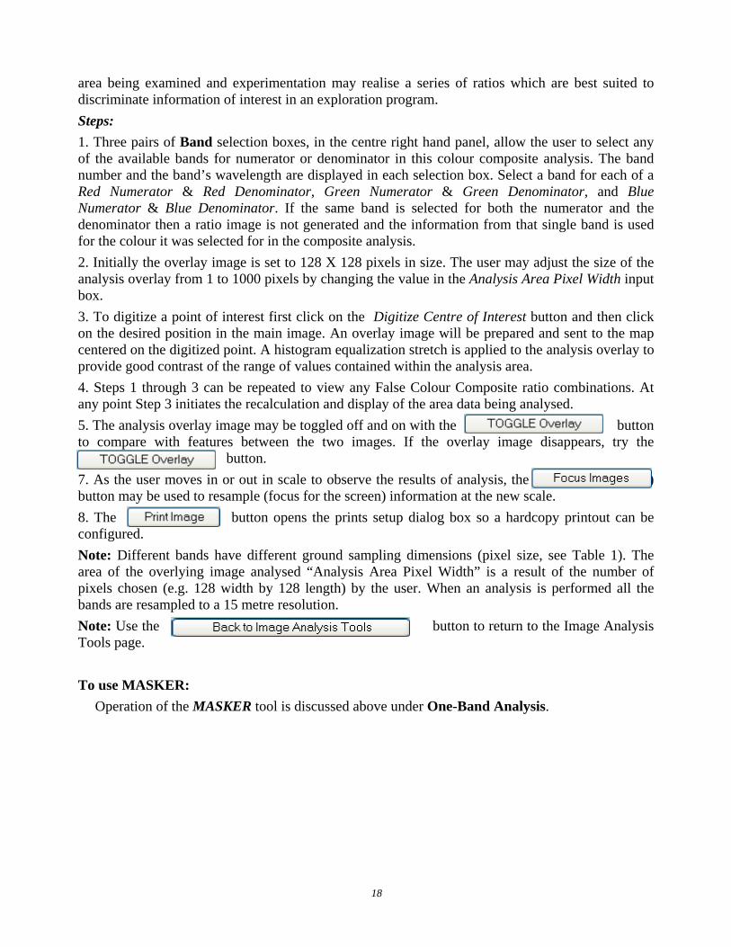
Figure 12. Application of the False Colour Composite Analysis (A4/A2, A4/A5, A5/A6) with Masker to the ASTER overlay illustrated in Figures 7 through 11, over Brenda Mine. This ratio was used to identify possible gossan, alteration and host rock (red, green and blue respectively) in the image overlay area. This has distinguished the host rock (blue) at the mine from the tailings dam to the right. This combination of band ratios is taken from Kalinowski and Oliver (2004).

NDVI Vegetation Analysis

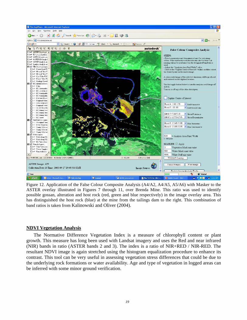
The Normative Difference Vegetation Index is a measure of chlorophyll content or plant growth. This measure has long been used with Landsat imagery and uses the Red and near infrared (NIR) bands in ratio (ASTER bands 2 and 3). The index is a ratio of NIR+RED / NIR-RED. The resultant NDVI image is again stretched using the histogram equalization procedure to enhance its contrast. This tool can be very useful in assessing vegetation stress differences that could be due to the underlying rock formations or water availability. Age and type of vegetation in logged areas can be inferred with some minor ground verification.

20

Steps: 1. Select the desired colour scheme from the Colour Map selection box. There are 41 colour schemes that may be applied to the analysis overlay. The various colour maps may be used to highlight features not readily apparent in a grayscale or rainbow coloured image. 2. Initially the overlay image is set to 128 X 128 pixels in size. The user may adjust the size of the analysis overlay from 1 to 1000 pixels by changing the value in the Analysis Area Pixel Width input box. 3. To digitize a point of interest first click on the Digitize Centre of Interest button and then click on the desired position in the main image. An overlay image will be calculated and sent to the map centered on the digitized point. A histogram equalization stretch is applied to the analysis overlay to provide good contrast of the range of values contained within the analysis area (Figure 13). 4. Steps 1 through 3 can be repeated to view the area of interest using various colour schemes. At any point Step 3 initiates the recalculation and display of the area data being analysed.

Figure 13. Screen view of the NDVI Vegetation Index window illustrating the user input components. The overlay analysis image covers the former Brenda mining operation. Clearly areas of little or no vegetation are in purple to black. Note some probable biological (algae) activity in water of the pit and tailings ponds.

21

5. The analysis overlay image may be toggled off and on with the button to compare with features between the overlay image and original image. If the overlay image disappears, try the button. 6. As the user moves in or out in scale to observe the results of analysis, the ( ) button may be used to resample (focus for the screen) information at the new scale. 7. The button opens the prints setup dialog box so a hardcopy printout can be configured. Note: Different bands have different ground sampling dimensions (pixel size, see Table 1). The area of the overlying image analysed “Analysis Area Pixel Width” is a result of the number of pixels chosen (e.g. 128 width by 128 length) by the user. When an analysis is performed all the bands are resampled to a 15 metre resolution. Note: Use the ( ) button to return to the Image Analysis Tools page. To use MASKER:

Operation of the MASKER tool is discussed above under One-Band Analysis. Tasseled Cap Transformation The Tassled Cap Transformation is a traditional Landsat analysis technique used to compress spectral data into a few bands to reveal key forest attributes. The tool only works on Landsat images.

Spectral Angle Mapper The spectral angle mapper (SAM) generates an analysis image where each pixel contains the

vector angle between a reference spectrum and the spectrum at each pixel location. In the IAT the reference spectrum is selected by the user from a pixel on the reference image. The spectral angle may be calculated for any number of contiguous image bands. This tool requires significant computation effort so the fewer bands and smaller analysis area that are used the quicker the result will be returned. Analysis based on large numbers of image bands could require several minutes to calculate. The best results are often obtained by selecting only the band range that is relevant to the target feature one is attempting to map. Steps: 1. To use the SAM tool the user first must decide on the range of contiguous image bands that will form the spectrum by selecting the maximum and minimum bands of the range. Two Band selection boxes, in the centre right hand panel, allow the user to select any of the available bands for Minimum Band and Maximum Band. The band number and the band’s wavelength are displayed in each selection box. Select these two bands. Two different bands must be selected such that they create sufficient range or the calculation will not be performed. 2. Next, a reference or target spectrum is selected by clicking on the Digitize Target Pixel button and then digitizing a pixel on the reference image that contains the desired reference spectrum. The

22

resulting calculation is quickly performed, so although the lower window may indicate that it is still processing, it is actually waiting for the next components to be selected. 3. At this point the user may also select a colour scheme for the resultant analysis image from the Colour Map selection box. 4. The size of the analysis area may be selected by modifying the value in the Analysis Area Pixel Width entry field. Initially the overlay image is set to 128 X 128 pixels in size. The user may adjust the size of the analysis overlay from 1 to 1000 pixels. 5. Next, the user selects the area to be mapped with the SAM tool by clicking on the Digitize Centre of Interest button and digitizing a location on the reference image. Different areas of the image may be mapped with the same reference spectrum simply by clicking on the Digitize Centre of Interest button in the control panel and then selecting a new position on the reference image. Note: This tool is useful when the user knows what exists at one position and wants to map all the areas with a similar spectral response. The spectrum for a single pixel is the result of the integration of the entire individual spectrum received by the measuring instrument from the pixel area. Therefore pixels which contain only a partial amount of the target substance will still have a smaller spectral angle with the reference spectrum than pixels with none of the target substance so in this way some characteristics can be mapped at the sub pixel level. 6. The analysis overlay image may be toggled off and on with the button to compare with features between the SAM image and original ASTER image. If the overlay image disappears, try the button. 7. As the user moves in or out in scale to observe the results of analysis, the ( ) button may be used to resample (focus for the screen) information at the new scale. 8. The button opens the prints setup dialog box so a hardcopy printout can be configured. Note: Different bands have different ground sampling dimensions (pixel size, see Table 1). The area of the overlying image analysed “Analysis Area Pixel Width” is a result of the number of pixels chosen (e.g. 128 width by 128 length) by the user. When an analysis is performed all the bands are resampled to a 15 metre resolution. Note: Use the ( ) button to return to the Image Analysis Tools page. To use MASKER:

Operation of the MASKER tool is discussed above under One-Band Analysis.

23

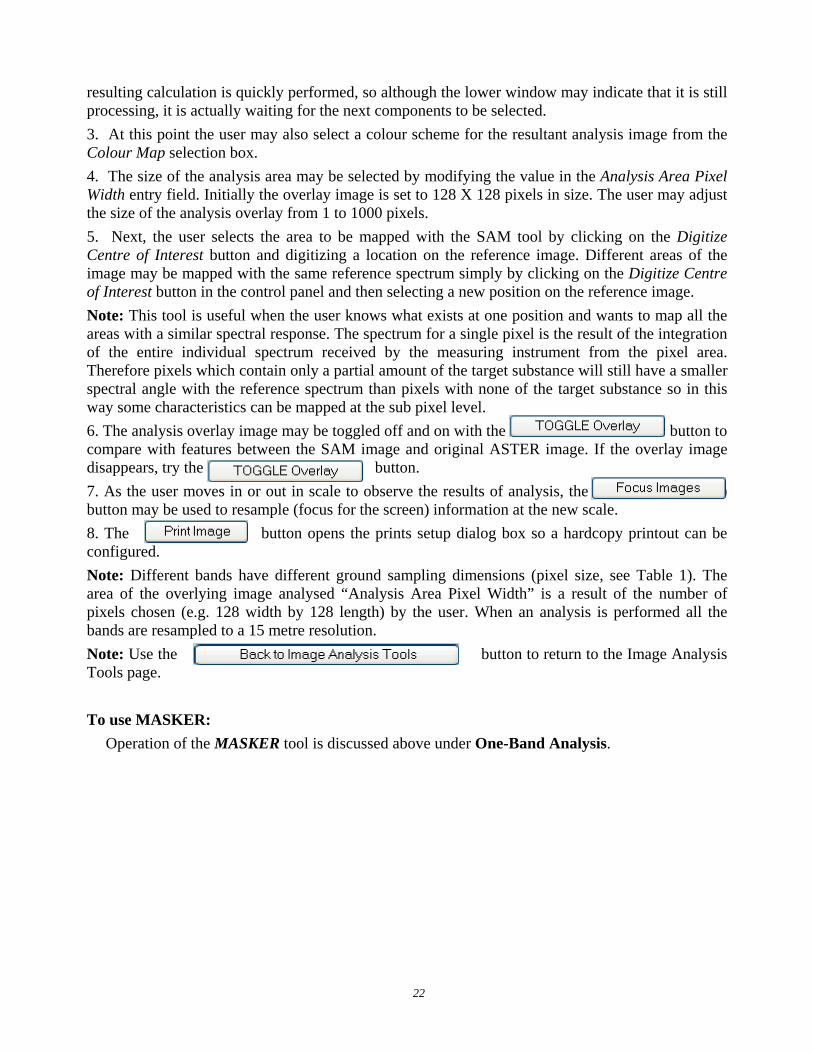
Figure 14. Results of a SAM analysis. The red colours have the smallest spectral angle with the reference spectrum that was obtained from the rectangular logging cut block in the upper left corner of the image overlay. The reference spectrum represented a mix of vegetation and soil. A similar mix/spectrum can be found along either side of the main highway and on many roads around the mine. The overlay analysis image covers the former Brenda mining operation.

Prepared Images The following four selections from the Image Analysis Tools Index Page do not perform an

analysis on the image but rather launch new displays related to the selected ASTER image. Anaglyph Map

An anaglyph (àn´e-glîf´) is a picture or image consisting of two slightly different perspectives of the same subject in contrasting colors that are superimposed on each other, producing a three-dimensional effect when viewed through two correspondingly colored filters.

24

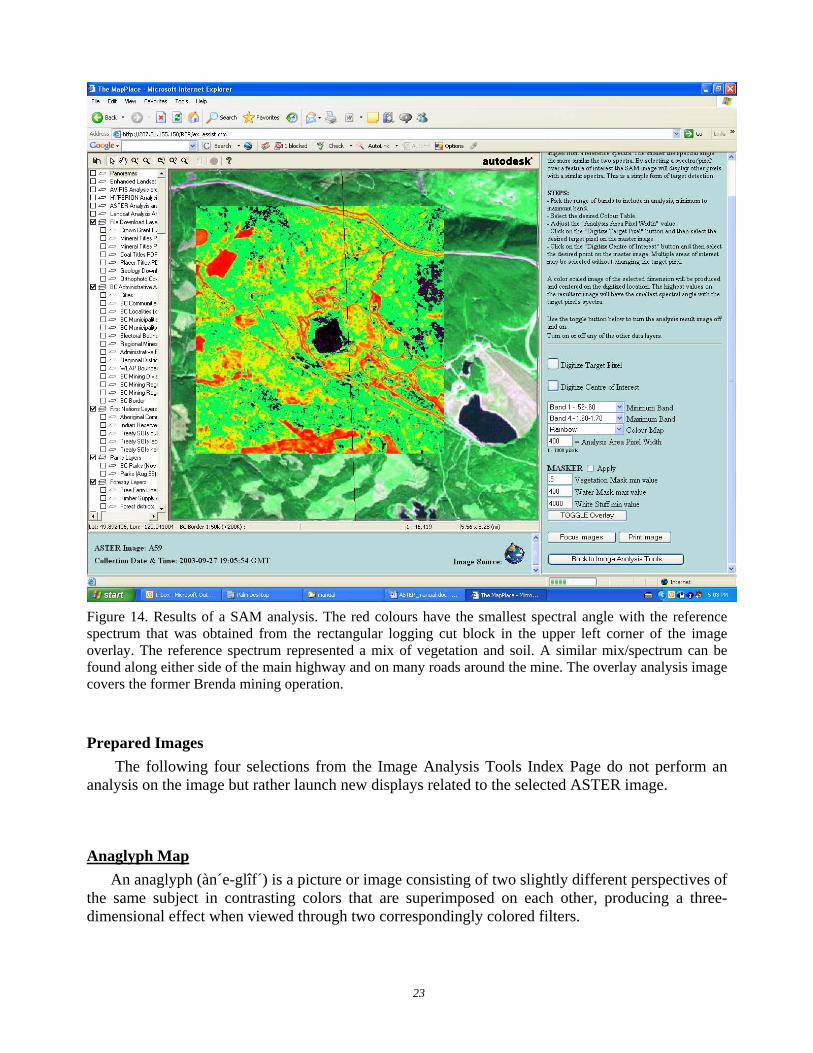
The Anaglyph Map button will launch a new MapPlace map with an ASTER anaglyph image of the user’s selected image forming the main display. The image may be used as any map, or image, as a base in the MapPlace. These maps are rotated so that the satellite flight line is horizontal in the display making map north to the right of the display. This aligns the viewer’s eyes with the flight path and allows viewing of the image in 3D. Anaglyph glasses are required to view the image. Glasses with red and cyan lenses are preferred but red and blue lenses will work reasonably as well. All available MapPlace layers can be overlain on these maps just as with any other MapPlace map. These images have been orthorectifed and fit the existing TRIM base map data very well. 3D topographic surface views such as these provide an excellent tool for interpretation of surficial and bedrock geological features.

Figure 15. The anaglyph map of ASTER image A59. The Brenda Mine and tailings ponds are in the lower left corner of the image (southeast corner).

25

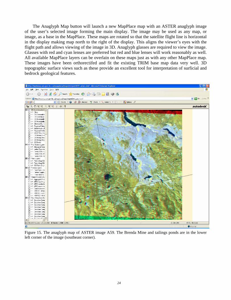
Figure 16. Detail of the lower left corner of the image in Figure 15. Use anaglyph glasses to see the three-dimensional aspect of the terrain and site of Brenda Mine. Virtual Reality

The Virtual Reality button will call a low resolution virtual reality file of the user’s ASTER scene draped over its DEM. If the user has a virtual reality viewer linked to their browser it will be launched and the file immediately viewable. If no virtual reality viewer is linked then the user has the option to save the file for later viewing.

Virtual Reality files (WRL format) have been produced for each image by draping the near-natural colour image over the DEM generated during the orthorectification process. When viewed with the appropriate viewing software these files allow the user to fly through the terrain, generate perspective views and even incorporate new flight paths and viewpoints. Similar functions are available through the Google Earth products discussed below but the virtual reality files provided here are available on a much more detailed topographic base than presently available through Google Earth.

The files have been prepared in two resolutions; the high resolution version is available through the download (see Download Page) option while the low resolution version is available by direct

26

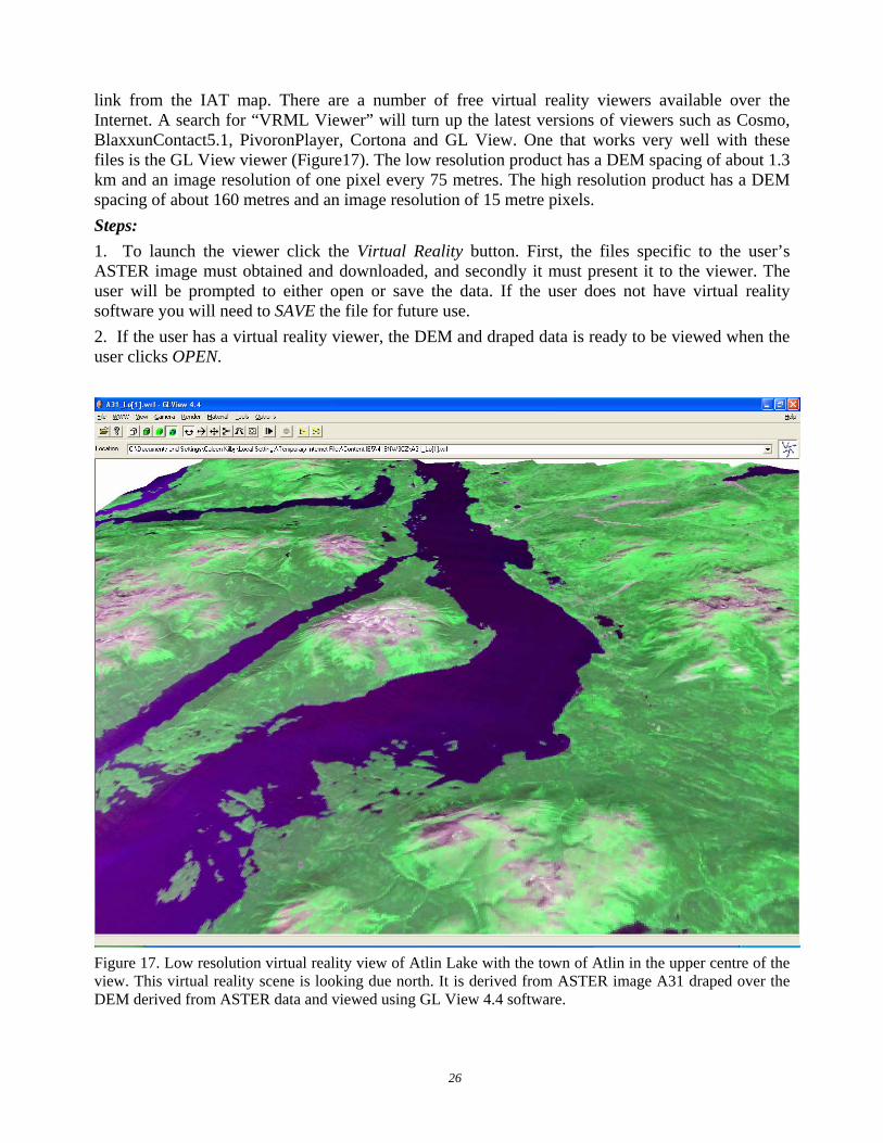
link from the IAT map. There are a number of free virtual reality viewers available over the Internet. A search for “VRML Viewer” will turn up the latest versions of viewers such as Cosmo, BlaxxunContact5.1, PivoronPlayer, Cortona and GL View. One that works very well with these files is the GL View viewer (Figure17). The low resolution product has a DEM spacing of about 1.3 km and an image resolution of one pixel every 75 metres. The high resolution product has a DEM spacing of about 160 metres and an image resolution of 15 metre pixels. Steps: 1. To launch the viewer click the Virtual Reality button. First, the files specific to the user’s ASTER image must obtained and downloaded, and secondly it must present it to the viewer. The user will be prompted to either open or save the data. If the user does not have virtual reality software you will need to SAVE the file for future use. 2. If the user has a virtual reality viewer, the DEM and draped data is ready to be viewed when the user clicks OPEN.

Figure 17. Low resolution virtual reality view of Atlin Lake with the town of Atlin in the upper centre of the view. This virtual reality scene is looking due north. It is derived from ASTER image A31 draped over the DEM derived from ASTER data and viewed using GL View 4.4 software.

27

3. At this point the virtual reality file will open in a new window. Each virtual reality viewer will have different commands, and it is recommended that the user familiarize themselves with the use of their viewer (by testing, or by reading a manual). In most viewers the image may likely begin with a black DEM. The draped image will need to be made visible (e.g. commands in GL View are Camera, then Head Light). And, as it is desirable to start with a view of the entire image, the user may need to backout to see the full DEM (e.g. this command in GL View is Reset camera). Various commands will allow the user to make full use of the virtual reality file to assist or enhance their work with the ASTER image(s) of interest. 4. If greater resolution is of interest the high resolution version is available through the Download Page option discussed below. Google Earth

The Google Earth button will launch the Google Earth package for the selected ASTER image on the client’s computer if they have Google Earth loaded. If they do not have Google Earth loaded they have the option of saving the file for later viewing. Use of Google Earth requires a relatively fast Internet connection and computer. The new Google Earth viewer provides powerful viewing capabilities with the ability to incorporate external data. Several of the ASTER products such as the near-natural colour image, anaglyph image and alteration mineral images have been incorporated into Google Earth files that are accessible through the MapPlace and provide an enhanced level of data viewing.

The Google Earth free viewer provides a significant advance in viewing geospatial information over the Internet. A Google Earth display is available for each ASTER image (Figure 18). Each display includes (in the following order);

- The ASTER image footprint - an anaglyph image - a near-natural colour image - an iron oxide image - a siliceous rock image - a sericte-illite image - an alunite-kaolinite image and other imagery and spatial data available from Google Earth. All project information displayed through Google Earth is also available through the MapPlace.

Steps: 1. The Google Earth display can be accessed (downloaded) by clicking on the Google Earth button of the ASTER IAT tool selection panel (Figure 6). The Google Earth sphere will spin into your viewing window and position itself centered on the ASTER image the user has previously selected. 2. Two panels appear along the left and below the viewing window. In the centre of the left hand panel is the area for listing of Temporary Places. Below this is a listing of the ASTER data which is available for viewing. Click on the arrow to the left of the box for ASTER # Full Download where the # symbol is replaced by the numeral for the selected ASTER image (a number between 1 and 139). If the box is clicked an entire download of all the material for that image will be initiated and greatly slow access to the site. If this occurs, click the box a second time.

28

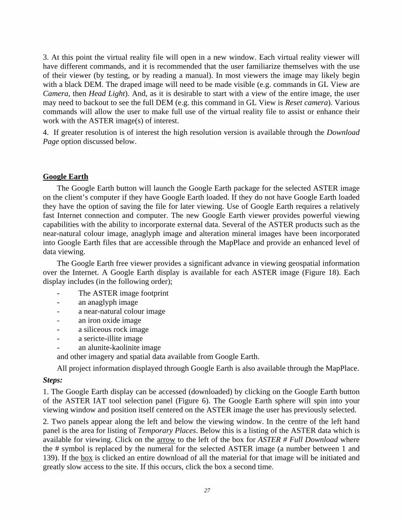
3. Seven options will be listed for the selected ASTER image (listed above). Click the box for A# ASTER Image to download the image itself onto the Google globe. A red square will appear in the viewing window with the word “Loading”. WAIT while the image is loaded (Figure 18).

Figure 18. A Google Earth view of the area of ASTER A31, Atlin Lake in northwestern BC. In this view the ASTER image is being loaded. The tilted white square is the footprint of the ASTER image. 4. The Google Earth viewer allows the user to turn the various images off and on and adjust the opacity of a selected image. The user must familiarize themselves with all the capabilities of the Google Earth viewer to achieve the maximum use out of this tool. Using the control in the lower panel and / or the mouse one can move in and take a closer look at the information provided by the ASTER multispectral image in relation to the physical aspect of a site. Figure 19 is a view of the Atlin area with the ASTER near-natural colour image. 5. Four Alteration-Mineral images are included in Google Earth for each ASTER image. See discussion of these images below under Download Page. To view one of these derivative overlays, find the list in the left hand panel and check the box next to the alteration of interest. In Figure 20 the ASTER image for sericite-illite has been overlain over the Google Earth view of the Atlin area.

29

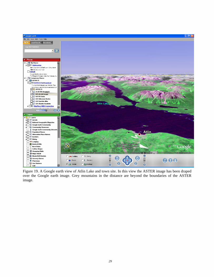
Figure 19. A Google earth view of Atlin Lake and town site. In this view the ASTER image has been draped over the Google earth image. Grey mountains in the distance are beyond the boundaries of the ASTER image.

30

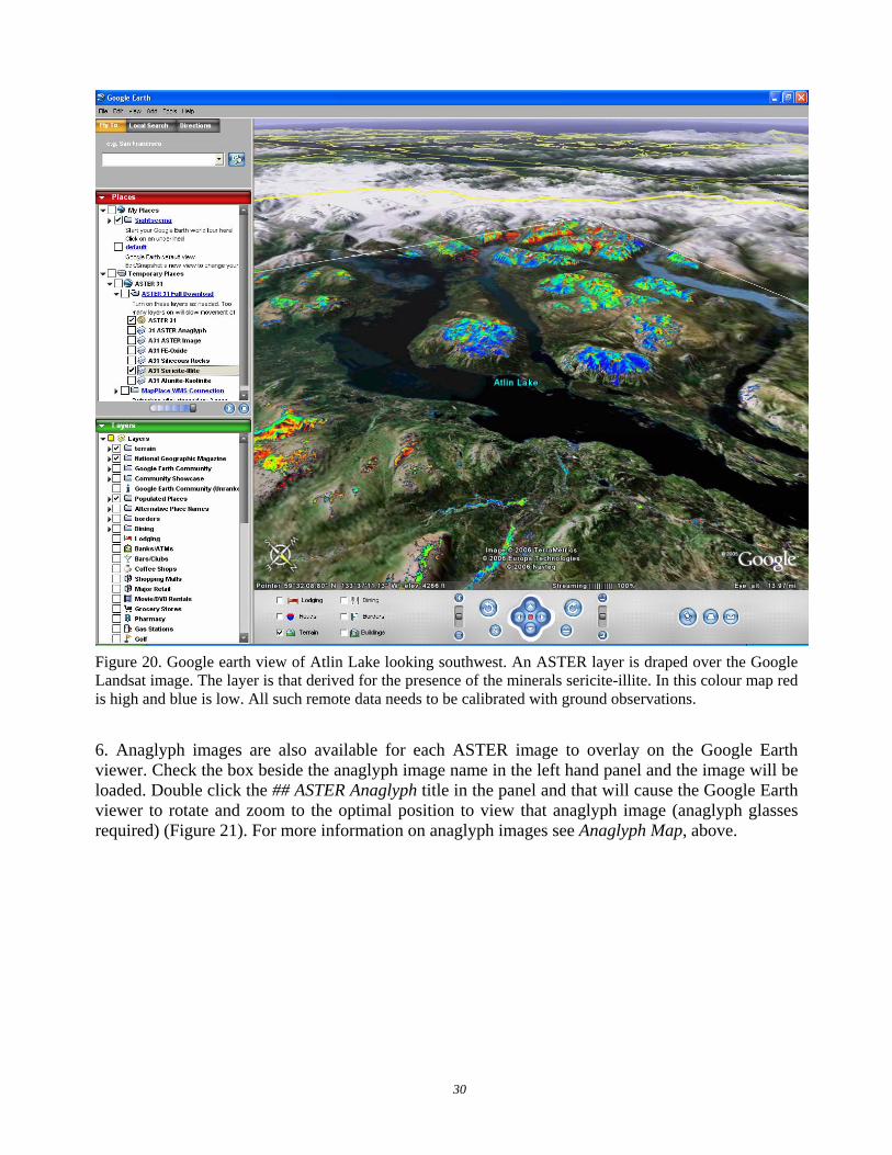
Figure 20. Google earth view of Atlin Lake looking southwest. An ASTER layer is draped over the Google Landsat image. The layer is that derived for the presence of the minerals sericite-illite. In this colour map red is high and blue is low. All such remote data needs to be calibrated with ground observations. 6. Anaglyph images are also available for each ASTER image to overlay on the Google Earth viewer. Check the box beside the anaglyph image name in the left hand panel and the image will be loaded. Double click the ## ASTER Anaglyph title in the panel and that will cause the Google Earth viewer to rotate and zoom to the optimal position to view that anaglyph image (anaglyph glasses required) (Figure 21). For more information on anaglyph images see Anaglyph Map, above.

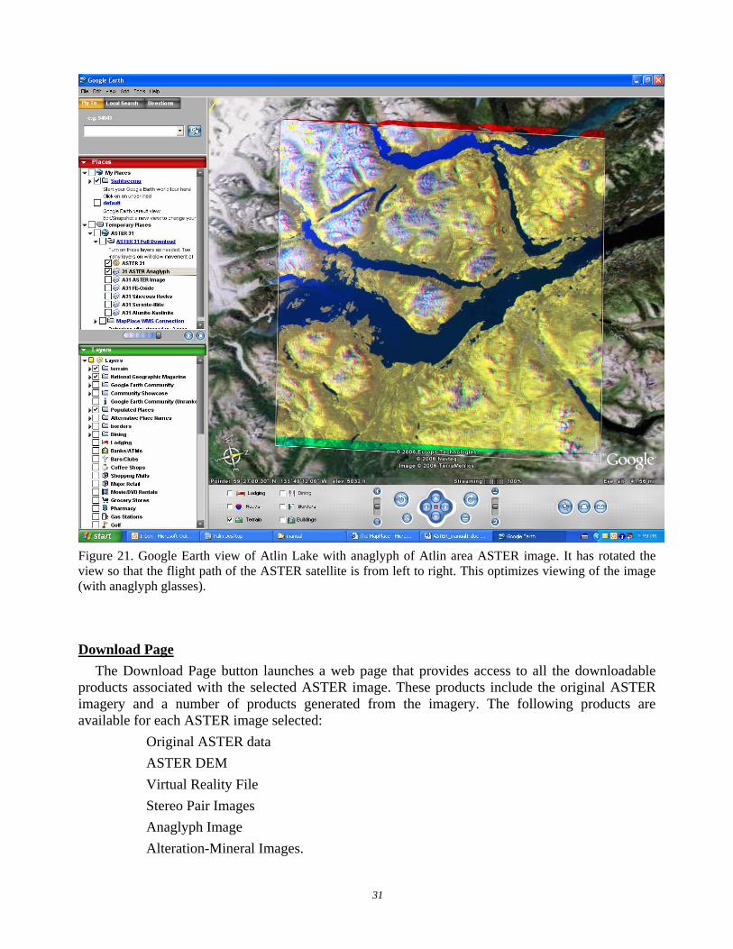
31

Figure 21. Google Earth view of Atlin Lake with anaglyph of Atlin area ASTER image. It has rotated the view so that the flight path of the ASTER satellite is from left to right. This optimizes viewing of the image (with anaglyph glasses). Download Page

The Download Page button launches a web page that provides access to all the downloadable products associated with the selected ASTER image. These products include the original ASTER imagery and a number of products generated from the imagery. The following products are available for each ASTER image selected:

Original ASTER data ASTER DEM Virtual Reality File Stereo Pair Images Anaglyph Image Alteration-Mineral Images.

32

Each of these files is described below with additional information available on the download page and also may be discussed elsewhere in this manual. Steps: 1. Click on the Download Page button in the ASTER IAT tool selection panel. 2. Select the image or file of interest and click on the image title (as listed above). The exception to this is for ASTER DEM where the user must choose one of the two formats in which to download the DEM and clicks on one of these choices (GeoTiff or USGS DEM). The choice will depend on the software the user intends to utilize with this data.

Original ASTER Data The ASTER image data, in its original format, can be downloaded for free by the user. The two

original files associated with each image have been zipped together for convenience of handling but are otherwise in the original XML and HDF formats. A search of the Internet will return a large number of free and high end programs capable of manipulating this image format. This data has not been processed.

The 39 previously existing ASTER images and 100 new images included in the IAT have been processed to relative reflectance values. Until 2006 ASTER images available on the MapPlace had only been processed to uncalibrated radiance integer (DN) values. ASTER images processed to relative reflectance are available for download from the Exploration Assistant Tools main page in the left hand panel, at the top under ASTER Download.

ASTER DEM During the orthorectification process a relative digital elevation model was constructed. This

model is available for download. The model resolution is 30 metres. Unlike many DEMs where the grid points are interpolated from widely spaced data points this model was generated by a calculation based on the Band 3N (Nadir) and Band 3B (Back-looking) images at each grid point. The DEM is relative and has not been corrected to true elevations. A correction could be applied by the user if desired but for most applications the relative model is adequate.

Many of the ASTER images contain some cloud cover and the elevation of the cloud tops is what is recorded in the DEM rather than the ground elevation. Also, in some images certain pixels in Band 3N or BAND 3B were saturated and resulted in no elevation calculation being possible. These appear as holes in the DEM. This problem usually occurs over very large bright objects such as glaciers.

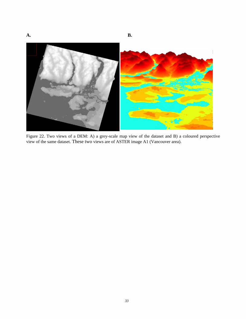
The DEM is provided in two standard DEM formats, USGS DEM and GeoTiff, which can be read by a large number of free and widely available software packages. Figure 22 contains two views of an ASTER image downloaded in USGS DEM format and created using AsterDTM software (SulSoft, 2005).

33

A. B.

Figure 22. Two views of a DEM: A) a grey-scale map view of the dataset and B) a coloured perspective view of the same dataset. These two views are of ASTER image A1 (Vancouver area).

34

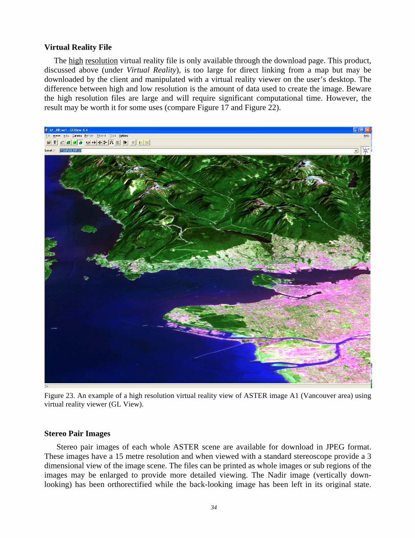
Virtual Reality File The high resolution virtual reality file is only available through the download page. This product,

discussed above (under Virtual Reality), is too large for direct linking from a map but may be downloaded by the client and manipulated with a virtual reality viewer on the user’s desktop. The difference between high and low resolution is the amount of data used to create the image. Beware the high resolution files are large and will require significant computational time. However, the result may be worth it for some uses (compare Figure 17 and Figure 22).

Figure 23. An example of a high resolution virtual reality view of ASTER image A1 (Vancouver area) using virtual reality viewer (GL View).

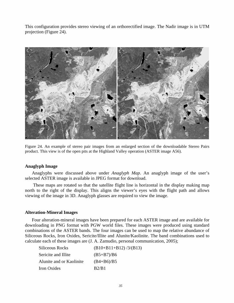
Stereo Pair Images Stereo pair images of each whole ASTER scene are available for download in JPEG format.

These images have a 15 metre resolution and when viewed with a standard stereoscope provide a 3 dimensional view of the image scene. The files can be printed as whole images or sub regions of the images may be enlarged to provide more detailed viewing. The Nadir image (vertically down-looking) has been orthorectified while the back-looking image has been left in its original state.

35

This configuration provides stereo viewing of an orthorectified image. The Nadir image is in UTM projection (Figure 24).

Figure 24. An example of stereo pair images from an enlarged section of the downloadable Stereo Pairs product. This view is of the open pits at the Highland Valley operation (ASTER image A56).

Anaglyph Image

Anaglyphs were discussed above under Anaglyph Map. An anaglyph image of the user’s selected ASTER image is available in JPEG format for download.

These maps are rotated so that the satellite flight line is horizontal in the display making map north to the right of the display. This aligns the viewer’s eyes with the flight path and allows viewing of the image in 3D. Anaglyph glasses are required to view the image.

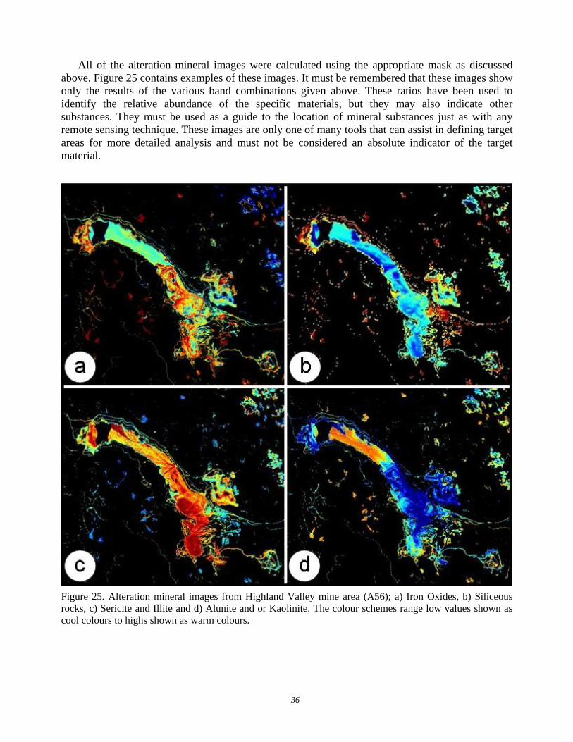
Alteration-Mineral Images Four alteration-mineral images have been prepared for each ASTER image and are available for

downloading in PNG format with PGW world files. These images were produced using standard combinations of the ASTER bands. The four images can be used to map the relative abundance of Siliceous Rocks, Iron Oxides, Sericite/Illite and Alunite/Kaolinite. The band combinations used to calculate each of these images are (J. A. Zamudio, personal communication, 2005);

Siliceous Rocks (B10+B11+B12) /3/(B13) Sericite and Illite (B5+B7)/B6 Alunite and or Kaolinite (B4+B6)/B5 Iron Oxides B2/B1

36

All of the alteration mineral images were calculated using the appropriate mask as discussed above. Figure 25 contains examples of these images. It must be remembered that these images show only the results of the various band combinations given above. These ratios have been used to identify the relative abundance of the specific materials, but they may also indicate other substances. They must be used as a guide to the location of mineral substances just as with any remote sensing technique. These images are only one of many tools that can assist in defining target areas for more detailed analysis and must not be considered an absolute indicator of the target material.

Figure 25. Alteration mineral images from Highland Valley mine area (A56); a) Iron Oxides, b) Siliceous rocks, c) Sericite and Illite and d) Alunite and or Kaolinite. The colour schemes range low values shown as cool colours to highs shown as warm colours.

37

ACKNOWLEDGEMENTS This manual has been written by Caleen Kilby and Ward Kilby of Cal Data Ltd. This project

was made possible by a grant from Geoscience BC, and funding for two previous projects from AME BC under the Rocks to Riches Program. The British Columbia Ministry of Energy, Mines and Petroleum Resources provided support in the form of Internet hosting of the project products on the MapPlace web site. The authors would like to thank Dr. Joe Zamudio for his useful suggestions regarding multispectral analysis.

We would like to thank Larry Jones and Patrick Desjardins of the British Columbia Geological Survey, Ministry of Energy, Mines and Petroleum Resources, for invaluable assistance in providing information and access to the MapPlace website.

REFERENCES

Google (2005): Google Earth, Global Internet viewer of imagery and vector information; URL http://earth.google.com

ImSpec (2004): ACORN5, Atmospheric correction software package. Ver 040801, URL www.imspec.com

Kalinowski, A. and S. Oliver (2004): ASTER Mineral Index Processing Manual, Remote Sensing Applications, Geoscience Australia, October 2004, URL http://www.ga.gov.au/image_cache/GA7833.pdf

Kilby, W.E., Kliparchuk, K., and McIntosh, A. (2004): Image Analysis Toolbox and Enhanced Satellite Imagery Integrated into the MapPlace; British Columbia Ministry of Energy and Mines, Geological Fieldwork 2003, Paper 2004-1, p.209-215, URL www.em.gov.bc.ca/DL/GSBPubs/GeoFldWk/2003/20-Kilby-209-216-w.pdf

Kilby, W.E. (2005): MapPlace.ca Image Analysis Toolbox – Phase 2; British Columbia Ministry of Energy and Mines, Geological Fieldwork 2004, Paper 2005-1, p.231-235, URL www.em.gov.bc.ca/DL/GSBPubs/GeoFldWk/2004/PaperRR05.pdf

Lillesand, T.M. and Kieffer, R.W. (2000): Remote Sensing and Image Interpretation; 4th ed., Wiley, New York, 724 pages.

NASA Jet Propulsion Laboratory (2000): ASTER Spectral Library, On-line spectral library. URL http://speclib.jpl.nasa.gov/Search.htm

NASA Jet Propulsion Laboratory (2005): Lat/Long Adjustment Tool, ASTER spatial location correction service access page. URL http://asterweb.jpl.nasa.gov/latlon.asp

NASA MODIS Atmosphere (2005): Daily Atmospheric Water Vapour Mean display, On-line display of daily MODIS derivative product images. URL http://modis-atmos.gsfc.nasa.gov/index.html

RSI (2005): ENVI, Image analysis software package. Ver 4.2, URL www.rsinc.com/envi

SulSoft (2005): AsterDTM, ASTER orthorectification software. Ver 2.2, URL www.envi.com.br/asterdtm

Vincent, R.K. (1997): Fundamentals of Geological and Environmental Remote Sensing; Prentice Hall, Upper Saddle River, NJ, 366 pages.