Embed Size (px)
Citation preview

Examining Ambiguities in the Automatic Packet Reporting System
A Thesis
Presented to
the Faculty of California Polytechnic State University
San Luis Obispo
In Partial Fulfillment
of the Requirements for the Degree
Master of Science in Electrical Engineering
by
Kenneth W. Finnegan
December 2014

© 2014
Kenneth W. Finnegan
ALL RIGHTS RESERVED
ii
COMMITTEE MEMBERSHIP
TITLE: Examining Ambiguities in the AutomaticPacket Reporting System
AUTHOR: Kenneth W. Finnegan
DATE SUBMITTED: December 2014
REVISION: 1.2
COMMITTEE CHAIR: Bridget Benson, Ph.D.Assistant Professor, Electrical Engineering
COMMITTEE MEMBER: John Bellardo, Ph.D.Associate Professor, Computer Science
COMMITTEE MEMBER: Dennis Derickson, Ph.D.Department Chair, Electrical Engineering
iii
ABSTRACT
Examining Ambiguities in the Automatic Packet Reporting System
Kenneth W. Finnegan
The Automatic Packet Reporting System (APRS) is an amateur radio packet network
that has evolved over the last several decades in tandem with, and then arguably beyond,
the lifetime of other VHF/UHF amateur packet networks, to the point where it is one of
very few packet networks left on the amateur VHF/UHF bands. This is proving to be
problematic due to the loss of institutional knowledge as older amateur radio operators
who designed and built APRS and other AX.25-based packet networks abandon the hobby
or pass away. The purpose of this document is to collect and curate a sufficient body of
knowledge to ensure the continued usefulness of the APRS network, and re-examining the
engineering decisions made during the network’s evolution to look for possible improvements
and identify deficiencies in documentation of the existing network.
iv
TABLE OF CONTENTS
List of Figures vii
1 Preface 1
2 Introduction 32.1 History of APRS . . . . . . . . . . . . . . . . . . . . . . . . . . . . . . . . . 42.2 Physical Topology and Hardware . . . . . . . . . . . . . . . . . . . . . . . . 5
2.2.1 Station Block Diagrams . . . . . . . . . . . . . . . . . . . . . . . . . 62.3 Document Overview . . . . . . . . . . . . . . . . . . . . . . . . . . . . . . . 8
I OSI Layer 1 — Physical 10
3 Amateur Bell 202 113.1 Bell 202 in Amateur Radio . . . . . . . . . . . . . . . . . . . . . . . . . . . 123.2 Amateur Bell 202 Transmission Format . . . . . . . . . . . . . . . . . . . . 13
3.2.1 Excluding HDLC from Layer 2 AX.25 . . . . . . . . . . . . . . . . . 153.2.2 Calculating the Frame Check Sum . . . . . . . . . . . . . . . . . . . 16
3.3 FM Deviation and Emphasis . . . . . . . . . . . . . . . . . . . . . . . . . . 183.4 Carrier Sense Multiple Access . . . . . . . . . . . . . . . . . . . . . . . . . . 203.5 Conclusion . . . . . . . . . . . . . . . . . . . . . . . . . . . . . . . . . . . . 22
4 KISS 244.1 Isolating Modulation from Network . . . . . . . . . . . . . . . . . . . . . . . 254.2 Shortcomings of KISS . . . . . . . . . . . . . . . . . . . . . . . . . . . . . . 254.3 Conclusion . . . . . . . . . . . . . . . . . . . . . . . . . . . . . . . . . . . . 27
II OSI Layer 2 — Data Link 28
5 AX.25 295.1 Header Format for APRS . . . . . . . . . . . . . . . . . . . . . . . . . . . . 29
5.1.1 TNC Description / Destination Address . . . . . . . . . . . . . . . . 305.1.2 Source Address . . . . . . . . . . . . . . . . . . . . . . . . . . . . . . 305.1.3 Routing Path . . . . . . . . . . . . . . . . . . . . . . . . . . . . . . . 315.1.4 Control Flags . . . . . . . . . . . . . . . . . . . . . . . . . . . . . . . 315.1.5 Protocol IDentifier . . . . . . . . . . . . . . . . . . . . . . . . . . . . 315.1.6 Information Field . . . . . . . . . . . . . . . . . . . . . . . . . . . . . 32
5.2 FCC Identification Requirements . . . . . . . . . . . . . . . . . . . . . . . . 32
v
6 Digital Repeater Routing Behavior 346.1 Routing Aliases . . . . . . . . . . . . . . . . . . . . . . . . . . . . . . . . . . 356.2 Examples . . . . . . . . . . . . . . . . . . . . . . . . . . . . . . . . . . . . . 366.3 Deduplication Behavior . . . . . . . . . . . . . . . . . . . . . . . . . . . . . 386.4 Deprecation of RELAY . . . . . . . . . . . . . . . . . . . . . . . . . . . . . . 396.5 Minimum WIDEn-N Behavior . . . . . . . . . . . . . . . . . . . . . . . . . . 416.6 Variations on Digipeater Behavior . . . . . . . . . . . . . . . . . . . . . . . 42
III OSI Layer 3 — Network 44
7 Node Beaconing Behavior 457.1 Beaconing Algorithms . . . . . . . . . . . . . . . . . . . . . . . . . . . . . . 45
7.1.1 Fixed Interval Beaconing . . . . . . . . . . . . . . . . . . . . . . . . 467.1.2 Time Slot Interval Beaconing . . . . . . . . . . . . . . . . . . . . . . 467.1.3 Nice Interval Beaconing . . . . . . . . . . . . . . . . . . . . . . . . . 487.1.4 Dithered Interval Beaconing . . . . . . . . . . . . . . . . . . . . . . . 487.1.5 SmartBeaconing . . . . . . . . . . . . . . . . . . . . . . . . . . . . . 49
7.2 Path Recommendations . . . . . . . . . . . . . . . . . . . . . . . . . . . . . 517.2.1 Vehicles and Mobile Stations . . . . . . . . . . . . . . . . . . . . . . 547.2.2 Fixed Stations . . . . . . . . . . . . . . . . . . . . . . . . . . . . . . 547.2.3 Airborne Stations . . . . . . . . . . . . . . . . . . . . . . . . . . . . 557.2.4 Proportional Pathing . . . . . . . . . . . . . . . . . . . . . . . . . . . 55
7.3 Conclusion . . . . . . . . . . . . . . . . . . . . . . . . . . . . . . . . . . . . 57
8 APRS RF Channel Capacity 588.1 Network Capacity Objectives . . . . . . . . . . . . . . . . . . . . . . . . . . 598.2 Poisson Channel . . . . . . . . . . . . . . . . . . . . . . . . . . . . . . . . . 598.3 Deficiencies of the Poisson Model . . . . . . . . . . . . . . . . . . . . . . . . 62
9 Conclusion 65
Bibliography 67
Appendices
A Reference CRC-16-CCITT Implementation 70
B SLottime Justification 73
vi
LIST OF FIGURES
2.1 Example packet path from a handheld APRS tracker . . . . . . . . . . . . . 62.2 Block diagram for typical APRS tracker . . . . . . . . . . . . . . . . . . . . 62.3 Block diagram for typical APRS Digipeater . . . . . . . . . . . . . . . . . . 72.4 Block diagram for typical APRS Internet Gateway . . . . . . . . . . . . . . 72.5 The OSI network model as applied to APRS in this paper . . . . . . . . . . 8
3.1 This paper refers to the entirety of OSI Layer 1 as “Amateur Bell 202” . . . 123.2 Amateur Bell 202 signal representing the ASCII letter A (0x41) . . . . . . . 133.3 Amateur Bell 202/HDLC frame format . . . . . . . . . . . . . . . . . . . . . 133.4 Modified AX.25 packet format excluding HDLC fields. . . . . . . . . . . . . 163.5 Algorithm to calculate CRC-16-CCITT in reverse-bit order. . . . . . . . . . 163.6 Pathway of frame payload to final bit stream using only a LSb-first modulator 173.7 Allowable skew in a basic 3002 telephone channel . . . . . . . . . . . . . . . 20
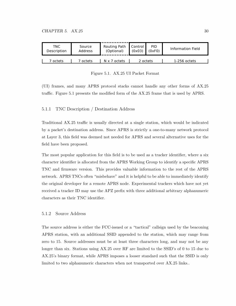
5.1 AX.25 UI Packet Format . . . . . . . . . . . . . . . . . . . . . . . . . . . . . 30
6.1 APRS network used for path routing examples . . . . . . . . . . . . . . . . 36
7.1 Beacon interval dithering algorithm . . . . . . . . . . . . . . . . . . . . . . . 487.2 Original HamHUD SmartBeaconing documentation using C-like syntax . . 527.3 Novel presentation of SmartBeaconing algorithm by the author . . . . . . . 53
8.1 Poisson channel traffic and throughput . . . . . . . . . . . . . . . . . . . . . 61
vii
1 Preface
Like any major research endeavor, this thesis certainly didn’t start anywhere near where
it ended. Most of the credit for the genesis for this thesis needs to be given to Sivan
Toledo, 4X6IZ, from Tel-Aviv University. In 2012 he wrote an article in the amateur radio
QEX technical journal where he explored improving the soundcard digital signal processing
modem used for amateur packet radio by passing the original signals through a series of
band-pass filters [31]. His improvements were commendable, and his article was very well
written, but what bothered me was that more than three decades after the inception of
amateur packet radio, we are still seeing measurable improvement in the modems we use
for the original modulation techniques.
This thesis started with me wanting to tear apart the current state of the various Bell 202
modems used in amateur radio, build a quantitative model of the kinds of interference and
distortion that each modem handled well, and hopefully design a new signal processing
algorithm that showed immunity to the most common forms of interference on real-world
channels. Sevan’s work in JAVA showed promise, but while his library is useful on desktop
computers and Android devices, it left out in the cold the many different 8, 16, and 32 bit
fixed-point microcontrollers that are often used for embedded modems in amateur radio
projects.
As I started to examine the specifications for the various network layers used in the amateur
Automatic Packet Reporting System (namely Bell 202, AX.25, and APRS), I grew increas-
ingly shocked and confused when I kept finding that the documentation I was looking for
was poorly written or simply didn’t exist. Protocol specifications would identify variables
critical for network performance, and then never give guidance on what the actual value
should be. Many of the documents on the expected behavior for network nodes consist
solely of console commands to be run on specific pieces of discontinued hardware instead
1
CHAPTER 1. PREFACE 2
of actual protocol behavior. Most articles discussing aspects of the network disagreed with
other documentation on specific details, and was often internally inconsistent as well.
The final turning point was an interview in March, 2014 with Scott Miller, the designer for
Open Trackers, which are one of the more popular lines of contemporary modems used in
the APRS network. I brought a laundry list of inconsistencies from the network specs and
he explained how much effort he had put into reverse engineering the existing hardware. It
was an eye-opening conversation that drove home how much the amateur packet network
has grown haphazardly over the past three decades into a jumble of band-aids applied upon
band-aids.
I realized that the most important academic research on the topic of APRS isn’t how to
squeeze out another incremental improvement in one of the modem DSP algorithms, but
an over-arching prolegomenon on the entire network stack as it actually exists today. The
existing documentation clearly falls short, and much of the institutional knowledge that
I’ve been able to draw on during my research is coming from the “old guard” of the hobby,
which leaves us exposed to the labor intensive requirement of newcomers to the network to
reverse engineer the existing network before they can participate.
Ideally, this document would be able to stand by itself as a complete “implementer’s guide
to APRS” from the physical layer all the way up to high level aggregate network behavior,
but the scope of reverse engineering that much behavior, documenting it, and then verifying
the documentation quickly becomes monumental. It is my hope that this document does at
least identify the most glaring short-falls in the current documentation and network design,
and gives answers to the questions that can be answered while staying within the scope of
this survey.
For every identified problem which is answered in this paper, there are twice as many
unanswered questions which each warrant being considered as a thesis of their own.
2 Introduction
The Automatic Packet Reporting System (APRS) is an amateur radio packet network
designed to provide each participating node a local view of the tactical environment based
on each node beaconing its current status and advertising any other local resources known
to exist.
Exactly what types of resources should be advertised on a local APRS network is left to the
discretion of the local network coordinators, but a typical APRS network would advertise
information such as:
• The location of amateur radio operators and what frequencies they are using for voice
communications.
• The location, frequency, and access information for voice repeaters.
• The location and status of APRS digital repeater nodes.
• The location and access information for other packet networks such as BBSes, Winlink
nodes, or open Internet access points.
• The location and status of useful facilities such as rest stops or resupply points for
food and water.
• Telemetry from sensors such as weather stations or remote site monitoring equipment.
• Short real-time messages and announcements directed at other amateur radio opera-
tors.
Despite these flexible capabilities, and much to the chagrin of many of the original designers
of APRS, the vast majority of user traffic on the APRS network consists solely of real-
3
CHAPTER 2. INTRODUCTION 4
time Automatic Vehicle Location (AVL). Fittingly, it follows that one of the hotbeds for
APRS network congestion is the Los Angeles basin, due to its bowl-shaped geography and
unusually high population density. [10] When discussing specifics of the APRS network,
such as how often to send traffic or how many hops to route it over, LA invariably comes
up as a counter-example that under-cuts any specific guidance on what to expect from the
network.
The author is more interested in being able to make concise statements about APRS in
general than construct an entirely exhaustive analysis, so the reader need only appreciate
that places like LA are the exception to the rules. Any readers operating in the LA basin
have the author’s heart-felt condolences, but need look elsewhere for definitive guidance on
operating in such a unique part of the APRS network.
2.1 History of APRS
APRS was created as an evolution of the AX.25 packet networks built throughout the
amateur community during the 1980s and 1990s and the Connectionless Emergency Traffic
System (CETS) built by Bob Bruninga during the early 1980s to map Navy position reports.
Near-ubiquitous access to the Internet caused the decline in local BBS systems and AX.25
TCP/IP networks during the 1990s, but APRS has continued to enjoy a growing user-
base due to it filling a unique application of amateur packet radio to local short-lived
communication. The 1200 baud Bell 202 modems used for AX.25 are often bemoaned for
having such a low data rate, but proves to be plenty of bandwidth for the short periodic
text messages involved in APRS.
APRS supports basic communication between stations via node to node text messages and
comment field status updates, but should not be considered a communications network to
an end, but a way to be made aware of the other assets in the local area made available to
support amateur radio operations.
Since APRS is built upon the relatively slow 1200bps AX.25 VHF packet network and the
channel sharing concepts developed for the ALOHAnet at the University of Hawaii, the
amount of traffic and the number of stations that it is possible to successfully support on a

CHAPTER 2. INTRODUCTION 5
single regional network is severely limited. A typical APRS network is considered successful
if a single node can use it to discover the 60 closest other assets on the network in a 10-30
minute time frame. Trying to advertise information beyond this “ALOHA circle” consist-
ing of the 60 closest stations exceeds the operational objective of the APRS network and
usually proves to only be detrimental to the network and other users as network through-
put is consumed by advertisements for resources beyond the radius of interest for the local
operator.
2.2 Physical Topology and Hardware
A typical APRS network consists of three types of stations:
• Trackers - Mobile radios, often installed in vehicles with a GPS receiver, that periodi-
cally advertise their physical location along with any additional information including
what other frequencies the operator is listening on.1
• Digipeaters (digis) - Half-duplex digital repeaters that build the backbone of an APRS
network, allowing stations to interact with other stations beyond their immediate radio
range. This is done by immediately repeating any received packets which request being
repeated from the digipeater’s higher location.
• Internet gateways (I-gates) - Stations usually installed in homes that act as bridges
between the local APRS network on RF and the world-wide APRS-IS (Internet Sys-
tem) network, which uses the Internet to aggregate and route all of the APRS traffic
generated in each local network to one unified network.
As each tracker beacons its information for the local network, it is repeated by the digi-
peaters for consumption by other local stations, and gatewayed to the Internet by any
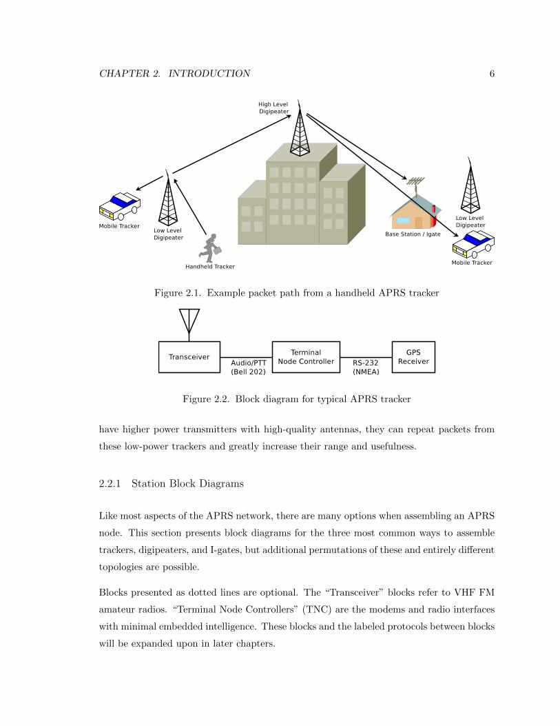
I-gates that receive the packet along the way. Figure 2.1 shows the typical path of a packet
from a low-powered handheld tracker as it moves throughout the local APRS network. It’s
not unusual for battery-powered trackers to only output one to five watts of RF power,
which limits their range to any stations immediately around them. Since digipeaters often
1The term tracker will be used in this paper to encompass all APRS nodes which move throughout thenetwork, not limited to those without receivers as the term is often used.
CHAPTER 2. INTRODUCTION 6
Figure 2.1. Example packet path from a handheld APRS tracker
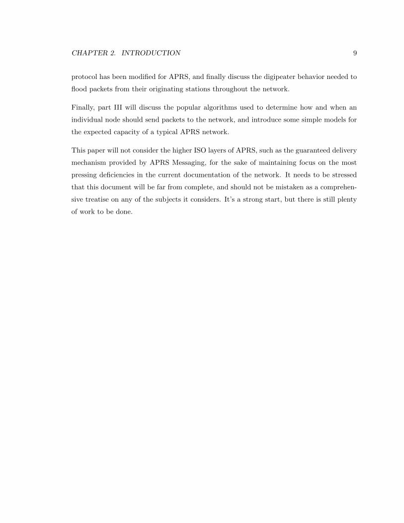
Figure 2.2. Block diagram for typical APRS tracker
have higher power transmitters with high-quality antennas, they can repeat packets from
these low-power trackers and greatly increase their range and usefulness.
2.2.1 Station Block Diagrams
Like most aspects of the APRS network, there are many options when assembling an APRS
node. This section presents block diagrams for the three most common ways to assemble
trackers, digipeaters, and I-gates, but additional permutations of these and entirely different
topologies are possible.
Blocks presented as dotted lines are optional. The “Transceiver” blocks refer to VHF FM
amateur radios. “Terminal Node Controllers” (TNC) are the modems and radio interfaces
with minimal embedded intelligence. These blocks and the labeled protocols between blocks
will be expanded upon in later chapters.

CHAPTER 2. INTRODUCTION 7
Figure 2.3. Block diagram for typical APRS Digipeater
Figure 2.4. Block diagram for typical APRS Internet Gateway
Figure 2.2 shows the block diagram for an APRS tracker, which is built around a Terminal
Node Controller which parses NEMA positions provided by a GPS receiver and converts
them into APRS position reports that are then frequency shift modulated and sent to a
VHF FM voice transceiver using an interface cable that includes transmit and receive audio,
as well as a line to key the “push to talk” button on the radio to start transmitting.
Figure 2.3 shows the block diagram for a digital repeater, which is similar to a tracker
except that the GPS receiver is often omitted. Since the digipeater is always installed in
a fixed location, its GPS coordinates can be hard-coded into non-volatile memory in the
TNC.
Figure 2.4 shows the block diagram for an Internet Gateway (I-gate), which like the digi-
peater doesn’t require a GPS receiver. Unlike the digipeater, instead of sending received
packets back out through the VHF transceiver, I-gates send received packets to the APRS-IS
Internet System via a local connection to the Internet.

CHAPTER 2. INTRODUCTION 8
Figure 2.5. The OSI network model as applied to APRS in this paper
2.3 Document Overview
The rest of this document is going to start at the bottom of the APRS protocol stack and
work its way up, touching on each layer with an introduction and some basic analysis.
Ideally, this document would answer all of the ambiguities existing in the APRS network
protocols, but many of the issues that will be touched upon deserve an entire masters thesis
of their own, and therefore will often be noted as simply deficient before moving on.
The rest of this document will be divided into three parts based on the bottom three layers
of the Open Systems Interconnection (OSI) model, to separately discuss issues found on
each of these layers of the APRS network stack. Figure 2.5 shows how the most popular
protocols used on APRS will be mapped to the OSI model, including the APRS messaging
system which will not be further mentioned due to it being a relatively unimportant part
of APRS.
Part I will cover the Bell 202 modem used to encode APRS on the VHF packet channels
and the KISS protocol used to connect modems to host devices such as computers. Chapter
3 will go into an unusual amount of detail since a specification document for Amateur Bell
202 was never written and therefore will likely prove to be one of the more significant
contributions of this paper to the field.
Part II will touch on what could be called the data link layer of APRS. It will start with
an introduction to the concept of a terminal node controller, move into how the AX.25
CHAPTER 2. INTRODUCTION 9
protocol has been modified for APRS, and finally discuss the digipeater behavior needed to
flood packets from their originating stations throughout the network.
Finally, part III will discuss the popular algorithms used to determine how and when an
individual node should send packets to the network, and introduce some simple models for
the expected capacity of a typical APRS network.
This paper will not consider the higher ISO layers of APRS, such as the guaranteed delivery
mechanism provided by APRS Messaging, for the sake of maintaining focus on the most
pressing deficiencies in the current documentation of the network. It needs to be stressed
that this document will be far from complete, and should not be mistaken as a comprehen-
sive treatise on any of the subjects it considers. It’s a strong start, but there is still plenty
of work to be done.

OSI Layer 1 — Physical
10
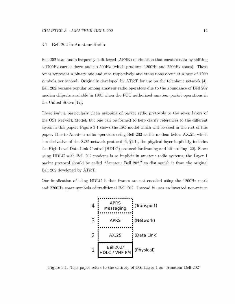
3 Amateur Bell 202
This chapter considers the most popular modulation used for APRS on RF, Amateur Bell
202. One of the major features of APRS is that large areas have standardized on single
VHF packet frequencies using this very-popular Amateur Bell 202 modulation. This is
what enables APRS tracker to move throughout the United States while beaconing on
144.390MHz and always be able to participate in the local APRS network. Surprisingly,
despite its age, this modulation still suffers from much confusion in its documentation, so
the primary points made in this chapter will be:
• Pointing out that what amateur radio operators call “Bell 202” implicitly extends
well beyond the original Bell 202 specification. Therefore, the new term “Amateur
Bell 202” is proposed to differentiate between the entire modem and the underlying
modulation.
• Drawing a new line between AX.25 and Amateur Bell 202 to make it clear that error
detection is a concern for the modem and not the data link protocol.
• Presenting a reference implementation of the checksum used to detect transmission
errors in Amateur Bell 202 frames.
• Discussing how the baseband modem signal should be modulated using VHF voice
radios and some challenges this presents to modem performance.
Despite Amateur Bell 202 as it is used in APRS often being decried for its age and vastly
outliving its usefulness, it can’t be denied that it is still an integral part of the amateur radio
digital communications landscape. While its deficiencies dictate that Amateur Bell 202 will
rarely be the best choice for new packet radio networks, its simplicity causes Amateur Bell
202 to be an appealing gateway into APRS and the digital communications hobby.
11
CHAPTER 3. AMATEUR BELL 202 12
3.1 Bell 202 in Amateur Radio
Bell 202 is an audio frequency shift keyed (AFSK) modulation that encodes data by shifting
a 1700Hz carrier down and up 500Hz (which produces 1200Hz and 2200Hz tones). These
tones represent a binary one and zero respectively and transitions occur at a rate of 1200
symbols per second. Originally developed by AT&T for use on the telephone network [4],
Bell 202 became popular among amateur radio operators due to the abundance of Bell 202
modem chipsets available in 1981 when the FCC authorized amateur packet operations in
the United States [17].
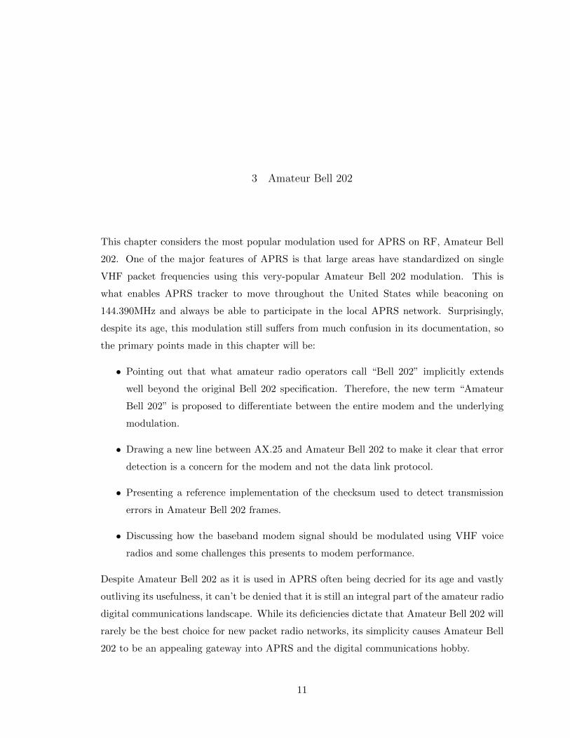
There isn’t a particularly clean mapping of packet radio protocols to the seven layers of
the OSI Network Model, but one can be formed to help clarify references to the different
layers in this paper. Figure 3.1 shows the ISO model which will be used in the rest of this
paper. Due to Amateur radio operators using Bell 202 as the modem below AX.25, which
is a derivative of the X.25 network protocol [6, §1.1], the physical layer implicitly includes
the High-Level Data Link Control (HDLC) protocol for framing and bit stuffing [22]. Since
using HDLC with Bell 202 modems is so implicit in amateur radio systems, the Layer 1
packet protocol should be called “Amateur Bell 202,” to distinguish it from the original
Bell 202 developed by AT&T.
One implication of using HDLC is that frames are not encoded using the 1200Hz mark
and 2200Hz space symbols of traditional Bell 202. Instead it uses an inverted non-return
Figure 3.1. This paper refers to the entirety of OSI Layer 1 as “Amateur Bell 202”

CHAPTER 3. AMATEUR BELL 202 13
1 2 3 4 5 6 7 8-0.8
-0.6
-0.4
-0.2
0
0.2
0.4
0.6
0.8
Symbol Period
Sig
na
l M
ag
nitu
de
Figure 3.2. Amateur Bell 202 signal representing the ASCII letter A (0x41)
Figure 3.3. Amateur Bell 202/HDLC frame format
to zero (NRZI) encoding, which calls for zeros in the original bit stream to be encoded
as a continuous-phase frequency transition between consecutive symbols, while ones are
encoded as the lack of a frequency change between two symbols [30]. Figure 3.2 shows a
typical Amateur Bell 202 signal representing the ASCII letter “A,” starting with the least
significant bit.
3.2 Amateur Bell 202 Transmission Format
Figure 3.3 shows the format of a typical single-frame Amateur Bell 202 transmission, as it
is based on HDLC. There are a number of important facets to note:
• The leading 0x00 octets are mentioned in very few documents discussing Amateur

CHAPTER 3. AMATEUR BELL 202 14
Bell 202, yet they reportedly improve modem throughput [21][29]. 0x00 encoded in
NRZI causes a symbol transition every clock cycle and thus provides a more effective
clock synchronization target than the originally specified 0x7E octets. 0x7E is actually
the longest allowable string of 1s in the frame and therefore has the lowest amount of
energy at the clocking frequency, which causes it to be the worst octet for asynchronous
clock recovery.
• The octet 0x7E is used to indicate the beginning and end of HDLC frames. There is
little guidance on the number of flag octets needed before or after frames in Amateur
Bell 202 (represented by N2 and N3 in Figure 3.3) beyond stating that there must be
at least one of each.
• The sum of N1 and N2 is variable in most modems via the “TXDelay” parameter,
which specifies how long the preamble should be, in 10ms increments.
• It is permissible to encode multiple frames per transmission, yet there is no guidance
as to how many octets of 0x7E should be included between them; most modems in-
sert several 0x7E octets between frames.1 Tests indicate that many demodulators are
sensitive to the number of flags before, between, and after frames as mentioned in
the last three points. Finding definitive minimums would require testing a represen-
tative sample of the popular Amateur Bell 202 modems, which is beyond the author’s
resources.
• The frame payload and frame checksum must be modified such that no string of more
than five 1’s happen to appear in a row. This is done by “bit-stuffing” the transmitted
bitstream by appending a zero after any string of five ones at the transmitter, and
subsequently dropping this zero following five ones at the receiver.2
• Every octet is encoded and transmitted least-significant bit first, except for the CRC-
16-CCITT frame checksum, which is transmitted big-endian and most-significant bit
first. [6, §3.8], [16, §8.1.1-2], [22]. See Section 3.2.2 for further discussion.
1For a specific example, the Argent Data OT3m TNC with firmware r56474 inserts 3 flags before a frame,7 flags between two frames, and 5 flags after the final frame.
2Six ones in a row represent a 0x7E flag indicating the end of a frame or an idle carrier. Seven or moreones in a row indicate an invalid channel state that shouldn’t happen, but regularly does, so modems mustbe able to handle arbitrary strings of ones gracefully.
CHAPTER 3. AMATEUR BELL 202 15
• The minimum and maximum payload sizes indicated in Figure 3.3 aren’t enforced
by any properties of Bell 202 or HDLC, but from the Maximum Transmission Unit
(MTU) specified in the Layer 2 AX.25 network protocol. Larger frames are possible
and were often used in specialized AX.25 and IPv4 packet networks [24]. A practical
upper limit on frame size is enforced by the need for successful frames to be completely
error-free.
3.2.1 Excluding HDLC from Layer 2 AX.25
It is important to note that the presentation of the HDLC framing and checksum in Figure
3.3 as part of the Layer 1 modulation instead of as part of the Layer 2 AX.25 frame is novel
to this work and hasn’t been seen in any of the existing literature. This classification isn’t
consistent with the traditional OSI model, but the author’s main objective is to decouple
HDLC from AX.25. This change is suggested because including the frame checksum and
flags in the Layer 2 documentation confuses the separation between Amateur Bell 202 and
AX.25, which should be independent protocols.
This is particularly important when AX.25 packets are transported across other Layer 1
links which use their own framing protocols. The Keep It Simple Stupid (KISS) serial
link between a host system and modem is the most notable transport where the HDLC
fields are not included in outgoing frames, and are instead post-facto generated by the
modem during transmission3 [12]. M. Chepponis and P. Karn made the technically correct
decision of excluding HDLC framing from the AX.25 payload when developing KISS, but
this causes an unfortunate situation where KISS is transporting an entirely undocumented
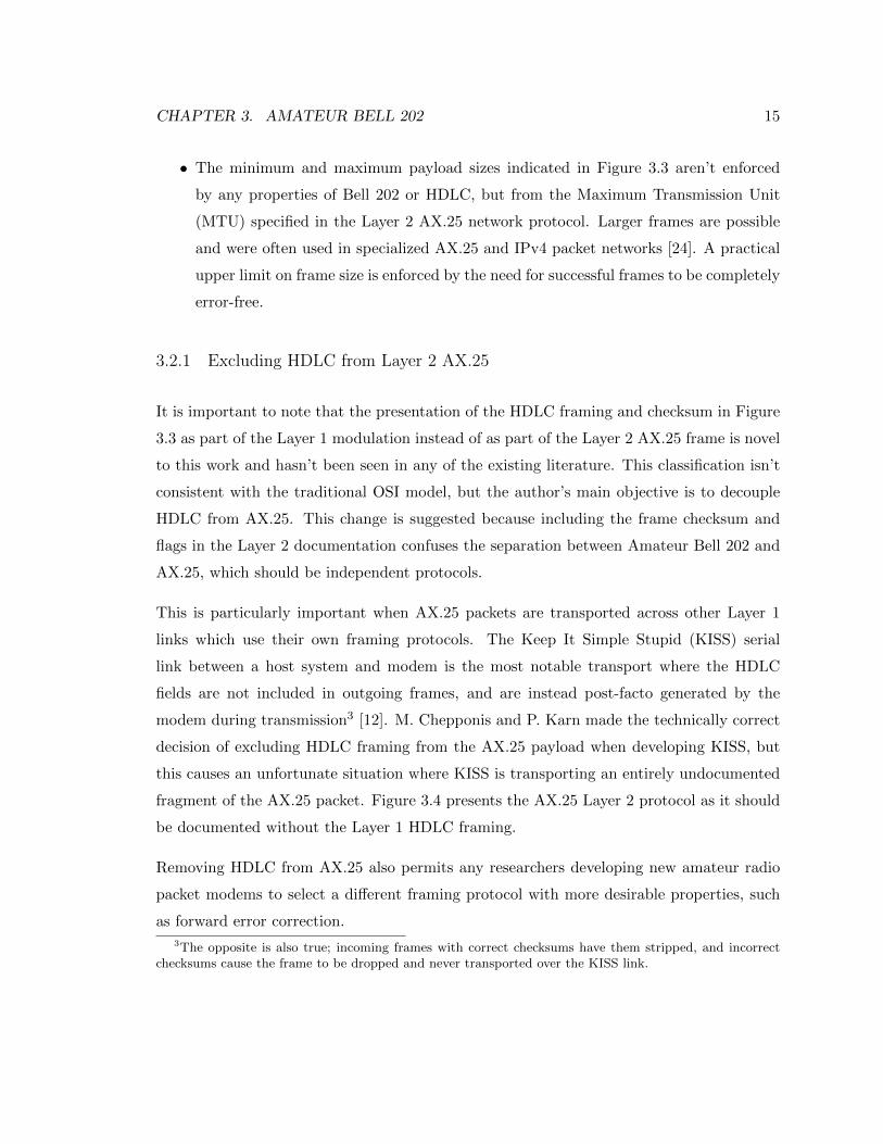
fragment of the AX.25 packet. Figure 3.4 presents the AX.25 Layer 2 protocol as it should
be documented without the Layer 1 HDLC framing.
Removing HDLC from AX.25 also permits any researchers developing new amateur radio
packet modems to select a different framing protocol with more desirable properties, such
as forward error correction.
3The opposite is also true; incoming frames with correct checksums have them stripped, and incorrectchecksums cause the frame to be dropped and never transported over the KISS link.

CHAPTER 3. AMATEUR BELL 202 16
Figure 3.4. Modified AX.25 packet format excluding HDLC fields.
1: function calculate crc(frame[ ], frame length)
2: crc← 0xFFFF
3: for all byte← frame0, frameframe length−1 do
4: for all bit← byteLSb, byteMSb do
5: if crcLSb 6= bit then
6: crc← (crc� 1) XOR 0x8408
7: else
8: crc← crc� 1
9: end if
10: end for
11: end for
12: crc← crc XOR 0xFFFF
13: return crc
14: end function
Figure 3.5. Algorithm to calculate CRC-16-CCITT in reverse-bit order.
3.2.2 Calculating the Frame Check Sum
The Frame Check Sum (FCS) used for error detection in Amateur Bell 202 is the well-known
CRC-16-CCITT, which enjoys a wide deployment in network protocols and systems.4 Un-
fortunately, the language used in §4.2.5 of the ISO specification for HDLC [30] is particularly
awkward, and does not lend itself well to implementation. For the sake of clarity, Figure
3.5 presents one possible algorithm to calculate the FCS of a complete frame, which is im-
plemented in ANSI C in Appendix A. The constant 0x8408 comes from a bit reversal of
the 0x1021 generator polynomial since the presented algorithm calculates the CRC in bit
4Example systems using CRC-16-CCITT include HDLC, Bluetooth, the XMODEM file transfer protocol,and SD cards.
CHAPTER 3. AMATEUR BELL 202 17
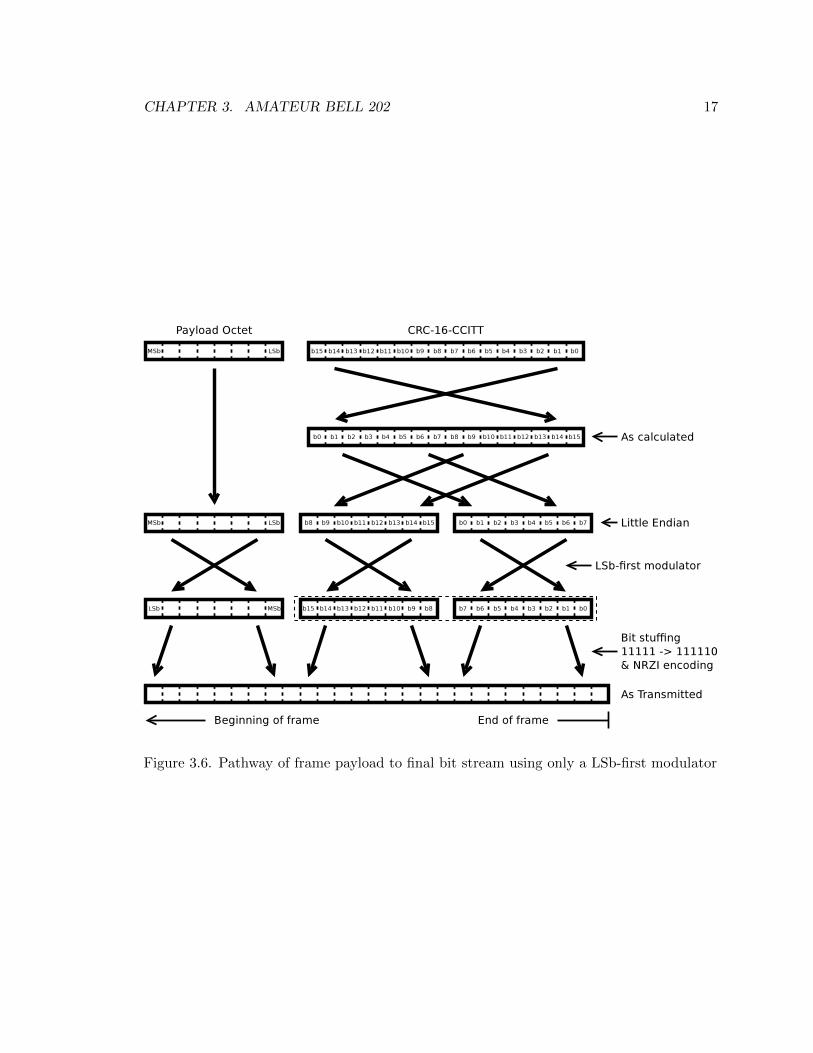
Figure 3.6. Pathway of frame payload to final bit stream using only a LSb-first modulator
CHAPTER 3. AMATEUR BELL 202 18
reversed order.
The order of the two octets and bit order of the checksum as transmitted over the air is
particularly muddled in the existing amateur radio literature. Many sources call for sending
the checksum little-endian, while ITU V.42 §8.1.2.3 clearly specifies big-endian, as is the
convention for most network protocols. The original specifications also call for transmitting
the checksum most significant bit (MSb) first, which is the opposite of the payload octets.
This exception is noted in §3.8 of the AX.25 specification as well.
This creates plenty of confusion on the part of implementers, which is likely caused by the
fact that available reference implementations of the CCITT checksum don’t make it clear
that they already integrate the needed bit reversal after the Cyclic Redundancy Check
(CRC) division and one’s complement. The algorithm presented in Figure 3.5 does not
calculate the true CCITT CRC, but follows the convention of calculating it in reverse-bit
order, such that the final bit-reversal step may be omitted during modulation of the bit
stream while using the least significant bit (LSb) first modulation subroutines already used
for the payload data. Therefore, the checksum as presented should be sent lower octet first,
using the same modulator as for payload octets that modulates the LSb-first. This ensures
that the resulting checksum as transmitted will have the correct sequence, starting with the
MSb and finishing with the LSb, and is why many implementations appear to completely
ignore the need to send the FCS MSb. Figure 3.6 demonstrates how calculating the FCS in
reverse bit order and then feeding it through the same LSb-first modulator as the payload
octets is equivalent to calculating the FCS in canonical bit order and using a separate MSb-
first modulator. This is desirable because it prevents the need for this second subroutine to
send bits MSb-first to ever be written or maintained.
3.3 FM Deviation and Emphasis
Once the Amateur Bell 202 frame is generated, encoded using NRZI, and converted into a
baseband AFSK signal, it still needs to be converted into a VHF FM signal and transmitted
to other stations. Since Bell 202 was originally designed for telephone data service, the
existing specifications give no guidance on the unique aspects of the amateur VHF FM
physical layer. One such issue is what value of FM deviation to target when setting modem
CHAPTER 3. AMATEUR BELL 202 19
audio levels.
While quantitatively justifying this value is beyond the ability of the author, a proposed
specification for FM deviation is 3.5kHz for both the 1200Hz and 2200Hz tones, or for the
wider of the two tones if equal deviation is not possible [21].
This proposal is complicated by two major issues:
• The lack of availability of the necessary test equipment to measure FM deviation.
• The inconsistency in pre-emphasis and de-emphasis filters used by individual network
nodes.
The VHF deviation meter needed to properly set modem deviation is prohibitively expensive
for the typical packet radio operator, so presenting a figure such as 3.5kHz deviation to most
users does little good. Qualitative and home-brew solutions have been developed for setting
deviation levels [2], and these techniques should be better promoted until deviation meters
become a more standard part of a packet operator’s toolkit.
Pre-emphasis and de-emphasis is a concept in FM voice communications where higher
baseband frequencies are modulated with larger deviation than lower frequencies to provide
a consistent signal-to-noise ratio across the channel. Unfortunately, the advantages of these
audio filters to packet operation are debatable, and they are not applied consistently. A
single packet station is likely to have any permutation of pre-emphasized or flat transmit
audio and de-emphasized or flat receive audio. This means that even when one station
deliberately uses flat audio, there is no guarantee that it won’t suffer from receiving another
station’s pre-emphasized signal or be received by another station using de-emphasis.
Different types of Bell 202 modems vary in how sensitive they are to this high/low pass
filtering effect More importantly, there is no specification established for what level of pre-
/de-emphasis a modem should tolerate. One suitable source for such a benchmark would be
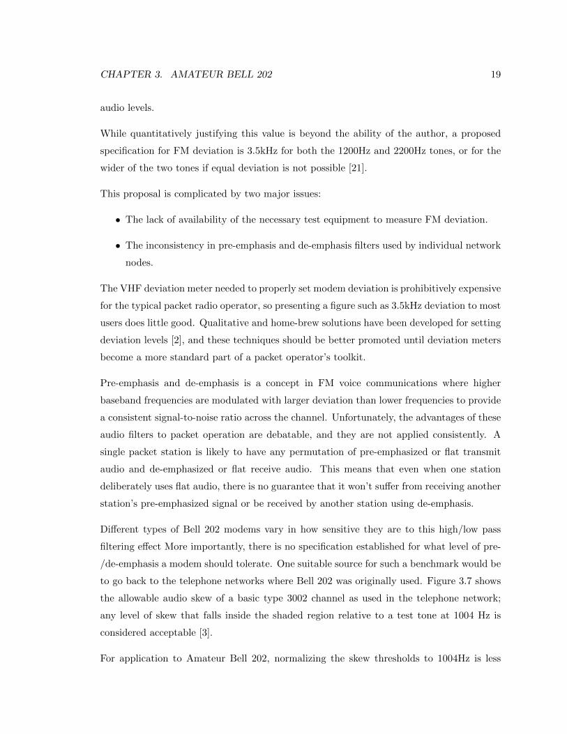
to go back to the telephone networks where Bell 202 was originally used. Figure 3.7 shows
the allowable audio skew of a basic type 3002 channel as used in the telephone network;
any level of skew that falls inside the shaded region relative to a test tone at 1004 Hz is
considered acceptable [3].
For application to Amateur Bell 202, normalizing the skew thresholds to 1004Hz is less
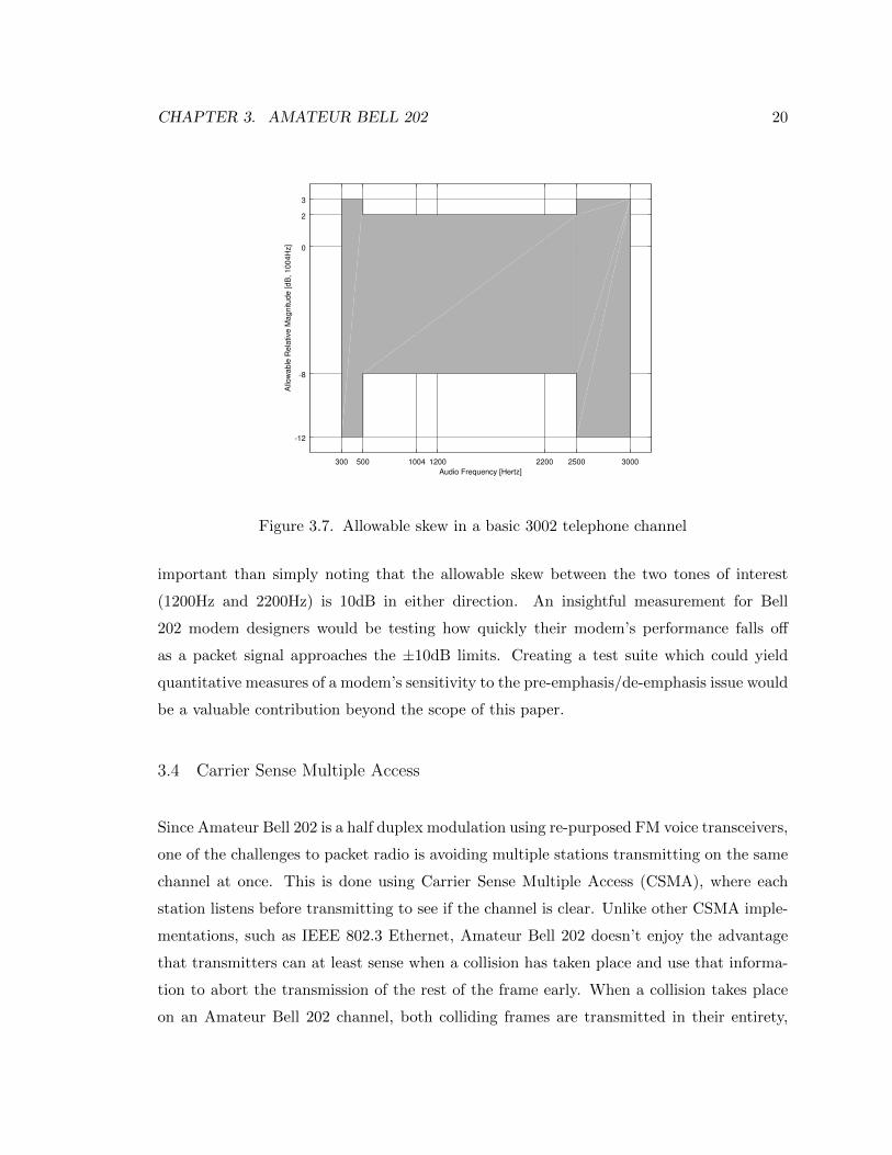
CHAPTER 3. AMATEUR BELL 202 20
300 500 1004 1200 2200 2500 3000
-12
-8
0
2
3
Audio Frequency [Hertz]
Allo
wa
ble
Re
lative
Ma
gn
itud
e [
dB
, 1
004
Hz]
Figure 3.7. Allowable skew in a basic 3002 telephone channel
important than simply noting that the allowable skew between the two tones of interest
(1200Hz and 2200Hz) is 10dB in either direction. An insightful measurement for Bell
202 modem designers would be testing how quickly their modem’s performance falls off
as a packet signal approaches the ±10dB limits. Creating a test suite which could yield
quantitative measures of a modem’s sensitivity to the pre-emphasis/de-emphasis issue would
be a valuable contribution beyond the scope of this paper.
3.4 Carrier Sense Multiple Access
Since Amateur Bell 202 is a half duplex modulation using re-purposed FM voice transceivers,
one of the challenges to packet radio is avoiding multiple stations transmitting on the same
channel at once. This is done using Carrier Sense Multiple Access (CSMA), where each
station listens before transmitting to see if the channel is clear. Unlike other CSMA imple-
mentations, such as IEEE 802.3 Ethernet, Amateur Bell 202 doesn’t enjoy the advantage
that transmitters can at least sense when a collision has taken place and use that informa-
tion to abort the transmission of the rest of the frame early. When a collision takes place
on an Amateur Bell 202 channel, both colliding frames are transmitted in their entirety,
CHAPTER 3. AMATEUR BELL 202 21
but both are lost and the channel time wasted.
Besides the degenerate case of ignoring the current channel status completely when deciding
to transmit a pending frame,5 there are two popular algorithms used for channel access in
North America; DWait and P-persistent.
DWait is a deterministic algorithm where each station is assigned a fixed “quiet time” after
the end of any other transmission before they will begin a locally pending transmission.
This lends itself well to designed networks where the relative priority of each station is
known and a corresponding DWait time is set for each station where a shorter DWait will
always gain the channel over a longer one. Conversely, this doesn’t lend itself well to ad-hoc
networks, since two stations that happen to both operate near one another with similar
DWait parameters will tend to collide and reduce throughput.
P-persistent is a stochastic algorithm that attempts to randomly spread stations apart when
the channel becomes clear. This is configured with two variables: the slot time (SLottime),
and the probability that a station should choose to transmit during a given slot (PErsist).
The SLottime should be set to as short of a time interval as possible during which a station
can reliably identify another station as transmitting before beginning its own transmission.
The PErsist value should be tuned based on how likely another station is to transmit during
the same time slot considering the number of other stations with pending traffic attempting
to gain the channel.
A typical modem supporting the P-persistent algorithm will need three values adjusted
based on the specific network hardware in use; PErsist, SLottime, and the transmitter
preamble time TXDelay mentioned earlier in this paper.
• PErsist: Measured in units of 1/256, the suggested default is 63, which translates
into a 0.25 chance of selecting a specific available slot [12]. A typical implementation
selects a random number in the range [0,255] and tests if it is equal or less than the
PErsist value. Therefore, a setting of 0 would result in a 0.004 chance of selecting a
slot and a setting of 255 would result in always selecting an open slot. The optimal
value for a specific network is highly dependent on the local channel occupancy, so
5This is a surprisingly common channel access method, used primarily by what are called “dumb” or“deaf” APRS trackers, which are transmit-only and lack an FM receiver altogether.

CHAPTER 3. AMATEUR BELL 202 22
the suggested default shouldn’t be considered definitive.
• SLottime: Measured in units of 10ms increments, the traditional default from sources
such as the KISS specification and Kantronics hardware is a value of 10 (100ms)
[12][18], but performance measurements of contemporary VHF radios indicate a need
for a longer slot time. The new suggested value is 30 (300ms), which is discussed
further in Appendix B.
• TXDelay: Measured in units of 10ms increments, the suggested default is a value of
50, which translates into a 500ms synchronization preamble from when a transmitter
is keyed up until when a payload frame is transmitted [12]. This value is very con-
servative and can usually be reduced when receiving stations are properly configured
with well aligned clock recovery mechanisms.
There are additional channel access methods beyond the two mentioned above that are
applied in amateur radio packet networks. Examples include Demand Assigned Multiple
Access (DAMA), which is primarily used in European packet networks, and Time Slotting,
which is used in carefully designed high-throughput networks. Since these alternatives see
less application in American packet networks, they are excluded from this discussion and
the reader need only appreciate that this is not a comprehensive survey of channel access
methods.
3.5 Conclusion
By most measures, Amateur Bell 202 is a very poor performing modulation to be used by
amateurs for packet operations. One-bit symbols cause Bell 202 to suffer from poor spectral
efficiency, HDLC lacks any error correcting codes so single-bit errors cause entire frames to
be dropped, and 1200 bits per second is a remarkably low data rate when even consumer
radio systems are operating at hundreds of millions of bits per second throughput.
One aspect of Amateur Bell 202 that is appealing, other than the huge legacy systems still
using it, is its relative simplicity. The fact that amateurs are able to implement Amateur
Bell 202 modems on systems as minimalistic as 8 bit microcontrollers, and that modems
can interface with unmodified voice radios, make it possible for amateur radio operators to
CHAPTER 3. AMATEUR BELL 202 23
build their own APRS nodes with relatively little difficulty.
Faster data rates and more sophisticated modems aren’t being discouraged, but the value
of being able to learn about amateur digital communications via the simplicity of Bell
202 shouldn’t be discounted. The public APRS networking is deeply entrenched in using
Amateur Bell 202, so exploring future enhancements to the Amateur Bell 202 modem is a
topic that begs for further examination.
4 KISS
During the early 1980’s when amateur Terminal Node Controllers were developed, the
expectation was that the TNC would be handling the entire packet protocol stack up to the
final presentation to the user. This would have been done using a dumb terminal, such as
a VT100, or line printer and a keyboard. As personal computers became affordable in the
late 1980’s, the expectation that the entire application stack would run on the embedded
TNC became severely limiting and KISS (“Keep It Simple, Stupid”) emerged as the solution
to expose the modem inside TNCs via an eight bit clean interface and bypass the TNC’s
internal network stack.
KISS was originally presented by Mike Chepponis, K3MC and Phil Karn, KA9Q at the 6th
ARRL Computer Networking Conference in Redondo Beach, CA [12]. KISS was designed
as an extension to the Serial Line Internet Protocol (SLIP) allowing for in-band signaling
from the host to the TNC to enable setting modem configuration parameters such as the
preamble length and CSMA parameters.
This meant that the existing TNCs with their radio interfaces could be upgraded once
with new ROMs that supported KISS and any new network behavior or protocol could
be implemented on a separate host PC. This was particularly valuable since personal PCs
were much more productive development environments than the 256kb EPROMs and 8 bit
Z80 microprocessors of the popular Tucson Amateur Packet Radio TNC 2 product and its
clones [32].
24
CHAPTER 4. KISS 25
4.1 Isolating Modulation from Network
The advantage of KISS is that it has become the standard packet interchange protocol
between TNC modems and host network controllers, enabling each side to experiment with
new protocols. This means that as the APRS protocol has evolved, stations that used the
KISS protocol are able to continue using the same ROM-based modems and only need to
upgrade the software running on their host system. This abstraction holds up even further
in that it allows operators to use different data link protocols than AX.25, yet there have
been few examples of this since the collapse of the IPv4 amateur radio networks with the
wide-spread deployment of the Internet.
As discussed in the prior chapter, as Bell 202 and HDLC begin to show their age, the
field is ripe for a new modulation to replace them on VHF/UHF packet networks. Should a
researcher wish to deploy a new modulation to use under APRS, all that needs to be done is
build new KISS modems, which will seamlessly interface with most existing APRS software.
Replacing Amateur Bell 202 modems has always been a popular subject of discussion on
the APRS mailing lists, and is an area ripe for future quantitative study.
4.2 Shortcomings of KISS
While originally presented as an interim solution until a better protocol was developed, KISS
has enjoyed a lasting popularity among its users. One concern about KISS that has spawned
several derivative protocols is the lack of a checksum used in each KISS frame. Should any
bit errors happen between the host system and the modem, they may go undetected and
cause corruption in the transported payload as it continues through the network. One of the
most popular of these derivatives of KISS is SMACK (Stuttgart Modified Amateurradio-
CRC-KISS), which is a backwards compatible extension to KISS which includes a frame
checksum to protect against frame corruption [28].
Traditionally, KISS links between the host PC and KISS modems have been deployed over
relatively short RS-232 serial links (three to six feet). An increasing number of contemporary
modems are moving to a pure USB implementation. What the author has been unable to
find is any evidence that, when correctly deployed, these types of short serial links have

CHAPTER 4. KISS 26
any risk of corruption which is avoided by using the SMACK extension. Further study is
needed to examine typical APRS KISS deployments to justify the additional effort required
to implement and deploy SMACK above KISS to protect against any possible corruption
risks.
A second shortcoming of KISS which has not evoked anywhere near the level of discussion
that the corruption issue has is KISS’ lack of any way for modems to pass out-of-band
(OOB) information back to the host PC. KISS defines numbered command codes for the
host to pass information to the modem, including channel access settings and hardware
specific settings beyond the type ‘0’ data frame that should be transmitted on the channel.
In the opposite direction, from modem to host, the KISS specification explicitly limits frame
types to only data frames. This disallows hosts from being able to interrogate modems as
to their current configuration settings or any information about the RF channel beyond
packets as they are received.
The author suggests that a revision to the KISS specification be considered that would
allow modems to pass non-zero payloads back to the host PC. Legacy applications would
need to properly discard these non-zero frames as OOB data that they are not interested in,
while enabling new applications such as interactive configuration programs and give more
meaningful metrics as to current channel utilization.
• An interactive configuration program would allow a user to request a dump of the
current configuration, edit it, and re-upload it to one or several KISS modems. A
canonical example of this type of application is the OTWINCFG tool provided by
Argent Data for their trackers [5, §17.6].
• Channel utilization information could include how much time is consumed on the chan-
nel by AFSK data that does not decode as valid packets. Some APRS applications
attempt to estimate channel utilization based on received packets, which will con-
sistently under-estimate the actual figure due to frame preambles and frames which
fail their checksums never being reported. The worst case of continuous collisions
would result in the application misinterpreting no received packets as an entirely idle
channel, where the opposite is the actual case.
CHAPTER 4. KISS 27
4.3 Conclusion
KISS have proven itself tremendously useful as it has decoupled the modem hardware from
the network protocol used above it. The decreasing price and size of single-board computers
such as the Texas Instrument’s BeagleBone have cemented the popularity of network nodes
built using a full-fledged computer that uses a KISS modem as a radio interface. It should
be appreciated that KISS enables the development of new modulation schemes without the
need to modify existing APRS software to run over new higher-quality links. Future work
involving KISS should include studying the quantitative risks of not using checksums on
the serial link between the host and the modem and the feasibility of extending KISS to
allow OOB information to be passed from modem to host.

OSI Layer 2 — Data Link
28
5 AX.25
AX.25 is the amateur radio derivative of CCITT X.25 that was designed during the early
1980’s as the primary data link protocol used by amateur packet networks. The AX.25 spec-
ification has been maintained by the Tucson Amateur Packet Radio (TAPR) organization
until its latest release, Version 2.2 in July of 1998.
The most significant difference between AX.25 and the original X.25 protocol lies in the
hardware addresses used by AX.25, which are based on the expectation of each station using
their FCC-issued callsign. Each node is addressed by their callsign plus an additional 4 bit
secondary station identifier (SSID), which allows each licensee to maintain and operate up
to 16 stations in each packet namespace.
AX.25 is one of the best-documented protocols used in amateur radio packet networks, so
it could be argued that a chapter in this thesis considering AX.25 could be omitted. The
AX.25 specification goes into tremendous detail as to the expected behavior of each node
and how the system should transition between states. Where documentation does fall short
is in how APRS abuses a small subset of the AX.25 protocol for the specific needs of the
APRS network. The rest of the chapter will walk through each field of the AX.25 packet
and note how it is used by APRS, followed by a discussion of the implications of the FCC
requirement to identify an active transmitter by its FCC-issued license every ten minutes.
5.1 Header Format for APRS
A very limited subset of the complete AX.25 protocol is used by APRS due to APRS
deliberately avoiding the use of any of the connected or control modes of AX.25. This means
that any AX.25 protocol stack used for APRS need only support Unnumbered Information
29
CHAPTER 5. AX.25 30
Figure 5.1. AX.25 UI Packet Format
(UI) frames, and many APRS protocol stacks cannot handle any other forms of AX.25
traffic. Figure 5.1 presents the modified form of the AX.25 frame that is used by APRS.
5.1.1 TNC Description / Destination Address
Traditional AX.25 traffic is usually directed at a single station, which would be indicated
by a packet’s destination address. Since APRS is strictly a one-to-many network protocol
at Layer 3, this field was deemed not needed for APRS and several alternative uses for the
field have been proposed.
The most popular application for this field is to be used as a tracker identifier, where a six
character identifier is allocated from the APRS Working Group to identify a specific APRS
TNC and firmware version. This provides valuable information to the rest of the APRS
network. APRS TNCs often “misbehave” and it is helpful to be able to immediately identify
the original developer for a remote APRS node. Experimental trackers which have not yet
received a tracker ID may use the APZ prefix with three additional arbitrary alphanumeric
characters as their TNC identifier.
5.1.2 Source Address
The source address is either the FCC-issued or a “tactical” callsign used by the beaconing
APRS station, with an additional SSID appended to the station, which may range from
zero to 15. Source addresses must be at least three characters long, and may not be any
longer than six. Stations using AX.25 over RF are limited to the SSID’s of 0 to 15 due to
AX.25’s binary format, while APRS imposes a looser standard such that the SSID is only
limited to two alphanumeric characters when not transported over AX.25 links..

CHAPTER 5. AX.25 31
5.1.3 Routing Path
The AX.25 routing path is an optional variable-length field consisting of an ordered list of
digipeaters which should process and re-transmit the considered packet. Should a station
not require the use of this field, it can be completely omitted and the end-of-path bit should
be set on the source address field. The path must consist of an integer number of seven
octets.
The original AX.25 version 2.0 spec allowed for anywhere from zero to eight digipeaters to
be included in an AX.25 frame. Unfortunately, due to the unreliable nature of amateur
packet radio, packets with a routing path requesting as many as eight hops would rarely
be successfully delivered to the end station. The version 2.2 specification for AX.25 was
rewritten limiting the number of requested digipeaters to two with the argument that pack-
ets traveling beyond two hops should be handled by a higher layer protocol than AX.25.
Because AX.25 doesn’t guarantee delivery from a digipeater to another station, packets
passing through a digipeater that are lost need to be resent from their origin. Higher
layer protocols can recover from a lost packet locally without needing to twice consume the
bandwidth used to get the packet to the digipeater.
This concept of higher-layer retries and a limit of two digipeaters introduced in AX.25 v2.2
is ignored by APRS. More than two digipeaters are often seen on APRS traffic, and users
are only strongly discouraged from using a large number of hops.
5.1.4 Control Flags
The Control Flag octet indicates different modes for the AX.25 frame. Since APRS strictly
uses only Unnumbered Information (UI) frames, this field must contain the value 0x03.
5.1.5 Protocol IDentifier
The Protocol IDentifier (PID) field is normally used to identify the Layer 3 protocol being
transported by AX.25. TAPR has reportedly stopped processing requests for new PID
values to be issued to new Layer 3 applications of AX.25 [20], which is a possible explanation
CHAPTER 5. AX.25 32
for why APRS doesn’t have a unique PID. It instead uses the value of 0xF0, incorrectly
indicating that no Layer 3 protocol is in use.
5.1.6 Information Field
The rest of the AX.25 frame contains the APRS payload in what is called the Information
Field. The end of the Information Field is indicated by the Layer 1 modulation, which is
traditionally the Amateur Bell 202 FCS and 0x7E flag.
The maximum transmission unit for the Information Field is 256 octets, and APRS imposes
a minimum of one octet identifying the type of APRS packet being carried [33].
5.2 FCC Identification Requirements
One of the conditions of operating a radio under FCC Title 47 CFR Part 97 is that amateur
radio operators are required to transmit their callsign at least once every ten minutes during
an exchange. An ongoing source of controversy in the APRS community is what this means
for operating an APRS node, and particularly digipeaters.
The source of argument is what constitutes properly identifying the transmitting station;
only a station’s FCC callsign in the source address field, or simply including the callsign
somewhere in the complete frame. Considering only the source address field as a valid
way to identify a station is a very conservative interpretation of §97.119, but establishes
the requirement that every digipeater active in the APRS network needs to originate a
new packet every ten minutes. Alternatively, accepting the digipeater’s callsign injected
anywhere in an outgoing packet lends itself to the digipeater staying more “quiet” since
appending its callsign to the end of the routing path of incoming packets could be considered
identification enough.
The considered disadvantage of the more conservative interpretation is that the additional
beacons being generated by every active digipeater every ten minutes is an excessive burden
on the APRS network. Digipeaters rarely have information of value to the rest of the
APRS network, so their beacons are seen as little more than noise. This interpretation also
prohibits the use of “tactical” callsigns, which are selected to convey more useful information

CHAPTER 5. AX.25 33
that the control operator’s callsign. One common example is digipeaters on major mountain
peaks; a digipeater on Tassajara peak beaconing as “TASS” has a more meaningful name
than beaconing as its owner’s FCC callsign. The FCC callsign is then placed somewhere in
the comment section of the APRS beacon.
The issue with identifying via appending callsigns to other station’s packets and using
tactical callsigns is that it isn’t always clear what a station’s callsign is.
• Many digipeaters fail to correctly append their callsign to routing paths when they
process packets, so the last callsign in the path isn’t necessarily the station transmit-
ting it.
• There is no standard secondary place for a station’s “real” callsign when using a
tactical call. Operators often program digipeaters with comments that fail to make it
clear what their callsign actually is.
In the end, the question of how each station needs to identify to meet part 97 is a strictly
legal one. Arguments have been made for interpreting §97.119 several places between these
two extremes, and the final decision on how to interpret the legal requirements are left up
to the individual amateur radio operators and the federal government’s lawyers.

6 Digital Repeater Routing Behavior
When the AX.25 networks were originally built in the 1980s, one of the fundamental design
assumptions was that every node was physically static in the network. Digipeaters were
installed on top of high buildings or mountain tops, and client nodes were modems connected
to bulky video terminals or desktop PCs. When two stations wanted to exchange packets,
the operators had to manually construct an explicit list of digipeaters to use to deliver
packets to the other station. Should a station move to a new area, the operator would need
to discover new near-by digipeaters and manually construct routing paths using them.
One of the design goals of APRS has been to support mobile nodes, so this requirement to
pre-facto be aware of the local infrastructure is unacceptable. The solution was to categorize
digipeaters into a small number of “aliases” such that a digipeater would respond to both its
specific callsign and to any of its aliases. A mobile station expecting to move throughout the
APRS network could then construct its routing paths purely out of digipeater aliases and
use the network infrastructure despite not knowing each digipeater’s callsign or location.
As APRS has grown from an experimental network to one that covers much of the country,
it has adopted and discarded multiple sets of digipeater aliases. As the expectations as to
each node’s behavior regarding those aliases have changed, the APRS community has failed
to make it clear that the previous behavior has been deprecated. The rest of this chapter
will walk through the history of the basic set of routing aliases, followed by an overview of
possible digipeater behaviors.
More than anything else, this chapter is going to highlight how ambiguous the APRS
specification is in regards to digipeater behavior. Most of the aliases discussed in the
original APRS protocol specification have been subsequently deprecated, without the APRS
specification being amended to indicate as such. The APRS specification also failed to have
34

CHAPTER 6. DIGITAL REPEATER ROUTING BEHAVIOR 35
a detailed discussion on digipeater behavior, so many different interpretations and ideas have
been developed, which has created several divergent schools of thought on what behavior
is best. Writing a definitive analysis on digipeater behavior is a large undertaking that
warrants further consideration beyond what is possible in this work.
6.1 Routing Aliases
The original definition of APRS included several aliases, the most notable of which were
RELAY and WIDE. Digipeaters were divided into two categories depending on if they were
high-level (on the top of large towers, mountain tops, etc.) or low-level (typically residential
sites). Low-level sites would only digipeat packets which used the RELAY alias or the
digipeater’s literal callsign, where high-level digipeaters would respond to both RELAY and
WIDE in addition to their callsign. This enabled a user to selectively include or exclude
the numerous low-level digipeaters depending on if the station had sufficient power to reach
the high-level WIDE digipeaters or needed the low-level receivers to assist with being heard
on the network.
A station would construct their desired routing path as an ordered list of callsigns and
aliases. For example, a station requesting three high-level hops out from their position
would use the routing path “WIDE,WIDE,WIDE” when beaconing in a new area where
the local digipeater callsigns were unknown. Since these strings of several WIDE aliases
proved to be common, the APRS community developed the concept of WIDEn-N, where
multiple WIDE aliases are summarized as a single routing alias to reduce the average packet
length on the network.
A WIDEn-N alias represents multiple WIDE aliases by using two numbers, represented by
n and N. The first n represents the originally requested number of WIDE hops, where the
trailing N represents the remaining number of hops that have not yet been consumed.
Therefore, the alias “WIDE3-2” represents an original request for three hops that has
already been processed by one digipeater. Once a WIDEn-N alias gets decremented to
WIDEn-0, it is considered entirely consumed, having been processed by n digipeaters.
Low-level “fill-in” digipeaters are needed to assist low-power moving trackers in reaching the
primary high-level digipeater network before it is possible to be received by other stations.
CHAPTER 6. DIGITAL REPEATER ROUTING BEHAVIOR 36
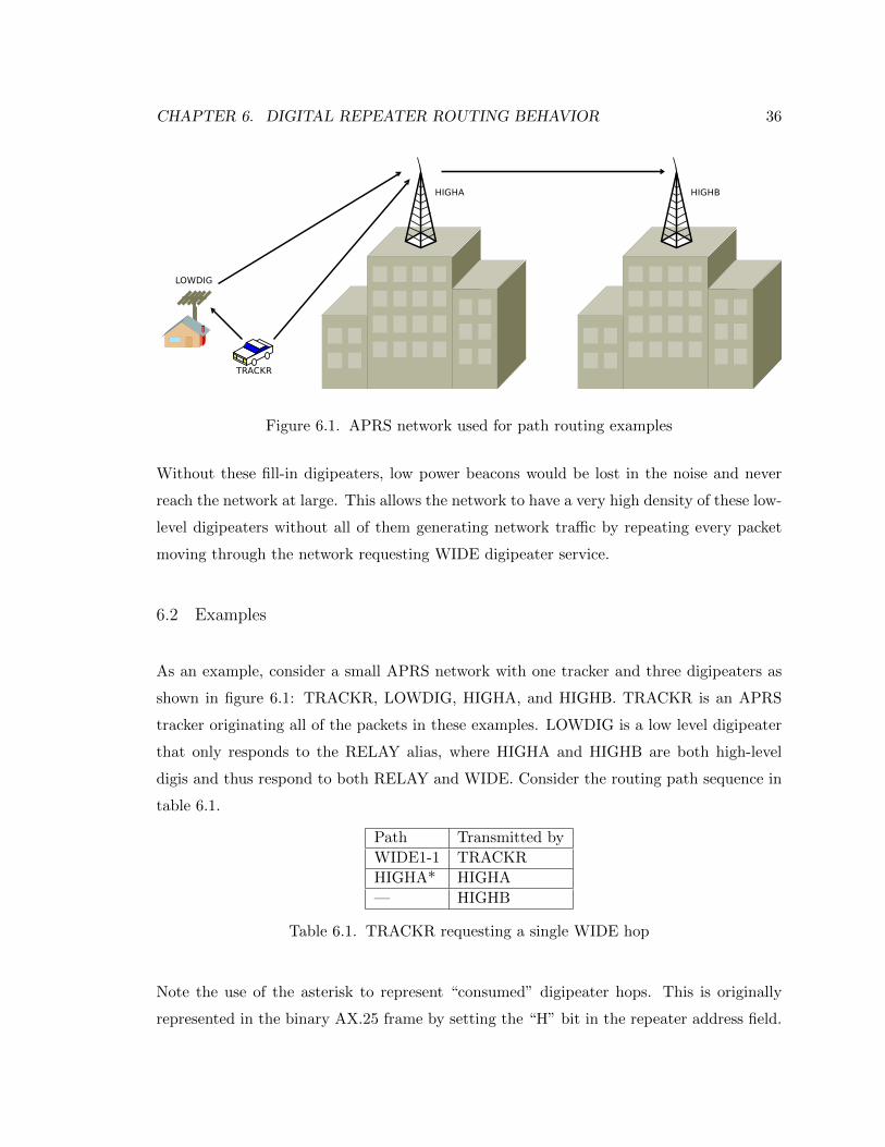
Figure 6.1. APRS network used for path routing examples
Without these fill-in digipeaters, low power beacons would be lost in the noise and never
reach the network at large. This allows the network to have a very high density of these low-
level digipeaters without all of them generating network traffic by repeating every packet
moving through the network requesting WIDE digipeater service.
6.2 Examples
As an example, consider a small APRS network with one tracker and three digipeaters as
shown in figure 6.1: TRACKR, LOWDIG, HIGHA, and HIGHB. TRACKR is an APRS
tracker originating all of the packets in these examples. LOWDIG is a low level digipeater
that only responds to the RELAY alias, where HIGHA and HIGHB are both high-level
digis and thus respond to both RELAY and WIDE. Consider the routing path sequence in
table 6.1.
Path Transmitted by
WIDE1-1 TRACKR
HIGHA* HIGHA
— HIGHB
Table 6.1. TRACKR requesting a single WIDE hop
Note the use of the asterisk to represent “consumed” digipeater hops. This is originally
represented in the binary AX.25 frame by setting the “H” bit in the repeater address field.
CHAPTER 6. DIGITAL REPEATER ROUTING BEHAVIOR 37
This notation for the H bit comes from the monitor mode of the TAPR TNC2, which
has become the de-facto standard way to represent APRS packets textually, such as in log
files, documentation, and the TCP/IP based APRS Internet System backbone. The TAPR
TNC2 also defined the convention to drop the -0 SSID so TRACKR-0 is written as simply
TRACKR.
When HIGHA digipeats this example packet, it appends its callsign to the list of consumed
hops, and should drop the finished ”WIDE1*” alias, which is not consistently implemented
in APRS digipeaters.
The “—” is used in Table 6.1 to represent that WIDEB does not repeat this beacon. It
receives the repeated packet from WIDEA, but there are no un-consumed hops remaining
in the path, so the packet is dropped and no one on the other side of WIDEB would hear
this packet.
To reach further out in the network, the user would use a WIDE statement requesting more
than one hop:
Path Transmitted by
WIDE2-2 TRACKR
HIGHA*,WIDE2-1 HIGHA
HIGHA*,HIGHB* HIGHB
Table 6.2. TRACKR requesting two WIDE hops
If the tracker doesn’t happen to reach any of the high-level digis, but does reach a low-level
one, a WIDE path would do them no good:
Path Transmitted by
WIDE2-2 TRACKR
— LOWDIG
Table 6.3. TRACKR requesting WIDE hops but only reaching a relay digi
Table 6.3 shows that LOWDIG drops the packet since TRACKR only requests hops from
WIDE digipeaters. Therefore, stations that expect to often be depending on low-level
digipeaters should begin their path with a RELAY alias as shown in table 6.4.
Table 6.5 is an instance when it’s important that high-level digipeaters also respond to

CHAPTER 6. DIGITAL REPEATER ROUTING BEHAVIOR 38
Path Transmitted by
RELAY,WIDE1-1 TRACKR
LOWDIG*,WIDE1-1 LOWDIG
LOWDIG*,HIGHA* HIGHA
Table 6.4. TRACKR using LOWDIG to reach HIGHA
the RELAY alias, since digipeaters traditionally only process the first unconsumed alias.
Should TRACKR happen to be able to reach HIGHA but be out of range of LOWDIG, it’s
desirable for HIGHA to still repeat it.
Path Transmitted by
RELAY,WIDE1-1 TRACKR
HIGHA*,WIDE1-1 HIGHA
HIGHA*,HIGHB* HIGHB
Table 6.5. HIGHA also responding to the RELAY alias
6.3 Deduplication Behavior
As the APRS network grew and the density of digipeaters and stations increased in the late
1990s and early 2000s, it became increasingly important that digipeaters don’t “ping-pong”
packets between themselves. Since APRS’ routing is a hop-limited flooding protocol, there
was no mechanism preventing a digipeater from repeating a packet multiple time.
Path Transmitted by
WIDE3-3 TRACKR
HIGHA*,WIDE3-2 HIGHA
HIGHA*,HIGHB*,WIDE3-1 HIGHB
HIGHA*,HIGHB*,HIGHA* HIGHA
Table 6.6. A packet “ping-ponging” between HIGHA and HIGHB
Table 6.6 shows how HIGHA could hear an echo from HIGHB and transmit the same packet
twice, needlessly using additional network bandwidth. To prevent this, a new behavior was
implemented in digipeaters where an “aging hash table” was used to store a hash of each
packet for a limited length of time (this period is never formally specified, so the author
suggests 30 seconds be used as it is a popular choice). When a new packet with hops
CHAPTER 6. DIGITAL REPEATER ROUTING BEHAVIOR 39
remaining in the path are received, a hash of the source callsign and Information Field are
compared against the hash table to check if the same packet had been recently transmitted.
If so, the packet is dropped, but if there is no match in the hash table the packet is digipeated
and its hash added to the hash table. This hash is then dropped from the hash table 30
seconds later to allow the digipeater to repeat the same packet the next time the original
station beacons it.
Path Transmitted by
WIDE3-3 TRACKR
HIGHA*,WIDE3-2 HIGHA
HIGHA*,HIGHB*,WIDE3-1 HIGHB
— HIGHA
Table 6.7. HIGHA drops the echo heard from HIGHB
This behavior, as shown in Table 6.7, proved to be tremendously helpful in improving the
performance of the APRS network by removing loops in each packet’s flooding behavior.
No quantitative analysis has been found on the subject, but many areas suffering from
congestive collapse reportedly became usable again.
6.4 Deprecation of RELAY
Since APRS was becoming popular among amateur radio operators, equipment manufac-
turers such as Kantronics, MFJ, and Kenwood started adding APRS-specific features into
their off-the-shelf TNC products. One of the most popular TNCs used for digipeater sites
was the Kantronics KPC-3+, which turned out to have a fatal anomaly in its version 9.0
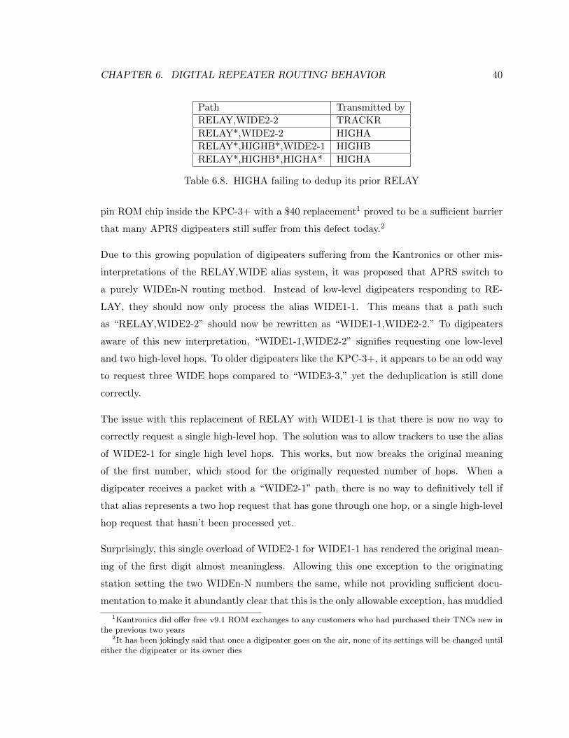
firmware ROM regarding the deduplication behavior just presented [19].
The KPC-3+ correctly deduplicated packets routed via the WIDEn-N system, but failed to
correctly add to or consult the dedup hash table for single-hop aliases such as RELAY. This
meant that popular routing paths such as “RELAY,WIDE2-2” would still result in routing
loops on the network:
Kantronics did release a patched ROM v9.1 in 2007, but to insufficient effect. Getting
access to digipeaters at remote radio sites is burdensome, and physically replacing the 32
CHAPTER 6. DIGITAL REPEATER ROUTING BEHAVIOR 40
Path Transmitted by
RELAY,WIDE2-2 TRACKR
RELAY*,WIDE2-2 HIGHA
RELAY*,HIGHB*,WIDE2-1 HIGHB
RELAY*,HIGHB*,HIGHA* HIGHA
Table 6.8. HIGHA failing to dedup its prior RELAY
pin ROM chip inside the KPC-3+ with a $40 replacement1 proved to be a sufficient barrier
that many APRS digipeaters still suffer from this defect today.2
Due to this growing population of digipeaters suffering from the Kantronics or other mis-
interpretations of the RELAY,WIDE alias system, it was proposed that APRS switch to
a purely WIDEn-N routing method. Instead of low-level digipeaters responding to RE-
LAY, they should now only process the alias WIDE1-1. This means that a path such
as “RELAY,WIDE2-2” should now be rewritten as “WIDE1-1,WIDE2-2.” To digipeaters
aware of this new interpretation, “WIDE1-1,WIDE2-2” signifies requesting one low-level
and two high-level hops. To older digipeaters like the KPC-3+, it appears to be an odd way
to request three WIDE hops compared to “WIDE3-3,” yet the deduplication is still done
correctly.
The issue with this replacement of RELAY with WIDE1-1 is that there is now no way to
correctly request a single high-level hop. The solution was to allow trackers to use the alias
of WIDE2-1 for single high level hops. This works, but now breaks the original meaning
of the first number, which stood for the originally requested number of hops. When a
digipeater receives a packet with a “WIDE2-1” path, there is no way to definitively tell if
that alias represents a two hop request that has gone through one hop, or a single high-level
hop request that hasn’t been processed yet.
Surprisingly, this single overload of WIDE2-1 for WIDE1-1 has rendered the original mean-
ing of the first digit almost meaningless. Allowing this one exception to the originating
station setting the two WIDEn-N numbers the same, while not providing sufficient docu-
mentation to make it abundantly clear that this is the only allowable exception, has muddied
1Kantronics did offer free v9.1 ROM exchanges to any customers who had purchased their TNCs new inthe previous two years
2It has been jokingly said that once a digipeater goes on the air, none of its settings will be changed untileither the digipeater or its owner dies
CHAPTER 6. DIGITAL REPEATER ROUTING BEHAVIOR 41
the waters as to the actual meaning of the first number. Based on a sample of 21 million
packets on the APRS-IS world-wide APRS backbone on May 8th, 2014, it was found that
0.7% of APRS packets requested routing paths such as WIDE1-2 or WIDE2-3, which should
not ever exist before or after the WIDE2-1 exception was made.. A station beaconing with
a path of WIDE2-3 indicates that they are requesting two hops, and three of those hops
are remaining, which is nonsense.3 This demonstrates that users are clearly confused and
that a major institutional failure has occurred in how the meaning of the WIDEn-N alias
has been presented.
6.5 Minimum WIDEn-N Behavior
APRS digipeaters are divided into two classes: high-level digipeaters and low-level digi-
peaters, which dictates variations in their behavior. High-level digipeaters form the ma-
jor backbone of the APRS digipeater network and are generally installed on the tops of
mountains, tall office buildings, and large towers. Low-level digipeaters usually have their
antennas less than 50 feet above ground level, and cover a small subset of the wider coverage
provided by the nearest high-level digipeater.
Since each low-level digipeater’s coverage area is a subset of the nearest high-level digi-
peater’s coverage, a low-level digi isn’t needed to repeat packets coming in from the high-
level digipeater. Low-level digipeaters are designed to solely act as “boosters” to help local
low-power trackers be able to reach the nearest high-level digi. Therefore, low-level digi-
peaters should only digipeat packets which have “WIDE1-1” as their first routing hop, since
that indicates that the user doesn’t believe they can reach high-level digipeaters directly.
High-level digipeaters form the actual blanket coverage of APRS, and should respond to any
valid WIDEn-N alias which still contains unconsumed hops, including WIDE1-1. This is
because many digipeaters will only consume the first unused alias in the path, so a low-power
tracker that gets “lucky” and manages to reach a high-level digipeater while using a path
such as “WIDE1-1,WIDE2-2” depends on high-level digipeaters responding to WIDE1-1.
Digipeater behavior includes several more caveats which don’t involve the APRS WIDEn-N
3The proper way to request three hops would be to use WIDE3-3.
CHAPTER 6. DIGITAL REPEATER ROUTING BEHAVIOR 42
routing alias,4 so this section can’t be considered a complete definition of a digipeater’s
behavior.
6.6 Variations on Digipeater Behavior
As previously mentioned, the failure of the APRS specification to provide a comprehensive
extension of digipeater behavior for APRS has caused implementers to get creative with
the details and extensions of the basic behavior defined in the AX.25 specification. Some
of these variations include:
• How should the last hop of multi-hop aliases be handled?5
• Preemptive digipeating, where digipeaters consider all unused aliases, instead of only
the first, and possibly consumes multiple hop requests if an alias match is found later
in the path.
• Long path traps, where abusive WIDE paths such as WIDE7-7 are trapped and all
or many requested hops are consumed by the first digipeater, to prevent flooding
extremely large areas.
• Direct-only digipeaters, where low-level digipeaters don’t only respond to WIDE1-1,
but only digipeat packets when they appear to have not been already digipeated by
another digipeater.
• Viscous delay digipeaters, where packets are held for a number of seconds to see if
they are otherwise re-transmitted by other digipeaters. If an echo of a packet is heard,
it gets dropped instead of digipeated.
• Token bucket digipeaters, which refuse to digipeat stations which exceed a specified
volume of network traffic.
While the implications of any single item on this list are seemingly small, the countless
permutations and inconsistencies seen deployed in the world-wide APRS network causes
4Examples include the expectation of digipeaters to substitute their callsigns into routing paths as theyconsume aliases, and that they still must respond to their callsign as a routing hop in addition to theWIDEn-N alias.
5i.e. should “WIDE3-1” become “DIGIA*” or “DIGIA*,WIDE3*”?
CHAPTER 6. DIGITAL REPEATER ROUTING BEHAVIOR 43
the network to behave unpredictably and give disappointing levels of service to its end-
users. Further work is needed to specify how much of a digipeater’s behavior is required
versus optional, and how much latitude should be given to individual digipeater operators
for any of the optional features implemented.

OSI Layer 3 — Network
44
7 Node Beaconing Behavior
Since APRS is a source-routed protocol, most of the decisions as to how often a station
should send traffic and how far that traffic should travel are allowed to be made by the
originating station. The existing specification for the protocol hardly touches on this issue,
while a great deal of time and energy is spent on the development forums bemoaning specific
examples of misbehaving members of the network. The two major parameters under the
source node’s control that are considered here are the frequency of beaconing and the routing
path used for each beacon.
Being a source-routed protocol does fundamentally introduce a moral hazard in the network.
For each node in the network to enjoy the most benefit from the network, they would want
to beacon as often as possible with the longest path allowed by the network. It is only
by mutual trust, respect, and education that this logic isn’t universally followed and the
network is not grossly oversubscribed in the self-interest of every individual network node.
Unfortunately, the most popular documentation on APRS fails to stress the importance of
correctly configuring nodes in the best interest for the network at large, and rarely gives
any concrete guidance on what values should typically be used when configuring various
types of network nodes.
7.1 Beaconing Algorithms
For each APRS node with information available for the network, a local decision needs
to be made as to when that information will best serve the local network and should be
transmitted. This is rarely a trivial decision, and one that could warrant much more creative
and application or data specific solutions than the ones presented here, which should be
considered the typical minimum of most popular APRS trackers. The only datum considered
45
CHAPTER 7. NODE BEACONING BEHAVIOR 46
in this work is that of a mobile node’s position, but these algorithms would likely extend
to most other user applications of APRS.
7.1.1 Fixed Interval Beaconing
The simplest beaconing algorithm consists of waiting a single fixed interval between beacons,
and only requires a single parameter that is the beacon interval. When a tracker is turned
on, it acquires a GPS lock and immediately sends out a beacon and starts a timer. Once
that timer exceeds the beacon interval value, a new position is acquired from the GPS
receiver and the new location is beaconed. While simple, this algorithm does suffer from a
number of inadequacies:
• The decision to beacon is made solely based on how long it has been since the previous
beacon, without considering any other information available to the tracker. Examples
of additional information would include whether the tracker has moved, how fast the
tracker is moving, or any packets received from the APRS network since the last
beacon.
• A single fixed interval limits the amount of entropy introduced into the network with
regards to inter-packet arrival at other nodes. Since APRS is a CSMA shared channel
network, it’s tempting to use Poisson distribution models for network capacity, which
is likely invalid when the only source of entropy per tracker is the time when it was
last turned on or gained GPS lock. This is discussed further in the next chapter.
There are of course several possible extensions to the fixed interval beaconing algorithm
which each fix various deficiencies at the expense of simplicity.
7.1.2 Time Slot Interval Beaconing
Arguably a more restrictive form of fixed interval beaconing, time slotting is based on the
idea of preventing channel collisions by allocating each tracker a fixed time slot in each
interval for when they are allowed to transmit. An unfeasible solution for the national
APRS network due to its scale and lack of coordination, time slotting is often applied

CHAPTER 7. NODE BEACONING BEHAVIOR 47
where unusually high levels of coordination do exist, such as special events and insular
networks.
Time slotting introduces a new parameter called the slot time, and depends on every tracker
using it having synchronized real time clocks, which is reasonable since most GPS receivers
provide real time to within typically 200ms of UTC as part of their position reports.1
The slot time determines how many seconds after the beginning of each interval a tracker
should beacon. The beginning of each interval is defined by the top of the UTC hour,2 and
intervals run successively for the remainder of the hour. For example, a tracker configured
to time slot with an interval of 550 seconds and a time slot of 12 would beacon at the
following times:
Time Calculated by
00:00:12 0*550 + 12
00:09:22 1*550 + 12
00:18:32 2*550 + 12
00:27:42 3*550 + 12
00:36:52 4*550 + 12
00:46:02 5*550 + 12
00:55:12 6*550 + 12
01:00:12 0*550 + 12
This deterministic beaconing algorithm allows carefully designed networks to over-subscribe
network throughput well beyond the levels expected from the national APRS channel with
its stochastic access methods. On an insular network separate from the national network, it
would be possible to set an aggressively short beacon interval and carefully space trackers
such that no two beacons collide with each other. This would make it possible to accomplish
service levels such as every-minute position updates from several dozen tracked vehicles, at
the expense that there is no allowance for any additional traffic on the RF channel, and
the network would depend on manual assurance that every tracker is configured to use its
proper time slot.
1The 200ms uncertainty is a typical value due to the delivery of time over an asynchronous 4800 baudserial port. Internally, GPS receivers must maintain their real time clocks to several orders of magnitudehigher precision than this to be even remotely useful, but this precision isn’t needed for APRS time slotting.
2Specifying to use UTC time is remarkably important, since UTC and GPS time have currently divergedby 16 seconds due to only UTC including leap seconds. Most, but not all, GPS receivers correctly compensatefor this variable offset and report correct UTC time in their GPRMC sentences.
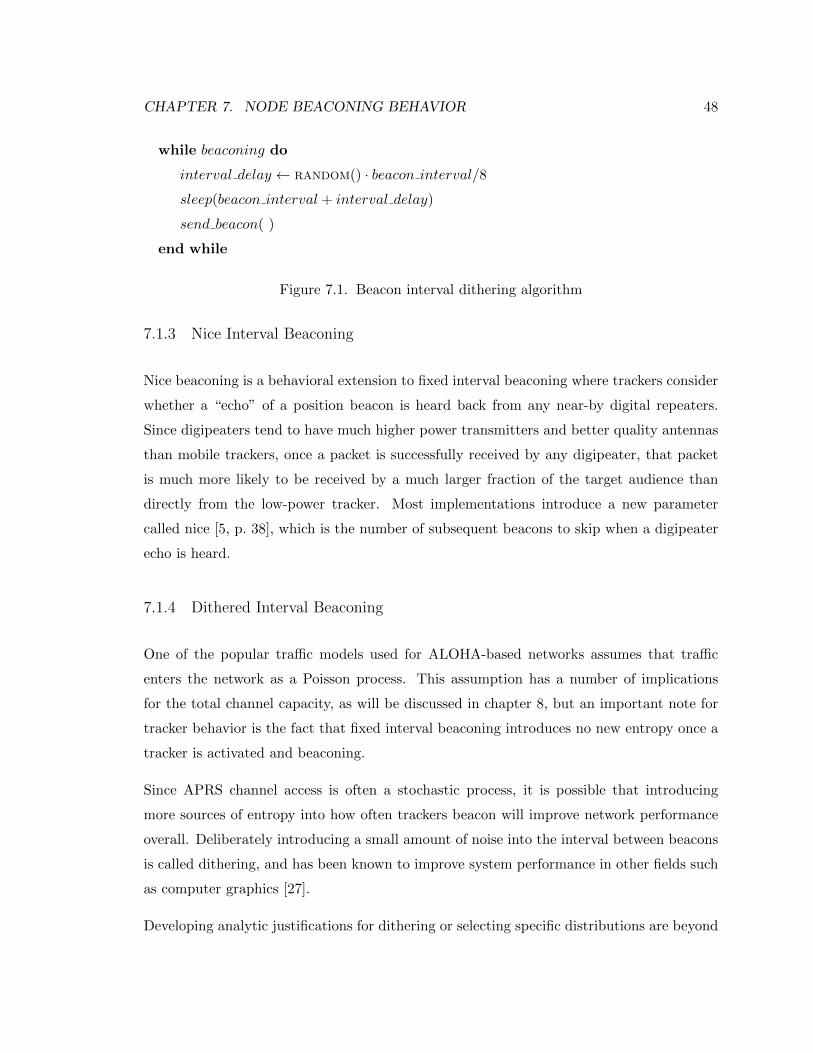
CHAPTER 7. NODE BEACONING BEHAVIOR 48
while beaconing do
interval delay ← random() · beacon interval/8sleep(beacon interval + interval delay)
send beacon( )
end while
Figure 7.1. Beacon interval dithering algorithm
7.1.3 Nice Interval Beaconing
Nice beaconing is a behavioral extension to fixed interval beaconing where trackers consider
whether a “echo” of a position beacon is heard back from any near-by digital repeaters.
Since digipeaters tend to have much higher power transmitters and better quality antennas
than mobile trackers, once a packet is successfully received by any digipeater, that packet
is much more likely to be received by a much larger fraction of the target audience than
directly from the low-power tracker. Most implementations introduce a new parameter
called nice [5, p. 38], which is the number of subsequent beacons to skip when a digipeater
echo is heard.
7.1.4 Dithered Interval Beaconing
One of the popular traffic models used for ALOHA-based networks assumes that traffic
enters the network as a Poisson process. This assumption has a number of implications
for the total channel capacity, as will be discussed in chapter 8, but an important note for
tracker behavior is the fact that fixed interval beaconing introduces no new entropy once a
tracker is activated and beaconing.
Since APRS channel access is often a stochastic process, it is possible that introducing
more sources of entropy into how often trackers beacon will improve network performance
overall. Deliberately introducing a small amount of noise into the interval between beacons
is called dithering, and has been known to improve system performance in other fields such
as computer graphics [27].
Developing analytic justifications for dithering or selecting specific distributions are beyond

CHAPTER 7. NODE BEACONING BEHAVIOR 49
the scope of this work, but it’s theorized that introducing any kind of entropy with approx-
imately 1% variance could improve network traffic distribution. Figure 7.1 shows a possible
implementation, where RANDOM() is a function that returns a normalized distribution
such as a uniform distribution in the range [0,1] or a Gaussian distribution with µ = 0 and
σ = 1. The dividing factor of 8 was selected to scale the uniform distribution [0,1] to yield
a variance of 1%, but that value was selected arbitrarily.
7.1.5 SmartBeaconing
SmartBeaconing™is an adaptive beaconing algorithm developed by Tony Arnerich and Steve
Bragg for the HamHUD tracker kits [7]. It allows trackers to make intelligent decisions as
to how often to beacon based on how “interesting” the tracker’s new position is. Vehicles
moving in straight lines will tend to beacon at very long intervals, but will beacon more often
when making turns or traveling faster. The algorithm is owned by HamHUD Nichetronix,
LLC, and licensed freely for non-commercial amateur radio applications.
This algorithm is particularly useful for APRS due to the fact that APRS position reports
support dead-reckoning, where they include a direction and velocity. As long as trackers
don’t deviate from this advertised heading, there is less reason to repeatedly beacon the
tracker’s new position.
The SmartBeaconing algorithm accepts up to seven parameters from the user[23], which are
relatively more opaque than the one or two parameters required for all the other popular
interval algorithms. While there are suggested default values for each of these parameters,
SmartBeaconing still proves to be controversial due to its users tending to beacon much
more often than trackers using other beaconing algorithms[8]. As discussed in chapter 8,
calculating the actual channel capacity in an area and the appropriate beaconing interval
for any of these algorithms are not at all straight forward.
The original HamHUD algorithm is documented online as a snippet of C-like pseudo-code
as shown in figure 7.2. In addition to the seven algorithm parameters, the pseudo-code
requires the current speed and heading of the tracker, which are both typically available
from the $GPRMC NMEA sentence [13] provided by the tracker’s GPS receiver, and the
number of seconds since the last transmitted beacon. Unfortunately, there are a number of

CHAPTER 7. NODE BEACONING BEHAVIOR 50
Parameter Name Value Description
low speed 5 mph This is the speed below which the trackerswitches to the slow beacon interval and nolonger performs corner pegging.
slow beacon interval 1800 seconds This is how often a tracker should beacon whenit is moving slower than low speed, which indi-cates that it is essentially stopped.
high speed 60 mph High speed is the value that slower speed beaconintervals are interpolated from. Speeds fasterthan high speed are valid but simply beacon atfast beacon interval.
fast beacon interval 180 seconds This is how often a tracker should beacon whentraveling at high speed and the scalar used tocalculate beacon intervals at lower speeds as afraction of high speed.
turn minimum 30° The absolute minimum heading change neededto trigger a “corner peg” where the tracker bea-cons sooner than its speed warrants.
turn slope 255°miles / hr A scalar to convert between how fast a tracker isgoing and how tight of a turn they need to per-form to trigger a corner peg. The original doc-umentation notes this value as unitless, whichisn’t entirely invalid since degree miles per hourisn’t a particularly helpful dimension.
turn beacon interval 15 seconds The minimum time between beacons when atracker is changing heading often.
Table 7.1. Suggested defaults for SmartBeaconing parameters

CHAPTER 7. NODE BEACONING BEHAVIOR 51
issues with the provided code that have possibly harmed deployment of the SmartBeaconing
algorithm on other trackers:
• Variable names change. Both “speed” and “mph” are used to indicate the current
speed of the tracker.
• Variable names are inconsistent. slow rate is used for the beacon interval when the
vehicle is stopped, fast beacon rate for when the vehicle is moving, and turn time for
when it is turning. A better set of variable names could be * beacon interval.
• The corner pegging algorithm suffers from an off-by-one error due to the final if
statement being a > comparison instead of a ≥ comparison. As documented, turning
a corner would never cause an early beacon.
• The corner pegging section changes the value of secs since beacon instead of bea-
con rate, where secs since beacon is a system invariant that could possibly be imple-
mented as a macro or function call.
• The SmartBeaconing documentation specifies that the velocities used are in units of
miles per hour, where velocities expressed in the APRS protocol are in knots.3
Due to these issues, it seemed appropriate to rewrite the algorithm to correct these issues
and to re-typeset the pseudo-code in a more contemporary style, which can be seen in
figure 7.3.
7.2 Path Recommendations
In addition to the task of deciding when to beacon, each user needs to make a judgment as
to how far they want to flood their traffic throughout the APRS network. This is another
subject that evokes controversy due to the problem that recommendations that are valid in
most of the network will often be invalid for small parts of it. This causes every discussion
on the subject to be muddied with arguments about small edge-cases and the specifications
make no concrete recommendations on the subject all together.
3APRS uses knots for velocity due to most GPS receivers outputting location data as NMEA 0183sentences, which were originally designed for maritime applications.
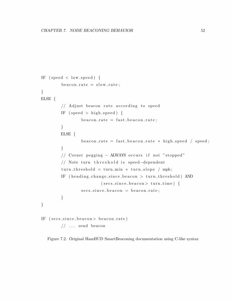
CHAPTER 7. NODE BEACONING BEHAVIOR 52
IF ( speed < low speed ) {beacon rate = s l o w r a t e ;
}ELSE {
// Adjust beacon ra t e accord ing to speed
IF ( speed > high speed ) {beacon rate = f a s t b e a c o n r a t e ;
}ELSE {
beacon rate = f a s t b e a c o n r a t e ∗ high speed / speed ;
}// Corner pegging − ALWAYS occurs i f not ” stopped ”
// Note turn t h r e s h o l d i s speed−dependent
t u r n t h r e s h o l d = turn min + t u r n s l o p e / mph;
IF ( head ing change s ince beacon > t u r n t h r e s h o l d ) AND
( s e c s s i n c e b e a c o n> turn t ime ) {s e c s s i n c e b e a c o n = beacon rate ;
}}
IF ( s e c s s i n c e b e a c o n> beacon rate )
// . . . send beacon
Figure 7.2. Original HamHUD SmartBeaconing documentation using C-like syntax
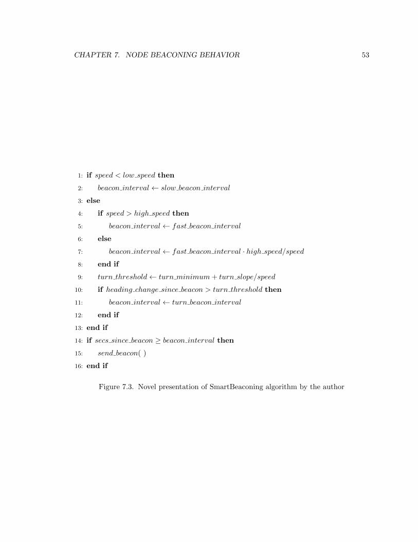
CHAPTER 7. NODE BEACONING BEHAVIOR 53
1: if speed < low speed then
2: beacon interval← slow beacon interval
3: else
4: if speed > high speed then
5: beacon interval← fast beacon interval
6: else
7: beacon interval← fast beacon interval · high speed/speed8: end if
9: turn threshold← turn minimum+ turn slope/speed
10: if heading change since beacon > turn threshold then
11: beacon interval← turn beacon interval
12: end if
13: end if
14: if secs since beacon ≥ beacon interval then15: send beacon( )
16: end if
Figure 7.3. Novel presentation of SmartBeaconing algorithm by the author
CHAPTER 7. NODE BEACONING BEHAVIOR 54
This means that the following guidance is guaranteed to be “flawed” when applied some-
where in the APRS network, but the hope is that this will be generally correct when consid-
ering most of the network. The local administrators in regions which require different path
selections than the following should be expected to either maintain and publish a set of
their own recommendations or re-design their network to support the standard suggestions.
7.2.1 Vehicles and Mobile Stations
In the most general case, vehicles should use a path of “WIDE1-1,WIDE2-1,” which requests
two total hops, including allowing low-level digis to assist them reaching the high-level
digipeater network on their first hop. Vehicles which stay in highly populated areas should
consider using the shorter “WIDE1-1” path, while vehicles which do the opposite and spend
a significant amount of their time in areas with unusually sparse APRS coverage may use
“WIDE1-1,WIDE2-2.” [14]
7.2.2 Fixed Stations
Many APRS stations aren’t expected to ever move, such as home stations acting as Internet
gateways, digipeaters that are part of the infrastructure, or remote weather stations. Since
these stations should have the transmitter power and high-quality antennas needed to reach
high-level digipeaters, they should not begin their path with WIDE1-1 but select between
the following options depending on how many hops are needed:
• WIDE2-1 - A single hop for unimportant traffic or stations near a particularly large
coverage digipeater.
• WIDE2-2 - The most standard path that stations should only deviate from after
careful consideration.
• WIDE3-3 - Should only be used in mountainous or sparse areas for traffic important
to a large number of stations. Very few stations should ever use this path.
Unlike mobile trackers, fixed stations enjoy the advantage that they do not need to handle
a constantly changing APRS infrastructure. Instead of using the APRS WIDE aliases,
CHAPTER 7. NODE BEACONING BEHAVIOR 55
fixed stations should seriously consider using literal paths consisting of specific digipeater
callsigns. For example, a fixed station desiring a single hop through the near-by HIGHA
digipeater should beacon with a path of “HIGHA” instead of “WIDE2-1.” This causes only
the HIGHA digipeater to repeat the packet and not involve any further away or lower-level
digipeaters which happen to also decode the initial transmission. Literal paths requesting
the help of specific digipeaters is rarely seen in APRS traffic, but should be encouraged.
Fixed stations should also consider using “proportional pathing,” which warrants its own
section below.
7.2.3 Airborne Stations
APRS is often used as a safety or recovery system for airplanes or weather balloons, and
these stations MUST NOT use any digipeaters in their path while significantly above
ground-level. [15] It is critical that airborne stations use an empty path because their
altitude ensures that they already cover more area than any of the digipeaters they would
enlist to repeat their traffic. It is common for balloons to be launched with paths such as
“WIDE1-1,WIDE2-1” which cause havoc as packets are received by every digipeater within
hundreds of miles and needlessly repeated to other stations which have already received the
original transmission.
It may be desirable for airborne trackers to support the feature of switching from an empty
path to something else when on the ground. A good example would be a weather balloon
payload switching from an empty path to a “WIDE1-1” path when the balloon bursts to
aid in recovery of the payload once it reaches the ground.
7.2.4 Proportional Pathing
Proportional pathing is the tracker behavior where every beacon does not use the same
routing path, which is the norm for APRS trackers. It is not a part of the APRS spec, but
has been documented as an errata on the aprs.org website. [11] Since information passed
through the APRS network is usually more important for stations near the originating
station than those further away, it follows that it would be preferable for near-by stations
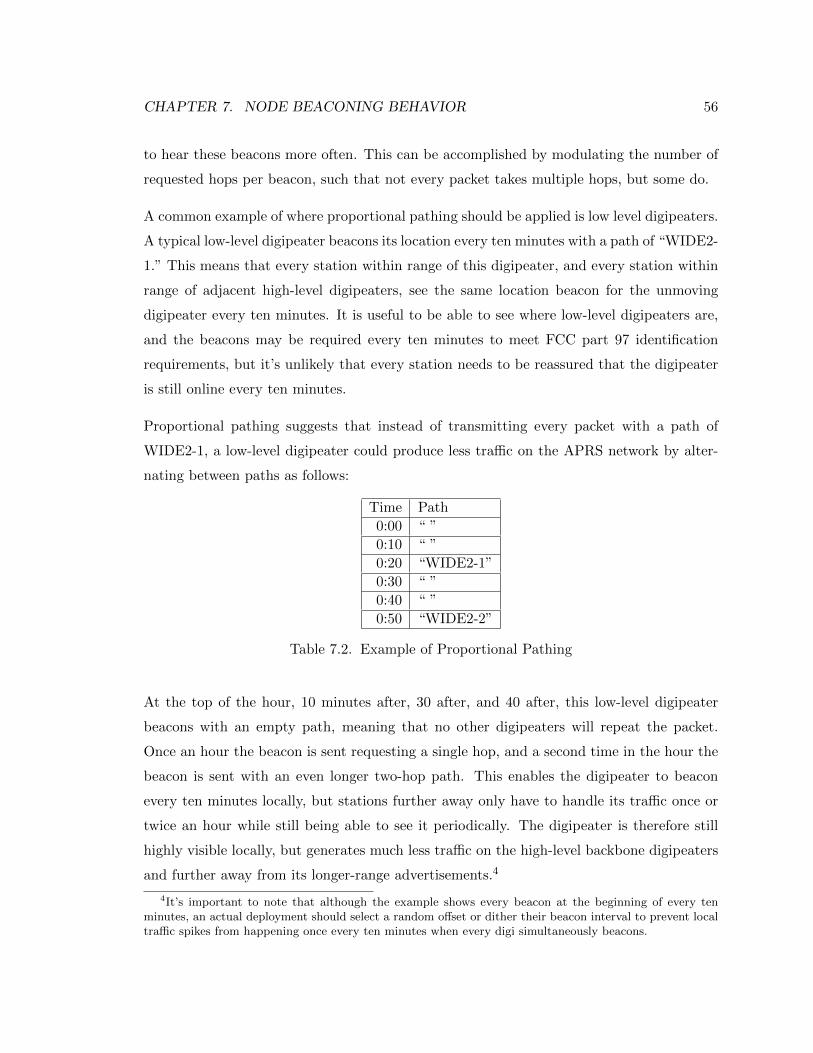
CHAPTER 7. NODE BEACONING BEHAVIOR 56
to hear these beacons more often. This can be accomplished by modulating the number of
requested hops per beacon, such that not every packet takes multiple hops, but some do.
A common example of where proportional pathing should be applied is low level digipeaters.
A typical low-level digipeater beacons its location every ten minutes with a path of “WIDE2-
1.” This means that every station within range of this digipeater, and every station within
range of adjacent high-level digipeaters, see the same location beacon for the unmoving
digipeater every ten minutes. It is useful to be able to see where low-level digipeaters are,
and the beacons may be required every ten minutes to meet FCC part 97 identification
requirements, but it’s unlikely that every station needs to be reassured that the digipeater
is still online every ten minutes.
Proportional pathing suggests that instead of transmitting every packet with a path of
WIDE2-1, a low-level digipeater could produce less traffic on the APRS network by alter-
nating between paths as follows:
Time Path
0:00 “ ”
0:10 “ ”
0:20 “WIDE2-1”
0:30 “ ”
0:40 “ ”
0:50 “WIDE2-2”
Table 7.2. Example of Proportional Pathing
At the top of the hour, 10 minutes after, 30 after, and 40 after, this low-level digipeater
beacons with an empty path, meaning that no other digipeaters will repeat the packet.
Once an hour the beacon is sent requesting a single hop, and a second time in the hour the
beacon is sent with an even longer two-hop path. This enables the digipeater to beacon
every ten minutes locally, but stations further away only have to handle its traffic once or
twice an hour while still being able to see it periodically. The digipeater is therefore still
highly visible locally, but generates much less traffic on the high-level backbone digipeaters
and further away from its longer-range advertisements.4
4It’s important to note that although the example shows every beacon at the beginning of every tenminutes, an actual deployment should select a random offset or dither their beacon interval to prevent localtraffic spikes from happening once every ten minutes when every digi simultaneously beacons.
CHAPTER 7. NODE BEACONING BEHAVIOR 57
This example considered the most common form of proportional pathing, where the tracker
maintains a finite state machine to switch between a limited and predefined list of paths,
but a possible area for future work would be to develop more sophisticated proportional
pathing algorithms. Much like the SmartBeaconing algorithm considered earlier, heuristics
could be developed to categorize how important the next beacon will be, based on variables
such as the local traffic level, how many new stations have been recently heard, or time of
day, and used to adaptively change the routing path used.
7.3 Conclusion
This chapter has presented a list of the most popular algorithms used to determine when a
tracker should beacon, and provided some general guidance on what routing paths should be
used by different types of trackers. The source-routed nature of APRS is often considered
a double-edge sword, since any operator may tailor how the network handles the local
station’s traffic to meet their own need. The downside to source-routing is that malicious
or ignorant stations are empowered to cause a tremendous amount of harm to the network’s
performance. There are inevitable exceptions to the guidance given in this chapter, so
modifications to any defaults should be done with careful consideration and user education.
The guidance given has been as general as possible, without documenting the numerous edge
cases and exceptions in individual areas. This is a common flaw with APRS documentation,
where writers refuse to give any concrete advice since it is inevitably wrong somewhere in the
world-wide APRS network. Stations planning to operate in unusually high or low density
areas should carefully consider their beaconing behavior and consult local APRS interest
groups.5
5http://info.aprs.net is a particularly useful website documenting local exceptions to these generalrules.
8 APRS RF Channel Capacity
One of the largest limitations of the APRS network is the fact that it primarily operates
on a single regional 1200 bits per second data channel. Individual nodes share the 1200bps
channel using CSMA, as discussed in section 3.4, but the relationship between these channel
access methods and how often a station should beacon isn’t straight forward.
The APRS specification avoids giving concrete guidance on what beacon interval should be
used beyond stating that every station should beacon at the net’s cycle rate, which it lists as
10 minutes locally and 30 minutes network wide[33, p. 9].1 For fixed nodes such as weather
stations and network infrastructure, these intervals are appropriate since their information
for the network is unlikely to dramatically change in the 10 to 30 minute time scale. Mobile
users are a different story, since they often have new information for the network such as
a direction change or a new text message. Fixed 10 minute beacon intervals are therefore
often unsatisfactory for mobile users, who would like to see new information passed to the
rest of the network more quickly. The popularity of SmartBeaconing is a testament to
this desire to beacon more often, but the question now becomes how much more often can
stations beacon while staying within the limitations of the APRS network?
This chapter will give an introduction to the original ALOHAnet research that networks
like APRS are based on, and point out how these models fall short of the actual APRS
network. A comprehensive study of the specifics as applied to APRS are beyond the scope
and resources of this work, so no concrete recommendations will be made in this chapter.
1see proportional pathing in the previous section
58
CHAPTER 8. APRS RF CHANNEL CAPACITY 59
8.1 Network Capacity Objectives
The stated objective of APRS is to pass real-time tactical information among a station’s
60 nearest peers. This value was apparently selected arbitrarily based on the feeling that it
is unlikely that a station would need to interact with anyone beyond their 60 closest peers,
but will nevertheless be used for the analysis in this chapter. This does complicate analysis
of the APRS network since each station’s set of their 60 nearest peers, which is referred
to as their “Aloha Circle,” is a different subset of all the stations in the network. Every
station has a different concept as to who is in their Aloha Circle and who is not. Analysis
is further complicated by the fact that few APRS stations are actually within radio range
of 60 other stations, so often a significant portion of an Aloha Circle is beyond the local
horizon and relayed through a limited number of digipeaters. This effects a phenomenon
called the “hidden node problem,” which impacts Layer 1 CSMA access, which is ignored
in the limited scope of this chapter.
An appropriate starting point for analyzing APRS channel capacity would be the original
methods developed for the ALOHA System at the University of Hawaii[1]. The ALOHAnet
was a 9600bps UHF packet radio system that was the first application of wireless computer
networking. This system developed several of the shared channel access methods that would
subsequently be used in other protocols such as Ethernet, GSM, and APRS.
8.2 Poisson Channel
The most basic analysis of a channel’s Aloha Circle capacity can be based on the assumption
that each packet is the same length, that traffic enters the network as a Poisson process, and
that any collision between two packets causes both of them to fail to be delivered. Defining
the rate of packets entering the network as λ packets per second and the length of each
packet as τ seconds, the normalized channel traffic G can be calculated as
G = λτ (8.1)
This normalized channel traffic metric is expressed using the dimensionless unit Erlang
named after the engineer who originally developed the field of queuing theory as applied to
the telephone network. Erlangs express the fraction of a channel that would be needed for
CHAPTER 8. APRS RF CHANNEL CAPACITY 60
all of the traffic entering the network. For example, a value G = 1.0 would indicate that a
single station would need to transmit packets continuously, where G = 0.5 indicates that
the channel is idle half of the time. Erlang values above 1.0 are valid, and simply represent
that more than one channel would be required to handle all of the traffic.
When channel access is stochastic, as it is in APRS, there is no guarantee that two stations
won’t transmit at the same time, regardless of how much traffic there is on the network.
Any packet transmission starting less than τ seconds before or after another would cause
a collision and simple models dictate that both packets would be lost. This indicates that
the rate of successfully received packets exiting the network is often less than λ, and is
traditionally notated as λ′. Since λ′ ≤ λ, we define the normalized channel throughput S as
S = λ′τ (8.2)
This implies that the fraction of the channel capacity used for successfully delivered packets
must follow the same relationship as λ and λ′, namely that S ≤ G.
Making the assumption that channel access is Poisson in nature, the probability that a
packet will collide with another can be derived to be e−2λτ , as originally derived by Abram-
son [1]. This yields the relationship between S and G of
S = Ge−2G (8.3)
This indicates a moderately surprising result that for Poisson channel access, the throughput
is completely independent of the number of stations on the channel, but only dependent
upon the total channel loading.
Graphing the channel throughput versus the channel’s traffic yields figure 8.1, which in-
dicates that as you increase channel traffic, throughput increases to an inflection point
when there is no unused channel capacity and packet collisions finally start to dominate the
channel and harm throughput. This inflection point happens to be at an incoming traffic
G = 0.5 which yields an expectation that 36% of the packets will be successfully received
(S = 0.18).
While assuming that APRS traffic is based on a Poisson process is highly suspect, this
simple model of channel capacity does yield some insightful values. Collecting several days
of APRS traffic on 144.390MHz in San Luis Obispo, California shows an average packet
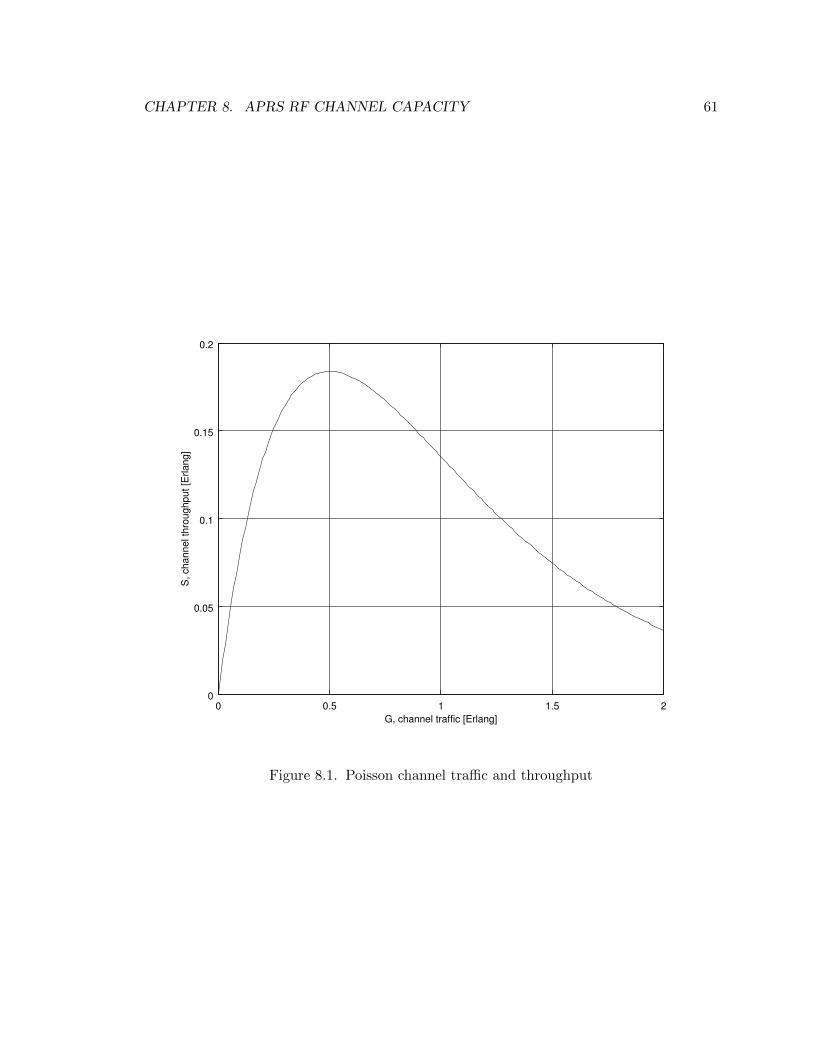
CHAPTER 8. APRS RF CHANNEL CAPACITY 61
0 0.5 1 1.5 20
0.05
0.1
0.15
0.2
G, channel traffic [Erlang]
S, cha
nnel th
rou
ghp
ut [E
rlan
g]
Figure 8.1. Poisson channel traffic and throughput
CHAPTER 8. APRS RF CHANNEL CAPACITY 62
size of 119 octets. With a typical 300ms preamble, the assumption that every packet is the
mean length, and a data rate of 1200bps, this yields τ = 1.09 seconds.
λAPRS =GMAX
τ= 0.457 (8.4)
Equation 8.4 indicates that a single APRS channel can support 0.457 transmitted packets
per second, or 27 packets per minute, which need to be shared between all of the partic-
ipating network nodes. Assuming the typical target LAN size of 60 stations, this implies
an average packet interval per station of 2 minutes 13 seconds.2 The less satisfying result
is the fact that only 10 of these packets every minute will be successfully received, which
indicates that two thirds of the transmitted power is wasted.
The next section will go into how this Poisson model is deficient to the point that this 2
minute 13 seconds value is nearly meaningless. Any station that beaconed that fast on an
actual APRS network could very quickly be identified as abusive to the rest of the network,
so further work is needed before an analytic interval suggestion can be made. What this
calculation does demonstrate is that the general concept of 60 stations sharing a single
ALOHA channel in the way APRS intends is within the realm of possibilities. Had this
value come out an order of magnitude larger, the claim that APRS could allow a user to
discover 60 other stations would be much more suspect.
8.3 Deficiencies of the Poisson Model
There were several assumptions made to simplify the just-presented model for an ALOHA
channel that are not valid when applied to a typical APRS network. While most of these
assumptions indicate that the result of equation 8.4 is overly optimistic and stations should
beacon less often, there are enough conflicting mechanisms at play in both directions that
the true traffic versus throughput relationship does not appear to be easily found and
requires further work beyond this paper. Some of the issues ignored in this chapter include:
• Differences in packet length – Actual APRS traffic varies in length, which has an effect
on throughput rates by changing τ . Abramson presented a closed solution for the case
2For the reader skimming this chapter, DO NOT use this beacon interval for APRS; this Poisson modelis too simplified to give meaningful results. A suggested default is 600 second intervals when beaconing.
CHAPTER 8. APRS RF CHANNEL CAPACITY 63
of two discrete packet lengths [1], but his methods don’t lend themselves well to the
broad distribution of packet lengths found in APRS. His solution does imply that
users should attempt to make packets as short as possible to improve throughput.
• Digipeaters and channel access methods – The presented model assumes that every
packet is added to the channel as an entirely blind shot in the dark, but many APRS
stations use CSMA to avoid transmitting on already busy channels. This reduces
the window for destructive collisions and thus reduces the ratio between the channel
traffic G and the usable throughput S.
• FM capture effect – This model assumed that any overlap between packets is fatal
for both packets, but experience shows that packets from closer stations often “beat
out” overlapping packets from stations much further away. This effect has not been
quantified as it pertains to APRS.
• Sources of entropy in the network – Starting with a Poisson stochastic model implies
a strong assumption that every packet starts at a random time independent of every
other packet. Many APRS stations beacon on a fixed interval, such as 600 seconds,
which makes that station’s traffic very self-similar. Digipeaters also strongly break this
assumption by their action of immediately repeating packets after they’re originally
transmitted. These digipeater echos aren’t random at all. Papers have been written
on the misuse of Poisson traffic models with regards to TCP/IP networks [26], and
those arguments often apply equally well to the APRS network.
• The heterogeneous nature of APRS equipment – Any closed-form analysis of APRS
depends on each network node behaving in one of a small set of possible behaviors. The
home-brewed and come-as-you-are nature of APRS makes the cumulative behavior of
the network at large much harder to model. Useful models would need to depend on
careful measurement of the behavior of existing nodes, and likely use Monte Carlo
methods to make meaningful statements about the system at large.
In the end, building a meaningful model for APRS network traffic will likely prove to be
surprisingly challenging. Much of this derives from the unusual amount of latitude given
to APRS implementations by the lack of detailed specifications that causes the aggregate
network to behave so unpredictably. For further work modeling APRS to deliver meaningful

CHAPTER 8. APRS RF CHANNEL CAPACITY 64
results, it’s likely that it will need to begin by making a decision on which existing nodes
in the APRS network are “misbehaving” by some developed metric and exclude them from
any further analysis.
The community has been extremely reluctant to outright classify APRS hardware as mis-
behaving in the past, due to the embedded nature of APRS nodes that usually precludes
any major modifications in behavior of existing nodes. Classifying a node as misbehav-
ing often meant that the operator would need to spend a significant amount of time and
money outright replacing the deficient hardware. As more APRS nodes move to open-source
and/or reprogrammable implementations, it’s conceivable that updates to APRS behavior
as resulting from future research may become merely difficult, instead of utterly impossible.3
3For example, the open source aprx package is one of the most popular pieces of i-gate software on thenetwork [25], and modern trackers like those from Argent Data often enjoy firmware updates which arerelatively easy to install.
9 Conclusion
This paper has considered several of the different aspects of the APRS network, ranging from
the low-level modem and channel access methods up to how nodes should make beaconing
and routing decisions. During this survey, particular attention has been paid to pointing
out deficiencies in the existing documentation while forming an unusually large collection
of information on the topic of APRS. Some of these deficiencies have been followed by im-
provements and suggestions, while many of the larger shortfalls have been merely identified
for future work. Due to many limited resources, this paper cannot stand as the definitive
reexamination of the topic of APRS, but should be seen as a fastidious call to action to
step back and try to re-examine the APRS network in the modern context.
Some of the major contributions of this paper include:
• Explicitly reclassifying HDLC framing as part of the modem and not the Layer 2
AX.25 stack, particularly with regards to the KISS modem interface protocol.
• Novel documentation of the CCITT CRC checksum as shown in figure 3.5 and Ap-
pendix A.
• Summarizing the AX.25 format as it is used for APRS.
• Explicitly deprecating the original meaning of the first number in the WIDEn-N rout-
ing alias.
• Presenting a comprehensive list of beacon interval algorithms, including a major re-
formatting of the existing SmartBeaconing documentation as presented in figure 7.3.
• Providing guidance on what the default paths should be for various categories of
APRS stations.
65
CHAPTER 9. CONCLUSION 66
• Applying a simple Poisson traffic model to the APRS network as a sanity check that
the range goals of APRS are viable.
While these will likely prove useful to any readers looking to learn about the internal
mechanics of APRS in the interest of building their own nodes for the network, it is the
author’s hope that the lasting value of this paper eventually proves to be its call to action
for others to critically reexamine the APRS ecosystem. APRS has received little of the
analytic mind-share that other large computer networks have received over the past few
decades. As the APRS network has grown, many of the original design decisions made
when it was a very small network have begun to break down as APRS grows into the tens
of thousands of active stations.
A re-enumeration of all the possible avenues for further work derived from this paper would
invariably be incomplete. The interested reader need not look too deeply to find possible
subjects for further research, as evidenced by the author’s painful overuse of phrases like
“beyond the scope of this work.”
While currently used primarily as a vehicle tracking system, the APRS network offers a
tantalizing amount of flexibility to lend itself useful to countless other applications. Should
enough effort be expended to tame the ambiguities left in the specification of APRS, it
would be positioned to be a tremendously useful asset to the amateur radio community.
BIBLIOGRAPHY
[1] N. Abramson, “The Throughput of Packet Broadcasting Channels,” in IEEE Transac-
tions on Communications, Vol. COM-25, no. 1, Jan. 1977, pp. 117-128.
[2] J. Ackermann, “Setting Your TNC’s Audio Drive Level.” http://www.febo.com/
packet/layer-one/transmit.html
[3] V. F. Alisouskas, W. Tomasi, Digital and Data Communications. Englewood Cliffs,
New Jersey: Prentice-Hall, Inc, 1985.
[4] American Telephone and Telegraph Company, Data Sets 202S and 202T Interface
Specification, AT&T Publication 41212, July, 1976.
[5] Argent Data Systems, Tracker3 Family User’s Manual. Santa Maria, California, Re-
vised 1-3-2014. http://www.argentdata.com/support/tracker3_manual.pdf.
[6] W. Beech, et al., AX.25 Link Access Protocol for Amateur Packet Radio Version 2.2.
Tucson, Arizona: Tucson Amateur Packet Radio Corp, 1998. http://www.tapr.
org/pdf/AX25.2.2.pdf
[7] S. Bragg, “SmartBeaconing™,” 4 Aug. 2007. http://www.hamhud.net/hh2/
smartbeacon.html
[8] S. Bragg, “Question on SmartBeacon Algorithm for Thesis.” Private email. 3 May
2014.
[9] R. Bruninga, “Beacon rate feedback.” Online posting. 24 Nov. 2008. APRSsig. http:
//www.tapr.org/pipermail/aprssig/2008-November/027595.html.
67
BIBLIOGRAPHY 68
[10] R. Bruninga, “FIXING Los Angeles APRS.” ca. 2005. http://www.aprs.org/
fixingLA.html
[11] R. Bruninga, “Proportional Pathing and Decayed Beaconing.” 10 Nov. 2008. http:
//www.aprs.org/newN/ProportionalPathing.txt
[12] M. Chepponis, P. Karn, “The KISS TNC: A simple Host-to-TNC communications pro-
tocol,” in ARRL 6th Computer Networking Conference, 1987, pp. 38-43. Translated
to HTML Jan. 1997 by P. Karn, http://ax25.net/kiss.aspx
[13] D. DePriest, “NMEA data.” http://www.gpsinformation.org/dale/nmea.htm#RMC
[14] S. Dimse, “Paths - APRSWiki.” http://info.aprs.net/index.php?title=Paths
[15] J. Dugas, “Here we go again...sigh.” Online posting. 11 Jul. 2014. APRSsig. http:
//www.tapr.org/pipermail/aprssig/2014-July/043517.html.
[16] Error-correcting procedures for DCEs using asynchronous-to-synchronous conversion,
ITU-T standard V.42, 2002.
[17] S. Horzepa, Your Gateway to Packet Radio, Newington, Connecticut: American Radio
Relay League, 1989.
[18] Kantronics, KAM Plus Reference Manual, Lawrence, Kansas: Kantronics, 1994.
[19] Kantronics, “KPC-3+ / KPC-9612+ Service Bulletin” http://www.kantronics.com/
support/kpcbulletin.html
[20] S. Miller, “AX25 Protocol Group.” Online posting. 2 Jun. 2008. APRSsig. http://
www.tapr.org/pipermail/aprssig/2008-June/025220.html.
[21] S. Miller. Personal interview. 25 Mar. 2014.
[22] S. Miller, “1200 Baud Packet Radio Details.” http://n1vg.net/packet/index.php
[23] C. Mills, J. Ewen, “SmartBeaconing,” 5 Jan. 2012. http://info.aprs.net/index.
php?title=SmartBeaconing
[24] R. Patterson. Personal interview. 31 Mar. 2014.
BIBLIOGRAPHY 69
[25] A. Pavlin, “are write-only APRS-IS clients valid?” Online posting. 2 Dec. 2013.
APRSsig. http://www.tapr.org/pipermail/aprssig/2013-December/042604.
html.
[26] V. Paxson, S. Floyd, “Wide-Area Traffic: The Failure of Poisson Modeling,” in IEEE
Transactions on Networking, 3(3), Jun. 1995, pp. 226-244.
[27] L. G. Roberts, Picture Coding Using Pseudo-Random Noise. http://www.packet.cc/
files/pic-code-noise.html
[28] J. Schiefer, D. Deyke, “KISS and SMACK Protocol.” http://www.symek.com/g/
smack.html
[29] B. Simmons, “APRS Unveiled,” in QEX, pp. 19-23, Nov./Dec. 2012.
[30] Telecommunications and information exchange between systems — High-level data link
control (HDLC) procedures, ISO Standard 13239, 2002.
[31] S. Toledo, “A High-Performance Sound-Card AX.25 Modem,” in QEX, pp. 19-25,
Jul./Aug. 2012.
[32] Tucson Amateur Packet Radio Corporation, Terminal Node Controller TNC2 Assembly
Manual. Tucson, Arizona, June 1991.
[33] I. Wade, Ed, Automatic Position Reporting System — APRS Protocol Reference Proto-
col Version 1.0. Approved Version 1.0.1. Tucson, Arizona: Tucson Amateur Packet
Radio Corp, 2000. http://www.aprs.org/doc/APRS101.PDF
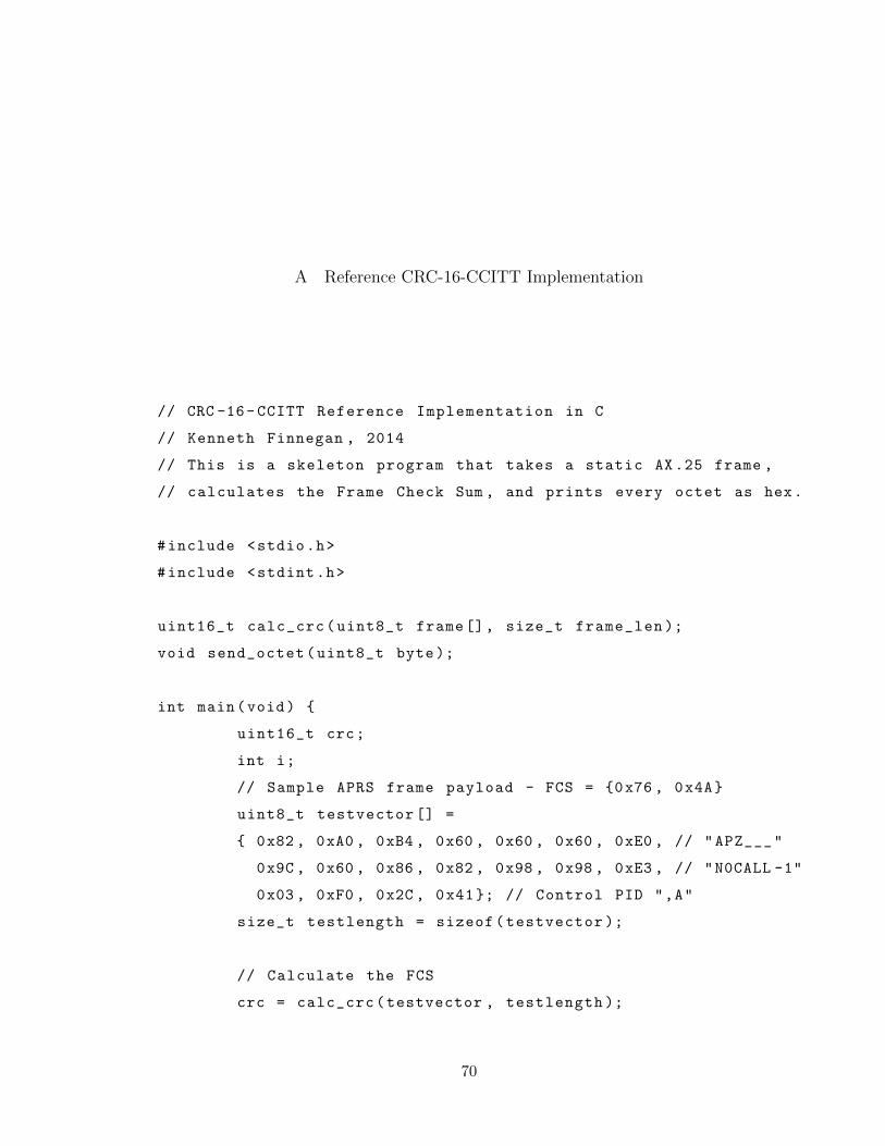
A Reference CRC-16-CCITT Implementation
// CRC -16-CCITT Reference Implementation in C
// Kenneth Finnegan , 2014
// This is a skeleton program that takes a static AX.25 frame ,
// calculates the Frame Check Sum , and prints every octet as hex.
#include <stdio.h>
#include <stdint.h>
uint16_t calc_crc(uint8_t frame[], size_t frame_len );
void send_octet(uint8_t byte);
int main(void) {
uint16_t crc;
int i;
// Sample APRS frame payload - FCS = {0x76 , 0x4A}
uint8_t testvector [] =
{ 0x82 , 0xA0 , 0xB4 , 0x60 , 0x60 , 0x60 , 0xE0 , // "APZ___"
0x9C , 0x60 , 0x86 , 0x82 , 0x98 , 0x98 , 0xE3 , // "N0CALL -1"
0x03 , 0xF0 , 0x2C , 0x41}; // Control PID ",A"
size_t testlength = sizeof(testvector );
// Calculate the FCS
crc = calc_crc(testvector , testlength );
70
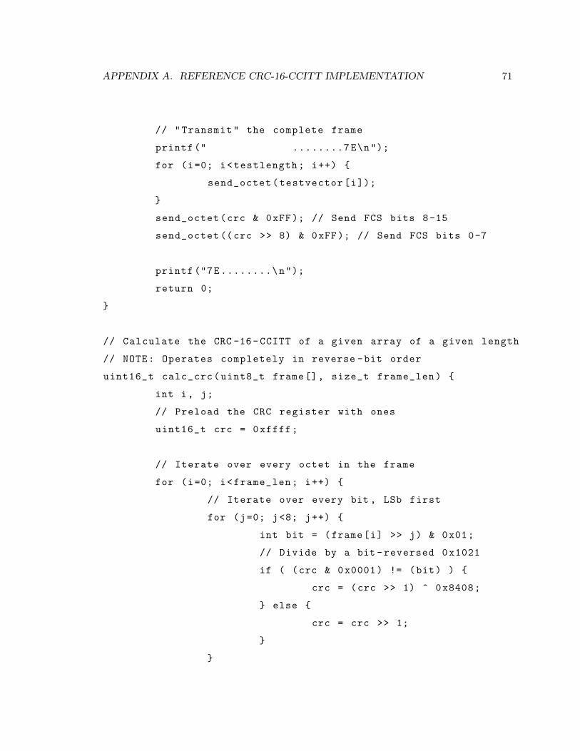
APPENDIX A. REFERENCE CRC-16-CCITT IMPLEMENTATION 71
// "Transmit" the complete frame
printf (" ........7E\n");
for (i=0; i<testlength; i++) {
send_octet(testvector[i]);
}
send_octet(crc & 0xFF); // Send FCS bits 8-15
send_octet ((crc >> 8) & 0xFF); // Send FCS bits 0-7
printf ("7E........\n");
return 0;
}
// Calculate the CRC -16- CCITT of a given array of a given length
// NOTE: Operates completely in reverse -bit order
uint16_t calc_crc(uint8_t frame[], size_t frame_len) {
int i, j;
// Preload the CRC register with ones
uint16_t crc = 0xffff;
// Iterate over every octet in the frame
for (i=0; i<frame_len; i++) {
// Iterate over every bit , LSb first
for (j=0; j<8; j++) {
int bit = (frame[i] >> j) & 0x01;
// Divide by a bit -reversed 0x1021
if ( (crc & 0x0001) != (bit) ) {
crc = (crc >> 1) ^ 0x8408;
} else {
crc = crc >> 1;
}
}
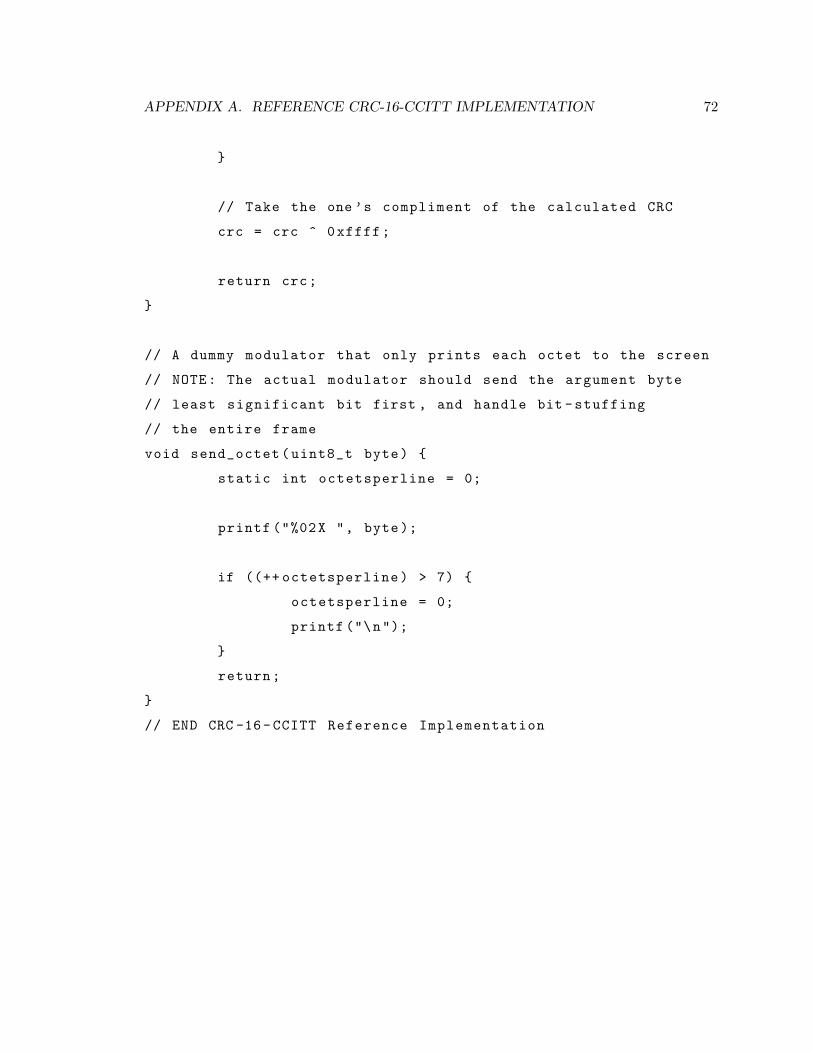
APPENDIX A. REFERENCE CRC-16-CCITT IMPLEMENTATION 72
}
// Take the one ’s compliment of the calculated CRC
crc = crc ^ 0xffff;
return crc;
}
// A dummy modulator that only prints each octet to the screen
// NOTE: The actual modulator should send the argument byte
// least significant bit first , and handle bit -stuffing
// the entire frame
void send_octet(uint8_t byte) {
static int octetsperline = 0;
printf ("%02X ", byte);
if ((++ octetsperline) > 7) {
octetsperline = 0;
printf ("\n");
}
return;
}
// END CRC -16-CCITT Reference Implementation
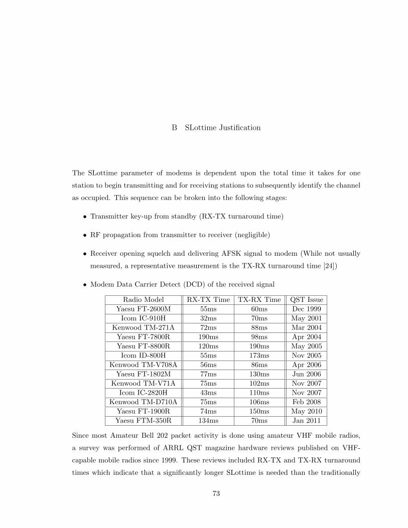
B SLottime Justification
The SLottime parameter of modems is dependent upon the total time it takes for one
station to begin transmitting and for receiving stations to subsequently identify the channel
as occupied. This sequence can be broken into the following stages:
• Transmitter key-up from standby (RX-TX turnaround time)
• RF propagation from transmitter to receiver (negligible)
• Receiver opening squelch and delivering AFSK signal to modem (While not usually
measured, a representative measurement is the TX-RX turnaround time [24])
• Modem Data Carrier Detect (DCD) of the received signal
Radio Model RX-TX Time TX-RX Time QST Issue
Yaesu FT-2600M 55ms 60ms Dec 1999
Icom IC-910H 32ms 70ms May 2001
Kenwood TM-271A 72ms 88ms Mar 2004
Yaesu FT-7800R 190ms 98ms Apr 2004
Yaesu FT-8800R 120ms 190ms May 2005
Icom ID-800H 55ms 173ms Nov 2005
Kenwood TM-V708A 56ms 86ms Apr 2006
Yaesu FT-1802M 77ms 130ms Jun 2006
Kenwood TM-V71A 75ms 102ms Nov 2007
Icom IC-2820H 43ms 110ms Nov 2007
Kenwood TM-D710A 75ms 106ms Feb 2008
Yaesu FT-1900R 74ms 150ms May 2010
Yaesu FTM-350R 134ms 70ms Jan 2011
Since most Amateur Bell 202 packet activity is done using amateur VHF mobile radios,
a survey was performed of ARRL QST magazine hardware reviews published on VHF-
capable mobile radios since 1999. These reviews included RX-TX and TX-RX turnaround
times which indicate that a significantly longer SLottime is needed than the traditionally
73

APPENDIX B. SLOTTIME JUSTIFICATION 74
suggested 100ms. This is due to none of the evaluated radios being fast enough to key up,
a second radio to open squelch, and then allow any time for modem DCD before the end
of a slot.
The author suggests that a new default of 300ms SLottime be considered. This value allows
many more radios to be able to detect a transmission in progress before the expiration of
the slot time, based on the values collected above.