Embed Size (px)
Citation preview

Examine Construct Validity of Computerized Adaptive Test in K-12 Assessments
Shudong Wang
NWEA
Hong Jiao
University of Maryland
The modified version of this paper will be presented at the annual meeting of the National
Council on Measurement in Education. April 12-16, 2012, Vancouver, British Columbia.
Send correspondence to:
Shudong Wang
Northwest Evaluation Association (NWEA)
121 NW Everett St.
Portland, OR 97206

1
ABSTRACT
The purpose of this study is to investigate the effect of missing data in computerized
adaptive tests (CAT) on test construct validity. The CAT method is now becoming more
popular in educational assessment. However, conducting construct validity on CAT data has
unique challenges for researchers because of the nature of missing data in the CAT. Unlike linear
tests in which missing mechanisms that is defined as missing type can be regarded as missing at
random, the CAT algorithm determines that missing CAT is not random. The study using
simulation methods examined the effect of different missing data generated from different IRT
models on recovery of internal structure of tests at both item and item cluster levels. Results
show it is impossible to recover the CAT test internal structure by using items as observable
variables, but by parceling items and using parcels as observable variables, the test internal
structure can be recovered. Parceling has the effect of over fitting models.
2
INTRODUCTION
Student achievement as measured in K-12 achievement tests is an abstract attribute. The
construct of achievement is theoretically defined and operationalized by a test. The construct of a
test is a theoretical representation of the underlying traits, concepts, attributes, processes, or
structures the test is designed to measure and directly relates to test validity (Cronbach, 1971;
Messick, 1989). The validity of a test is the extent to which it is designed to measure, and
according to the Standards for Educational and Psychological Testing (American Educational
Research Association [AERA], American Psychological Association [APA], & National Council
on Measurement in Education [NCME], 1999), validity is the most important consideration in
test development and evaluation. Five sources of validity evidence specified in the Standards
include: (a) test content, (b) response process, (c) internal structure, (d) relations to other
variables, and (e) consequences of testing. The test validation process in K-12 assessments relies
heavily on content validation procedures (Kane, 2006; Lissitz & Samuelsen, 2007), but it
shouldn’t diminish the need for multiple sources of evidence to establish internal test meaning,
including theoretical components, even for educational tests (Embretson, 2007). Any source of
validity evidence should be viewed as supporting a specific interpretation or use of test scores.
Currently in K-12 education, most state tests and large-scale standardized assessment
programs provide all or part of five sources of validity evidence for the interpretation of
achievement test results in their test technical manuals. Different statistical techniques have been
used to provide evidence to establish valid inference. Because confirmatory factor analysis
(CFA) deals with relationships among sets of underlying latent variables and a larger number of
observable indicators at either item or item cluster levels, CFA is currently the most frequently
used method to provide evidence on the internal structure of a test and addresses the question of
whether the items or subtests measure the hypothesized latent variable(s). However, applying the
CFA method to investigate internal structure of tests has two major practical challenges: using
categorical observable variables and missing data.
For the first challenge, the choice of the level of an indicator in general factor analysis,
has a significant effect on evaluating the construct. For example, the choice of item level
indicators or item cluster/parcel indicators that sum or average item scores as observable
variables in the CFA could impact model evaluation result (Bandalos, 2002; Bandalos & Finney,
2001; Hall, Snell & Foust, 1999; Little, Cunningham, Shahar & Widaman, 2002; Nasser &
Wisenbaker, 2003). Most item level variables used in K-12 assessment are categorical variables
that are binary/dichotomous responses from multiple-choice or griddable items, and polytomous
responses from constructed response items, performance events, or innovative items. Through
the use of item parcels/clusters/testlets, sub-tests level variables can be assumed to be continuous
observable variables and also be used as such in most current practices. However, some
psychometric concerns (Bandalos & Finney, 2001; Bollen &Lennox, 1991; Coanders, Satorra, &
Saris, 1997; Hall, Snell, & Foust, 1999; Marsh & O’Neill, 1984; Shevlin, Miles, & Bunting,
1997) over item parceling include: (a) loss of information about the relative importance of
individual items, (b) parceling of ordinal scales with undefined values, (c) limited range of latent
variables and biased variance and covariance parameters, and (d) underestimate the relationships
of latent variable due to limited reliability of the scale. When the sample size is small, the
benefits of using parcels over items as observable indicators (Bandalos, 2002; Bandalos &
Finney, 2001; Bentler, 2009; Cattell, 1974; Hau & Marsh, 2004; Marsh, Hau, Balla, & Grayson,
1998; Nasser & Wisenbaker, 2003; West, Finch, & Curran, 1995; Yang & Green, 2010a) include:

3
(a) having fewer free parameters to be estimated compared to the number of observations and
improves model fit, (b) reducing the problems of non-normality, (c) not requiring data
transformation, and (d) robust normal theory estimation, or distribution-free estimation.
However, these benefits will diminish when items are unidimensional or have high item
communalities, and sample sizes are large.
One interesting issue is that the effect of parceling on estimates of factor analysis
parameters closely relates to the choice of item response theory (IRT) models that most large
scale programs use to score, equate, and scale the tests. The IRT models can be equivalent to
item factor analysis (IFA) within latent variable modeling framework (McDonald, 1999, 2000;
Muthen & Asparouhov, 2002; Muthén & Muthén, 2006). The IFA model is factor analysis that
uses items as observable variables. Instead of modeling the linear relationship between indictors
and latent variable(s) as is done in CFA, nonlinear relationships between items and the latent
variable set are modeled through link functions that link latent variables to categorical
observable variables. The IFA with equal discrimination functions or factor loadings is
equivalent to the Rasch model (Rasch, 1960) or the one-parameter IRT model (Hambleton &
Swaminathan, 1985), in which item discrimination parameters are constant. Other dichotomous
IRT models, such 2-parameter and 3-parameter IRT models, can model items with different
discrimination parameters, which is equivalent to IFA with non-equal equal discrimination
functions or factor loadings. Studies on the parceling effect on nonlinear factor analysis with
non-equal discrimination functions or factor loadings conditions are very limited (Ferrando,
2009). Most studies on the parceling effect consider only the parceling of continuous indicators
that have equal discrimination functions or factor loadings and under these conditions. It is not
surprising that parceling has little impact on the relationship between indicators and latent
variables (Alhija & Wisenbaker, 2006; Bandolas, 2002; Hau & Marsh, 2004) in linear cases.
Overall, parceling items is currently a commonly used technique based upon theoretical
rationales.
The second challenge of using CFA to conduct construct validity analysis is missing data.
The reasons missing data exists in educational assessments are numerous; some reasons include:
(1) student behaviors, such as students motivation, failing to attend, unwilling to answer,
cheating in taking a test; (2) scoring, such as scoring mistakes; and (3) administration and
operation, such as lost test booklets, scanning mistakes, bad weather, fire alarm. Other reasons
are due to test design, such as the choice of linear tests vs. computerized adaptive tests (CAT).
According to Rubin’s (1976) missing data mechanisms, educational data can be classified as
missing completely at random (MCAR), missing at random (MAR), or missing not at random
(MNAR). Within the latent variable modeling framework (Muthén, Asparouhov, Hunter, &
Leuchter, 2011), if missingness is related to observed variables, then it can be MAR; if
missingness is related to latent variables, such as student achievement ability, then it is MNAR
and such missing data refer to non-ignorable missing data. The focus of this paper is on data
missing due to test design, i.e., missing data in CAT. Because a CAT operates on an algorithm
that selects items from an item bank to match a student’s provisional ability estimate, each
student test event contains responses to a small subset of the item pool. Two additional features
of CAT data compared to linear test data are: (1) restricted range of person ability for given
items and (2) persons with different ability get different items. If a whole item bank is imagined
as a linear test, then missingness in a CAT can be taken as due to item responses missing from
the collection of test sessions. For example, for Reading and Mathematics of Measure of
Academic Progress (MAP, NWEA, 2011) tests, typical missing rates are around 98% because

4
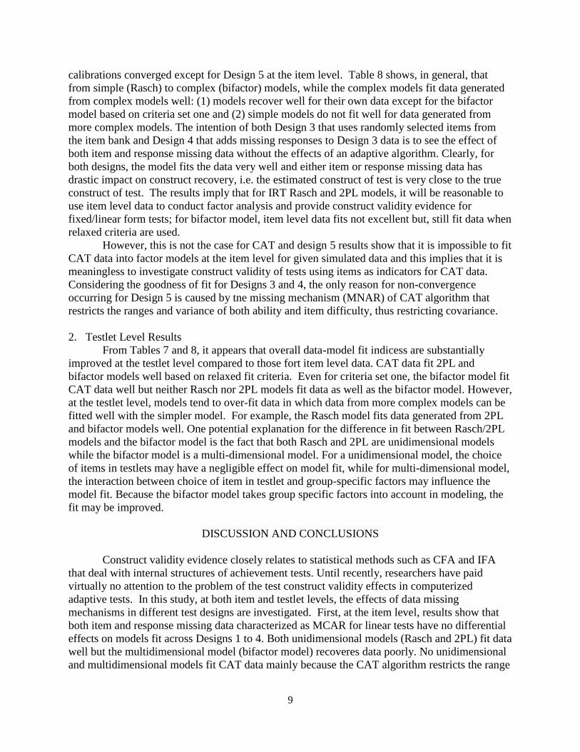
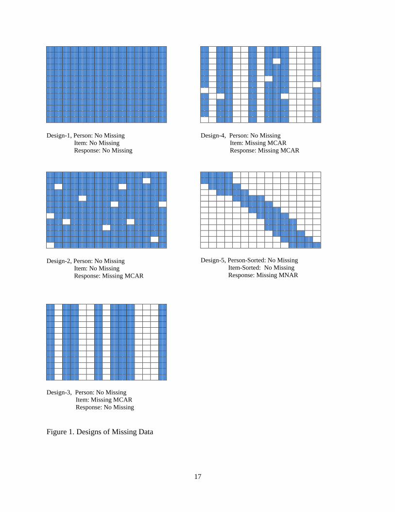
the ratio of item pool size to test length is around 50 and data are very sparse. Figure 1 illustrates
five missing designs. For simplification, all designs assume there is no person missing data.
Design 1 as the baseline design shows no missing on item and response, and Design 2 shows
missing on the response. Both Designs 1 and 2 represent responses from linear tests shown in
Tables 1 and 2. Design 3 and 4 represent neither linear nor CAT cases exactly because there will
be no missing item responses in linear tests and some persons will answer some items in CATs.
These two designs reflect the fact that observable indicators are not complete and are sampled
from the existing pool of observable indicators according to content requirements in most CAT
situations. The difference between Design 3 and 4 is that Design 4 contains additional missing
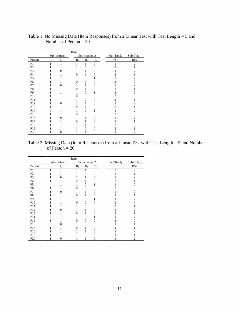
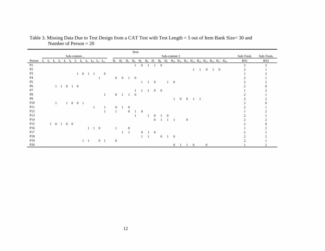
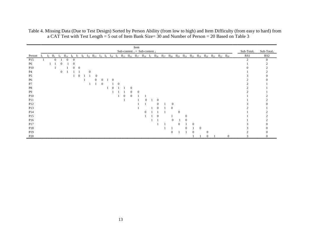
responses. Tables 3 and 4 show the data pattern for CAT as Design 5. Besides the missing rate
attributed to the CAT algorithm, restricting ability range in data also has an impact on factor
analysis because of the restricted of range of observation variables.
Nowadays, CAT is becoming more popular in educational assessment. Right now,
Oregon, Delaware, and Idaho use CAT in their state assessments, and several other states
(Georgia, Hawaii, Maryland, North Carolina, South Dakota, Utah, and Virginia) are in various
stages of CAT development. As a matter of fact, one of the two consortia was created as part of
the Race to the Top initiative. The SMARTER Balanced Assessment Consortium (SBAC),
consisting of over half of the states, is committed to a computerized adaptive model because it
represents a unique opportunity to create a large-scale assessment system that provides
maximally accurate achievement results for each student (Race to the Top Assessment Program,
2010). There is an urgent need to gain understanding about assessing construct validity in a CAT
in real operation. The purpose of this study is to investigate the effect of missing data in CAT on
construct validity of a test.
METHOD
Almost all large-scale standardized K-12 testing programs use an IRT model in scoring,
equating, and scaling. The internal structure of a test is often reported as the evidence related to
construct validity based on factor analysis. Some test programs report the internal structure using
items as observable indicators or variables in factor analysis, others use item testlets or parcels as
observable indicators or variables in factor analysis, and some other reports use both. The
theoretical framework of this study is to use a unifying approach that combines both linear and
non-liner factor analyses so that the impact of missing data on factor structure of a test can be
compared at both item and item parcel/testlet levels. The linear factor analysis models the
relationship between latent variables and continuous observable variables. While nonlinear factor
analysis models relationships among latent variables and categorical observable variables, the
IRT model can be considered as a special case of nonlinear factor analysis.
1. Factor Model
1.1 Continuous observed variables
Confirmatory factor analysis (CFA) that describes the covariance among observed
variables as a function of latent factors makes some assumptions. These assumptions include that
unique factors are normally distributed or independent with normally distributed residuals,
manifest indictors are continuous and conditionally normal distributed, and there is a linear
relationship between observed and latent factors. When sub-content or goal scores from tests are
used as manifest indictors, the distribution properties usually meet these assumptions. Let yij
5
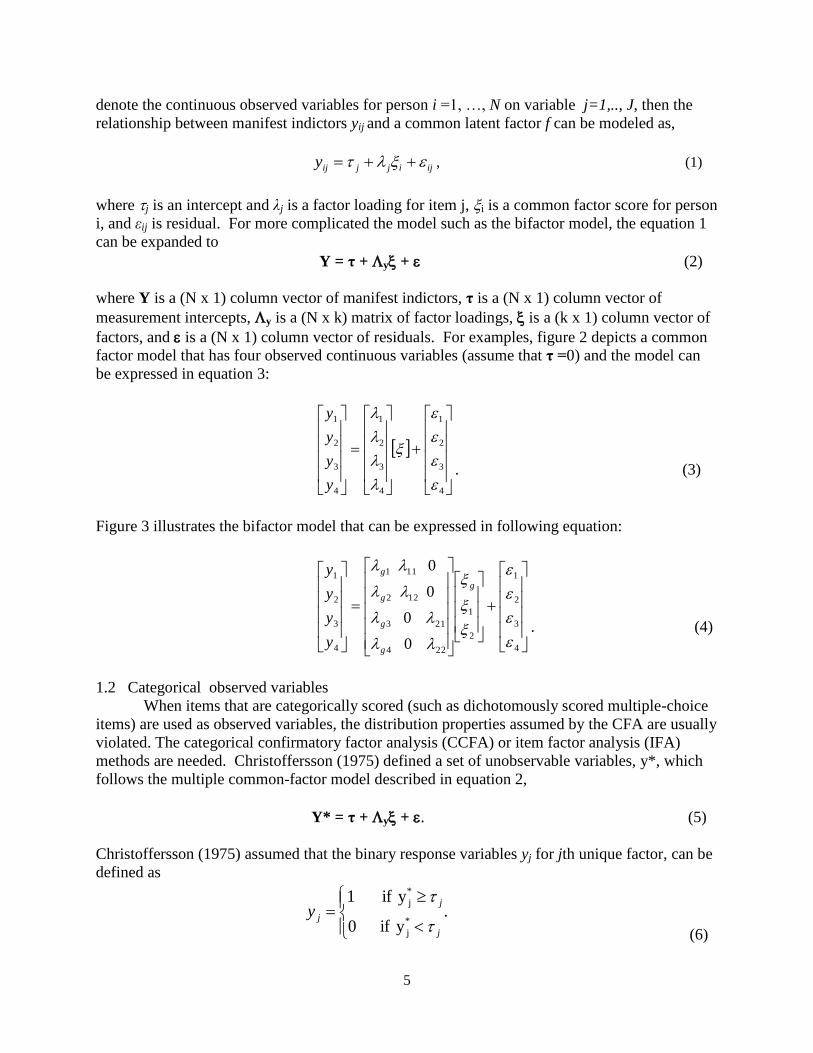
denote the continuous observed variables for person i =1, …, N on variable j=1,.., J, then the
relationship between manifest indictors yij and a common latent factor f can be modeled as,
ijijjijy , (1)
where j is an intercept and lj is a factor loading for item j, i is a common factor score for person
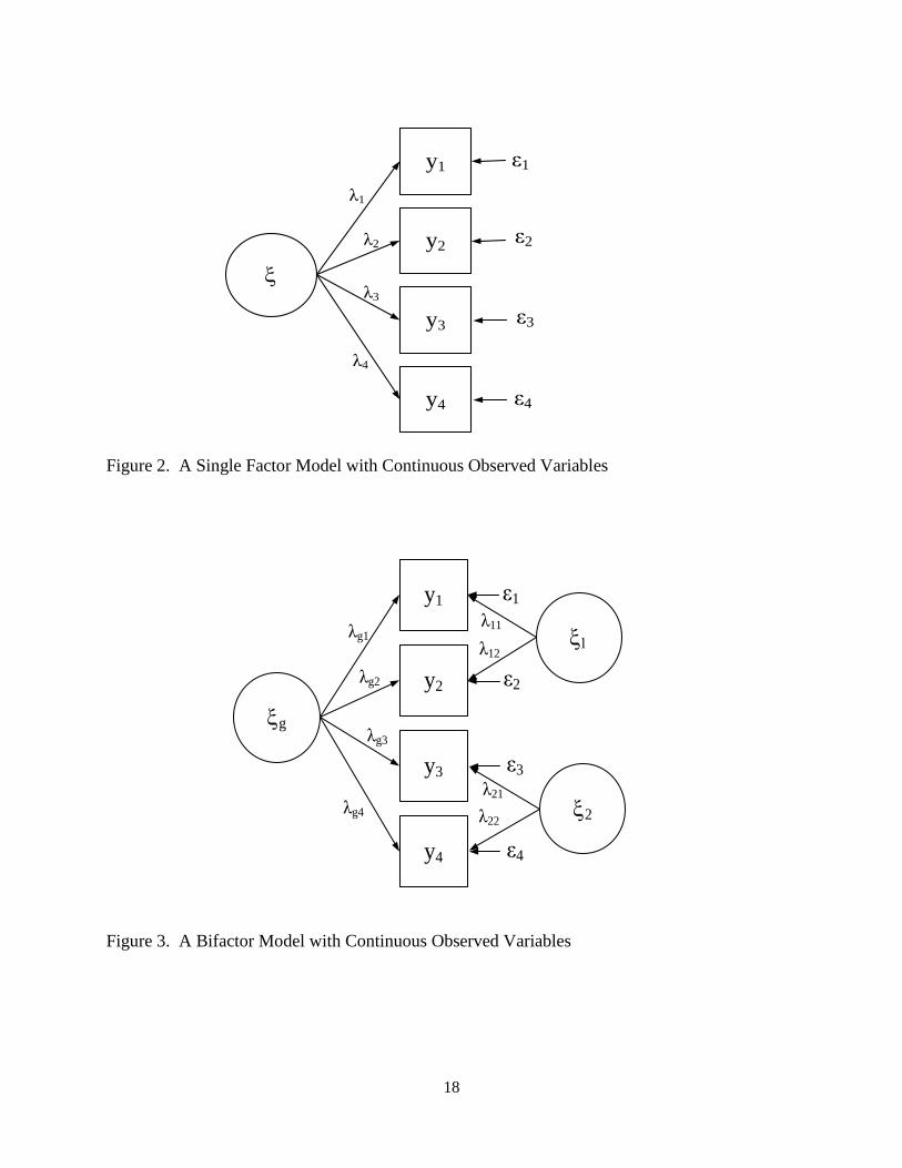
i, and eij is residual. For more complicated the model such as the bifactor model, the equation 1
can be expanded to
Y = t + y + (2)
where Y is a (N x 1) column vector of manifest indictors, t is a (N x 1) column vector of
measurement intercepts, y is a (N x k) matrix of factor loadings, is a (k x 1) column vector of
factors, and is a (N x 1) column vector of residuals. For examples, figure 2 depicts a common
factor model that has four observed continuous variables (assume that t =0) and the model can
be expressed in equation 3:
4
3
2
1
4
3
2
1
4
3
2
1
y
y
y
y
. (3)
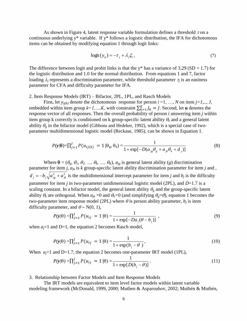
Figure 3 illustrates the bifactor model that can be expressed in following equation:
4
3
2
1
2
1
224
213
122
111
4
3
2
1
0
0
0
0
g
g
g
g
g
y
y
y
y
. (4)
1.2 Categorical observed variables
When items that are categorically scored (such as dichotomously scored multiple-choice
items) are used as observed variables, the distribution properties assumed by the CFA are usually
violated. The categorical confirmatory factor analysis (CCFA) or item factor analysis (IFA)
methods are needed. Christoffersson (1975) defined a set of unobservable variables, y*, which
follows the multiple common-factor model described in equation 2,
Y* = t + y + . (5)
Christoffersson (1975) assumed that the binary response variables yj for jth unique factor, can be
defined as
. yif 0
yif 1
*
j
*
j
j
j
jy
(6)
6
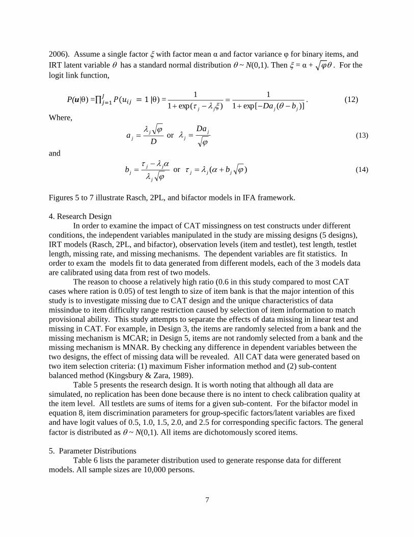
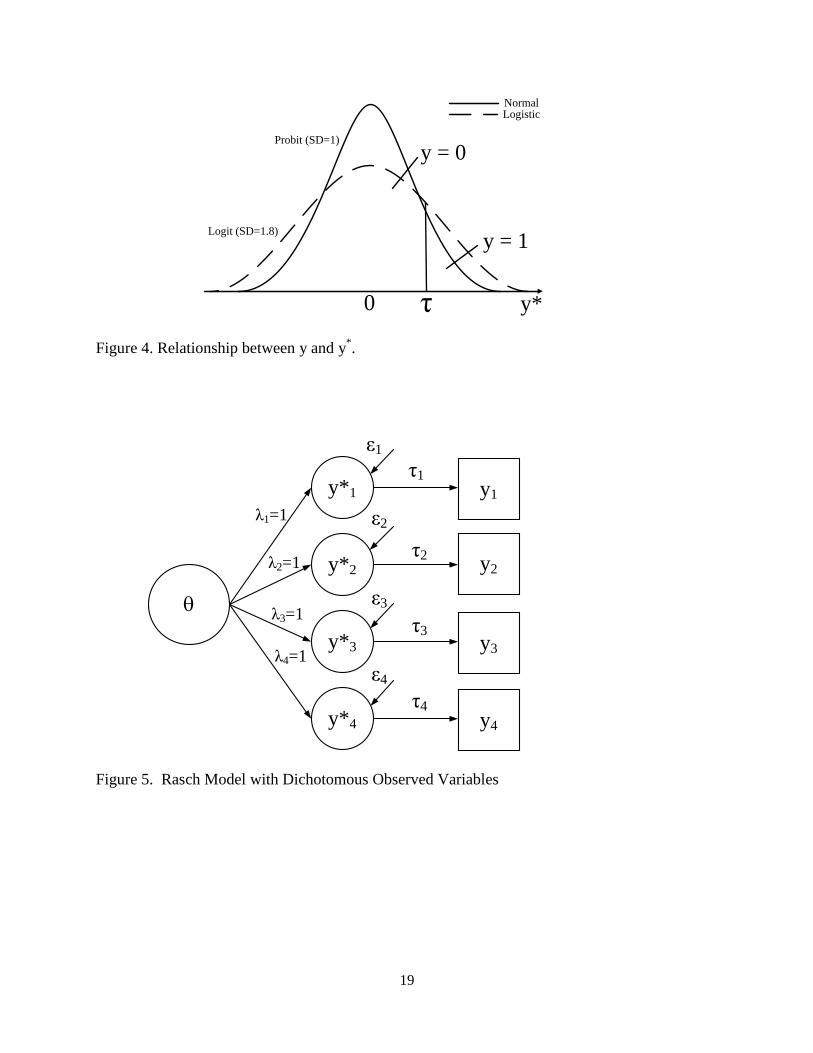
As shown in Figure 4, latent response variable formulation defines a threshold on a
continuous underlying y* variable. If y* follows a logistic distribution, the IFA for dichotomous
items can be obtained by modifying equation 1 through logit links:
ijjijy )(logit , (7)
The difference between logit and probit links is that the y* has a variance of 3.29 (SD = 1.7) for
the logistic distribution and 1.0 for the normal distribution. From equations 1 and 7, factor
loading j represents a discrimination parameter, while threshold parameter j is an easiness
parameter for CFA and difficulty parameter for IFA.
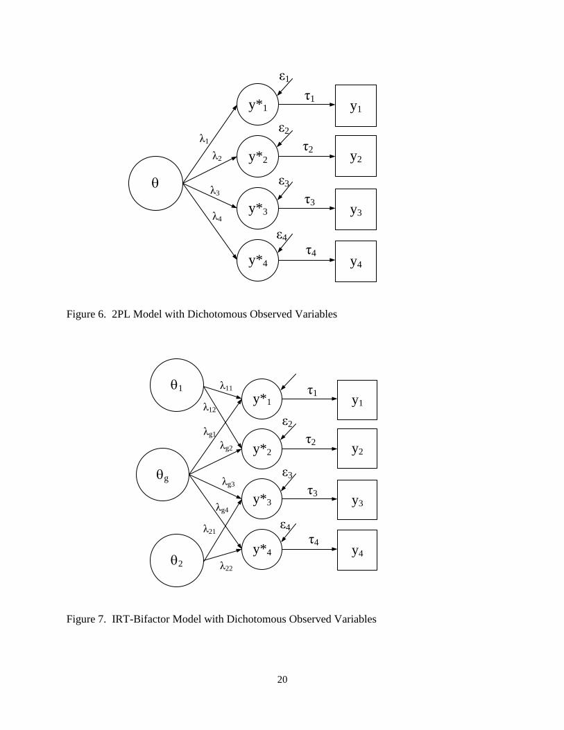
2. Item Response Models (IRT) – Bifactor, 2PL, 1PL, and Rasch Models
First, let yij(k) denote the dichotomous response for person i =1, …, N on item j=1,.., J,
embedded within item group k=1,…,K, with constraint ∑ . Second, let u denotes the
response vector of all responses. Then the overall probability of person i answering item j within
item group k correctly is conditioned on k group-specific latent ability k and a general latent
ability g in the bifactor model (Gibbons and Hedeker, 1992), which is a special case of two-
parameter multidimensional logistic model (Reckase, 1985), can be shown in Equation 1.
P(y|)=∏ g, k) =
)](exp[1
1
jkjkgjg daaD (8)
Where = (g, 1, 2, …, k, …, K), ajg is general latent ability (g) discrimination
parameter for item j, ajk is k group-specific latent ability discrimination parameter for item j and ,
22
jkjgjj aabd is the multidimensional intercept parameter for item j and bj is the difficulty
parameter for item j in two-parameter unidimensional logistic model (2PL), and D=1.7 is a
scaling constant. In a bifactor model, the general latent ability g and the group-specific latent
ability k are orthogonal. When ajk =0 and k=0 (and simplifying g=), equation 1 becomes the
two-parameter item response model (2PL) where is person ability parameter, bj is item
difficulty parameter, and N(0, 1),
P(y|) =∏ ) =
)](exp[1
1
jj bDa , (9)
when aj=1 and D=1, the equation 2 becomes Rasch model,
P(y|) =∏ ) =
)exp(1
1
jb, (10)
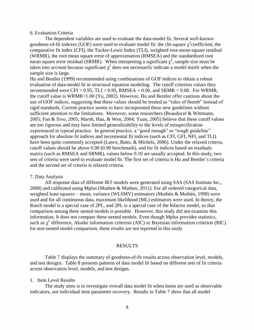
When aj=1 and D=1.7, the equation 2 becomes one-parameter IRT model (1PL),
P(y|) =∏ ) =
)](exp[1
1
jbD. (11)
3. Relationship between Factor Models and Item Response Models
The IRT models are equivalent to item level factor models within latent variable
modeling framework (McDonald, 1999, 2000; Muthen & Asparouhov, 2002; Muthén & Muthén,
7
2006). Assume a single factor with factor mean a and factor variance f for binary items, and
IRT latent variable has a standard normal distribution ~ N(0,1). Then = a + √ . For the
logit link function,
P(u|) =∏ ) =
)](exp[1
1
)exp(1
1
jjjj bDa
. (12)
Where,
D
aj
j
or
j
j
Da (13)
and
j
jj
jb
or )( jjj b (14)
Figures 5 to 7 illustrate Rasch, 2PL, and bifactor models in IFA framework.
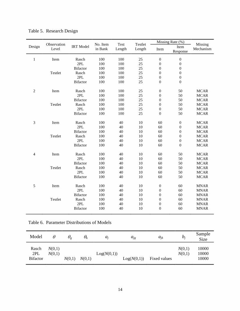
4. Research Design
In order to examine the impact of CAT missingness on test constructs under different
conditions, the independent variables manipulated in the study are missing designs (5 designs),
IRT models (Rasch, 2PL, and bifactor), observation levels (item and testlet), test length, testlet
length, missing rate, and missing mechanisms. The dependent variables are fit statistics. In
order to exam the models fit to data generated from different models, each of the 3 models data
are calibrated using data from rest of two models.
The reason to choose a relatively high ratio (0.6 in this study compared to most CAT
cases where ration is 0.05) of test length to size of item bank is that the major intention of this
study is to investigate missing due to CAT design and the unique characteristics of data
missindue to item difficulty range restriction caused by selection of item information to match
provisional ability. This study attempts to separate the effects of data missing in linear test and
missing in CAT. For example, in Design 3, the items are randomly selected from a bank and the
missing mechanism is MCAR; in Design 5, items are not randomly selected from a bank and the
missing mechanism is MNAR. By checking any difference in dependent variables between the
two designs, the effect of missing data will be revealed. All CAT data were generated based on
two item selection criteria: (1) maximum Fisher information method and (2) sub-content
balanced method (Kingsbury & Zara, 1989).
Table 5 presents the research design. It is worth noting that although all data are
simulated, no replication has been done because there is no intent to check calibration quality at
the item level. All testlets are sums of items for a given sub-content. For the bifactor model in
equation 8, item discrimination parameters for group-specific factors/latent variables are fixed
and have logit values of 0.5, 1.0, 1.5, 2.0, and 2.5 for corresponding specific factors. The general
factor is distributed as ~ N(0,1). All items are dichotomously scored items.
5. Parameter Distributions
Table 6 lists the parameter distribution used to generate response data for different
models. All sample sizes are 10,000 persons.
8
6. Evaluation Criteria
The dependent variables are used to evaluate the data-model fit. Several well-known
goodness-of-fit indexes (GOF) were used to evaluate model fit: the chi-square χ2coefficient, the
comparative fit index (CFI), the Tucker-Lewis Index (TLI), weighted root-mean-square residual
(WRMR), the root mean square error of approximation (RMSEA) and the standardized root
mean square error residual (SRMR). When interpreting a significant χ2, sample size must be
taken into account because significant χ2 does not necessarily indicate a model misfit when the
sample size is large.
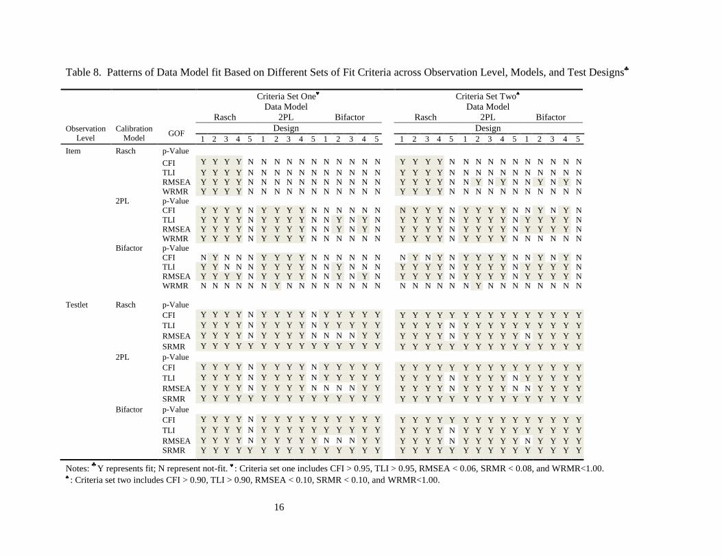
Hu and Bentler (1999) recommended using combinations of GOF indices to obtain a robust
evaluation of data-model fit in structural equation modeling. The cutoff criterion values they
recommended were CFI > 0.95, TLI > 0.95, RMSEA < 0.06, and SRMR < 0.08. For WRMR,
the cutoff value is WRMR<1.00 (Yu, 2002). However, Hu and Bentler offer cautions about the
use of GOF indices, suggesting that these values should be treated as “rules of thumb” instead of
rigid standards. Current practice seems to have incorporated these new guidelines without
sufficient attention to the limitations. Moreover, some researchers (Beauducel & Wittmann,
2005; Fan & Sivo, 2005; Marsh, Hau, & Wen, 2004; Yuan, 2005) believe that these cutoff values
are too rigorous and may have limited generalizability to the levels of misspecification
experienced in typical practice. In general practice, a “good enough” or “rough guideline”
approach for absolute fit indices and incremental fit indices (such as CFI, GFI, NFI, and TLI)
have been quite commonly accepted (Lance, Butts, & Michels, 2006). Under the relaxed criteria,
cutoff values should be above 0.90 (0.90 benchmark), and for fit indices based on residuals
matrix (such as RMSEA and SRMR), values below 0.10 are usually accepted. In this study, two
sets of criteria were used to evaluate model fit. The first set of criteria is Hu and Bentler’s criteria
and the second set of criteria is relaxed criteria.
7. Data Analysis
All response data of different IRT models were generated using SAS (SAS Institute Inc.,
2008) and calibrated using Mplus (Muthen & Muthen, 2011). For all ordered categorical data,
weighted least squares – mean, variance (WLSMV) estimators (Muthén & Muthén, 1998) were
used and for all continuous data, maximum likelihood (ML) estimators were used. In theory, the
Rasch model is a special case of 2PL, and 2PL is a special case of the bifactor model, so that
comparison among three nested models is possible. However, this study did not examine this
information. It does not compare these nested models. Even though Mplus provides statistics,
such as χ2 difference, Akaike information criterion (AIC) or Bayesian information criterion (BIC)
for non-nested model comparison, these results are not reported in this study
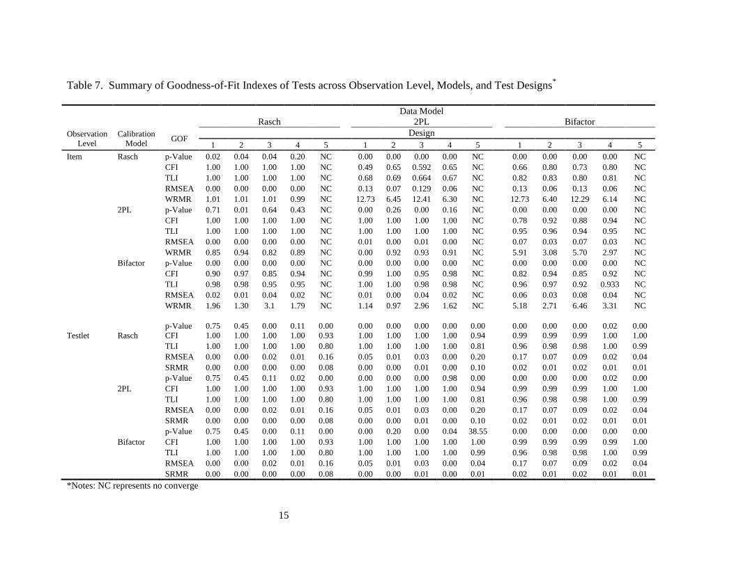
RESULTS
Table 7 displays the summary of goodness-of-fit results across observation level, models,
and test designs. Table 8 presents patterns of data model fit based on different sets of fit criteria
across observation level, models, and test designs.
1. Item Level Results
The study aims is to investigate overall data model fit when items are used as observable
indicators, not individual item parameter recovery. Results in Table 7 show that all model
9
calibrations converged except for Design 5 at the item level. Table 8 shows, in general, that
from simple (Rasch) to complex (bifactor) models, while the complex models fit data generated
from complex models well: (1) models recover well for their own data except for the bifactor
model based on criteria set one and (2) simple models do not fit well for data generated from
more complex models. The intention of both Design 3 that uses randomly selected items from
the item bank and Design 4 that adds missing responses to Design 3 data is to see the effect of
both item and response missing data without the effects of an adaptive algorithm. Clearly, for
both designs, the model fits the data very well and either item or response missing data has
drastic impact on construct recovery, i.e. the estimated construct of test is very close to the true
construct of test. The results imply that for IRT Rasch and 2PL models, it will be reasonable to
use item level data to conduct factor analysis and provide construct validity evidence for
fixed/linear form tests; for bifactor model, item level data fits not excellent but, still fit data when
relaxed criteria are used.
However, this is not the case for CAT and design 5 results show that it is impossible to fit
CAT data into factor models at the item level for given simulated data and this implies that it is
meaningless to investigate construct validity of tests using items as indicators for CAT data.
Considering the goodness of fit for Designs 3 and 4, the only reason for non-convergence
occurring for Design 5 is caused by tne missing mechanism (MNAR) of CAT algorithm that
restricts the ranges and variance of both ability and item difficulty, thus restricting covariance.
2. Testlet Level Results
From Tables 7 and 8, it appears that overall data-model fit indicess are substantially
improved at the testlet level compared to those fort item level data. CAT data fit 2PL and
bifactor models well based on relaxed fit criteria. Even for criteria set one, the bifactor model fit
CAT data well but neither Rasch nor 2PL models fit data as well as the bifactor model. However,
at the testlet level, models tend to over-fit data in which data from more complex models can be
fitted well with the simpler model. For example, the Rasch model fits data generated from 2PL
and bifactor models well. One potential explanation for the difference in fit between Rasch/2PL
models and the bifactor model is the fact that both Rasch and 2PL are unidimensional models
while the bifactor model is a multi-dimensional model. For a unidimensional model, the choice
of items in testlets may have a negligible effect on model fit, while for multi-dimensional model,
the interaction between choice of item in testlet and group-specific factors may influence the
model fit. Because the bifactor model takes group specific factors into account in modeling, the
fit may be improved.
DISCUSSION AND CONCLUSIONS
Construct validity evidence closely relates to statistical methods such as CFA and IFA
that deal with internal structures of achievement tests. Until recently, researchers have paid
virtually no attention to the problem of the test construct validity effects in computerized
adaptive tests. In this study, at both item and testlet levels, the effects of data missing
mechanisms in different test designs are investigated. First, at the item level, results show that
both item and response missing data characterized as MCAR for linear tests have no differential
effects on models fit across Designs 1 to 4. Both unidimensional models (Rasch and 2PL) fit data
well but the multidimensional model (bifactor model) recoveres data poorly. No unidimensional
and multidimensional models fit CAT data mainly because the CAT algorithm restricts the range

10
of person ability and item difficulty. Our results suggest that it is impossible to recover the
construct of CAT at the item level across models–even though recovering of construct of linear
tests are reasonably good. Second, at the testlet level, we demonstrate that item parceling
substantially improve models fit. At least for criteria set one, constructs of CAT can be
recovered partially for unidimensional models (Rasch and 2PL) and fully for the
multidimensional model (bifactor model). For both sets of criteria, constructs of linear tests
under Design 1 to 4 can be well recovered. The study shows that parceling over-fits model.
Limitations of this study include: (1) small size of item bank and (2) replication. Because
of time intensive calibrating the item bank for all three models (290 hours per model per
condition if 250 items used), relatively small item bank size were chosen and this affects the
missing rate in CAT data. All data studied are based on only one replication which may affect
generalizability of conclusions. The future directions should include increasing the size of the
item bank and more replications under different simulation conditions.
11
Table 1. No Missing Data (Item Responses) from a Linear Test with Test Length = 5 and
Number of Person = 20
Item
Sub-content 1 Sub-content 2 Sub-Total1 Sub-Total2
Person I1 I2 II1 II2 II3 RS1 RS2
P1 1 1
1 1 0 2 2
P2 1 1
1 0 0 2 1 P3 1 0
1 1 0 1 2
P4 1 1
0 1 0 2 1
P5 1 1
1 0 1 2 2 P6 1 1
0 0 0 2 0
P7 1 0
1 1 0 1 2
P8 1 1
0 1 0 2 1 P9 1 1
1 0 1 2 2
P10 1 1
0 0 0 2 0
P11 1 1
1 0 0 2 1 P12 1 0
1 1 0 1 2
P13 1 1
0 1 0 2 1
P14 0 1
1 0 1 1 2 P15 1 1
0 0 0 2 0
P16 1 0
1 1 0 1 2
P17 1 1
0 1 0 2 1 P18 1 1
1 1 0 2 2
P19 1 1
1 0 0 2 1
P20 1 0 1 1 0 1 2
Table 2. Missing Data (Item Responses) from a Linear Test with Test Length = 5 and Number
of Person = 20
Item
Sub-content 1 Sub-content 2 Sub-Total1 Sub-Total2
Person I1 I2 II1 II2 II3 RS1 RS2
P1 1 1
1 1 0 2 2
P2 1 .
1 0 . 1 1 P3 1 0
1 1 0 1 2
P4 1 1
0 1 0 2 1
P5 . 1
1 0 1 1 2 P6 1 1
0 0 0 2 0
P7 1 0
1 1 0 1 2
P8 1 1
0 1 0 2 1 P9 1 .
1 . 1 1 2
P10 1 1
0 0 0 2 0
P11 1 1
1 0 . 2 1 P12 1 0
1 1 0 1 2
P13 1 1
0 1 0 2 1
P14 0 1
. 0 1 1 2 P15 1 1
0 0 0 2 0
P16 . 0
1 . 0 1 1 P17 1 1
0 1 0 2 1
P18 1 1
1 1 0 2 2
P19 1 .
1 0 0 1 1 P20 1 0 1 1 0 1 2
12
Table 3. Missing Data Due to Test Design from a CAT Test with Test Length = 5 out of Item Bank Size= 30 and
Number of Person = 20
Item
Sub-content 1 Sub-content 2 Sub-Total1 Sub-Total2
Person I1 I2 I3 I4 I5 I6 I7 I8 I9 I10 I11 I12 II1 II2 II3 II4 II5 II6 II7 II8 II9 II10 II11 II12 II13 II14 II15 II16 II17 II18 RS1 RS2
P1 1 0 1 1 0 2 2
P2
1 1 0 1 0 2 1
P3
1 0 1 1
0
1 2
P4
1
0 0 1 0
2 1
P5
1 1 0
1 0
2 2
P6
1 1 0 1 0
2 0
P7
1 1 1 0 0
1 2
P8
1 0 1 1 0
2 1
P9
1 0 0 1 1
2 2
P10
1
1 0 0 1
2 0
P11
1
1 0 1 0
2 1
P12
1 1
0 1 0
1 2
P13
1
1 0 1 0
2 1
P14
0 1 1 1
0
2 2
P15 1 0 1 0 0
2 0
P16
1 1 0
1
0
1 2
P17
1 1
0 1 0
2 1
P18
1 1
0 1 0
2 2
P19
1 1
0 1 0
2 1
P20 0 1 1 0 0 1 2
13
Table 4. Missing Data (Due to Test Design) Sorted by Person Ability (from low to high) and Item Difficulty (from easy to hard) from
a CAT Test with Test Length = 5 out of Item Bank Size= 30 and Number of Person = 20 Based on Table 3
Item
Sub-content 1 + Sub-content 2 Sub-Total1 Sub-Total2
Person I1 I2 II3 I4 II14 I6 I7 I8 I12 II13 I11 I9 I10 I5 II15 II16 II17 II18 I3 II26 II27 II28 II29 II24 II25 II19 II20 II21 II22 II30 RS1 RS2
P15 1
0 1 0 0
2 0
P6 1 1 0 1 0
1 2
P10
1
1 0 0
0 2
P4
0 1 1 1
0
1 2
P5
1 0 1 1 0
3 0
P6
1
0 0 1 0
2 0
P7
1 1 0
1 0
2 1
P8
1 0 1 1 0
2 1
P9
1 1 1 0 0
2 1
P10
1 0 0 1 1
1 2
P11
1
1 0 1 0
1 2
P12
1 1
0 1 0
3 0
P13
1
1 0 1 0
2 1
P14
0 1 1 1
0
1 2
P15
1 1 0
1
0
1 2
P16
1 1
0 1 0
1 2
P17
1 1
0 1 0
3 0
P18
1 1
0 1 0
3 0
P19
0 1 1 0
0
2 0
P20 1 1 0 1
0 3 0
14
Table 5. Research Design
Design Observation
Level IRT Model
No. Item
in Bank
Test
Length
Testlet
Length
Missing Rate (%) Missing
Mechanism Item Item
Response
1 Item Rasch 100 100 25 0 0
2PL 100 100 25 0 0
Bifactor 100 100 25 0 0
Testlet Rasch 100 100 25 0 0
2PL 100 100 25 0 0
Bifactor 100 100 25 0 0
2 Item Rasch 100 100 25 0 50 MCAR
2PL 100 100 25 0 50 MCAR
Bifactor 100 100 25 0 50 MCAR
Testlet Rasch 100 100 25 0 50 MCAR
2PL 100 100 25 0 50 MCAR
Bifactor 100 100 25 0 50 MCAR
3 Item Rasch 100 40 10 60 0 MCAR
2PL 100 40 10 60 0 MCAR
Bifactor 100 40 10 60 0 MCAR
Testlet Rasch 100 40 10 60 0 MCAR
2PL 100 40 10 60 0 MCAR
Bifactor 100 40 10 60 0 MCAR
4 Item Rasch 100 40 10 60 50 MCAR
2PL 100 40 10 60 50 MCAR
Bifactor 100 40 10 60 50 MCAR
Testlet Rasch 100 40 10 60 50 MCAR
2PL 100 40 10 60 50 MCAR
Bifactor 100 40 10 60 50 MCAR
5 Item Rasch 100 40 10 0 60 MNAR
2PL 100 40 10 0 60 MNAR
Bifactor 100 40 10 0 60 MNAR
Testlet Rasch 100 40 10 0 60 MNAR
2PL 100 40 10 0 60 MNAR
Bifactor 100 40 10 0 60 MNAR
Table 6. Parameter Distributions of Models
Model g k aj ajg ajk bj Sample
Size
Rasch N(0,1) N(0,1) 10000
2PL N(0,1) Log(N(0,1)) N(0,1) 10000
Bifactor N(0,1) N(0,1) Log(N(0,1)) Fixed values 10000
15
Table 7. Summary of Goodness-of-Fit Indexes of Tests across Observation Level, Models, and Test Designs*
Data Model
Rasch 2PL Bifactor
Observation
Level Calibration
Model GOF
Design
1 2 3 4 5 1 2 3 4 5 1 2 3 4 5
Item Rasch p-Value 0.02 0.04 0.04 0.20 NC 0.00 0.00 0.00 0.00 NC 0.00 0.00 0.00 0.00 NC
CFI 1.00 1.00 1.00 1.00 NC 0.49 0.65 0.592 0.65 NC 0.66 0.80 0.73 0.80 NC
TLI 1.00 1.00 1.00 1.00 NC 0.68 0.69 0.664 0.67 NC 0.82 0.83 0.80 0.81 NC
RMSEA 0.00 0.00 0.00 0.00 NC 0.13 0.07 0.129 0.06 NC 0.13 0.06 0.13 0.06 NC
WRMR 1.01 1.01 1.01 0.99 NC 12.73 6.45 12.41 6.30 NC 12.73 6.40 12.29 6.14 NC
2PL p-Value 0.71 0.01 0.64 0.43 NC 0.00 0.26 0.00 0.16 NC 0.00 0.00 0.00 0.00 NC
CFI 1.00 1.00 1.00 1.00 NC 1.00 1.00 1.00 1.00 NC 0.78 0.92 0.88 0.94 NC
TLI 1.00 1.00 1.00 1.00 NC 1.00 1.00 1.00 1.00 NC 0.95 0.96 0.94 0.95 NC
RMSEA 0.00 0.00 0.00 0.00 NC 0.01 0.00 0.01 0.00 NC 0.07 0.03 0.07 0.03 NC
WRMR 0.85 0.94 0.82 0.89 NC 0.00 0.92 0.93 0.91 NC 5.91 3.08 5.70 2.97 NC
Bifactor p-Value 0.00 0.00 0.00 0.00 NC 0.00 0.00 0.00 0.00 NC 0.00 0.00 0.00 0.00 NC
CFI 0.90 0.97 0.85 0.94 NC 0.99 1.00 0.95 0.98 NC 0.82 0.94 0.85 0.92 NC
TLI 0.98 0.98 0.95 0.95 NC 1.00 1.00 0.98 0.98 NC 0.96 0.97 0.92 0.933 NC
RMSEA 0.02 0.01 0.04 0.02 NC 0.01 0.00 0.04 0.02 NC 0.06 0.03 0.08 0.04 NC
WRMR 1.96 1.30 3.1 1.79 NC 1.14 0.97 2.96 1.62 NC 5.18 2.71 6.46 3.31 NC
p-Value 0.75 0.45 0.00 0.11 0.00 0.00 0.00 0.00 0.00 0.00 0.00 0.00 0.00 0.02 0.00
Testlet Rasch CFI 1.00 1.00 1.00 1.00 0.93 1.00 1.00 1.00 1.00 0.94 0.99 0.99 0.99 1.00 1.00
TLI 1.00 1.00 1.00 1.00 0.80 1.00 1.00 1.00 1.00 0.81 0.96 0.98 0.98 1.00 0.99
RMSEA 0.00 0.00 0.02 0.01 0.16 0.05 0.01 0.03 0.00 0.20 0.17 0.07 0.09 0.02 0.04
SRMR 0.00 0.00 0.00 0.00 0.08 0.00 0.00 0.01 0.00 0.10 0.02 0.01 0.02 0.01 0.01
p-Value 0.75 0.45 0.11 0.02 0.00 0.00 0.00 0.00 0.98 0.00 0.00 0.00 0.00 0.02 0.00
2PL CFI 1.00 1.00 1.00 1.00 0.93 1.00 1.00 1.00 1.00 0.94 0.99 0.99 0.99 1.00 1.00
TLI 1.00 1.00 1.00 1.00 0.80 1.00 1.00 1.00 1.00 0.81 0.96 0.98 0.98 1.00 0.99
RMSEA 0.00 0.00 0.02 0.01 0.16 0.05 0.01 0.03 0.00 0.20 0.17 0.07 0.09 0.02 0.04
SRMR 0.00 0.00 0.00 0.00 0.08 0.00 0.00 0.01 0.00 0.10 0.02 0.01 0.02 0.01 0.01
p-Value 0.75 0.45 0.00 0.11 0.00 0.00 0.20 0.00 0.04 38.55 0.00 0.00 0.00 0.00 0.00
Bifactor CFI 1.00 1.00 1.00 1.00 0.93 1.00 1.00 1.00 1.00 1.00 0.99 0.99 0.99 0.99 1.00
TLI 1.00 1.00 1.00 1.00 0.80 1.00 1.00 1.00 1.00 0.99 0.96 0.98 0.98 1.00 0.99
RMSEA 0.00 0.00 0.02 0.01 0.16 0.05 0.01 0.03 0.00 0.04 0.17 0.07 0.09 0.02 0.04
SRMR 0.00 0.00 0.00 0.00 0.08 0.00 0.00 0.01 0.00 0.01 0.02 0.01 0.02 0.01 0.01
*Notes: NC represents no converge
16
Table 8. Patterns of Data Model fit Based on Different Sets of Fit Criteria across Observation Level, Models, and Test Designs
Criteria Set One Criteria Set Two
Data Model Data Model
Rasch 2PL Bifactor Rasch 2PL Bifactor
Observation
Level Calibration
Model GOF
Design Design
1 2 3 4 5 1 2 3 4 5 1 2 3 4 5 1 2 3 4 5 1 2 3 4 5 1 2 3 4 5
Item Rasch p-Value
CFI Y Y Y Y N N N N N N N N N N N Y Y Y Y N N N N N N N N N N N
TLI Y Y Y Y N N N N N N N N N N N Y Y Y Y N N N N N N N N N N N
RMSEA Y Y Y Y N N N N N N N N N N N Y Y Y Y N N Y N Y N N Y N Y N
WRMR Y Y Y Y N N N N N N N N N N N Y Y Y Y N N N N N N N N N N N
2PL p-Value
CFI Y Y Y Y N Y Y Y Y N N N N N N N Y Y Y N Y Y Y Y N N Y N Y N
TLI Y Y Y Y N Y Y Y Y N N Y N Y N Y Y Y Y N Y Y Y Y N Y Y Y Y N
RMSEA Y Y Y Y N Y Y Y Y N N Y N Y N Y Y Y Y N Y Y Y Y N Y Y Y Y N
WRMR Y Y Y Y N Y Y Y Y N N N N N N Y Y Y Y N Y Y Y Y N N N N N N
Bifactor p-Value
CFI N Y N N N Y Y Y Y N N N N N N N Y N Y N Y Y Y Y N N Y N Y N
TLI Y Y N N N Y Y Y Y N N Y N N N Y Y Y Y N Y Y Y Y N Y Y Y Y N
RMSEA Y Y Y Y N Y Y Y Y N N Y N Y N Y Y Y Y N Y Y Y Y N Y Y Y Y N
WRMR N N N N N N Y N N N N N N N N N N N N N N Y N N N N N N N N
Testlet Rasch p-Value
CFI Y Y Y Y N Y Y Y Y N Y Y Y Y Y Y Y Y Y Y Y Y Y Y Y Y Y Y Y Y
TLI Y Y Y Y N Y Y Y Y N Y Y Y Y Y Y Y Y Y N Y Y Y Y Y Y Y Y Y Y
RMSEA Y Y Y Y N Y Y Y Y N N N N Y Y Y Y Y Y N Y Y Y Y Y N Y Y Y Y
SRMR Y Y Y Y Y Y Y Y Y Y Y Y Y Y Y Y Y Y Y Y Y Y Y Y Y Y Y Y Y Y
2PL p-Value
CFI Y Y Y Y N Y Y Y Y N Y Y Y Y Y Y Y Y Y Y Y Y Y Y Y Y Y Y Y Y
TLI Y Y Y Y N Y Y Y Y N Y Y Y Y Y Y Y Y Y N Y Y Y Y N Y Y Y Y Y
RMSEA Y Y Y Y N Y Y Y Y N N N N Y Y Y Y Y Y N Y Y Y Y N N Y Y Y Y
SRMR Y Y Y Y Y Y Y Y Y Y Y Y Y Y Y Y Y Y Y Y Y Y Y Y Y Y Y Y Y Y
Bifactor p-Value
CFI Y Y Y Y N Y Y Y Y Y Y Y Y Y Y Y Y Y Y Y Y Y Y Y Y Y Y Y Y Y
TLI Y Y Y Y N Y Y Y Y Y Y Y Y Y Y Y Y Y Y N Y Y Y Y Y Y Y Y Y Y
RMSEA Y Y Y Y N Y Y Y Y Y N N N Y Y Y Y Y Y N Y Y Y Y Y N Y Y Y Y
SRMR Y Y Y Y Y Y Y Y Y Y Y Y Y Y Y Y Y Y Y Y Y Y Y Y Y Y Y Y Y Y
Notes:
Y represents fit; N represent not-fit. : Criteria set one includes CFI > 0.95, TLI > 0.95, RMSEA < 0.06, SRMR < 0.08, and WRMR<1.00.
: Criteria set two includes CFI > 0.90, TLI > 0.90, RMSEA < 0.10, SRMR < 0.10, and WRMR<1.00.
17
Design-1, Person: No Missing
Item: No Missing
Response: No Missing
Design-2, Person: No Missing
Item: No Missing
Response: Missing MCAR
Design-3, Person: No Missing
Item: Missing MCAR
Response: No Missing
Figure 1. Designs of Missing Data
Design-4, Person: No Missing
Item: Missing MCAR
Response: Missing MCAR
Design-5, Person-Sorted: No Missing
Item-Sorted: No Missing
Response: Missing MNAR
18
y1
y2
y3
y4
l1
l2
l3
l4
e1
e2
e3
e4
Figure 2. A Single Factor Model with Continuous Observed Variables
g
y1
y2
y3
y4
lg1
lg2
lg3
lg4
e1
e2
e3
e4
2
1l11
l12
l21
l22
Figure 3. A Bifactor Model with Continuous Observed Variables
19
t 0 y*
Probit (SD=1)
Logit (SD=1.8)
NormalLogistic
y = 0
y = 1
Figure 4. Relationship between y and y*.
y1
y2
y3
y4
l1=1
e1
e2
e3
e4
y*1
y*2
y*3
y*4
l2=1
l3=1
l4=1
t1
t2
t3
t4
Figure 5. Rasch Model with Dichotomous Observed Variables
20
y1
y2
y3
y4
l1
l2
l3
l4
e1
e2
e3
e4
y*1
y*2
y*3
y*4
t1
t2
t3
t4
Figure 6. 2PL Model with Dichotomous Observed Variables
g
y1
y2
y3
y4
lg1
e2
e3
e4
y*1
y*2
y*3
y*4
t1
t2
t3
t4
1
2
lg2
lg3
lg4
l11
l12
l21
l22
Figure 7. IRT-Bifactor Model with Dichotomous Observed Variables
21
References
Alhija, F.N, & Wisenbaker J. A. (2006). Monte Carlo study investigating the impact of item
parceling strategies on parameter estimates and their standard errors in CFA. Structural
Equation Modeling, 13, 204–228.
American Educational Research Association, American Psychological Association & National
Council on Measurement in Education. (1999). Standards for educational and
psychological testing. Washington, DC: American Educational Research Association.
Bandalos, D. L. (2002). The effects of item parceling on goodness-of-fit and parameter estimate
bias in structural equation modeling. Structural Equation Modeling, 9, 78–102.
Bandalos, D. L., & Finney, S. J. (2001). Item parceling issues in structural equation modeling. In
G. A. Marcoulides & R. E. Schumacker (Eds.), Advanced structural equation modeling:
New developments and techniques. Mahwah, NJ: Lawrence Erlbaum Associates, Inc.
Beauducel, A., & Wittmann, W. (2005). Simulation study on fit indices in confirmatory factor
analysis based on data with slightly distorted simple structure. Structural Equation
Modeling, 12(1), 41–75.
Bentler, P. M. (2009). Alpha, dimension-free, and model-based internal consistency reliability.
Psychometrika,74(1), 137-143.
Browne, M. W. & Cudeck, R. (1993). Alternative ways of assessing model fit. In: Bollen, K. A.
& Long, J. S. (Eds.) Testing Structural Equation Models. pp. 136–162. Beverly Hills, CA:
Sage.
Christoffersson, A. (1975). Factor analysis of dichotomized variables. Psychometrika, 40, 5–22.
Embretson, S. E. (2007). Construct Validity: A Universal Validity System or Just Another Test
Evaluation Procedure? Educational Researcher, 36(8), 449-455.
Fan, X., & Sivo, S. A. (2005). Sensitivity of fit indices to misspecified structural or measurement
model components: rationale of two-index strategy revisited. Structural Equation
Modeling, 12(3), 343–367. Ferrando P. (2009). Difficulty, discrimination, and information indices in the linear factor analysis
model for continuous item responses. Applied Psychological Measurement, 33(1), 9–24.
Hall, R. J., Snell, A. F., & Foust, M. (1999). Item parceling strategies in SEM: Investigating the
subtle effects of unmodeled secondary constructs. Organizational Research Methods, 2,
233–256.
Hambleton, R. K. & Swaminathan, H. (1985). Item response theory: Principles and applications.
Higman, MA: Kluwer Academic Publishers. Hau, K.-T., & Marsh, H. W. (2004). The use of item parcels in structural equation modeling:
Nonnormal data and small sample sizes. British Journal of Mathematical and Statistical
Psychology, 57, 327–351.
Hu, L., & Bentler, P. M. (1999). Cutoff criteria for fit indexes in covariance structure analysis: Conventional criteria versus new alternatives. Structural Equation Modeling, 6, 1-55.
Kane, M. (2006). Content-related Validity Evidence in Test Development. In S. M. Downing & T. M.
Haladyna (Eds.), Handbook of Test Development. Mahwah, New Jersey: Lawrence Erlbaum
Associates, Inc.
Kingsbury, G. G., & Zara, A.R. (1989). Procedures for selecting items for computerized
adaptive tests. Applied Measurement in Education, 2, 359-375.
Lance, C. E., Butts, M. M., & Michels, L. C. (2006). The sources of four commonly reported
cutoff criteria: What did they really say? Organizational Research Methods, 9, 202-220.
Lance, C. E., Baxter, D., & Mahan, R. P. (2006). Multi-source performance measurement: A

22
reconceptualization. In W. Bennett, C. E. Lance, & D. J. Woehr (Eds.) Performance
measurement: Current perspectives and future challenges. pp. 49-76. Mahwah, NJ:
Erlbaum.
Lissitz, R. W., & Samuelsen, K. (2007). A suggested change in terminology and emphasis
regarding validity and education. Educational Researcher, 36, 437–448.
Little, R.J.A. and Rubin, D.B. (1987) Statistical Analysis with Missing Data. J. Wiley & Sons,
New York.
Little, T. D., Cunningham, W. A., Shahar, G., & Widaman, K. F. (2002) To parcel or not to
parcel: Exploring the question and weighing the merits. Structural Equation Modeling, 9,
151-173.
Marsh, H. W., Hau, K.-T., Balla, J. R., & Grayson, D. (1998). Is more ever too much? The
number of indicators per factor in confirmatory factor analysis. Multivariate Behavioral
Research, 33, 181–220.
Marsh, H. W., & Hau, K. T., & Wen, Z. (2004). In search of golden rules: Comment on
hypothesis-testing approaches to setting cutoff values for fit indices and dangers in
overgeneralizing Hu and Bentler's (1999) findings. Structural Equation Modeling, 11,
320-342.
McDonald, R.P. (1999). Test Theory: A unified treatment. New Jersey: LEA.
McDonald, R.P. (2000). A basis for Multidimensional Item Response Theory. Applied
Psychological Measurement, 24, 99-114.
Muthen, B. & Asparouhov, T. (2002). Latent variable analysis with categorical outcomes:
Multiple-group and growth modeling in Mplus. Mplus Web Note #4
(www.statmodel.com).
Muthén, B., Asparouhov, T., Hunter, A. & Leuchter, A. (2011). Growth modeling with non-
ignorable dropout: Alternative analyses of the STAR*D antidepressant trial.
Psychological Methods, 16, 17-33.
Muthén, L. K., & Muthén, B. O. (2006). IRT in Mplus. Retrieved February 13, 2012, from
http://www.statmodel.com/download/MplusIRT1.pdf
Muthen, L.K., & Muthen, B.O. (2011). Mplus user’s guide (Version 6). Los Angeles, CA:
Muthen & Muthen.
Nasser-Abu, F., & Wisenbaker, J. (2006). A Monte Carlo study investigating the impact of item
parceling strategies on parameter estimates and their standard errors in CFA. Structural
Equation Modeling, 13, 204–228.
Northwest Evaluation Association. (2011, January). Technical manual for Measure of Academic
Progress & Measure of Academic Progress for Primary Grades. Portland, Oregon.
Rubin, D.B. (1976) Inference and missing data. Biometrika, 63, 581-592.
Rasch, G. (1960). Probabilistic models for some intelligence and attainment tests. Copenhagen:
Danish Institute for Educational Research.
SAS Institute Inc. (2008). SAS/STAT® 9.2 user’s guide. Cary, NC: SAS Institute Inc.
Sass, D. A., & Smith, P. L. (2006). The effects of parceling unidimensional scales on structural
parameter estimates in structural equation modeling. Structural Equation Modeling, 13,
566–586.
Takane, Y. & DeLeeuw, J. (1987). On the relationship between item response theory and factor
analysis of discretized variables. Psychometrika, 52, 393-408.
West, S. G., Finch, J. F., & Curran, P. J. (1995). Structural equationmodels with nonnormal
variables: Problems and remedies. In R. H. Hoyle (Ed.), Structural equation modeling:

23
Concepts, issues, and applications (pp. 56–75). Thousand Oaks, CA: Sage.
Yu, Ching-Yun. 2002. Evaluating Cutoff Criteria of Model Fit Indices for Latent Variable
Models with Binary and Continuous Outcomes. Ph.D., Education, University of
California, Los Angeles.
Yuan, K.H. (2005). Fit indices versus test statistics. Multivariate Behavioral Research, 40(1),
115–148.
Yang, Y., & Green, S. B. (2010a). A note on structural equation modeling estimates of reliability.
Structural Equation Modeling, 17, 66-81.