Exact Joint Distribution Analysis of Zero-Forcing V-BLAST Gains with Greedy Ordering

IEEE TRANSACTIONS ON WIRELESS COMMUNICATIONS, VOL. 12, NO. 11, NOVEMBER 2013 5377

Exact Joint Distribution Analysis of Zero-ForcingV-BLAST Gains with Greedy Ordering

Serdar Ozyurt and Murat Torlak, Senior Member, IEEE

Abstract—We derive the joint probability distribution of zero-forcing (ZF) V-BLAST gains under a greedy selection of decodingorder and no error propagation. Unlike the previous approxi-mated analyses, a mathematical framework is built by applyingorder statistics rules and an exact closed-form joint probabilitydensity function expression for squared layer gains is obtained.Our analysis relies on the fact that all orderings are equiprobableunder independent and identical Rayleigh fading. Based on thisidea, we determine the joint distribution of the ordered gainsfrom the joint distribution of the unordered gains. Our resultsare applicable for any number of transmit and receive antennas.Although we present our analysis in a ZF V-BLAST setting, ouranalytical results can be directly applied for the dual cases of ZFV-BLAST. Under the assumption of a low rate feedback ofdecoding order to the transmitter, a benefit of having exactexpressions is illustrated by the calculation of the cutoff valueunder optimal power allocation that maximizes the sum of thesubstream outage capacities under a given sum power constraint.We provide numerical results and verify our analysis by meansof simulations.

Index Terms—Multiple-input multiple-output, zero-forcingV-BLAST, outage probability, order statistics.

I. INTRODUCTION

A MULTIPLE-INPUT multiple-output (MIMO) transmis-sion system has the potential to offer substantial increase

in the data rate performance beyond its single-input single-output counterpart in a rich-scattering environment [1], [2].Many space-time transmission schemes have been offeredin literature to realize this potential gain in practice. Oneimplementation called zero-forcing (ZF) vertical Bell LabsLayered Space-Time (V-BLAST) algorithm is especially ap-pealing for its high spectral efficiency with relatively lowcomplexity [3]. In a scenario of t transmit and r receiveantennas with t ≤ r, ZF V-BLAST algorithm provides t-foldsum rate increase as compared to a single transmit antennacase by transmitting independently encoded and modulated tinput data streams over t different antennas. At the receiver, atwo-step process is employed on the aggregate received signal.In an ideal scenario, by multiplying the received signal with

Manuscript received January 27, 2012; revised September 29, 2012, Febru-ary 15 and April 20, 2013; accepted July 10, 2013. The associate editorcoordinating the review of this paper and approving it for publication was X.Gao.

This paper was presented in part at the IEEE Global CommunicationsConference, Broadband Wireless Access Workshop, 2011, Houston, TX,USA.

S. Ozyurt was with the Department of Electrical Engineering, Universityof Texas at Dallas, Richardson, TX, USA. He is now with the Departmentof Energy Systems Engineering, Yildirim Beyazit University, Ankara, Turkey(e-mail: [email protected]).

M. Torlak is with the Department of Electrical Engineering, University ofTexas at Dallas, Richardson, TX, USA (e-mail: [email protected]).

Digital Object Identifier 10.1109/TWC.2013.100213.120136

a certain matrix with orthonormal columns and then applyingsuccessive interference cancellation, each substream can bedetected without the effect of the inter-stream interference.Detection order plays a crucial role on the system perfor-mance. Optimal ordering given by an exhaustive search canbe impractical due to its combinatorial complexity. A reduced-complexity ordering called greedy ordering tries to make bestpossible choices in a sequential and greedy manner. Despitethe fact that it is a suboptimal algorithm, greedy ordering isshown in [4] to attain the best diversity-multiplexing tradeoffperformance.

If the transmitter is not provided with any form of channelstate information (CSI), the suitable performance metric is theoutage probability which is also proportional to the error rateof the system. Symbol error rate of ZF V-BLAST is studiedin [5] under the effect of error propagation over layers dueto channel estimation errors. An analytical approach basedupon channel instantaneous correlation matrices is presentedfor the outage analysis of ZF V-BLAST algorithm in [6].It is shown that the diversity order of ZF V-BLAST is(r − t + 1) no matter what ordering method is used [7].The gain obtained by the optimal ordering of post-processingsignal-to-noise ratio (SNR) values manifests itself by a hor-izontal shift of the outage curve [7], [8]. This SNR gainis quantified in [7] based on an asymptotically high SNRassumption. An outage analysis for two and any number oftransmit antennas is provided in [6] and [9], respectively. Notethat the analysis given in [9] is in the form of a numberof bounds and approximations. In [4], ZF V-BLAST withtwo different channel-dependent ordering methods, namelynorm ordering and greedy ordering, is analyzed. Using somebounding techniques, the diversity order for the ith substreamis shown to be equal to (t − i + 1)(r − i + 1) when greedyordering is employed. It is mentioned to be intractable toperform an exact statistical analysis on the post-processinglayer gains when greedy ordering is used. As a remedy, thesame authors propose a hyperbola model to approximate theoutage probability in [10]. An exact performance analysis ofZF V-BLAST with greedy ordering does not exist in literatureto the best of our knowledge.

In this work, we present an exact statistical analysis of ZFV-BLAST algorithm with greedy ordering described in [4]over Rayleigh fading channels. Assuming no error propaga-tion, we derive the joint probability density function (PDF)of the squared layer gains by introducing an analytical frame-work. Our framework is built on the basis that all orderings areequiprobable under independent and identical Rayleigh fading.Capitalizing on this fact, we determine the joint distribution of

1536-1276/13$31.00 c© 2013 IEEE

5378 IEEE TRANSACTIONS ON WIRELESS COMMUNICATIONS, VOL. 12, NO. 11, NOVEMBER 2013

the ordered gains from the joint distribution of the unorderedgains. A compact closed-form solution is presented on the jointPDF of the squared layer gains for any t and r with t ≤ r.The joint PDF of the diagonals of an upper triangular matrixresulting from ordered QR decomposition of a Gaussianchannel matrix finds application in some other settings aswell. A joint antenna selection and link adaptation algorithm isdescribed in [11]. This algorithm leads to the same subchannelgains as ZF V-BLAST. The authors approximate the statisticsof the subchannel gains to estimate the optimal number ofactive antennas. Our results can be directly applied in thiscase to reach to answers based on the exact statistics. Wealso use the analytically obtained PDF expressions to illustratethe cutoff value under the water-filling power allocation givenin [10].

Notation: The operators E{.}, |.|, ‖.‖, (.)H , \, Pr(.), log(.),and tr(.) denote expectation, absolute value, Euclidean norm,Hermitian transpose, set difference, probability, logarithm tobase two, and trace, respectively. Throughout the paper, werefer to the PDF of x by fX(x) and represent the jointPDF of {x1, x2, . . . , xn} by fXn

1(x1, x2, . . . , xn) where the

subscript and superscript on Xn1 show the starting and ending

indices, respectively. The same convention is also followed forcumulative distribution function (CDF) expressions.

The rest of the paper is organized as follows. Section IIintroduces the system model and ZF V-BLAST algorithm withgreedy ordering. In Section III, an exact outage probabilityanalysis on ZF V-BLAST algorithm with greedy ordering iscarried out by deriving PDF expressions and numerical resultsare presented in Section IV. Finally, Section V concludes thepaper.

II. SYSTEM MODEL

A single-user MIMO transmission system is assumed witht and r antennas (t ≤ r) at the transmitter and receiver,respectively. The received complex baseband signal is modeledby

y = HΠΛx + n (1)

where H = [h1 h2 . . . ht] is the channel matrix with[H]ij ∈ C denoting the fading coefficient between thejth transmit antenna and ith receive antenna. Also, Π isa permutation matrix capturing the effect of the decodingorder at the receiver and Λ is a diagonal matrix with thesquare of its ith diagonal, i.e., ρi, representing input powerallocation on the ith substream under a total power constraintof ρ such that

∑i ρi ≤ ρ. Additionally, the elements of

x ∈ Ct×1 denote encoded and modulated data symbols

such that E{xxH} = I with I denoting the identity matrixand n ∈ Cr×1 represents additive white Gaussian noise atthe receiver with E{nnH} = I. Note that each substream

has an independent and capacity-achieving encoder togetherwith its own modulation scheme. We assume that hi withi ∈ {1, . . . , t} are independent and identically distributed (IID)random vectors with each remaining constant throughout onecodeword transmission and independently changing betweentransmissions. We also assume a homogeneous network withenough spacing among the antennas such that the elementsof hi are IID zero-mean complex Gaussian random variableswith unit variance. Note that due to the channel statistics, Hmatrix has full column rank with a probability of one. FullCSI is assumed to be available only at the receiver.

A. Zero-Forcing V-BLAST Algorithm with Greedy Ordering

The receiver employs a two-stage algorithm to detect tsubstreams transmitted over t transmit antennas in parallel.In the first step, the ordered channel matrix is decomposed asHΠ = QU where Q is a matrix with orthonormal columnssuch that QHQ = I and U is an upper-triangular square matrixwhich can be obtained via QR decomposition. Multiplying thereceived signal vector by QH nulls the interference on the ithsubstream caused by the jth substream with j < i. The secondstep includes successive interference cancellation which startswith the interference-free substream. Before detecting anysubstream signal, the interference induced by the previouslydetected streams is subtracted from the aggregate signal. Ina noise-free environment with rich-scattering, this two-stagealgorithm completely suppresses the inter-stream interferenceresulting in t virtual parallel channels. We employ a greedyordering policy to set the detection order, which is specifiedby Π matrix. The channel-dependent permutation matrix ischosen such that the ith diagonal element of U is made aslarge as possible starting from the first diagonal element ina sequential and greedy fashion [4]. The resulting upper-triangular matrix is given by (2) at the bottom of this page.In (2), {π(1), . . . , π(t)} denotes a permutation of {1, . . . , t}and P⊥

π(1:n) (n ∈ {1, . . . , t − 1}) is a projection matrix ontothe orthogonal complement of the vector space spanned by{hπ(1), . . . , hπ(n)}. Note that due to the greedy ordering, wehave (3) and (4) at the top of the next page [4]. The substreamtransmitted from the π(t)th transmit antenna is detected firstand the substream corresponding to the π(t − 1)th transmitantenna follows it. The last detected substream is the onethat has been sent over the π(1)th transmit antenna. Whenerror propagation effect is ignored, the interference terms(represented by the off-diagonal elements of the matrix U)are completely suppressed and ZF V-BLAST with the greedyordering yields{γ1 = ‖hπ(1)‖2, γ2 = hH

π(2)P⊥π(1)hπ(2), . . . ,

U =

⎛⎜⎜⎜⎜⎜⎝

‖hπ(1)‖ ∗ ∗ . . . ∗0

√hHπ(2)P

⊥π(1)hπ(2) ∗ . . . ∗

......

... . . ....

0 0 0 . . .√

hHπ(t)P

⊥π(1:t−1)hπ(t)

⎞⎟⎟⎟⎟⎟⎠ . (2)

OZYURT et al.: EXACT JOINT DISTRIBUTION ANALYSIS OF ZERO-FORCING V-BLAST GAINS WITH GREEDY ORDERING 5379

π(i) =

⎧⎪⎨⎪⎩

argmaxj∈{1,...,t}

‖hj‖ for i = 1,

argmaxj∈{1,...,t}\{π(1),...,π(i−1)}

√hHj P⊥

π(1:i−1)hj for i ∈ {2, . . . , t}, (3)

[U]ii =

⎧⎪⎨⎪⎩

maxj∈{1,...,t}

‖hj‖ for i = 1,

maxj∈{1,...,t}\{π(1),...,π(i−1)}

√hHj P⊥

π(1:i−1)hj for i ∈ {2, . . . , t}. (4)

γt = hHπ(t)P

⊥π(1:t−1)hπ(t)

}as the squared layer gains.

III. PERFORMANCE ANALYSIS

In this section, we present a frameworkto derive the joint PDF of the first m(m ∈ {1, 2, . . . , t}) squared layer gains by neglectingerror propagation. Using the fact that all orderings areequiprobable under independent and identical Rayleighfading, we determine the joint distribution of the orderedgains from the joint distribution of the unordered gains. Tothis end, we first temporarily ignore the effect of the greedyordering by assuming Π = I. This leads to the followingunordered squared norms and projections

vij =

{ ‖hi‖2 for i ∈ {1, . . . , t} and j = 1,

hHi P⊥

1:j−1hi for i ∈ {2, . . . , t} (5)

and j ∈ {2, . . . ,min(i,m)},where P⊥

1:j−1 represents a projection matrix onto the null spaceof the vector space spanned by {h1, . . . , hj−1}. Note that hj

with j ∈ {1, 2, . . . , t} are IID random vectors representing thecolumns of the channel matrix H.

Theorem 1: The joint PDF of {vij : i ∈ {1, . . . , t}, j ∈{1, . . . ,min(i,m)}} denoted by fVtm

11

({{vij}ti=1}min(i,m)

j=1

)can be written as

fVtm11


j=1

)= fV11(v11)fV22

21(v21, v22)fV33

31(v31, v32, v33) . . .

×fVmmm1

(vm1, vm2, . . . , vmm)

×fVm+1,mm+1,1

(vm+1,1, vm+1,2, . . . , vm+1,m) . . .

× fVtmt1(vt1, vt2, . . . , vtm). (6)

Proof: See Appendix A [12], [13].Note that the variables in (6) are specifically formed suchthat vij for a given i represent the candidate squared gainsfor the jth layer before any ordering is applied. For any i ∈{1, . . . , t}, vij with 1 ≤ j ≤ min(i,m) ≤ t are dependentrandom variables and have chi-squared PDF with 2(r− j+1)degrees of freedom, respectively [14].

Theorem 2: The PDF expressions on the the right-hand sideof (6) can be written as

fViii1(vi1, vi2, . . . , vii) =

vr−iii

(r − i)!e−vi1 (7)

for i ∈ {1, . . . ,m} and vi1 ≥ vi2 ≥ . . . ≥ vii ≥ 0. Also,

fVimi1(vi1, vi2, . . . , vim) =

vr−mim

(r −m)!e−vi1 (8)

for i ∈ {m+ 1, . . . , t} and vi1 ≥ vi2 ≥ . . . ≥ vim ≥ 0.Proof: See Appendix B.

Using (7) and (8) in (6), the joint PDFfVtm

11


j=1

)can be expressed as

fVtm11


j=1

)

=

(m∏i=1

vr−iii

(r − i)!e−vi1

)(t∏

i=m+1

vr−mim

(r −m)!e−vi1

). (9)

We now arrange the unordered gains according to the greedyordering technique described in (4) and, without loss ofgenerality (due to the assumption of homogeneous users),assume that it yields [U]ii = γi = vii for i ∈ {1, . . . ,m},i.e,⎧⎪⎪⎪⎨

⎪⎪⎪⎩γ1 = v11 ≥ {v21, v31, . . . , vt1},γ2 = v22 ≥ {v32, v42, . . . , vt2},

...γm = vmm ≥ {vm+1,m, vm+2,m, . . . , vtm}.

(10)

Resorting to Bapat-Beg theorem from order statistics [15],the joint PDF of {γ1, γ2, . . . , γm} denoted byfγm

1(γ1, γ2, . . . , γm) can be written as follows

fγm1(γ1, γ2, . . . , γm)

=t!

(t−m)!E

{fVtm

11


j=1

) ∣∣∣∣v11=γ1v22=γ2

...vmm=γm

}

(11)where the average is taken over all vij such that i �= j.Note that in (11), t!/(t − m)! is the number of differ-ent m−permutations that can be selected out of t transmitantennas. Using (7) and (8) together with (10) in (11),fγm

1(γ1, γ2, . . . , γm) can be written as given in (12) at the

top of the next page. Arranging terms appropriately, one canobtain

fγm1(γ1, γ2, . . . , γm) =

t!

(t−m)!

⎡⎣ m∏j=1

γr−jj

(r − j)!Ij

⎤⎦ (13)

×[∫ γm

0

zr−m

(r −m)!Im(γm = z)dz

]t−m


fγm1(γ1, γ2, . . . , γm) =

t!

(t−m)!

γr−11

(r − 1)!e−γ1

[∫ γ1

γ2

γr−22

(r − 2)!e−v21dv21

] [∫ γ2

γ3

∫ γ1

v32

γr−33

(r − 3)!e−v31dv31dv32

]. . .

×[∫ γm−1

γm

∫ γm−2

vm,m−1

. . .

∫ γ1

vm2

γr−mm

(r −m)!e−vm1dvm1 . . . dvm,m−2dvm,m−1

]

×[∫ γm

0

∫ γm−1

vtm

. . .

∫ γ1

vt2

vr−mtm

(r −m)!e−vt1dvt1 . . . dvt,m−1dvtm

]t−m

. (12)

Ij = e−γj − e−γj−1 −j−3∑k=0

e−γj−k−2

∑b1+...+bk+1=k+1

∀n∈{1,...,k},b1+...+bn≤n

[γbk+1

j−1 (γj−2 − γj−1)bk − γ

bk+1

j (γj−2 − γj)bk

bk+1!bk! . . . b1!

× (γj−3 − γj−2)bk−1 (γj−4 − γj−3)

bk−2 . . . (γj−k−1 − γj−k)b1

]. (14)

∫ γm

0

zr−m

(r −m)!Im(γm = z)dz = 1− Γ(r −m+ 1, γm)

(r −m)!− γr−m+1

m

(r −m+ 1)!e−γm−1 −

m−3∑k=0

e−γm−k−2

×∑

b1+...+bk+1=k+1∀n∈{1,...,k},b1+...+bn≤n

[γbk+1

m−1 (γm−2 − γm−1)bk γr−m+1

m

(r−m+1)! −∑bk

c=0

(bkc

)γbk−c

m−2 (−1)c γbk+1+c+r−m+1m

(bk+1+c+r−m+1)(r−m)!

bk+1!bk! . . . b1!

× (γm−3 − γm−2)bk−1 (γm−4 − γm−3)

bk−2 . . . (γm−k−1 − γm−k)b1

]. (15)

where I1 = e−γ1 and

Ij =

∫ γj−1

γj

∫ γj−2

vj,j−1

. . .

∫ γ1

vj2

e−vj1dvj1 . . . dvj,j−2 dvj,j−1

for γ1 ≥ γ2 ≥ . . . ≥ γm ≥ 0 [16]. The expression in(13) is obtained in another context in [17] where a sumrate performance analysis on zero-forcing dirty paper coding(ZF DPC) [18] with greedy user selection [19] is performed.Replacing the number of users by the number of transmitantennas in our setting, it can be shown that ZF DPC withgreedy user selection for single-antenna users is a dual caseof ZF V-BLAST with greedy ordering. Although the authorspresent a quite lengthy proof in [17], we provide a muchshorter and simpler framework to arrive at the same conclusionby applying only order statistics rules.

Theorem 3: The solution to the multiple integral Ij in(13) is given in (14) as a double-column equation forj ∈ {2, 3, . . . ,m}. In (14), the second sum is evalu-ated over all combinations of nonnegative integer indices{bk+1, bk, . . . , b1} (beginning from bk+1) such that the listedconditions are satisfied.

Proof: See Appendix C.In (13), the integral raised to the (t − m)-th power can besolved using Theorem 3. The solution is given in (15) as adouble-column equation where the derivation is based on thebinomial expansion theorem [20]. In (15), Γ(s, x) is the upper

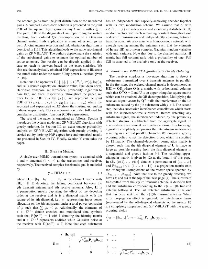
incomplete gamma function [20]. The result in (13) togetherwith Theorem 3 and (15) can be used to find the joint PDFof the squared layer gains of the first m substreams in anexact closed-form. The analytically obtained PDF expressionsfγ2(γ2) and fγ3(γ3) are plotted in Fig. 1 for t = 3 andr = 4 together with the corresponding simulated histograms.The strong match between the analytical and numerical resultsclearly verifies the accuracy of the analytical PDF expressions.

The CDF of γm can be written as given in (16) at thetop of the next page. The solutions to the integrals withinthe last expectation in (16) can be obtained from (15). Notethat the denominator term in (16) is not a function of γm.Also, as the average is taken over {γ1, γ2, . . . , γm−1}, wecan directly investigate the numerator to see the dependenceof the CDF on γm. As γm → 0, (15) can be replaced withO(γr−m+1

m ) by using asymptotic behavior of the incompletegamma functions [20]. Substituting this in (16), one canconclude

Fγm(γm) = O(γ(t−m+1)(r−m+1)m ) as γm → 0. (17)

Using the idea that an outage happens when the channel gainis sufficiently small (for high power allocation values), theexpression in (17) can be interpreted as that the mth substreamhas a diversity order of (t −m + 1)(r −m + 1) [4]. As theoverall outage probability of the ZF V-BLAST is dominatedby the worst subchannel gain, the overall diversity order is


Fγm(γm) = Eγ1,...,γm−1

{∫ γm

0

fγm1(γ1, γ2, . . . , γm−1, γm = z)

fγm−11

(γ1, γ2, . . . , γm−1)dz

}

= Eγ1,...,γm−1

⎧⎪⎨⎪⎩

(t−m+ 1)∫ γm

0

zr−m1

(r−m)!Im(γm = z1)[∫ z1

0

zr−m2

(r−m)!Im(γm = z2)dz2

]t−m

dz1[∫ γm−1

0

zr−m+13

(r−m+1)!Im−1(γm−1 = z3)dz3

]t−m+1

⎫⎪⎬⎪⎭

= Eγ1,...,γm−1

⎧⎪⎨⎪⎩

[∫ γm

0

zr−m1

(r−m)!Im(γm = z1)dz1

]t−m+1

[∫ γm−1

0

zr−m+13

(r−m+1)!Im−1(γm−1 = z3)dz3

]t−m+1

⎫⎪⎬⎪⎭ . (16)

0 1 2 3 4 5 6 70

0.1

0.2

0.3

0.4

0.5

0.6

0.7

γi

f γ i(γi)

Simulation, γ2

Analytical, γ2

Simulation, γ3

Analytical, γ3

Fig. 1. Comparison of the analytical PDF expressions on γ2 and γ3 withthe corresponding numerical results for t = 3 and r = 4.

given by (r − t+ 1) [6].

A. Low Rate Feedback of Decoding Order

When the transmitter is not provided with any form of CSI,the applicable capacity measure is the outage capacity [14].Representing the CDF of the ith layer’s squared gain byFγi(γi), the outage probability for the ith substream can bewritten as

Pout(Ri) = ε = Pr (log(1 + γiρi) ≤ Ri) = Fγi

(2Ri − 1

ρi

)(18)

for a given pair of rate and power allocation values Ri and ρi,respectively. Using (18), the ith substream’s ε−outage capacitycan be expressed as

Ri(ε) = log(1 + F−1

γi(ε)ρi

)(19)

where F−1γi

(.) denotes the inverse function for the CDF ofthe ith layer’s squared gain. It is worth to mention thatthe ith substream with the ε−outage capacity of Ri has(t− i+1)th place in detection order. Under an identical targetoutage probability of ε per layer, the optimal power alloca-tion policy that maximizes the sum of substream ε−outage

0 5 10 1510

−4

10−3

10−2

10−1

100

ρ (dB)

Pou

t (R

i = 1

bits

/s/H

z)

SimulationAnalytical

1st layer, i = 1

2nd layer, i = 2

3rd layer, i = 3

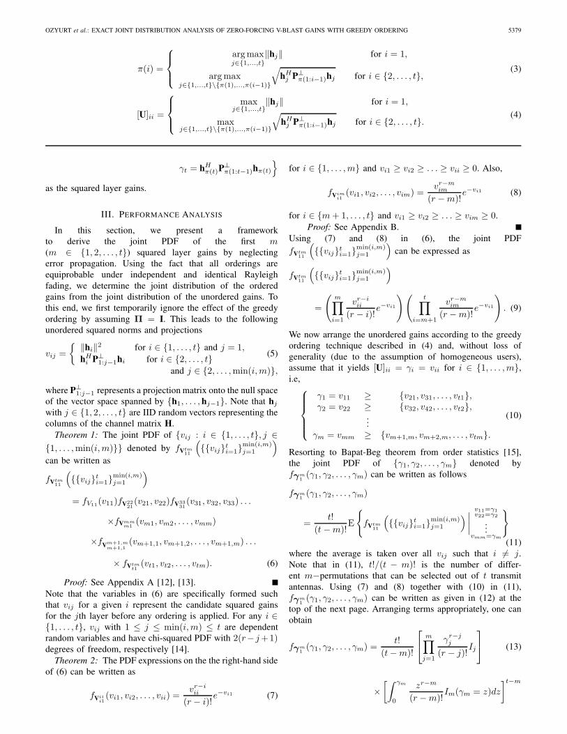
Fig. 2. Substream outage probabilities under a target rate of Ri = 1 bits/s/Hzwith t = 3, r = 4, and varying ρ.

capacities can be determined from

maxρi

t∑i=1

log(1 + F−1

γi(ε)ρi

),

subject tot∑

i=1

ρi = ρ. (20)

It can be shown that the optimal power allocation over layersis given by the following water-filling formula

ρi =

(μ− 1

F−1γi (ε)

)+

(21)

where (.)+ refers to max(0, .) and μ is obtained from∑ti=1 ρi = ρ [10]. For a given target ε outage probability

per layer and total power constraint of ρ, one can solve(21) beforehand (using the statistics of the squared layergains obtained previously) for the power allocation valuesand corresponding number of active substreams with nonzeropower allocations. In this case, the transmitter only needs tobe informed on the decoding order, which can be sent backfrom the receiver in log t! bits [10].

IV. NUMERICAL RESULTS

In this section, a number of numerical results are providedfor r = 4. The power allocation among substreams is uniform


0 5 10 150

2

4

6

8

10

12

ρ (dB)

Out

age

capa

city

(bi

ts/s

/Hz)

R

1+R

2+R

3, Greedy ordering

R1+R

2+R

3, No ordering

R1, Greedy ordering

R1, No ordering

R2, Greedy ordering

R2, No ordering

R3, Greedy ordering

R3, No ordering

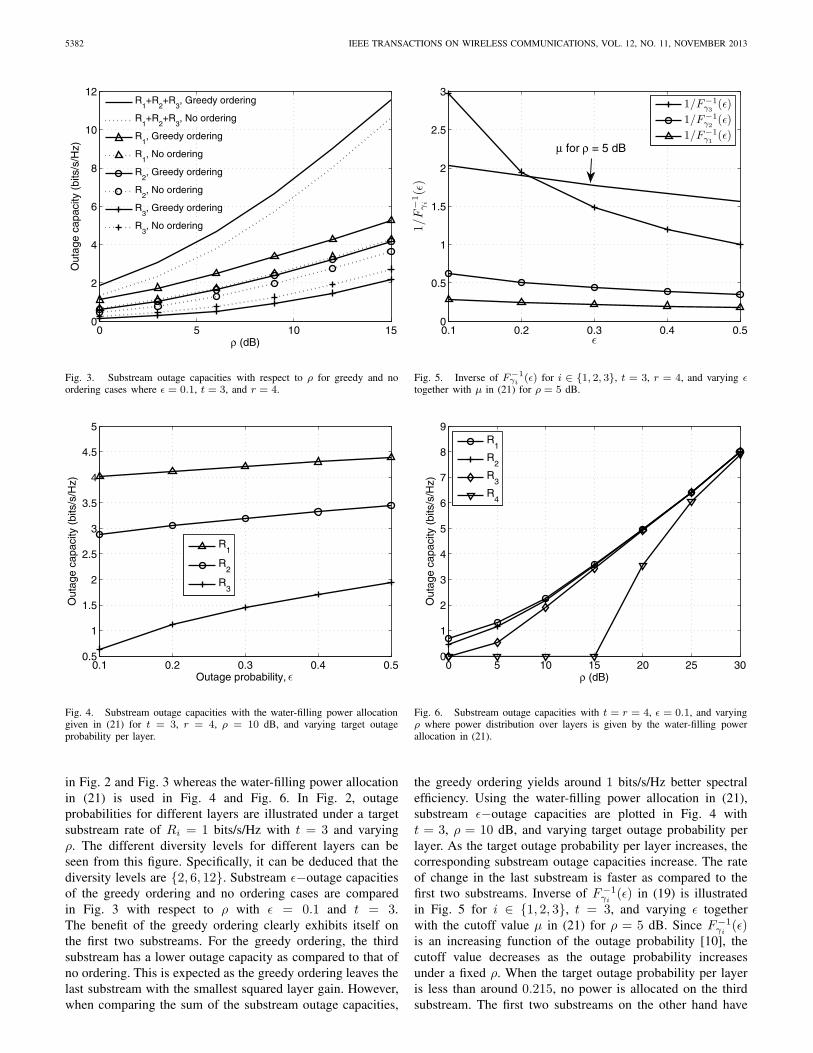
Fig. 3. Substream outage capacities with respect to ρ for greedy and noordering cases where ε = 0.1, t = 3, and r = 4.

0.1 0.2 0.3 0.4 0.50.5

1

1.5

2

2.5

3

3.5

4

4.5

5

Out

age

capa

city

(bi

ts/s

/Hz)

R1

R2

R3

εOutage probability,

Fig. 4. Substream outage capacities with the water-filling power allocationgiven in (21) for t = 3, r = 4, ρ = 10 dB, and varying target outageprobability per layer.

in Fig. 2 and Fig. 3 whereas the water-filling power allocationin (21) is used in Fig. 4 and Fig. 6. In Fig. 2, outageprobabilities for different layers are illustrated under a targetsubstream rate of Ri = 1 bits/s/Hz with t = 3 and varyingρ. The different diversity levels for different layers can beseen from this figure. Specifically, it can be deduced that thediversity levels are {2, 6, 12}. Substream ε−outage capacitiesof the greedy ordering and no ordering cases are comparedin Fig. 3 with respect to ρ with ε = 0.1 and t = 3.The benefit of the greedy ordering clearly exhibits itself onthe first two substreams. For the greedy ordering, the thirdsubstream has a lower outage capacity as compared to that ofno ordering. This is expected as the greedy ordering leaves thelast substream with the smallest squared layer gain. However,when comparing the sum of the substream outage capacities,

0.1 0.2 0.3 0.4 0.50

0.5

1

1.5

2

2.5

3

ε

1/F

−1

γi

(ε)

1/F−1

γ3(ε)

1/F−1γ2

(ε)1/F−1

γ1(ε)

μ for ρ = 5 dB

Fig. 5. Inverse of F−1γi (ε) for i ∈ {1, 2, 3}, t = 3, r = 4, and varying ε

together with μ in (21) for ρ = 5 dB.

0 5 10 15 20 25 300

1

2

3

4

5

6

7

8

9

ρ (dB)

Out

age

capa

city

(bi

ts/s

/Hz)

R1

R2

R3

R4

Fig. 6. Substream outage capacities with t = r = 4, ε = 0.1, and varyingρ where power distribution over layers is given by the water-filling powerallocation in (21).

the greedy ordering yields around 1 bits/s/Hz better spectralefficiency. Using the water-filling power allocation in (21),substream ε−outage capacities are plotted in Fig. 4 witht = 3, ρ = 10 dB, and varying target outage probability perlayer. As the target outage probability per layer increases, thecorresponding substream outage capacities increase. The rateof change in the last substream is faster as compared to thefirst two substreams. Inverse of F−1

γi(ε) in (19) is illustrated

in Fig. 5 for i ∈ {1, 2, 3}, t = 3, and varying ε togetherwith the cutoff value μ in (21) for ρ = 5 dB. Since F−1

γi(ε)

is an increasing function of the outage probability [10], thecutoff value decreases as the outage probability increasesunder a fixed ρ. When the target outage probability per layeris less than around 0.215, no power is allocated on the thirdsubstream. The first two substreams on the other hand have


similar nonzero power allocation values for all plotted range.Note that without the analytical CDF expressions, one mayneed to carry out extensive simulations to find the powerallocation values. For varying total available power ρ, thesubstream ε−outage capacities are plotted in Fig. 6 by settingt = 4 and ε = 0.1. Power allocation over layers is given bythe water-filling power allocation given in (21). When ρ issmall, the power allocation policy heavily favors the best twosubchannels resulting in a zero rate on the fourth substreamwhen ρ ≤ 15 dB. As ρ increases on the other hand, the powerdistribution over layers gets more and more uniform.

V. CONCLUSION

We have presented an exact statistical analysis on zero-forcing V-BLAST algorithm under no error propagation and agreedy selection of decoding order at the receiver. Relying onthe fact that all orderings are equiprobable under independentand identical Rayleigh fading, we have obtained the joint dis-tribution of the ordered gains using the joint distribution of theunordered gains. Unlike the previous approximate analyses, anexact mathematical framework has been introduced. Particu-larly, a compact and closed-form expression has been derivedon the joint PDF of the squared layer gains for any number oftransmit and receive antennas. The analytically obtained PDFexpressions have been utilized to compute the cutoff valueunder the water-filling power allocation that maximizes thesum of the substream outage capacities for a given sum powerconstraint [10]. It is also possible to extend our analysis toobtain exact bit and symbol error probability curves under noerror propagation. Our analysis has been numerically verified.The presented framework can be modified for other similarordering techniques.

APPENDIX APROOF OF THEOREM 1

The unordered variables {vij : i ∈ {1, . . . , t}, j ∈{1, . . . ,min(i,m)}} in (5) can be written as given in (22)at the top of the next page for m ≥ 3. In (22), hj forj ∈ {1, 2 . . . , t} represent the channel vectors (IID isotropicjointly Gaussian random vectors) and P⊥

1:j−1 is a projectionmatrix onto the null space of the vector space spanned by{h1, . . . , hj−1}. We need to prove that the random vec-tors [v11], [v21, v22], . . . , [vt1, vt2, . . . , vtm] are independent.Instead of working on the squared norms, we prove theindependence for the random vectors themselves given by (23)on the next page as a double-column equation. In other words,we prove that [w11], [w21,w22], . . . , [wt1,wt2, . . . ,wtm] areindependent. This is a stronger claim than the previous one,hence its proof directly implies the desired result. Note thatfor any wij = P⊥

1:j−1hi in (23), hi and P⊥1:j−1 are independent

since P⊥1:j−1 depends only on {h1, h2, . . . , hj−1} and we have

j ≤ i. Also, conditioned on {h1, h2, . . . , hj−1}, wij is a pro-jection of a Gaussian random vector onto a given subspace andhas a Gaussian distribution. This can be seen by first applyingthe spectral decomposition on P⊥

1:j−1 and then utilizing thefact that the distribution of a circularly-symmetric Gaussianrandom vector is invariant under unitary transformations [14].

Hence, the random vectors in a given row in (23) are jointlyGaussian. For Gaussian variates, pairwise independence im-plies joint independence as the dependence is establishedby the covariance matrix in this case. Consequently, provingpairwise independence for any two random vectors in differentrows serves our purpose. It is clear from the definition that allwi1 vectors with i ∈ {1, 2, . . . , t} are independent. As the pro-jections of two independent Gaussian random vectors onto agiven orthogonal direction (or subspace) are independent [14],all vectors in the second column, i.e, wi2 for i ∈ {2, 3, . . . , t},are also independent. The same result holds for all othercolumns. Hence, each column in (23) is comprised of IIDrandom vectors. Therefore, in order to prove Theorem 1, itsuffices to show that all pairs {wij ,wpq} with i �= p andj �= q are independent, i.e., E{wijwH

pq} = 0 with 0 denotingthe zero matrix. The product wijwH

pq can be written as

wijwHpq = P⊥

1:j−1hihHp P⊥

1:q−1 (24)

where we use the fact that any orthogonal projection matrixhas the property of being Hermitian. We can express (24) as

wijwHpq = P⊥

1:j−1hihHp P⊥

1:q−1 =r∑

ν=1

hiν gj−1,ν hHp P⊥

1:q−1

(25)where hiν and gj−1,ν with ν ∈ {1, 2, . . . , r} represent theνth element of hi and the νth column of P⊥

1:j−1, respectively.Taking average in (25), we can write

E{wijwHpq} =

r∑ν=1

E{hiν gj−1,ν hH

p P⊥1:q−1

}. (26)

We have j ≤ i, q ≤ p, i �= p, and j �= q. Also, gj−1,ν andP⊥1:q−1 depend only on {h1, . . . , hj−1} and {h1, . . . , hq−1},

respectively. Consequently, for p < i, (26) can be written as

E{wijwHpq} =

r∑ν=1

E {hiν} E{

gj−1,ν hHp P⊥

1:q−1

}= 0 (27)

since E {hiν} = 0. Using the same approach, (25) can alsobe expressed as

wijwHpq =

r∑ν=1

h∗pν P⊥

1:j−1hi gHq−1,ν (28)

where h∗pν and gq−1,ν with ν ∈ {1, 2, . . . , r} denote the

complex conjugate of the νth element of hp and the νthcolumn of P⊥

1:q−1, respectively. When p > i, hp is independentof hi, P⊥

1:j−1, and P⊥1:q−1. Additionally, as E

{h∗pν

}= 0, we

can conclude

E{

wijwHpq

}=

r∑ν=1

E{h∗pν

}E{

P⊥1:j−1hi gHq−1,ν

}= 0 (29)

for p > i.

APPENDIX BPROOF OF THEOREM 2

Let {βi1, . . . , βir} with i ∈ {1, . . . , t} be independentand exponentially distributed random variables. Also, forj ∈ {1, . . . , r}, define vij as

vij = βij + . . .+ βir . (30)


v11 = ‖h1‖2,v21 = ‖h2‖2, v22 = ‖P⊥

1 h2‖2,v31 = ‖h3‖2, v32 = ‖P⊥

1 h3‖2, v33 = ‖P⊥1:2h3‖2,

......

...vm1 = ‖hm‖2, vm2 = ‖P⊥

1 hm‖2, vm3 = ‖P⊥1:2hm‖2, . . . , vmm = ‖P⊥

1:m−1hm‖2,...

......

......

vt1 = ‖ht‖2, vt2 = ‖P⊥1 ht‖2, vt3 = ‖P⊥

1:2ht‖2, . . . , vtm = ‖P⊥1:m−1ht‖2.

(22)

w11 = h1,

w21 = h2, w22 = P⊥1 h2,

w31 = h3, w32 = P⊥1 h3, w33 = P⊥

1:2h3,...

......

wm1 = hm, wm2 = P⊥1 hm, wm3 = P⊥

1:2hm, . . . , wmm = P⊥1:m−1hm,

......

......

...wt1 = ht, wt2 = P⊥

1 ht, wt3 = P⊥1:2ht, . . . , wtm = P⊥

1:m−1ht.

(23)

In (30), {βi1, . . . , βir} have the following joint PDF

fβir

i1

(βi1, . . . , βir) = e−(βi1+...+βir) (31)

for {βi1, . . . , βir} ≥ 0 [14]. Using (30), we can derive thefollowing transformation:

βij =

{vij − vi,j+1 for j ∈ {1, . . . , r − 1},vir for j = r,

(32)

with the Jacobian determinant given by det(J) = 1. Using(31) and (32), we can write

f˜Vir

i1(vi1, . . . , vir) = fβir

i1

(βi1 = vi1 − vi2, βi2 = vi2 − vi3,

. . . , βir = vir) | det(J)|= e−vi1 (33)

for vi1 ≥ . . . ≥ vir ≥ 0. Note that we have vij = vij fori ∈ {1, . . . , t} and j ∈ {1, . . . , i}. Therefore, the joint PDF of{vi1, vi2, . . . , vii} is identical to that of {vi1, vi2, . . . , vii} andcan be determined by integrating out {vi,i+1, vi,i+2, . . . , vir}in (33). This fact can be utilized to obtain (7) and (8).

APPENDIX CPROOF OF THEOREM 3

The multiple integral Ij is defined as

Ij =

∫ γj−1

γj

∫ γj−2

vj,j−1

. . .

∫ γ1

vj2

e−vj1dvj1 . . . dvj,j−2 dvj,j−1

for γ1 ≥ γ2 ≥ . . . ≥ γm ≥ 0. This integral also appearsin [17] where the authors use some bounding techniques toget an approximated solution. We first evaluate the innermostintegral as

Ij =

∫ γj−1

γj

∫ γj−2

vj,j−1

. . .

∫ γ2

vj3

(e−vj2 − e−γ1

)dvj2

. . . dvj,j−2 dvj,j−1.

Partially solving the new innermost integral, we obtain

Ij =

∫ γj−1

γj

∫ γj−2

vj,j−1

. . .

∫ γ3

vj4

(e−vj3 − e−γ2

)dvj3 . . .

dvj,j−2 dvj,j−1

−e−γ1

∫ γj−1

γj

∫ γj−2

vj,j−1

. . .

∫ γ2

vj3

dvj2 . . . dvj,j−2 dvj,j−1.

Proceeding in the same way, we can conclude

Ij = e−γj − e−γj−1 − e−γj−2 (γj−1 − γj)−j−3∑k=1

e−γj−k−2

×[G(γj−1, γj−2, γj−3, . . . , γj−k−1) (34)

−G(γj , γj−2, γj−3, . . . , γj−k−1)

]

where

G(α1, α2, . . . , αk+1)

=

∫ α1

0

∫ α2

xk+1

∫ α3

xk

. . .

∫ αk+1

x2

dx1 dx2 . . . dxk dxk+1

with 0 ≤ α1 ≤ α2 ≤ . . . ≤ αk+1.

Lemma 1: The solution to the multiple integralG(α1, α2, . . . , αk+1) is given in [21] as

G(α1, α2, . . . , αk+1)

=∑

b1+...+bk+1=k+1∀n∈{1,...,k},b1+...+bn≤n

αbk+1

1 (α2 − α1)bk . . . (αk+1 − αk)

b1

bk+1!bk! . . . b1!

(35)where the summation is evaluated over allcombinations of nonnegative integer indices {bk+1,


bk, . . . , b1} (starting from bk+1) with the condition thatthe listed requirements are satisfied.

Using (35) in (34), the desired result in (14) can be obtained.

REFERENCES

[1] G. J. Foschini and M. J. Gans, “On limits of wireless communications ina fading environment when using multiple antennas,” Wireless PersonalCommun., vol. 6, no. 3, pp. 311–335, Mar. 1998.

[2] I. E. Telatar, “Capacity of multi-antenna Gaussian channels,” EuropeanTrans. Telecommun., vol. 10, no. 6, pp. 585–595, Dec. 1999.

[3] G. J. Foschini, G. D. Golden, R. A. Valenzuela, and P. W. Wolniansky,“Detection algorithm and initial laboratory results using V-BLASTspace-time communication architecture,” Electron. Lett., vol. 35, no. 1,pp. 14–16, Jan. 1999.

[4] Y. Jiang and M. K. Varanasi, “Spatial multiplexing architectures withjointly designed rate-tailoring and ordered BLAST decoding—part I:diversity-multiplexing tradeoff analysis,” IEEE Trans. Wireless Com-mun., vol. 7, no. 8, pp. 3252–3261, Aug. 2008.

[5] R. Narasimhan, “Error propagation analysis of V-BLAST with channel-estimation errors,” IEEE Trans. Commun., vol. 53, no. 1, pp. 27–31,Jan. 2005.

[6] S. Loyka and F. Gagnon, “Performance analysis of the V-BLASTalgorithm: an analytical approach,” IEEE Trans. Wireless Commun., vol.3, no. 4, pp. 1326–1337, July 2004.

[7] Y. Jiang, M. K. Varanasi, and J. Li, “Performance analysis of ZF andMMSE equalizers for MIMO systems: an in-depth study of the highSNR regime,” IEEE Trans. Inf. Theory, vol. 57, no. 4, pp. 2008–2026,Apr. 2011.

[8] H. Zhang, H. Dai, and B. L. Hughes, “Analysis on the diversity-multiplexing tradeoff for ordered MIMO SIC receivers,” IEEE Trans.Commun., vol. 57, no. 1, pp. 125–133, Jan. 2009.

[9] S. Loyka and F. Gagnon, “On outage and error rate analysis of theordered V-BLAST,” IEEE Trans. Wireless Commun., vol. 7, no. 10, pp.3679–3685, Oct. 2008.

[10] Y. Jiang and M. K. Varanasi, “Spatial multiplexing architectures withjointly designed rate-tailoring and ordered BLAST decoding—part II: apractical method for rate and power allocation,” IEEE Trans. WirelessCommun., vol. 7, no. 8, pp. 3262–3271, Aug. 2008.

[11] Q. Zhou and H. Dai, “Joint antenna selection and link adaptation forMIMO systems,” IEEE Trans. Veh. Technol., vol. 55, no. 1, pp. 243–255,Jan. 2006.

[12] S. Ozyurt and M. Torlak, “Unified performance analysis of orthogo-nal transmit beamforming methods with user selection,” IEEE Trans.Wireless Commun., vol. 12, no. 3, pp. 1026–1037, Mar. 2013.

[13] S. Ozyurt and M. Torlak, “Performance analysis of optimum zero-forcing beamforming with greedy user selection,” IEEE Commun. Lett.,vol. 16, no. 4, pp. 446–449, Apr. 2012.

[14] D. Tse and P. Viswanath, Fundamentals of Wireless Communication.Cambridge University Press, 2005.

[15] H. A. David and H. N. Nagaraja, Order Statistics, 3rd ed. Wiley, 2003.[16] S. Ozyurt and M. Torlak, “An exact outage analysis of zero-forcing V-

BLAST with greedy ordering,” in Proc. 2011 IEEE Global Commun.Conf.-Broad. Wireless Access Work.

[17] G. Dimic and N. D. Sidiropoulos, “On downlink beamforming withgreedy user selection: performance analysis and a simple new algo-rithm,” IEEE Trans. Signal Process., vol. 53, no. 10, pp. 3857–3868,Oct. 2005.

[18] G. Caire and S. Shamai, “On the achievable throughput of a multi-antenna Gaussian broadcast channel,” IEEE Trans. Inf. Theory, vol. 49,no. 7, pp. 1691–1706, July 2003.

[19] Z. Tu and R. S. Blum, “Multiuser diversity for a dirty paper approach,”IEEE Commun. Lett., vol. 7, no. 8, pp. 370–372, Aug. 2003.

[20] I. Gradshteyn and I. Ryzhik, Table of Integrals, Series, and Products.Academic Press, 2000.

[21] S. S. Wilks, “Order statistics,” Bull. Amer. Math. Soc., vol. 54, no. 1,pp. 6–50, Jan. 1948.

Serdar Ozyurt received the B.Sc. degree in electri-cal and electronics engineering from Sakarya Uni-versity, Turkey, in 2001, the M.Sc. degree in elec-tronics engineering from Gebze Institute of Tech-nology, Turkey, in 2005, and the Ph.D. degree inelectrical engineering from University of Texas atDallas, USA, in 2012. He is now an AssistantProfessor in the Department of Energy SystemsEngineering, Yildirim Beyazit University, Ankara,Turkey. His current research interests include multi-antenna communication systems with multiple users

and related signal processing techniques.

Murat Torlak received M.S. and Ph.D. degrees inelectrical engineering from The University of Texasat Austin in 1995 and 1999, respectively. He is anAssociate Professor in the Department of ElectricalEngineering at the Eric Johnson School of Engi-neering and Computer Science within the Universityof Texas at Dallas. He spent the summers of 1997and 1998 in Cwill Telecommunications, Inc., Austin,TX, where he participated in the design of a smartantenna wireless local loop system and directedresearch and development efforts towards standard-

ization of TD-SCDMA for the International Telecommunication Union. Hewas a visiting scholar at University of California Berkeley during 2008. Hehas been an active contributor in the areas of smart antennas and multiuserdetection. His current research focus is on experimental platforms for multipleantenna systems, millimeter wave systems, and wireless communications withhealth care applications. He is an Associate Editor of IEEE TRANSACTIONS

ON WIRELESS COMMUNICATIONS. He was the Program Chair of IEEESignal Processing Society Dallas Chapter during 2003-2005. He is a SeniorIEEE member. He has served on the Technical Program Committees (TPC)of the several IEEE conferences.

Documents

Exact Joint Distribution Analysis of Zero-Forcing V-BLAST Gains with Greedy Ordering