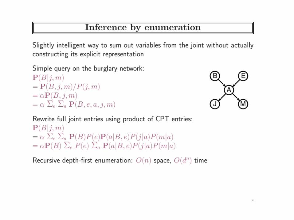
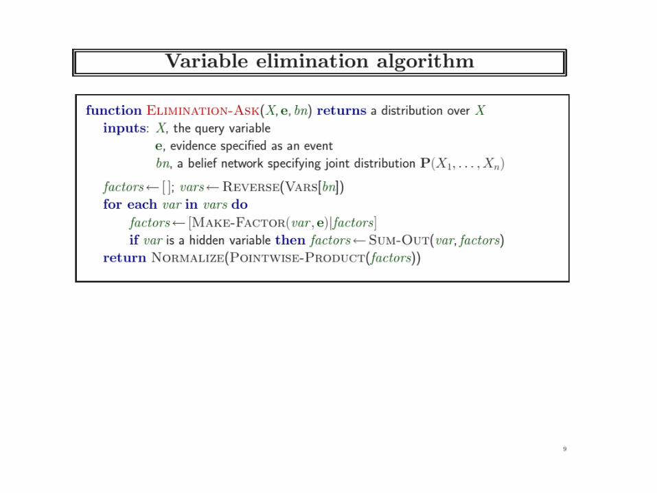
Exact Inference

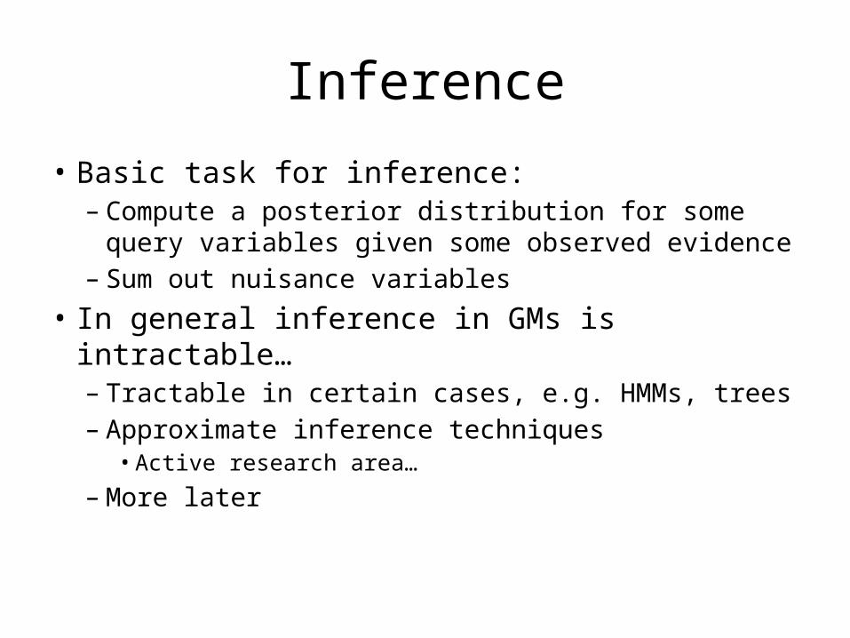
Inference

• Basic task for inference:– Compute a posterior distribution for some query

variables given some observed evidence– Sum out nuisance variables

• In general inference in GMs is intractable…– Tractable in certain cases, e.g. HMMs, trees– Approximate inference techniques• Active research area…

– More later

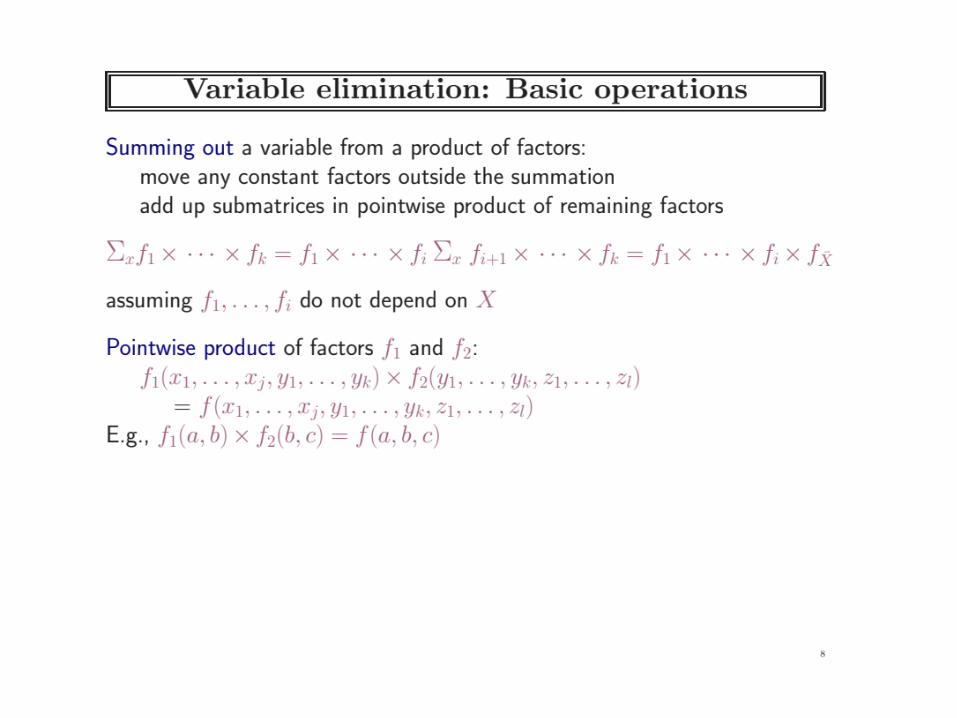
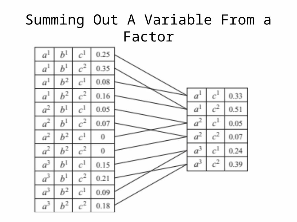
Summing Out A Variable From a Factor

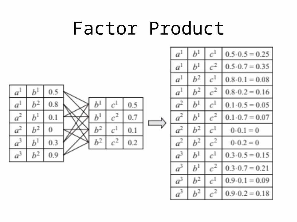
Factor Product

Belief Propagation: Motivation

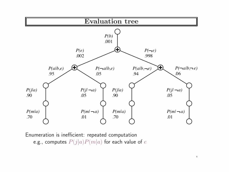
• What if we want to compute all marginals, not just one?

• Doing variable elimination for each onein turn is inefficient

• Solution: Belief Propagation– Same idea as Forward-backward for HMMs

Belief Propagation

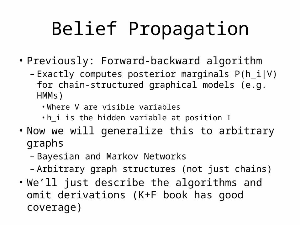
• Previously: Forward-backward algorithm– Exactly computes posterior marginals P(h_i|V) for

chain-structured graphical models (e.g. HMMs)• Where V are visible variables• h_i is the hidden variable at position I

• Now we will generalize this to arbitrary graphs– Bayesian and Markov Networks– Arbitrary graph structures (not just chains)

• We’ll just describe the algorithms and omit derivations (K+F book has good coverage)

BP: Initial Assumptions

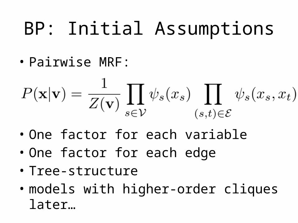
• Pairwise MRF:

• One factor for each variable• One factor for each edge• Tree-structure• models with higher-order cliques later…

Belief Propagation

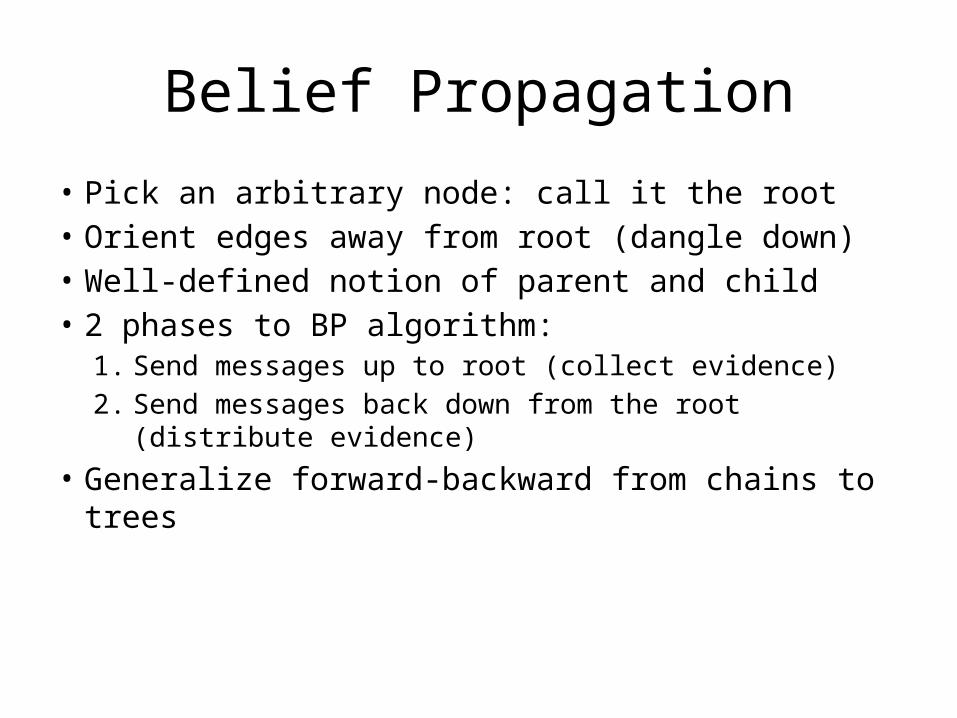
• Pick an arbitrary node: call it the root• Orient edges away from root (dangle down)• Well-defined notion of parent and child• 2 phases to BP algorithm:

1. Send messages up to root (collect evidence)2. Send messages back down from the root

(distribute evidence)• Generalize forward-backward from chains to

trees

Collect to root phase

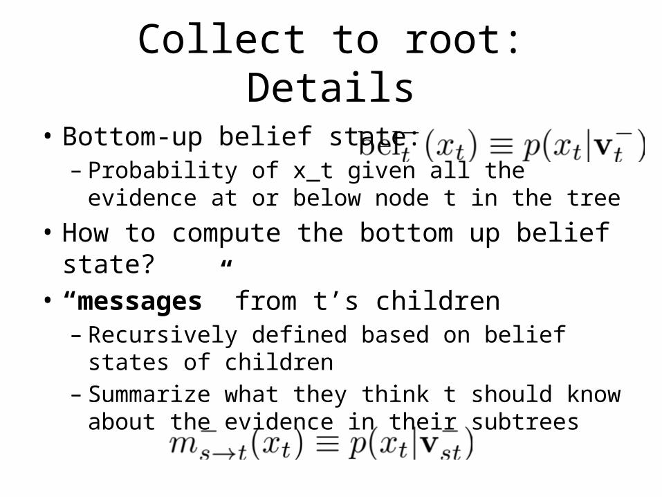
Collect to root: Details

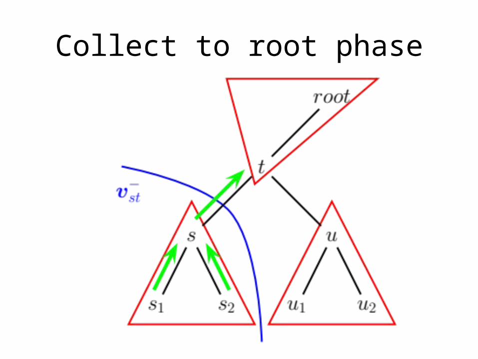
• Bottom-up belief state:– Probability of x_t given all the evidence at or

below node t in the tree• How to compute the bottom up belief state?• “messages” from t’s children – Recursively defined based on belief states of

children– Summarize what they think t should know about

the evidence in their subtrees

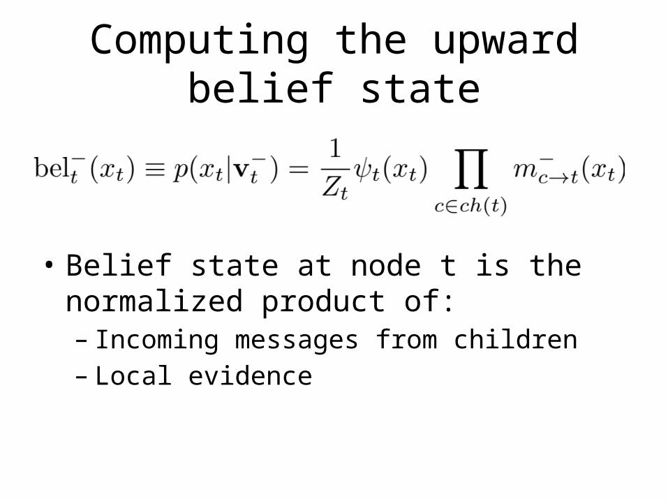
Computing the upward belief state

• Belief state at node t is the normalized product of:– Incoming messages from children– Local evidence

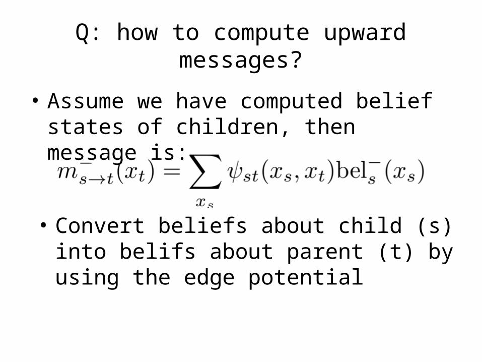
Q: how to compute upward messages?

• Assume we have computed belief states of children, then message is:

• Convert beliefs about child (s) into belifs about parent (t) by using the edge potential

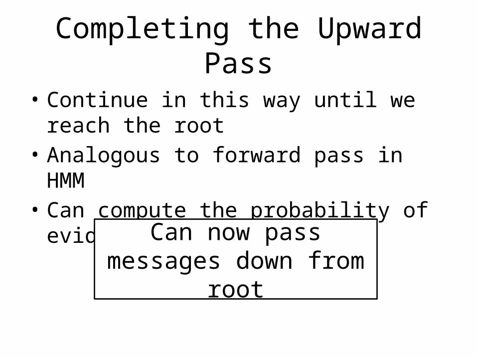
Completing the Upward Pass

• Continue in this way until we reach the root• Analogous to forward pass in HMM• Can compute the probability of evidence as a

side effect

Can now pass messages down from root

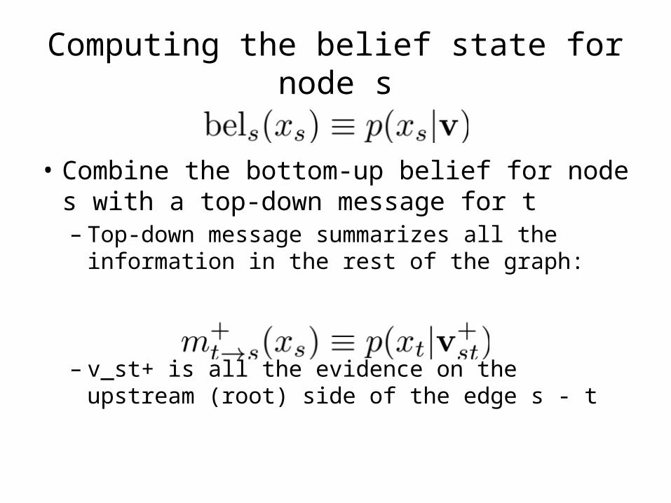
Computing the belief state for node s

• Combine the bottom-up belief for node s with a top-down message for t– Top-down message summarizes all the

information in the rest of the graph:

– v_st+ is all the evidence on the upstream (root) side of the edge s - t

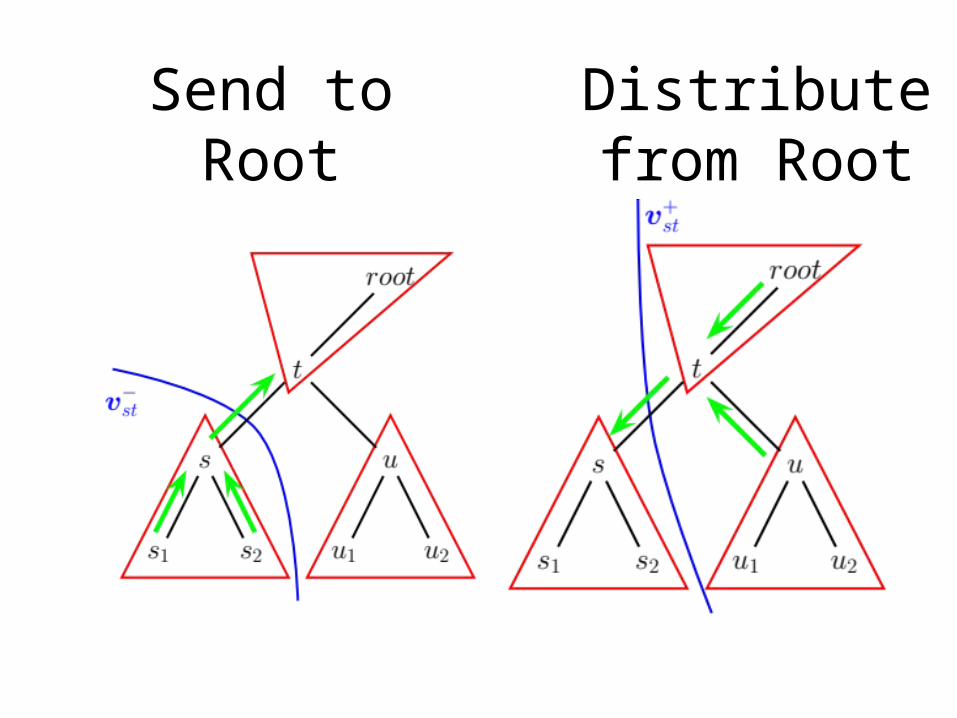
Distribute from RootSend to Root

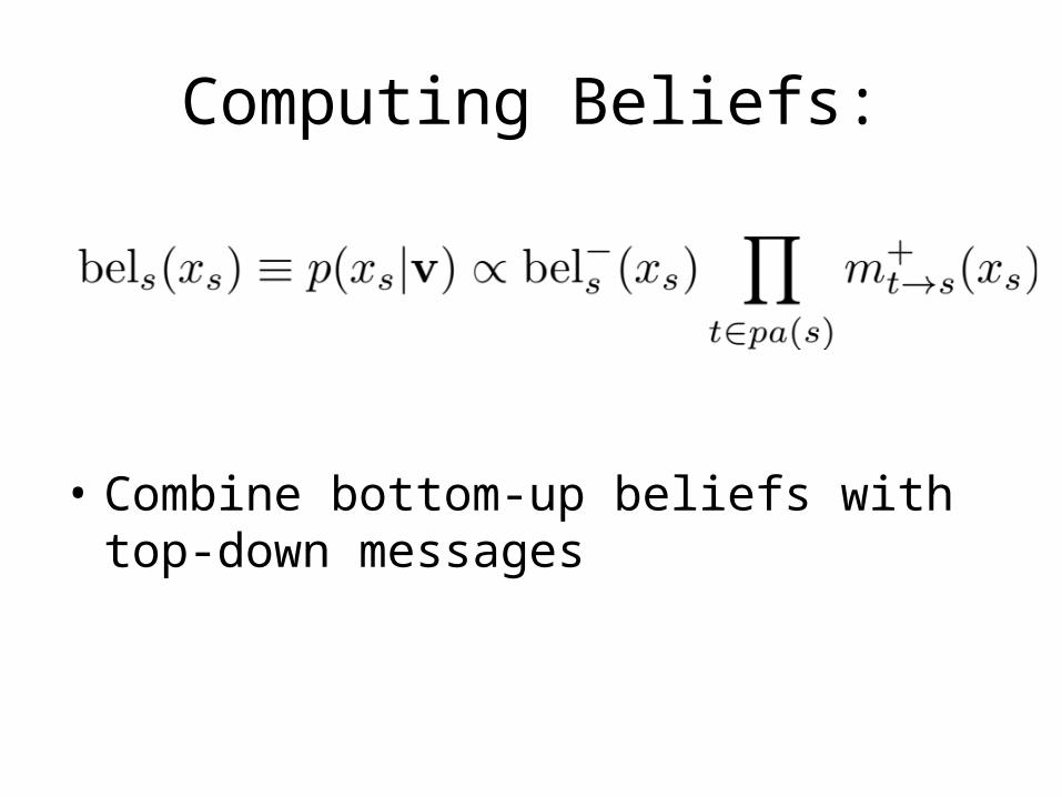
Computing Beliefs:

• Combine bottom-up beliefs with top-down messages

Q: how to compute top-down messages?

• Consider the message from t to s• Suppose t’s parent is r• t’s children are s and u• (like in the figure)

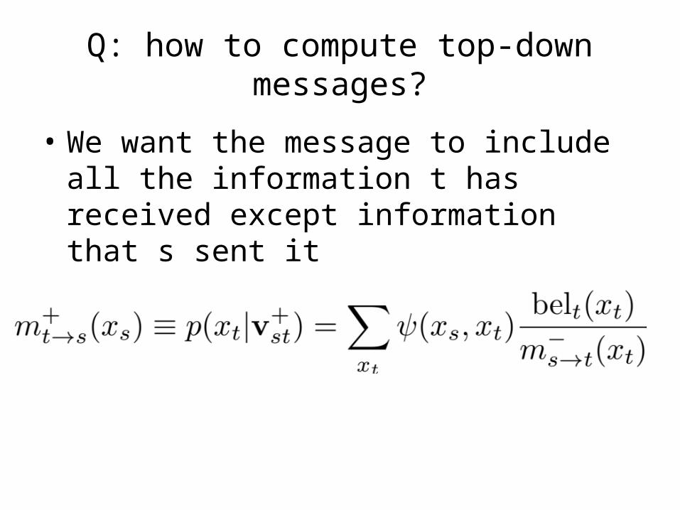
Q: how to compute top-down messages?

• We want the message to include all the information t has received except information that s sent it

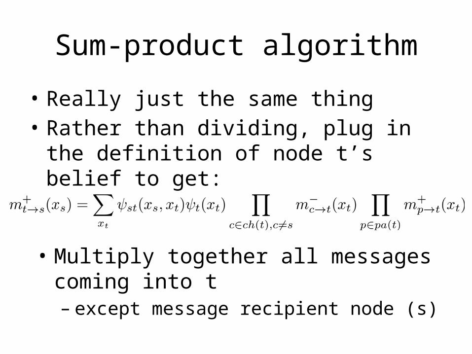
Sum-product algorithm

• Really just the same thing• Rather than dividing, plug in the definition of

node t’s belief to get:

• Multiply together all messages coming into t– except message recipient node (s)

Parallel BP

• So far we described the “serial” version– This is optimal for tree-structured GMs– Natural extension of forward-backward

• Can also do in parallel– All nodes receive messages from their neighbors in

parallel– Initialize messages to all 1’s– Each node absorbs messages from all it’s neighbors– Each node sends messages to each of it’s neighbors

• Converges to the correct posterior marginal

Loopy BP

• Approach to “approximate inference”• BP is only guaranteed to give the correct

answer on tree-structured graphs• But, can run it on graphs with loops, and it

gives an approximate answer– Sometimes doesn’t converge

Generalized Distributive Law

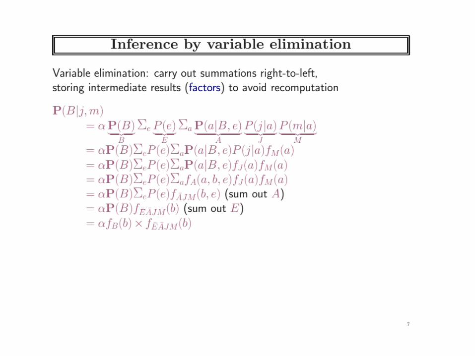
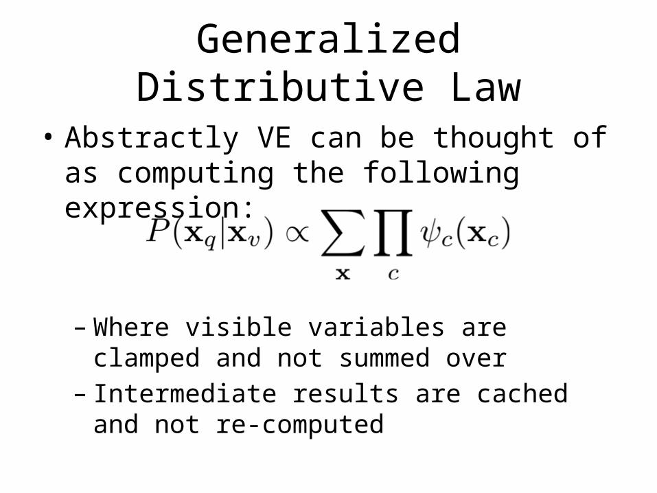
• Abstractly VE can be thought of as computing the following expression:

– Where visible variables are clamped and not summed over

– Intermediate results are cached and not re-computed

Generalized Distributive Law

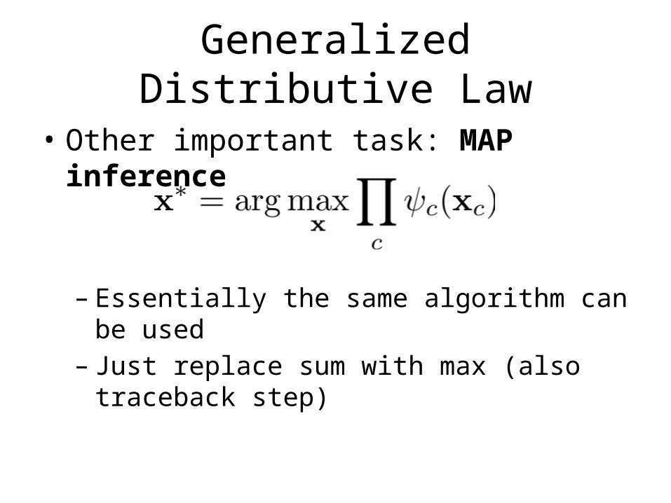
• Other important task: MAP inference

– Essentially the same algorithm can be used– Just replace sum with max (also traceback step)

Generalized Distributive Law

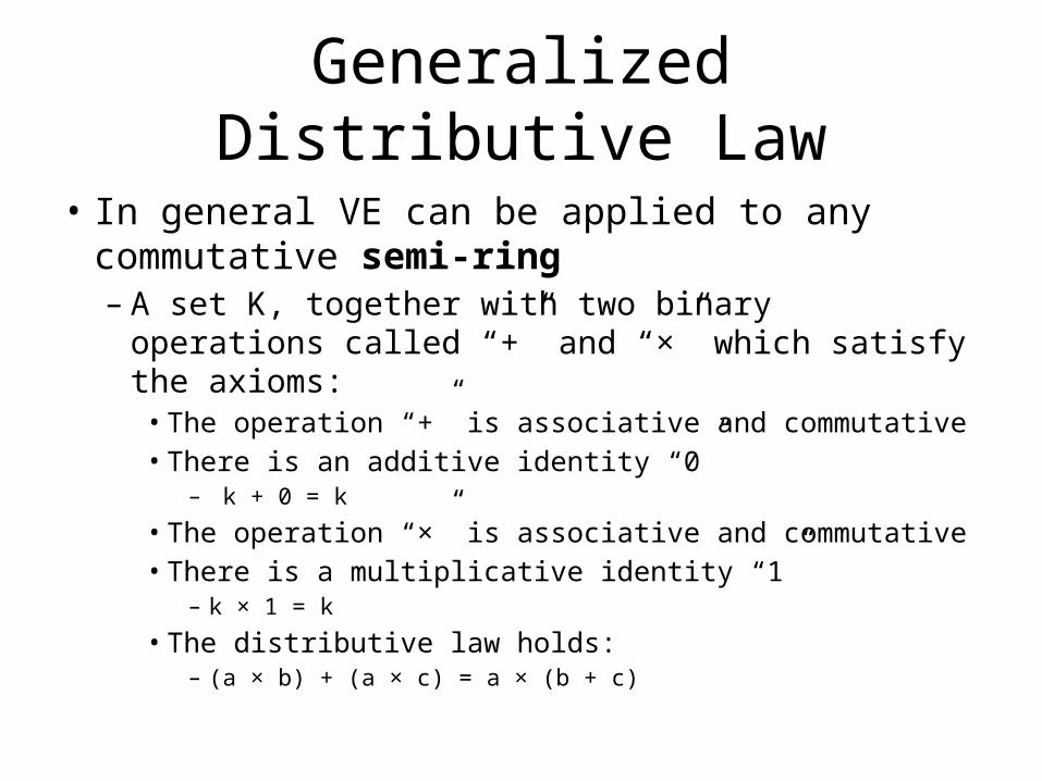
• In general VE can be applied to any commutative semi-ring– A set K, together with two binary operations called “+”

and “×” which satisfy the axioms:• The operation “+” is associative and commutative• There is an additive identity “0”

– k + 0 = k

• The operation “×” is associative and commutative• There is a multiplicative identity “1”

– k × 1 = k

• The distributive law holds:– (a × b) + (a × c) = a × (b + c)

Generalized Distributive Law

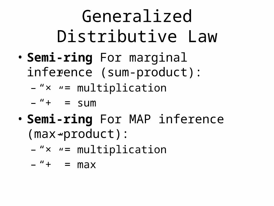
• Semi-ring For marginal inference (sum-product):– “×” = multiplication– “+” = sum

• Semi-ring For MAP inference (max-product):– “×” = multiplication– “+” = max