Evolutionary Search

Artificial Intelligence

CSPP 56553

January 28, 2004

Agenda

• Motivation:– Evolving a solution

• Genetic Algorithms– Modeling search as evolution

• Mutation

• Crossover

• Survival of the fittest

• Survival of the most diverse

• Conclusions

Genetic Algorithms Applications

• Search parameter space for optimal assignment– Not guaranteed to find optimal, but can approach

• Classic optimization problems:– E.g. Traveling Salesman Problem

• Program design (“Genetic Programming”)

• Aircraft carrier landings

Genetic Algorithms Procedure

• Create an initial population (1 chromosome)• Mutate 1+ genes in 1+ chromosomes

– Produce one offspring for each chromosome

• Mate 1+ pairs of chromosomes with crossover• Add mutated & offspring chromosomes to pop• Create new population

– Best + randomly selected (biased by fitness)

Fitness

• Natural selection: Most fit survive

• Fitness= Probability of survival to next gen

• Question: How do we measure fitness?– “Standard method”: Relate fitness to quality

• :0-1; :1-9:

Chromosome Quality Fitness

1 43 11 21 1

4321

0.40.30.20.1

if iq j jii qqf

Crossover

• Genetic design: – Identify sets of features: 2 genes:

flour+sugar;1-9

• Population: How many chromosomes?– 1 initial, 4 max

• Mutation: How frequent?– 1 gene randomly selected, randomly mutated

• Crossover: Allowed? Yes, select random mates; cross at middle

• Duplicates? No• Survival: Standard method

Basic Cookie GA+Crossover Results

• Results are for 1000 random trials– Initial state: 1 1-1, quality 1 chromosome

• On average, reaches max quality (9) in 14 generations

• Conclusion:– Faster with crossover: combine good in each gene– Key: Global max achievable by maximizing each

dimension independently - reduce dimensionality

Solving the Moat Problem

• Problem:– No single step mutation

can reach optimal values using standard fitness (quality=0 => probability=0)

• Solution A:– Crossover can combine fit

parents in EACH gene

• However, still slow: 155 generations on average

1 2 3 4 5 4 3 2 123454321

0 0 0 0 0 0 0 20 0 0 0 0 0 0 30 0 7 8 7 0 0 40 0 8 9 8 0 0 50 0 7 8 7 0 0 40 0 0 0 0 0 0 30 0 0 0 0 0 0 22 3 4 5 4 3 2 1

Questions

• How can we avoid the 0 quality problem?

• How can we avoid local maxima?

Rethinking Fitness

• Goal: Explicit bias to best– Remove implicit biases based on quality

scale

• Solution: Rank method– Ignore actual quality values except for ranking

• Step 1: Rank candidates by quality• Step 2: Probability of selecting ith candidate, given

that i-1 candidate not selected, is constant p. – Step 2b: Last candidate is selected if no other has been

• Step 3: Select candidates using the probabilities

Rank Method

Chromosome Quality Rank Std. Fitness Rank Fitness

1 41 31 25 27 5

4 3 2 1 0

1 2345

0.4 0.30.20.10.0

0.667 0.2220.0740.0250.012

Results: Average over 1000 random runs on Moat problem- 75 Generations (vs 155 for standard method)

No 0 probability entries: Based on rank not absolute quality

Diversity

• Diversity: – Degree to which chromosomes exhibit

different genes– Rank & Standard methods look only at quality– Need diversity: escape local min, variety for

crossover– “As good to be different as to be fit”

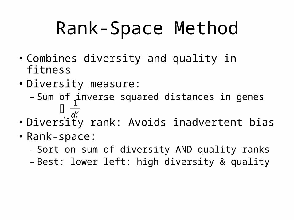
Rank-Space Method

• Combines diversity and quality in fitness• Diversity measure:

– Sum of inverse squared distances in genes

• Diversity rank: Avoids inadvertent bias• Rank-space:

– Sort on sum of diversity AND quality ranks– Best: lower left: high diversity & quality

i id

2

1

Rank-Space Method

Chromosome Q D D Rank Q Rank Comb Rank R-S Fitness

1 43 11 21 17 5

4 3 2 1 0

1 5342

1 2345

0.667 0.0250.2220.0120.074

Diversity rank breaks tiesAfter select others, sum distances to bothResults: Average (Moat) 15 generations

0.04 0.25 0.059 0.062 0.05

1 4253

W.r.t. highest ranked 5-1

Genetic Algorithms

• Evolution mechanisms as search technique– Produce offspring with variation

• Mutation, Crossover

– Select “fittest” to continue to next generation• Fitness: Probability of survival

– Standard: Quality values only– Rank: Quality rank only– Rank-space: Rank of sum of quality & diversity ranks

• Large population can be robust to local max

Machine Learning:Nearest Neighbor &

Information Retrieval SearchArtificial Intelligence

CSPP 56553

January 28, 2004

Agenda

• Machine learning: Introduction• Nearest neighbor techniques

– Applications: Robotic motion, Credit rating– Information retrieval search

• Efficient implementations:– k-d trees, parallelism

• Extensions: K-nearest neighbor• Limitations:

– Distance, dimensions, & irrelevant attributes

Machine Learning

• Learning: Acquiring a function, based on past inputs and values, from new inputs to values.

• Learn concepts, classifications, values– Identify regularities in data

Machine Learning Examples

• Pronunciation: – Spelling of word => sounds

• Speech recognition:– Acoustic signals => sentences

• Robot arm manipulation:– Target => torques

• Credit rating:– Financial data => loan qualification

Machine Learning Characterization

• Distinctions:– Are output values known for any inputs?

• Supervised vs unsupervised learning– Supervised: training consists of inputs + true output

value» E.g. letters+pronunciation

– Unsupervised: training consists only of inputs» E.g. letters only

• Course studies supervised methods

Machine Learning Characterization

• Distinctions:– Are output values discrete or continuous?

• Discrete: “Classification”– E.g. Qualified/Unqualified for a loan application

• Continuous: “Regression”– E.g. Torques for robot arm motion

• Characteristic of task

Machine Learning Characterization

• Distinctions:– What form of function is learned?

• Also called “inductive bias”• Graphically, decision boundary• E.g. Single, linear separator

– Rectangular boundaries - ID trees– Vornoi spaces…etc…

+ + + - - -

Machine Learning Functions

• Problem: Can the representation effectively model the class to be learned?

• Motivates selection of learning algorithm

++ + + + +

- - - - - - - - -

For this function,Linear discriminant is GREAT!Rectangular boundaries (e.g. ID trees)

TERRIBLE!

Pick the right representation!

Machine Learning Features

• Inputs: – E.g.words, acoustic measurements, financial

data– Vectors of features:

• E.g. word: letters – ‘cat’: L1=c; L2 = a; L3 = t

• Financial data: F1= # late payments/yr : Integer• F2 = Ratio of income to expense:

Real

Machine Learning Features

• Question: – Which features should be used?– How should they relate to each other?

• Issue 1: How do we define relation in feature space if features have different scales? – Solution: Scaling/normalization

• Issue 2: Which ones are important?– If differ in irrelevant feature, should ignore

Complexity & Generalization

• Goal: Predict values accurately on new inputs• Problem:

– Train on sample data– Can make arbitrarily complex model to fit– BUT, will probably perform badly on NEW data

• Strategy:– Limit complexity of model (e.g. degree of equ’n)– Split training and validation sets

• Hold out data to check for overfitting

Nearest Neighbor

• Memory- or case- based learning

• Supervised method: Training– Record labeled instances and feature-value vectors

• For each new, unlabeled instance– Identify “nearest” labeled instance– Assign same label

• Consistency heuristic: Assume that a property is the same as that of the nearest reference case.

Nearest Neighbor Example

• Problem: Robot arm motion– Difficult to model analytically

• Kinematic equations – Relate joint angles and manipulator positions

• Dynamics equations– Relate motor torques to joint angles

– Difficult to achieve good results modeling robotic arms or human arm

• Many factors & measurements

Nearest Neighbor Example

• Solution: – Move robot arm around– Record parameters and trajectory segment

• Table: torques, positions,velocities, squared velocities, velocity products, accelerations

– To follow a new path:• Break into segments • Find closest segments in table• Get those torques (interpolate as necessary)

Nearest Neighbor Example

• Issue: Big table– First time with new trajectory

• “Closest” isn’t close• Table is sparse - few entries

• Solution: Practice– As attempt trajectory, fill in more of table

• After few attempts, very close

Roadmap

• Problem: – Matching Topics and Documents

• Methods:– Classic: Vector Space Model

• Challenge I: Beyond literal matching– Expansion Strategies

• Challenge II: Authoritative source– Page Rank– Hubs & Authorities

Matching Topics and Documents

• Two main perspectives:– Pre-defined, fixed, finite topics:

• “Text Classification”

– Arbitrary topics, typically defined by statement of information need (aka query)

• “Information Retrieval”

Three Steps to IR● Three phases:

– Indexing: Build collection of document representations

– Query construction:● Convert query text to vector

– Retrieval:● Compute similarity between query and doc

representation● Return closest match

Matching Topics and Documents

• Documents are “about” some topic(s)• Question: Evidence of “aboutness”?

– Words !!• Possibly also meta-data in documents

– Tags, etc

• Model encodes how words capture topic– E.g. “Bag of words” model, Boolean matching– What information is captured?– How is similarity computed?

Models for Retrieval and Classification

• Plethora of models are used

• Here:– Vector Space Model

Vector Space Information Retrieval

• Task:– Document collection– Query specifies information need: free text– Relevance judgments: 0/1 for all docs

• Word evidence: Bag of words– No ordering information

Vector Space Model

Computer

Tv

Program

Two documents: computer program, tv programQuery: computer program : matches 1 st doc: exact: distance=2 vs 0 educational program: matches both equally: distance=1

Vector Space Model

• Represent documents and queries as– Vectors of term-based features

• Features: tied to occurrence of terms in collection

– E.g.

• Solution 1: Binary features: t=1 if present, 0 otherwise– Similiarity: number of terms in common

• Dot product

),...,,();,...,,( ,,2,1,,2,1 kNkkkjNjjj tttqtttd

ji

N

ikijk ttdqsim ,

1,),(

Question

• What’s wrong with this?

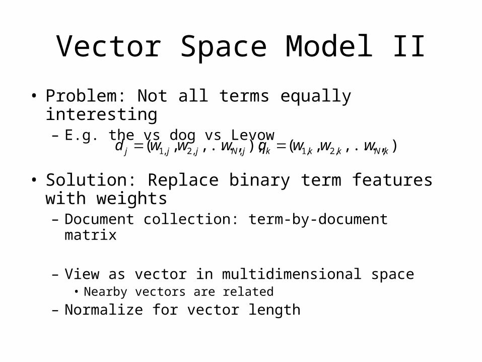
Vector Space Model II

• Problem: Not all terms equally interesting– E.g. the vs dog vs Levow

• Solution: Replace binary term features with weights– Document collection: term-by-document matrix

– View as vector in multidimensional space• Nearby vectors are related

– Normalize for vector length

),...,,();,...,,( ,,2,1,,2,1 kNkkkjNjjj wwwqwwwd

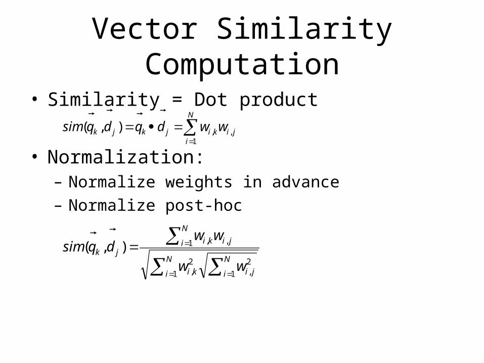
Vector Similarity Computation

• Similarity = Dot product

• Normalization:– Normalize weights in advance– Normalize post-hoc

ji

N

ikijkjk wwdqdqsim ,

1,),(

N

i ji

N

i ki

N

i jikijk

ww

wwdqsim

1

2,1

2,

1 ,,),(

Term Weighting

• “Aboutness”– To what degree is this term what document is about?– Within document measure– Term frequency (tf): # occurrences of t in doc j

• “Specificity”– How surprised are you to see this term?– Collection frequency– Inverse document frequency (idf):

)log(i

i n

Nidf

ijiji idftfw ,,

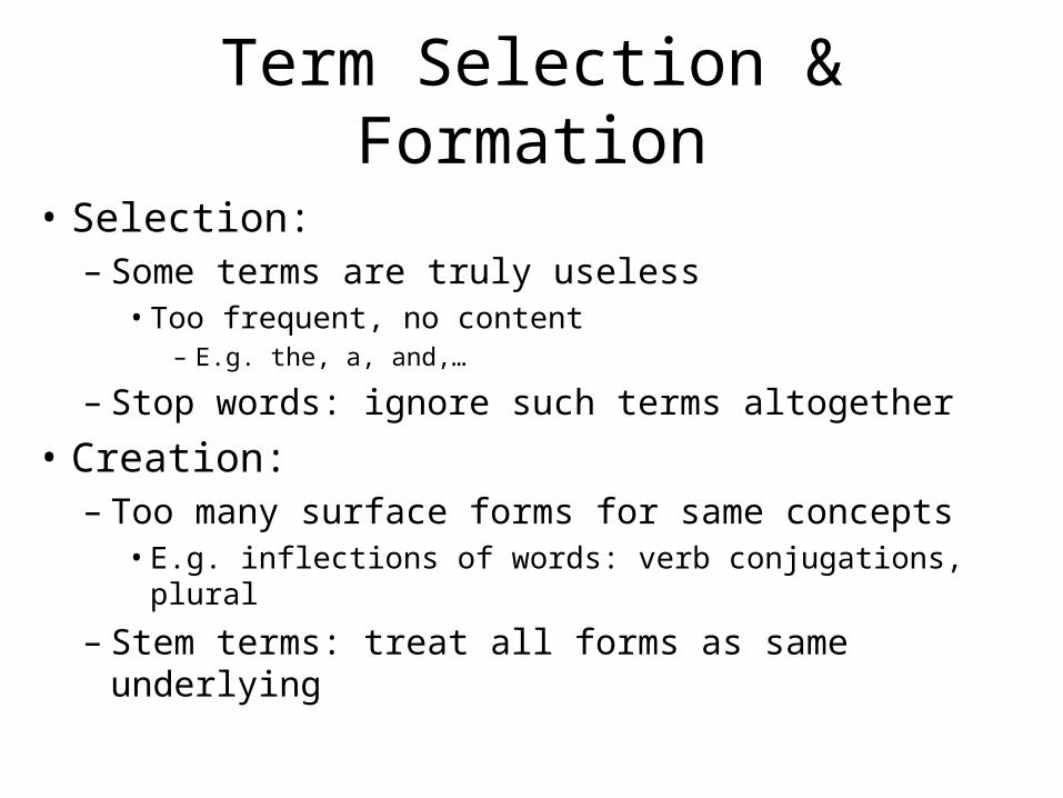
Term Selection & Formation

• Selection:– Some terms are truly useless

• Too frequent, no content– E.g. the, a, and,…

– Stop words: ignore such terms altogether

• Creation:– Too many surface forms for same concepts

• E.g. inflections of words: verb conjugations, plural

– Stem terms: treat all forms as same underlying

Key Issue

• All approaches operate on term matching– If a synonym, rather than original term, is used,

approach fails

• Develop more robust techniques– Match “concept” rather than term

• Expansion approaches– Add in related terms to enhance matching

• Mapping techniques– Associate terms to concepts

» Aspect models, stemming

Expansion Techniques

• Can apply to query or document

• Thesaurus expansion– Use linguistic resource – thesaurus, WordNet

– to add synonyms/related terms

• Feedback expansion– Add terms that “should have appeared”

• User interaction– Direct or relevance feedback

• Automatic pseudo relevance feedback

Query Refinement

• Typical queries very short, ambiguous– Cat: animal/Unix command– Add more terms to disambiguate, improve

• Relevance feedback– Retrieve with original queries– Present results

• Ask user to tag relevant/non-relevant

– “push” toward relevant vectors, away from nr

– β+γ=1 (0.75,0.25); r: rel docs, s: non-rel docs– “Roccio” expansion formula

S

kk

R

jjii sS

rR

qq11

1

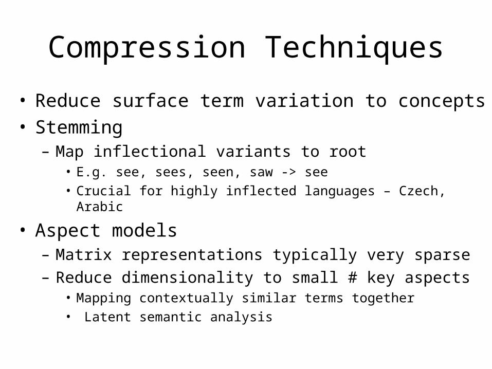
Compression Techniques

• Reduce surface term variation to concepts• Stemming

– Map inflectional variants to root• E.g. see, sees, seen, saw -> see• Crucial for highly inflected languages – Czech, Arabic

• Aspect models– Matrix representations typically very sparse– Reduce dimensionality to small # key aspects

• Mapping contextually similar terms together• Latent semantic analysis

Authoritative Sources

• Based on vector space alone, what would you expect to get searching for “search engine”?– Would you expect to get Google?

Issue

Text isn’t always best indicator of content

Example:

• “search engine” – Text search -> review of search engines

• Term doesn’t appear on search engine pages• Term probably appears on many pages that point

to many search engines

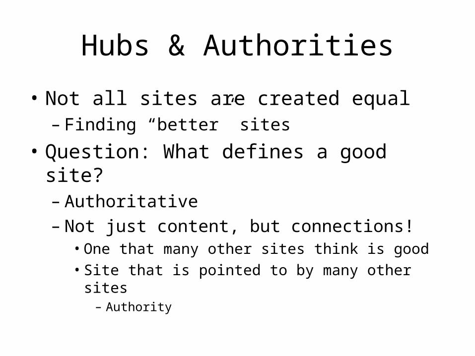
Hubs & Authorities

• Not all sites are created equal– Finding “better” sites

• Question: What defines a good site?– Authoritative– Not just content, but connections!

• One that many other sites think is good• Site that is pointed to by many other sites

– Authority

Conferring Authority

• Authorities rarely link to each other– Competition

• Hubs:– Relevant sites point to prominent sites on topic

• Often not prominent themselves• Professional or amateur

• Good Hubs Good Authorities

Computing HITS

• Finding Hubs and Authorities

• Two steps:– Sampling:

• Find potential authorities

– Weight-propagation:• Iteratively estimate best hubs and authorities

Sampling

• Identify potential hubs and authorities– Connected subsections of web

• Select root set with standard text query

• Construct base set:– All nodes pointed to by root set– All nodes that point to root set

• Drop within-domain links

– 1000-5000 pages

Weight-propagation

• Weights:– Authority weight: – Hub weight:

• All weights are relative

• Updating:

• Converges • Pages with high x: good authorities; y: good hubs

pxpy

pqqpp

pqqpp

xy

yx

,

,

Google’s PageRank

• Identifies authorities– Important pages are those pointed to by many other

pages• Better pointers, higher rank

– Ranks search results

– t:page pointing to A; C(t): number of outbound links• d:damping measure

– Actual ranking on logarithmic scale– Iterate

))(/)(...)(/)(()1()( 11 nn tCtprtCtprddApr

Contrasts

• Internal links– Large sites carry more weight

• If well-designed

– H&A ignores site-internals

• Outbound links explicitly penalized

• Lots of tweaks….

Web Search

• Search by content– Vector space model

• Word-based representation• “Aboutness” and “Surprise”• Enhancing matches• Simple learning model

• Search by structure– Authorities identified by link structure of web

• Hubs confer authority

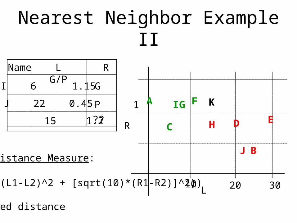
Nearest Neighbor Example II

• Credit Rating:– Classifier: Good /

Poor– Features:

• L = # late payments/yr; • R = Income/Expenses

Name L R G/P

A 0 1.2 G

B 25 0.4 P

C 5 0.7 G

D 20 0.8 PE 30 0.85 P

F 11 1.2 G

G 7 1.15 GH 15 0.8 P

Nearest Neighbor Example II

Name L R G/P

A 0 1.2 G

B 25 0.4 P

C 5 0.7 G

D 20 0.8 PE 30 0.85 P

F 11 1.2 G

G 7 1.15 GH 15 0.8 P L

R

302010

1 A

B

C D E

FG

H

Nearest Neighbor Example II

L 302010

1 A

B

C D E

FG

HR

Name L R G/P

I 6 1.15

J 22 0.45

K 15 1.2

G

IP

J

??

K

Distance Measure:

Sqrt ((L1-L2)^2 + [sqrt(10)*(R1-R2)]^2))

- Scaled distance

Efficient Implementations

• Classification cost:– Find nearest neighbor: O(n)

• Compute distance between unknown and all instances

• Compare distances

– Problematic for large data sets

• Alternative:– Use binary search to reduce to O(log n)

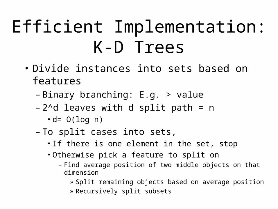
Efficient Implementation: K-D Trees

• Divide instances into sets based on features– Binary branching: E.g. > value– 2^d leaves with d split path = n

• d= O(log n)

– To split cases into sets,• If there is one element in the set, stop• Otherwise pick a feature to split on

– Find average position of two middle objects on that dimension

» Split remaining objects based on average position» Recursively split subsets

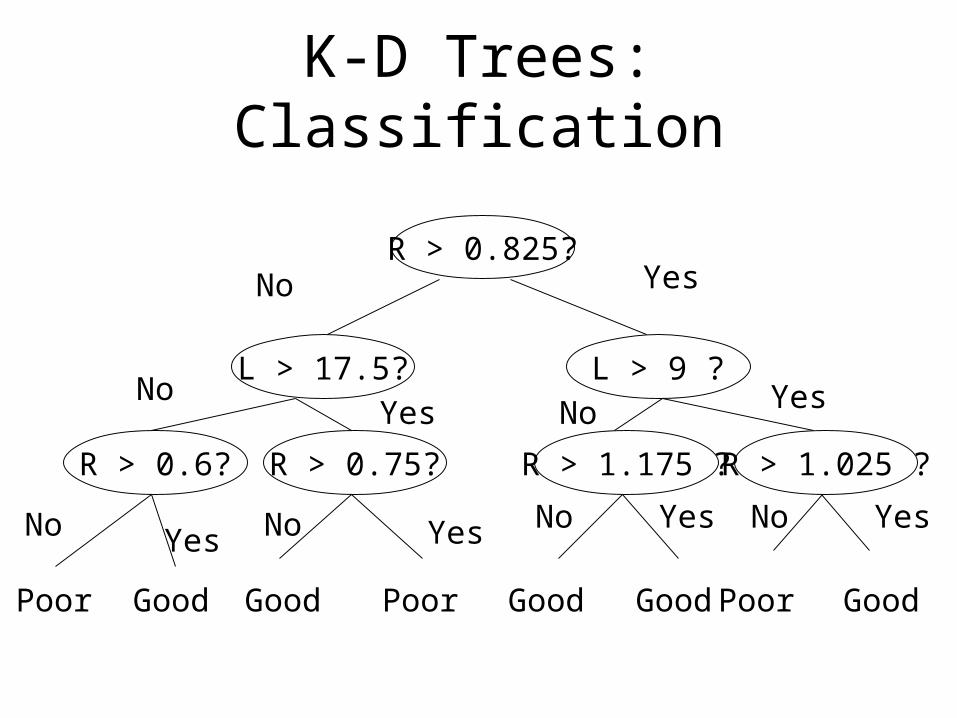
K-D Trees: Classification

R > 0.825?

L > 17.5? L > 9 ?

No Yes

R > 0.6? R > 0.75? R > 1.025 ?R > 1.175 ?

NoYes No Yes

No

Poor Good

Yes No Yes

Good Poor

No Yes

Good Good

No

Poor

Yes

Good

Efficient Implementation:Parallel Hardware

• Classification cost:– # distance computations

• Const time if O(n) processors

– Cost of finding closest• Compute pairwise minimum, successively• O(log n) time

Nearest Neighbor: Issues

• Prediction can be expensive if many features

• Affected by classification, feature noise– One entry can change prediction

• Definition of distance metric– How to combine different features

• Different types, ranges of values

• Sensitive to feature selection

Nearest Neighbor Analysis

• Problem: – Ambiguous labeling, Training Noise

• Solution:– K-nearest neighbors

• Not just single nearest instance

• Compare to K nearest neighbors– Label according to majority of K

• What should K be?– Often 3, can train as well

Nearest Neighbor: Analysis

• Issue: – What is a good distance metric?– How should features be combined?

• Strategy:– (Typically weighted) Euclidean distance– Feature scaling: Normalization

• Good starting point: – (Feature - Feature_mean)/Feature_standard_deviation– Rescales all values - Centered on 0 with std_dev 1

Nearest Neighbor: Analysis

• Issue: – What features should we use?

• E.g. Credit rating: Many possible features– Tax bracket, debt burden, retirement savings, etc..

– Nearest neighbor uses ALL – Irrelevant feature(s) could mislead

• Fundamental problem with nearest neighbor

Nearest Neighbor: Advantages

• Fast training:– Just record feature vector - output value set

• Can model wide variety of functions– Complex decision boundaries– Weak inductive bias

• Very generally applicable

Summary

• Machine learning:– Acquire function from input features to value

• Based on prior training instances

– Supervised vs Unsupervised learning• Classification and Regression

– Inductive bias: • Representation of function to learn• Complexity, Generalization, & Validation

Summary: Nearest Neighbor

• Nearest neighbor:– Training: record input vectors + output value– Prediction: closest training instance to new

data

• Efficient implementations

• Pros: fast training, very general, little bias

• Cons: distance metric (scaling), sensitivity to noise & extraneous features