Evolutionary geometry of Lagrangian structures in a transitional boundarylayerWenjie Zheng, Yue Yang, and Shiyi Chen Citation: Physics of Fluids 28, 035110 (2016); doi: 10.1063/1.4944047 View online: http://dx.doi.org/10.1063/1.4944047 View Table of Contents: http://scitation.aip.org/content/aip/journal/pof2/28/3?ver=pdfcov Published by the AIP Publishing Articles you may be interested in Enhanced instability of supersonic boundary layer using passive acoustic feedback Phys. Fluids 28, 024103 (2016); 10.1063/1.4940324 Compressible turbulent channel flow with impedance boundary conditions Phys. Fluids 27, 035107 (2015); 10.1063/1.4914099 Effects of injection on the instability of boundary layers over hypersonic configurations Phys. Fluids 25, 104107 (2013); 10.1063/1.4825038 Detuned resonances of Tollmien-Schlichting waves in an airfoil boundary layer: Experiment, theory,and direct numerical simulation Phys. Fluids 24, 094103 (2012); 10.1063/1.4751246 Fundamental and subharmonic transition to turbulence in zero-pressure-gradient flat-plateboundary layers Phys. Fluids 24, 091104 (2012); 10.1063/1.4744967

Reuse of AIP Publishing content is subject to the terms at: https://publishing.aip.org/authors/rights-and-permissions. Downloaded to IP: 123.122.36.17

On: Fri, 18 Mar 2016 17:17:24

PHYSICS OF FLUIDS 28, 035110 (2016)

Evolutionary geometry of Lagrangian structuresin a transitional boundary layer

Wenjie Zheng,1 Yue Yang,1,2,a) and Shiyi Chen1,2,31State Key Laboratory for Turbulence and Complex Systems, College of Engineering,Peking University, Beijing 100871, China2Center for Applied Physics and Technology, Peking University, Beijing 100871, China3Department of Mechanics and Aerospace Engineering, South University of Scienceand Technology of China, Shenzhen 518055, China

(Received 16 September 2015; accepted 28 February 2016; published online 18 March 2016)

We report a geometric study of Lagrangian structures in a weakly compress-ible, spatially evolving transitional boundary layer at the Mach number 0.7. TheLagrangian structures in the transition process are extracted from the Lagrangianscalar field by a sliding window filter at a sequence of reference times. The multi-scale and multi-directional geometric analysis is applied to characterize the geometryof spatially evolving Lagrangian structures, including the averaged inclination andsweep angles at different scales ranging from one half of the boundary layer thicknessto several viscous length scales. Here, the inclination angle is on the plane of thestreamwise and wall-normal directions, and the sweep angle is on the plane of thestreamwise and spanwise directions. In general, the averaged inclination angle isincreased and the sweep angle is decreased with the reference time. The variationof the angles for large-scale structures is smaller than that for small-scale structures.Before the transition, the averaged inclination and sweep angles are only slightlyaltered for all the scales. As the transition occurs, averaged inclination angles increaseand sweep angles decrease rapidly for small-scale structures. In the late transitionalstage, the averaged inclination angle of small-scale structures with 30 viscous lengthscales is approximately 42◦, and the averaged sweep angle in the logarithm lawregion is approximately 30◦. Additionally, the geometry of Lagrangian structures intransitional boundary layer flow is compared with that in the fully developed turbulentchannel flow. C 2016 AIP Publishing LLC. [http://dx.doi.org/10.1063/1.4944047]

I. INTRODUCTION

The laminar-turbulent transition of boundary layers is a fundamental and challenging problemin modern fluid mechanics. The boundary layer transition has a strong influence on aerodynamicdrag and heating because much higher friction and heating can be generated on the surface ofaerospace vehicles in turbulent flows than in laminar flows. The prediction of the transition hasan impact on the shape design and heat protection of the vehicles. Despite considerable effortsin experimental, theoretical, and numerical studies, we have not reached a consensus upon theunderlying mechanism for the formation and evolution of flow structures in the transition.1

In the transition process, there is a general agreement on the existence of coherent structuresand their importance in mixing and transport phenomena. Therefore, the detection of the coherentstructures is helpful to explain the underlying physics of transitional fluid motions and to improveturbulent flow modeling and control strategies. Qualitative discussions on the coherent structureswith different structural characteristics in the turbulent boundary layer are given in the reviews.2–4

The quasi-streamwise vortices and associated low- and high-speed streaks are mainly observed in

a)Electronic mail: yyg@pku.edu.cn

1070-6631/2016/28(3)/035110/19/$30.00 28, 035110-1 ©2016 AIP Publishing LLC

Reuse of AIP Publishing content is subject to the terms at: https://publishing.aip.org/authors/rights-and-permissions. Downloaded to IP: 123.122.36.17

On: Fri, 18 Mar 2016 17:17:24

035110-2 Zheng, Yang, and Chen Phys. Fluids 28, 035110 (2016)

the viscous sublayer and the buffer layer, while other structures in various forms, such as arches andhairpins, are populated in the logarithmic layer and the outer layer.

Although the geometry of coherent structures is of interest for structure-based models ofnear-wall turbulence,5,6 the observed geometry is strongly dependent upon structure identificationmethods. Both Eulerian criteria and Lagrangian approaches have been widely used for investigatingthe coherent structures. The Eulerian criteria, usually derived from the instantaneous velocity fieldand its gradient tensor, are widely used in experimental studies7,8 and numerical simulations9–14 toidentify the coherent structures in boundary layer flows.

On the other hand, the Lagrangian methods identify coherent structures based on the trajectoriesof fluid particles. In experiments, flow visualization employing dye,15 bubbles,16 and smoke revealedrich geometries in coherent structures, but these techniques remain mainly qualitative.3 In numericalsimulations, Green et al.17 used the direct Lyapunov exponent (DLE) to detect Lagrangian coherentstructures18 in channel flows. They concluded that the Lagrangian methods appear to be better suitedfor the investigation on the evolution of coherent structures in the transition process.

The evolution of the material surface, which is a fundamental Lagrangian structure and isuniquely defined in temporal evolution, can be tracked as the iso-surface of the Lagrangian scalarfield. This method has been applied in isotropic turbulence,19 Taylor-Green and Kida-Pelz flows,20

the K-type transition in channel flow,21 and fully developed channel flows.22 We note that theflows in the previous Lagrangian studies mentioned are incompressible, and we will extend theLagrangian method to a compressible flow.

Besides the uncertainties in the usage of different structural diagnostic tools, the accepted geom-etry of structures with a broad range of length scales in boundary layer is still far from an agreement.Theodorsen23 first proposed that incompressible turbulent boundary layers are populated by hairpin-like structures attached to the wall and inclined at 45◦. This hypothesis is experimentally supported byHead and Bandyopadhyay.24 They showed a characteristic inclination angle 40◦ − 50◦ for candidatehairpins. Using hot-wire measurements, Ong and Wallace25 achieved similar results, and they foundthat the sweep angle of vorticity vectors increased with distance from the wall. Using the particle-image velocimetry and statistical tools, Ganapathisubramani et al.8 revealed that the inclination angleis approximately equal to 45◦. Robinson26 performed both single and dual hot-wire measurements onthe large-scale structures in a supersonic boundary layer at the Mach number 2.97 and concluded thatthe inclination angle of the large-scale structures ranges from 5◦ to 30◦. Pirozzoli et al.12 found theinclination angle is approximately 20◦ in the outer layer in a supersonic boundary layer at the Machnumber 2, which is very similar to the findings in incompressible flows. Since the characterization ofthe geometry of coherent structures depends on the scale of structures, the Mach number, the Reynoldsnumber, and the usage of Eulerian or Lagrangian methods, it still remains as an open question.22

Considering the evolutionary, multi-scale nature of transitional flows, we need to develop auseful diagnostic tool characterizing evolving structures at different scales and at different statesduring the transition. In the past few years, the multi-scale decomposition has drawn attention inthe turbulence community, and has proven to be useful for understanding the evolution of coherentstructures and interactions between these structures at different scales.22,27,28 Particularly, Yangand Pullin22 developed a geometric diagnostic methodology based on the mirror-extended curvelettransform29 to characterize the multi-scale and multi-directional statistical geometry in the evolutionof Lagrangian fields in fully developed channel flows.

The major objective of the present study is to quantitatively characterize the geometric featuresof evolving structures in the transition of a weakly compressible, spatially evolving flat-plate bound-ary layer flow from a Lagrangian perspective. The backward-particle-tracking method developed inincompressible flows is extended to compressible boundary layer flows. A sliding window filter isdeveloped to extract the Lagrangian structures at different locations in the transition. Furthermore,the multi-scale and multi-directional geometric analysis is applied to characterize the evolutionarygeometry of Lagrangian structures within the sliding window. This provides quantitative statisticson the orientation of turbulent structures at different scales and locations in the streamwise direc-tion. Flow phenomena in transitional wall flows to be investigated are based on statistical evidenceobtained from the geometric analysis, including the detailed geometry of quasi-streamwise vorticesand the generation and evolution of near-wall vortical structures.

Reuse of AIP Publishing content is subject to the terms at: https://publishing.aip.org/authors/rights-and-permissions. Downloaded to IP: 123.122.36.17

On: Fri, 18 Mar 2016 17:17:24

035110-3 Zheng, Yang, and Chen Phys. Fluids 28, 035110 (2016)

We begin in Sec. II as an overview of numerical implementations for the direct numerical simu-lation (DNS) of the compressible boundary layer and the tracking of the Lagrangian scalar field. InSec. III, a diagnostic methodology is introduced, including the characterization of the geometry ofLagrangian structures at multiple scales and the extraction of Lagrangian structures with a slidingwindow filter. Sec. IV presents the application of the multi-scale and multi-directional diagnosticmethod to investigate the evolutionary geometry of Lagrangian structures in the transition. Finally,we draw some conclusions in Sec. V.

II. SIMULATION OVERVIEW

A. DNS

The DNS of a spatially evolving flat-plate boundary layer transition in the domain with sizesLx × Ly × Lz (see Fig. 1) is performed by solving the three-dimensional compressible Navier–Stokes(N–S) equations,

∂U∂t+∂F j

∂x j−∂V j

∂x j= 0, (1)

where

U =

*........,

ρ

ρu1

ρu2

ρu3

E

+////////-

, F j =

*........,

ρu j

ρu1u j + pδ1 j

ρu2u j + pδ2 j

ρu3u j + pδ3 j

(E + p)u j

+////////-

, V j =

*..........,

0σ1 j

σ2 j

σ3 j

σ jkuk + κ∂T∂x j

+//////////-

. (2)

Here, the Einstein summation is used, and the subscript j = 1,2,3 denotes the index in the three-dimensional Cartesian coordinates. For the coordinate system shown in Fig. 1, x1, x2, and x3 areequivalent to x, y , and z, respectively. The velocity components are denoted by variables u j in thejth coordinate direction, or u, v , and w in the x, y , and z directions, respectively, ρ is the density, pis the static pressure, δi j is the Kronecker delta function, κ is the thermal conductivity, and T is thetemperature. The N–S equations Eq. (1) are nondimensionalized with the free stream quantities ρ∞,T∞, U∞, and µ∞. The length and time scales are nondimensionalized by the reference length L = 1inch and time L/U∞, respectively. In the perfect gas assumption, the total energy E is given by

E = ρcvT + ρuiui/2, (3)

where cv is the specific heat at constant volume. For compressible Newtonian flow, the viscousstress σi j can be written as

σi j = µ

(∂ui

∂x j+∂u j

∂xi

)− 2

3µ∂uk

∂xkδi j, (4)

where the dynamic viscosity µ is assumed to obey Sutherland’s law.

FIG. 1. A schematic diagram of the computational domain and the characteristic angles of structures. Possible structures aresketched by dashed lines.

Reuse of AIP Publishing content is subject to the terms at: https://publishing.aip.org/authors/rights-and-permissions. Downloaded to IP: 123.122.36.17

On: Fri, 18 Mar 2016 17:17:24

035110-4 Zheng, Yang, and Chen Phys. Fluids 28, 035110 (2016)

The computational domain is bounded by an inlet boundary and a non-reflecting outflowboundary in the streamwise x-direction, a wall boundary and a non-reflecting upper boundary inthe wall-normal y-direction, and two periodic boundaries in the spanwise z-direction. The wall isisothermal, and the physical boundary condition of the velocity on the flat-plate is the no-slip condi-tion. The initial condition is given by a laminar compressible boundary-layer similarity solution. Inorder to trigger the laminar-to-turbulent transition, a two-dimensional Tollmien–Schlichting (T–S)wave and a couple of conjugate three-dimensional T–S waves are imposed at the inlet. Then theinlet boundary condition can be written as

f (y, z) = f L(y) +3j=1

ε j f j(y)ei(β jz−ω j t) (5)

with f = (ρ,u, v,w,T)T. Here, f L(y) is the steady flow profile obtained from the self-similar solu-tion30 of the compressible laminar boundary layer over the flat-plate at x = 30. Moreover, theamplitudes of these disturbances are ε1 = 0.04 and ε2 = ε3 = 0.001, the spanwise wavenumbersare β1 = 0, β2 = 4.0, and β3 = −4.0, the frequency is ω j = 1.56, and f j are the eigenfunctionscorresponding to these three T–S waves. These T–S wave parameters are obtained by solving theOrr–Sommerfeld equation using a Chebyshev spectral collocation method.31 The spanwise wave-length of the three-dimensional T–S waves is λz = 2π/β2 = 1.57, the period of the T–S waves isτTS = 2π/ω j = 4.0, the real part of the phase velocity is cr = 0.35, and the streamwise wavelength isλx = crτTS = 1.4.

The DNS is implemented using the OpenCFD code.32 The N–S equations Eq. (1) are inte-grated in time by using the third-order TV Runge–Kutta method. The convection terms ∂F j/∂x j areapproximated by a seventh-order upwind finite-difference scheme, and the viscous terms ∂V j/∂x j

are approximated by an eighth-order central finite-difference scheme.Grid A (see Table I) employed in the present simulation was selected through a grid sensitivity

analysis. Three grids were considered, and their parameters are listed in Table I. The subscript“∞” denotes the free stream properties, and “w” denotes the quantities on the wall. The freestream Mach number is Ma∞ ≡ U∞/c∞ = 0.7 where c∞ is the free stream sound speed. The DNSof the transitional boundary layer at Ma∞ = 0.7 was validated with experimental results,33 and thecompressibility effects on the evolution of coherent structures is weak at this Mach number.34 Thefree stream Reynolds number is Re∞ ≡ ρ∞U∞L/µ∞, and the wall temperature Tw is normalized bythe free stream temperature T∞ = 288.15 K. It is noted the width Lz in the spanwise direction isequal to the spanwise wavelength λz of the T–S waves. The two-point correlations of the velocitycomponents in the spanwise direction were calculated. We found that the tails of the two-pointcorrelations are sufficiently small at the boundary (not shown), which ensures that Lz is largeenough so that the imposed periodic boundary condition is not affecting the flow statistics.35

The domain is discretized using grids Nx × Ny × Nz. Uniform grids are distributed in thestreamwise and spanwise directions with grid spacings ∆x and ∆z. Exponentially stretched gridswith grid points at

y j = Lyep( j−1)/(Ny−1) − 1

ep − 1, j = 1,2, . . . ,Ny,

where p = log q/(1 − 1/Ny) and q = 53, were applied in the wall-normal direction with grid spac-ing ∆y to capture small-scale structures near the wall. The superscript “+” denotes the quantitiesnormalized by wall units,3 which are defined in terms of the viscous length scale δν ≡ µw/(ρwuτ)and the friction velocity uτ ≡

τw/ρw with the wall shear stress τw. The wall-friction Reynolds

TABLE I. DNS parameters.

Grids Ma∞ Re∞ Tw Lx×L y×Lz Nx×Ny×Nz ∆x+×∆y+w×∆z+

A 0.7 50 000 1.098 10.00 × 0.65 × 1.57 2000 × 100 × 640 10.07 × 0.98 × 4.94B 0.7 50 000 1.098 10.00 × 0.65 × 1.57 1000 × 100 × 320 19.96 × 0.97 × 9.78C 0.7 50 000 1.098 10.00 × 0.65 × 1.57 4000 × 100 × 640 5.07 × 0.98 × 4.98

Reuse of AIP Publishing content is subject to the terms at: https://publishing.aip.org/authors/rights-and-permissions. Downloaded to IP: 123.122.36.17

On: Fri, 18 Mar 2016 17:17:24

035110-5 Zheng, Yang, and Chen Phys. Fluids 28, 035110 (2016)

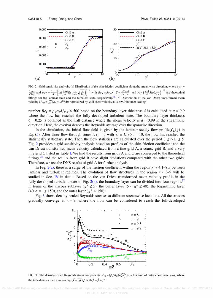
FIG. 2. Grid sensitivity analysis. (a) Distribution of the skin-friction coefficient along the streamwise direction, where c f L =

0.664√Rex

and c f T =0.455S2

ln

(0.06S Rex 1

µw

1Tw

)−2with Rex ≡Re∞x, S =

√Tw−1

sin−1A, and A=

(γ−1

2 Ma2∞

1Tw

)1/2are theoretical

fittings for the laminar state and the turbulent state, respectively.36 (b) Distribution of the van Driest transformed meanvelocity Uvd =

u0 (ρ/ρw)1/2du normalized by wall shear velocity at x = 9.9 in inner scaling.

number Reτ ≡ ρwuτδ/µw ≈ 500 based on the boundary layer thickness δ is calculated at x = 9.9where the flow has reached the fully developed turbulent state. The boundary layer thicknessδ = 0.25 is obtained as the wall distance where the mean velocity is u = 0.99 in the streamwisedirection. Here, the overbar denotes the Reynolds average over the spanwise direction.

In the simulation, the initial flow field is given by the laminar steady flow profile f L(y) inEq. (5). After three flow-through times t/τx = 3 with τx ≡ Lx/U∞ = 10, the flow has reached thestatistically stationary state. Then the flow statistics are calculated over the period 3 ≤ t/τx ≤ 5.Fig. 2 provides a grid sensitivity analysis based on profiles of the skin-friction coefficient and thevan Driest transformed mean velocity calculated from a fine grid A, a coarse grid B, and a veryfine grid C listed in Table I. We find the results from grids A and C are converged to the theoreticalfittings,36 and the results from grid B have slight deviations compared with the other two grids.Therefore, we use the DNS results of grid A for further analysis.

In Fig. 2(a), there is a surge of the friction coefficient within the region x ≈ 4.1–8.5 betweenlaminar and turbulent regimes. The evolution of flow structures in the region x ≈ 3–9 will bestudied in Sec. IV in detail. Based on the van Driest transformed mean velocity profile in thefully developed turbulent state in Fig. 2(b), the boundary layer can be divided into four regions37

in terms of the viscous sublayer (y+ ≤ 5), the buffer layer (5 < y+ ≤ 40), the logarithmic layer(40 < y+ ≤ 150), and the outer layer (y+ > 150).

Fig. 3 shows density-scaled Reynolds stresses at different streamwise locations. All the stressesgradually converge at x = 9, where the flow can be considered to reach the full-developed

FIG. 3. The density-scaled Reynolds stress components Ri j = (ρ/ρw)u′′i u′′j as a function of outer coordinate y/δ, where

the tilde denotes the Favre average f = ρ f /ρ with f = f + f ′′.

Reuse of AIP Publishing content is subject to the terms at: https://publishing.aip.org/authors/rights-and-permissions. Downloaded to IP: 123.122.36.17

On: Fri, 18 Mar 2016 17:17:24

035110-6 Zheng, Yang, and Chen Phys. Fluids 28, 035110 (2016)

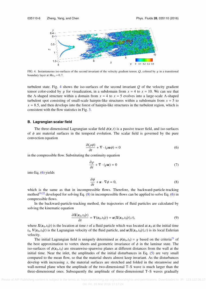
FIG. 4. Instantaneous iso-surfaces of the second invariant of the velocity gradient tensor, Q, colored by y in a transitionalboundary layer at Ma∞= 0.7.

turbulent state. Fig. 4 shows the iso-surfaces of the second invariant Q of the velocity gradienttensor color-coded by y for visualization, in a subdomain from x = 4 to x = 10. We can see thatthe Λ-shaped structure within a domain from x = 4 to x = 5 evolves into a large-scale Λ-shapedturbulent spot consisting of small-scale hairpin-like structures within a subdomain from x = 5 tox = 8.5, and then develops into the forest of hairpin-like structures in the turbulent region, which isconsistent with the flow statistics in Fig. 3.

B. Lagrangian scalar field

The three-dimensional Lagrangian scalar field φ(x, t) is a passive tracer field, and iso-surfacesof φ are material surfaces in the temporal evolution. The scalar field is governed by the pureconvection equation

∂(ρφ)∂t+ ∇ · (ρuφ) = 0 (6)

in the compressible flow. Substituting the continuity equation

∂ρ

∂t+ ∇ · (ρu) = 0 (7)

into Eq. (6) yields

∂φ

∂t+ u · ∇φ = 0, (8)

which is the same as that in incompressible flows. Therefore, the backward-particle-trackingmethod19,22 developed for solving Eq. (8) in incompressible flows can be applied to solve Eq. (6) incompressible flows.

In the backward-particle-tracking method, the trajectories of fluid particles are calculated bysolving the kinematic equation

∂X(x0, t0|t)∂t

= V(x0, t0|t) = u(X(x0, t0|t), t), (9)

where X(x0, t0|t) is the location at time t of a fluid particle which was located at x0 at the initial timet0, V(x0, t0|t) is the Lagrangian velocity of the fluid particle, and u(X(x0, t0|t), t) is its local Eulerianvelocity.

The initial Lagrangian field is uniquely determined as φ(x0, t0) = y based on the criteria21 ofthe best approximation to vortex sheets and geometric invariance of φ in the laminar state. Theiso-surfaces of φ(x0, t0) are streamwise-spanwise planes at different distances from the wall at theinitial time. Near the inlet, the amplitudes of the initial disturbances in Eq. (5) are very smallcompared to the mean flow, so that the material sheets almost keep invariant. As the disturbancesdevelop with increasing x, the material surfaces are stretched and folded in the streamwise andwall-normal plane when the amplitude of the two-dimensional T–S wave is much larger than thethree-dimensional ones. Subsequently the amplitude of three-dimensional T–S waves gradually

Reuse of AIP Publishing content is subject to the terms at: https://publishing.aip.org/authors/rights-and-permissions. Downloaded to IP: 123.122.36.17

On: Fri, 18 Mar 2016 17:17:24

035110-7 Zheng, Yang, and Chen Phys. Fluids 28, 035110 (2016)

FIG. 5. A schematic diagram of backward particle-tracking in a transitional boundary layer.

becomes notable with growing disturbances. As a result, the material surfaces can be rolled up intocomplex shapes with three-dimensional geometric characteristics in the evolution.21

The backward-particle-tracking method19 is numerically stable and has no numerical dissipa-tion, which can ensure the mass conservation within a closed material surface. In the numericalimplementation, this method is used to calculate the Lagrangian scalar field at different givenphysical times as follows.

(1) The full Eulerian velocity field on the grids Nx × Ny × Nz within a time interval from t0 tot > t0 is solved by DNS described in Sec. II A and then stored in disk. The time step isselected by ∆t ≤ δν/uτ to capture the finest resolved scales in the velocity field.

(2) At a given time t, particles are placed at the uniform grid points of N px × N p

y × N pz in the

subdomain of interest for further geometric analysis. In principle, the time interval ∆T ≡ t − t0for backward particle-tracking should be selected to ensure that all the particles at the outletboundary xout of the subdomain can travel backward to the inlet location x = 0, but in thespatially developed wall flows, it can take very long time for the particles very close to thewall traveling back to x0 owing to the very small streamwise velocity. In the implementation,we set ∆T = (xout − xin)/U∞ to greatly reduce the computational cost with negligible devi-ations, where xin is the location for the inlet boundary of the subdomain. The diagram ofbackward particle-tracking during ∆T is shown in Fig. 5. We find that the statistical resultsare not sensitive to the value of ∆T for ∆T ≥ (xout − xin)/U∞ from numerical experiments. Forexample, in a subdomain of interest from xin = 3.0 to xout = 9.0, we can obtain φ(x, t) at aparticular time t = t∗ where t∗ ≡ t0 + ∆T = 36 at the end of the tracking period with t0 = 3τx.

(3) The particles are released and their trajectories are calculated backward in time within ∆T oruntil they arrive at x0 = 1.0, where the initial disturbances are small enough so that the initialmaterial surfaces are considered as flat sheets. A three-dimensional, fourth-order Lagrangianinterpolation scheme is used to obtain fluid velocity at the location of each particle, and anexplicit, second-order Adams-Bashforth scheme is applied for the time integration.

(4) After the backward tracking, we can obtain initial locations x0 of the particles and the flowmap

F t0t (X) : X(x0, t0|t) → x0, t ≥ t0. (10)

Then the Lagrangian field φ(x, t) at any given time t can be obtained as

φ(x, t) = φ(F t0t (X) , t0) = φ(x0, t0). (11)

III. DIAGNOSTIC METHODOLOGIES

A. Multi-scale and multi-directional decomposition

Although different characteristic scales and preferred orientations of flow structures via variousstructural identification methods have been reported, there is lack of quantified consensus on thegeometry of the structures. The geometric feature of characteristic scales and preferred orientationsin a scalar field can be quantified by the multi-scale and multi-directional methodology22 based on

Reuse of AIP Publishing content is subject to the terms at: https://publishing.aip.org/authors/rights-and-permissions. Downloaded to IP: 123.122.36.17

On: Fri, 18 Mar 2016 17:17:24

035110-8 Zheng, Yang, and Chen Phys. Fluids 28, 035110 (2016)

TABLE II. Characteristic length scales Lj normalized by the boundary layer thickness δ and viscous length scale δν atx = 9.9.

Length Scale 1 Scale 2 Scale 3 Scale 4 Scale 5 Scale 6 Scale 7 Scale 8 Scale 9

Lj/δ 2 1 0.5 0.25 0.125 0.0625 0.0313 0.0156 0.0078Lj/δν 1000 500 250 125 62.5 31.25 15.63 7.81 3.91

the curvelet transform.29 Presently, in order to quantify geometries of flow structures at multiplescales in a three-dimensional field, we apply the multi-scale and multi-directional filter to typicaltwo-dimensional x–y and x–z plane-cuts.

The Fourier transform of an arbitrary two-dimensional scalar field ϕ ∈ R2 is defined by

ϕ(k) = 12π

R

ϕ(x)e−ik·xdx. (12)

Then a filtered ϕ(x) at the scale j and along the direction l can be extracted from ϕ(k) in Fourierspace by the frequency window function

Uj(r, θ) = 2−3 j/4W (2− jr)V (tl(θ)) (13)

with r =

k21 + k2

2 and θ = arctan(k2/k1). Here, W (r) is the radial window function and V (tl) is

the angular window function, which are defined by explicit functions.22 Each frequency windowfunction in Fourier space is supported on a region bounded by two neighbouring circular wedges inthe range of wavenumbers 2 j−1 ≤ r ≤ 2 j+1, which implies that the corresponding spatial structurein physical space is a needle-shaped element or a curvelet29 with the character length 2− j/2 andwidth 2− j.

By applying frequency window function Eq. (13), geometric features of a two-dimensionalscalar field can be extracted at a characteristic length scale Lj = 2− j, j ∈ N0 and an equispacedsequence of rotation angles θ j,l = πl2−⌈ j/2⌉/2,0 6 l 6 4 · 2⌈ j/2⌉ − 1, where ⌈x⌉ gives the smallestinteger greater than or equal to x. The breakdown of the normalized characteristic length scales ofstructures after filtering is given in Table II. Subsequently, Lj ≥ 0.5δ will be referred to as “largescale,” Lj ≤ 100δν as “small scale,” and in between as “intermediate scale.”

For each scale j, the multi-scale decomposition of the original scalar field ϕ(x) can be obtainedby applying the radial window function W (r) as a band-pass filter on ϕ(k) as

ϕ j(x) =

ϕ(k)W (2− jr)eik·xdk, (14)

where ϕ j(x) is the filtered component field at scale j. The structures educed for each filtered scalehave a correspondence with the different compact energetic bands in Fourier space.

Furthermore, the orientation information of ϕ(x) can be represented by the normalized angularspectrum

Φ j(∆θ) =ϕ(k)Uj(r, θ)dk

Uj(r, θ)dk, −π

26 ∆θ 6

π

2, (15)

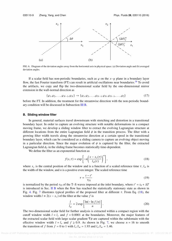
where ∆θ = πl ′2−⌈ j/2⌉/2, −2⌈ j/2⌉ 6 l ′ 6 2⌈ j/2⌉ is the discrete deviation angle away from the hori-zontal axis in the physical space, as sketched in Fig. 6(a) for scale j.

The averaged deviation angles away from the horizontal axis, which are sketched in Fig. 6(b),can be obtained by

⟨∆θ⟩+j =l′max

l′=0Φ j(∆θ)∆θl′maxl′=0Φ j(∆θ)

and ⟨∆θ⟩−j =0

l′=l′minΦ j(∆θ)∆θ0

l′=l′minΦ j(∆θ)

(16)

with l ′min = −2⌈ j/2⌉ and l ′max = 2⌈ j/2⌉.

Reuse of AIP Publishing content is subject to the terms at: https://publishing.aip.org/authors/rights-and-permissions. Downloaded to IP: 123.122.36.17

On: Fri, 18 Mar 2016 17:17:24

035110-9 Zheng, Yang, and Chen Phys. Fluids 28, 035110 (2016)

FIG. 6. Diagram of the deviation angles away from the horizontal axis in physical space. (a) Deviation angle and (b) averageddeviation angles.

If a scalar field has non-periodic boundaries, such as ϕ on the x–y plane in a boundary layerflow, the fast Fourier transform (FT) can result in artificial oscillations near boundaries.38 To avoidthe artifacts, we copy and flip the two-dimensional scalar field by the one-dimensional mirrorextension in the wall-normal direction as

{ϕ1, ϕ2, . . . , ϕN−1, ϕN} → {ϕ1, ϕ2, . . . , ϕN−1, ϕN , ϕN−1, . . . , ϕ2} (17)

before the FT. In addition, the treatment for the streamwise direction with the non-periodic bound-ary condition will be discussed in Subsection III B.

B. Sliding window filter

In general, material surfaces travel downstream with stretching and distortion in a transitionalboundary layer. In order to capture an evolving structure with notable deformations in a compactmoving frame, we develop a sliding window filter to extract the evolving Lagrangian structure atdifferent locations from the entire Lagrangian field φ in the transition process. The filter with agrowing filter width travels along the streamwise direction at a certain speed in the transitionalboundary layer, which can be considered as a sliding camera to capture an evolving object movingin a particular direction. Since the major evolution of φ is captured by the filter, the extractedLagrangian field φ f in the sliding frame becomes statistically time-dependent.

We define the filter as an exponential function as

f (x, τ) = exp−n

(x − xc(τ)

lw(τ))n

, (18)

where xc is the central position of the window and is a function of a scaled reference time τ, lw isthe width of the window, and n is a positive even integer. The scaled reference time

τ =t − t∗

τTS(19)

is normalized by the period τTS of the T–S waves imposed at the inlet boundary, where t∗ = t0 + ∆Tis introduced in Sec. II B when the flow has reached the statistically stationary state as shown inFig. 4. Fig. 7 illustrates typical profiles of the proposed filter at different τ. From Eq. (18), thewindow width l ≡ 2(x − xc) of the filter at the value f is

llw= 2 exp

ln(− ln f /n)

n

. (20)

The two-dimensional scalar field for further analysis is extracted within a compact region with thecutoff window width l = lc and f = 0.0001 at the boundaries. Moreover, the major features ofthe extracted scalar field with large scalar gradient ∇φ are captured within the subdomain with theeffective window width l = le and f ≥ 0.9. As shown in Fig. 7, we choose n = 16 to smooththe transition of f from f = 0 to 1 with lc/lw = 1.93 and le/lw = 1.46.

Reuse of AIP Publishing content is subject to the terms at: https://publishing.aip.org/authors/rights-and-permissions. Downloaded to IP: 123.122.36.17

On: Fri, 18 Mar 2016 17:17:24

035110-10 Zheng, Yang, and Chen Phys. Fluids 28, 035110 (2016)

FIG. 7. Profiles of the sliding window function at three scaled reference times τ = 0.5,1.5,2.5 to extract three φ f from theentire φ at t = t∗+2.

Since the streamwise wavelength of the T–S waves is λx = 1.4, the subdomain from x = 3 tox = 9 contains 4.3 times of λx. Considering the effects of turbulent straining, the perturbation wavesare stretched when travelling downstream. Moreover, inspired from Fig. 4, in one realization, theLagrangian scalar field φ at a physical time instant t can be spatially divided into three regions asillustrated in Fig. 7. In the implementation, we extract three different filtered scalar fields φ f at threescaled reference times τ, τ + 1, and τ + 2 from φ(x, t) at one physical time t instead of three timest, t + τTS, and t + 2τTS in principle to reduce the computational cost, considering the downstreamportion at τ + 1 is evolved from the corresponding upstream portion at τ during the time period τTS.In each realization, we investigate φ f at nine reference times τ = 0,0.25,0.5, . . . ,2.0, and they areextracted from the entire φ-data at four physical times t(m) = t∗ + m, m = 0,1,2,3. Furthermore, thegeometric statistics at different reference times are averaged over three realizations at t(m), t(m) + τTS,and t(m) + 2τTS to reduce statistical errors.

As the Lagrangian structure moving downstream in the flow evolution, the fluid is convectedat different speeds depending on the distance to the wall, which implies that the characteristic scaleof the evolving structure can be widened in the streamwise direction. Thus the sliding window isexpanded as it moves downstream by increasing lw and xc with the scaled reference time τ. Itis noted that xc(τ) and lw(τ) are fitted by quadratic polynomials from the DNS data of the threerealizations. These polynomials for the different structures studied in Sec. IV are listed in Table III,and the empirical parameters in the polynomials are chosen to ensure the major deformation ofLagrangian structures can be captured within the compact sliding window with large enough le.

With given xc(τ) and lw(τ), the extracted Lagrangian scalar field φ f (x, τ) can be obtained as

φ f (x, τ) = φ(x, t) f + φ(x0, t0)(1 − f ). (21)

The extracted Lagrangian field in the sliding window has a smooth transition from an evolvingscalar φ(x, t) to the initial scalar φ(x0, t0) at window boundaries. Thus, the boundary condition of thewindow in the streamwise direction can be considered as periodic for FT.

As an example, the temporal evolution of the material surface extracted by a sliding windowfilter with the parameters listed in Table III is shown in Fig. 8. The resolution for the Lagrangianfield is 2400 × 200 × 2560 within the subdomain of interest 3.0 6 x 6 6.0, 0 6 y 6 0.32, and

TABLE III. Empirical parameters in the central location of the sliding window filter.

Tracking structure xc(τ) lw(τ)Iso-surface of φ+= 120 0.52τ2+0.63τ+3.4 −0.53τ2+1.15τ+0.39φ on the x–y plane-cut at z = Lz/2 0.55τ2+1.05τ+3.0 0.34τ2+0.07τ+0.27φ on the x–z plane-cuts at y+= 5,30,60,120 0.15τ2+1.36τ+3.0 0.12τ2+0.25τ+0.27

Reuse of AIP Publishing content is subject to the terms at: https://publishing.aip.org/authors/rights-and-permissions. Downloaded to IP: 123.122.36.17

On: Fri, 18 Mar 2016 17:17:24

035110-11 Zheng, Yang, and Chen Phys. Fluids 28, 035110 (2016)

FIG. 8. Evolution of the material surface as the iso-surface of φ+= 120 or φ = 0.06 in a transitional boundary layer atMa∞= 0.7. It is color coded by the wall distance y. (a) τ = 0.5, (b) τ = 0.75, (c) τ = 1, (d) τ = 1.25.

0 6 z 6 1.57, which is four times that of the velocity field in order to resolve fine-scale Lagrangianstructures in the evolution.19 Fig. 8 illustrates the evolution of a material surface from the regionx ≈ 3.3–4.4 in Fig. 8(a) to the region x ≈ 4.4–5.8 downstream in Fig. 8(d) during a period of τTS.The material surface evolves from the streamwise-spanwise plane at y+ = 120. First, the planarsurface is folded owing to the two-dimensional disturbance and the mean shear motion at τ = 0.5in Fig. 8(a). Subsequently with the growth of the three-dimensional disturbance, it evolves into alarge-scale Λ-shaped bulge at τ = 0.75 in Fig. 8(b). The head of the Λ-shaped bulge is lifted atτ = 1 in Fig. 8(c), and then it is stretched and distorted into a hairpin-like structure with manysmall-scale parts at τ = 1.25 in Fig. 8(d). This evolution is qualitatively similar to the observationon material surfaces in incompressible temporal transitional channel flow,21 which suggests that thecompressibility effect at Ma∞ = 0.7 appears to be negligible on the structural evolution.

IV. EVOLUTIONARY GEOMETRY OF LAGRANGIAN STRUCTURES

A. Lagrangian structures on the streamwise and wall-normal (x–y ) plane

In a spatially developed boundary layer, we develop a sliding window filter to extract filteredLagrangian fields φ f (x, τ) at a sequence of non-dimensional reference times τ from the entireLagrangian field φ(x, t), and the Lagrangian structures for investigations are educed as iso-surfacesof φ f . The x–y plane-cuts are selected at the midpoint of Lz to show the evolution of structureswith the most significant deformation on the “peak plane.”39 The resolution of φ is 9600 × 720within the subdomain of interest 3.0 6 x 6 9.0 and 0 6 y 6 0.6. Typical snapshots of φ f on thex–y plane-cuts at different τ and corresponding spatial regions are shown in Fig. 9 to provide

FIG. 9. Typical snapshots in the evolution of the Lagrangian field on the x–y plane (0 6 y 6 0.6, z = Lz/2) in a transitionalboundary layer at Ma∞= 0.7.

Reuse of AIP Publishing content is subject to the terms at: https://publishing.aip.org/authors/rights-and-permissions. Downloaded to IP: 123.122.36.17

On: Fri, 18 Mar 2016 17:17:24

035110-12 Zheng, Yang, and Chen Phys. Fluids 28, 035110 (2016)

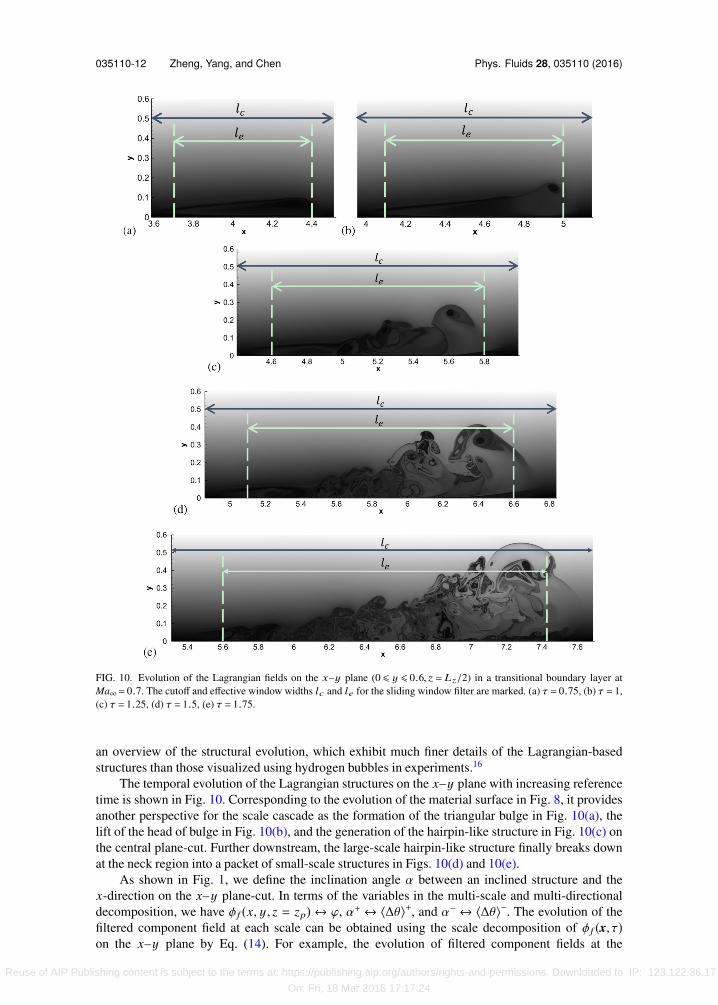
FIG. 10. Evolution of the Lagrangian fields on the x–y plane (0 6 y 6 0.6, z = Lz/2) in a transitional boundary layer atMa∞= 0.7. The cutoff and effective window widths lc and le for the sliding window filter are marked. (a) τ = 0.75, (b) τ = 1,(c) τ = 1.25, (d) τ = 1.5, (e) τ = 1.75.

an overview of the structural evolution, which exhibit much finer details of the Lagrangian-basedstructures than those visualized using hydrogen bubbles in experiments.16

The temporal evolution of the Lagrangian structures on the x–y plane with increasing referencetime is shown in Fig. 10. Corresponding to the evolution of the material surface in Fig. 8, it providesanother perspective for the scale cascade as the formation of the triangular bulge in Fig. 10(a), thelift of the head of bulge in Fig. 10(b), and the generation of the hairpin-like structure in Fig. 10(c) onthe central plane-cut. Further downstream, the large-scale hairpin-like structure finally breaks downat the neck region into a packet of small-scale structures in Figs. 10(d) and 10(e).

As shown in Fig. 1, we define the inclination angle α between an inclined structure and thex-direction on the x–y plane-cut. In terms of the variables in the multi-scale and multi-directionaldecomposition, we have φ f (x, y, z = zp)↔ ϕ, α+↔ ⟨∆θ⟩+, and α−↔ ⟨∆θ⟩−. The evolution of thefiltered component field at each scale can be obtained using the scale decomposition of φ f (x, τ)on the x–y plane by Eq. (14). For example, the evolution of filtered component fields at the

Reuse of AIP Publishing content is subject to the terms at: https://publishing.aip.org/authors/rights-and-permissions. Downloaded to IP: 123.122.36.17

On: Fri, 18 Mar 2016 17:17:24

035110-13 Zheng, Yang, and Chen Phys. Fluids 28, 035110 (2016)

FIG. 11. Evolution of the filtered component fields at scale 4 on the x–y plane (0 6 y 6 0.6, z = Lz/2) in a transitionalboundary layer at Ma∞= 0.7. Averaged inclination angles are sketched in dashed lines. (a) τ = 0.75, (b) τ = 1, (c) τ = 1.25,(d) τ = 1.5, (e) τ = 1.75.

intermediate scale with j = 4 and at the small scale with j = 6 are shown in Figs. 11 and 12,respectively. The characteristic length scale for each scale index j is quantified in Table II. Wefind that the filtered component fields at different scales show different preferential orientations.The orientation statistics of φ f (x, τ) on the x–y plane at different scales can be obtained by thenormalized angular spectra Φ j(∆θ) defined by Eq. (15), which are shown in Fig. 13 at τ = 1 andτ = 1.75. The magnitudes of angular spectra at scales j ≥ 3 are increased with time, which suggestsa structural cascade from large scales to small scales for φ f (x, τ).

It is noted that the filtered component fields at very small scales with very small angularspectrum Φ j(∆θ) < 10−8 are considered to have negligible contribution to the spectrum of φ or tobe numerical artifacts due to the weak Gibbs phenomenon from the filtering of window boundariesin Fig. 7. Moreover, the sizes of the subdomain of interest should be larger than the characteristiclength scales Lj in Table II, otherwise the filter window size can exceed the subdomain. Addition-ally, we found that the statistical geometric results from the filtered component fields with the scaleindices j ≥ 6 are qualitatively very similar to the time-averaged angle deviations less than 5◦ (notshown). Thus, we only investigate the filtered component fields with the smallest scale index j = 3to ensure the corresponding Lj can be captured in the subdomain of interest and the largest scaleindex j = 6 with Φ j(∆θ) ≥ 10−8 in the evolution.

The averaged inclination angle is defined as ⟨α⟩ = (⟨α+⟩ + ⟨α−⟩)/2. Moreover, an additionalaveraging on ⟨α⟩ was applied from three realizations to reduce statistical errors, where each real-ization is within a time interval of 2τTS. Fig. 14 shows the temporal evolution of ⟨α⟩ for filteredcomponent fields from large to small scales. The averaged inclination angle ⟨α⟩ in Fig. 14 is markedby dashed lines in Figs. 11 and 12, which depict the increasing of ⟨α⟩ during the evolution for bothscales. As shown in Fig. 12(a), the small-scale structures with small ⟨α⟩ appear at early times, andthen the small-scale structures are lifted in Figs. 12(b)–12(e).

FIG. 12. Evolution of the filtered component fields at scale 6 on the x–y plane (0 6 y 6 0.6, z = Lz/2) in a transitionalboundary layer at Ma∞= 0.7. Averaged inclination angles are sketched in dashed lines. (a) τ = 0.75, (b) τ = 1, (c) τ = 1.25,(d) τ = 1.5, (e) τ = 1.75.

Reuse of AIP Publishing content is subject to the terms at: https://publishing.aip.org/authors/rights-and-permissions. Downloaded to IP: 123.122.36.17

On: Fri, 18 Mar 2016 17:17:24

035110-14 Zheng, Yang, and Chen Phys. Fluids 28, 035110 (2016)

FIG. 13. Angular spectra of filtered component fields at different scales on the x–y plane in a transitional boundary layer atMa∞= 0.7. (a) τ = 1 and (b) τ = 1.75.

In Fig. 14, ⟨α⟩ grows very slowly before τ = 0.75, and the difference for different scales issmaller than 5◦. According to Table III, it corresponds to the spatial region near xc(0.75) = 4.1.After τ = 0.75, ⟨α⟩ begins to increase significantly with time, which corresponds to the early stageof the rapid growth of the skin friction at the location x = 4.1 in Fig. 2(a), perhaps indicatingthe induction of the transition. The increasing trend of ⟨α⟩ for the large-scale structures with thelength scale 0.5δ is slower than those of the small-scale structures with the length scale 30δν.Moreover, the averaged inclination angles grow from 5◦ to 35◦–42◦ nearly in the same rate for thesmall-scale Lagrangian structures. When the flow reaches the late transitional stage around τ = 2,the averaged inclination angle of the small-scale structures with the length scale 30δν is approxi-mately 42◦, which is very close to the widely reported inclination angle 45◦ in turbulent boundarylayers.8,23,24 For comparison, the angle in the boundary layer is much smaller than ⟨α⟩ ≈ 30◦ in thefully developed channel flow.22 This is perhaps owing to the suppression between the vortical struc-tures generated from opposite walls of the channel. In general, the averaged inclination angles ofsmall-scale structures are larger than those of large-scale structures in evolution. From Figs. 10–12and 14, the small-scale structures are lifted swiftly from τ = 0.75 before the transition, while thelarge- and intermediate-scale structures initially attached to the wall first crawl, and then are slowlylifted from τ = 1.25 during the transition.

B. Lagrangian structures on the streamwise and spanwise (x–z) plane

Besides the side view, other geometric features for the quasi-streamwise structures can becharacterized from the top view. The temporal evolution of the Lagrangian field on the x–z plane

FIG. 14. Evolution of the averaged inclination angle (degrees) in a transitional boundary layer at Ma∞= 0.7.

Reuse of AIP Publishing content is subject to the terms at: https://publishing.aip.org/authors/rights-and-permissions. Downloaded to IP: 123.122.36.17

On: Fri, 18 Mar 2016 17:17:24

035110-15 Zheng, Yang, and Chen Phys. Fluids 28, 035110 (2016)

FIG. 15. Evolution of the Lagrangian fields on the x–z plane (0 6 z 6 1.57, y+= 120 or y = 0.06) in a transitional boundarylayer at Ma∞= 0.7. The cutoff and effective window widths lc and le for the sliding window filter are marked. (a) τ = 0.5,(b) τ = 0.75, (c) τ = 1.0, (d) τ = 1.25, (e) τ = 1.5.

at y+ = 120 in the compressible transitional boundary layer is shown in Fig. 15. The resolutionof φ is 9600 × 5120 in the subdomain of interest within 3.0 6 x 6 9.0 and 0 6 z 6 1.57. We cansee that the initial large-scale triangle-shaped structure in Fig. 15(a) is gradually stretched into apacket of small-scale, Λ-shaped structures in Fig. 15(e) with increasing τ. In addition, differentgeometries of Lagrangian structures on the x–z plane at τ = 2 with increasing wall distances corre-sponding to different wall regions defined in the fully developed turbulent state are shown in Fig. 16.These structures in the late stage of transition show much richer geometry than experimentalvisualizations.15

As shown in Fig. 1, the sweep angle β is between the structure and the streamwise directionon the x–z plane. In terms of the variables in the multi-scale and multi-directional decomposition,we have φ f (x, y = yp, z)↔ ϕ, β+↔ ⟨∆θ⟩+, and β−↔ ⟨∆θ⟩−. We define the averaged sweep angle⟨β⟩ = (⟨β+⟩ + ⟨β−⟩)/2. Similar to ⟨α⟩, the additional averaging on ⟨β⟩ was also applied from threerealizations. The evolution of the typical filtered component fields at the intermediate scale withj = 4 and the small scale with j = 6 are shown in Figs. 17 and 18, respectively. The filtered compo-nent fields with both scales are folded with the center line and they gradually break down in theevolution.

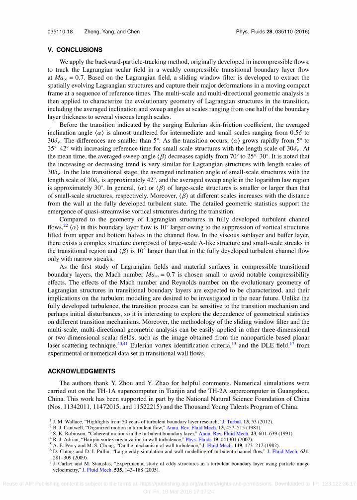
The temporal evolution of ⟨β⟩ for filtered component fields at different τ in the logarithmiclayer and ⟨β⟩ for the plane-cuts at different wall distances at τ = 2 are shown in Figs. 19(a) and19(b), respectively. The averaged sweep angle ⟨β⟩ in Fig. 19(a) is sketched by dashed lines inFigs. 17 and 18, which depict the decrease of ⟨β⟩ during the evolution for both scales. As shownin Fig. 18(a), the small-scale structures with large ⟨β⟩ appear at early times. After τ = 0.75, thesmall-scale structures are rapidly stretched along the streamwise direction in Figs. 18(c)–18(e).Based on Table III, we obtain the corresponding location xc(0.75) = 4.1 where the notable growth

Reuse of AIP Publishing content is subject to the terms at: https://publishing.aip.org/authors/rights-and-permissions. Downloaded to IP: 123.122.36.17

On: Fri, 18 Mar 2016 17:17:24

035110-16 Zheng, Yang, and Chen Phys. Fluids 28, 035110 (2016)

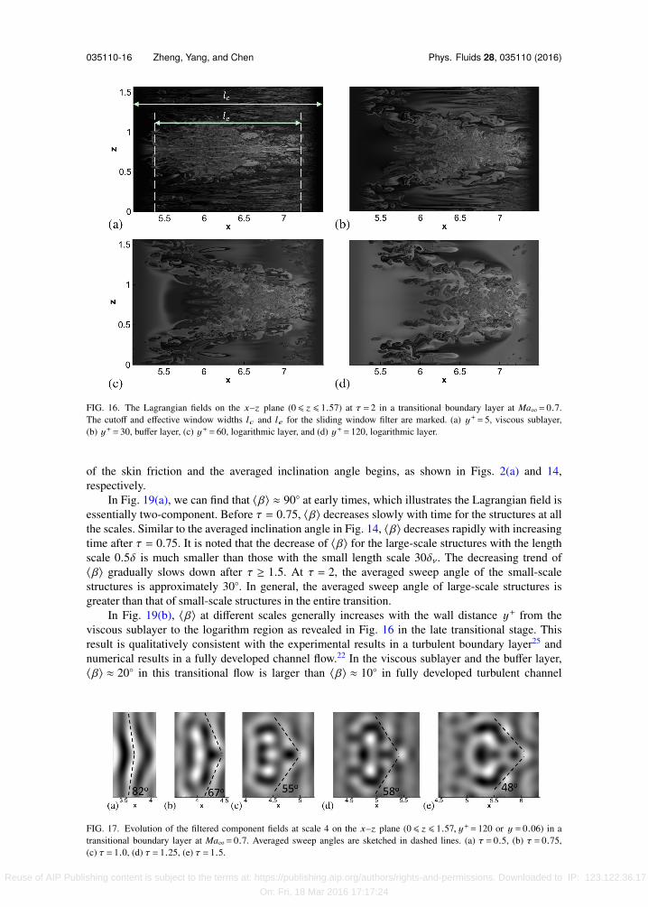
FIG. 16. The Lagrangian fields on the x–z plane (0 6 z 6 1.57) at τ = 2 in a transitional boundary layer at Ma∞= 0.7.The cutoff and effective window widths lc and le for the sliding window filter are marked. (a) y+= 5, viscous sublayer,(b) y+= 30, buffer layer, (c) y+= 60, logarithmic layer, and (d) y+= 120, logarithmic layer.

of the skin friction and the averaged inclination angle begins, as shown in Figs. 2(a) and 14,respectively.

In Fig. 19(a), we can find that ⟨β⟩ ≈ 90◦ at early times, which illustrates the Lagrangian field isessentially two-component. Before τ = 0.75, ⟨β⟩ decreases slowly with time for the structures at allthe scales. Similar to the averaged inclination angle in Fig. 14, ⟨β⟩ decreases rapidly with increasingtime after τ = 0.75. It is noted that the decrease of ⟨β⟩ for the large-scale structures with the lengthscale 0.5δ is much smaller than those with the small length scale 30δν. The decreasing trend of⟨β⟩ gradually slows down after τ ≥ 1.5. At τ = 2, the averaged sweep angle of the small-scalestructures is approximately 30◦. In general, the averaged sweep angle of large-scale structures isgreater than that of small-scale structures in the entire transition.

In Fig. 19(b), ⟨β⟩ at different scales generally increases with the wall distance y+ from theviscous sublayer to the logarithm region as revealed in Fig. 16 in the late transitional stage. Thisresult is qualitatively consistent with the experimental results in a turbulent boundary layer25 andnumerical results in a fully developed channel flow.22 In the viscous sublayer and the buffer layer,⟨β⟩ ≈ 20◦ in this transitional flow is larger than ⟨β⟩ ≈ 10◦ in fully developed turbulent channel

FIG. 17. Evolution of the filtered component fields at scale 4 on the x–z plane (0 6 z 6 1.57, y+= 120 or y = 0.06) in atransitional boundary layer at Ma∞= 0.7. Averaged sweep angles are sketched in dashed lines. (a) τ = 0.5, (b) τ = 0.75,(c) τ = 1.0, (d) τ = 1.25, (e) τ = 1.5.

Reuse of AIP Publishing content is subject to the terms at: https://publishing.aip.org/authors/rights-and-permissions. Downloaded to IP: 123.122.36.17

On: Fri, 18 Mar 2016 17:17:24

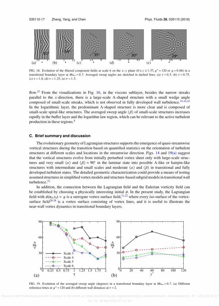
035110-17 Zheng, Yang, and Chen Phys. Fluids 28, 035110 (2016)

FIG. 18. Evolution of the filtered component fields at scale 6 on the x–z plane (0 6 z 6 1.57, y+= 120 or y = 0.06) in atransitional boundary layer at Ma∞= 0.7. Averaged sweep angles are sketched in dashed lines. (a) τ = 0.5, (b) τ = 0.75,(c) τ = 1.0, (d) τ = 1.25, (e) τ = 1.5.

flow.22 From the visualizations in Fig. 16, in the viscous sublayer, besides the narrow streaksparallel to the x-direction, there is a large-scale Λ-shaped structure with a small wedge anglecomposed of small-scale streaks, which is not observed in fully developed wall turbulence.15,16,22

In the logarithmic layer, the predominant Λ-shaped structure is more clear and is composed ofsmall-scale spiral-like structures. The averaged sweep angle ⟨β⟩ of small-scale structures increasesrapidly in the buffer layer and the logarithm law region, which can be relevant to the active turbulentproduction in these regions.4

C. Brief summary and discussion

The evolutionary geometry of Lagrangian structures supports the emergence of quasi-streamwisevortical structures during the transition based on quantified statistics on the orientation of turbulentstructures at different scales and locations in the streamwise direction. Figs. 14 and 19(a) suggestthat the vortical structures evolve from initially perturbed vortex sheet only with large-scale struc-tures and very small ⟨α⟩ and ⟨β⟩ ≈ 90◦ in the laminar state into possible Λ-like or hairpin-likestructures with intermediate and small scales and moderate ⟨α⟩ and ⟨β⟩ in transitional and fullydeveloped turbulent states. The detailed geometric characterization could provide a means of testingassumed structures in simplified vortex models and structure-based subgrid models in transitional wallturbulence.22

In addition, the connection between the Lagrangian field and the Eulerian vorticity field canbe established by choosing a physically interesting initial φ. In the present study, the Lagrangianfield with φ(x0, t0) = y is a surrogate vortex-surface field,21,22 where every iso-surface of the vortex-surface field20,38 is a vortex surface consisting of vortex lines, and it is useful to illustrate thenear-wall vortex dynamics in transitional boundary layers.

FIG. 19. Evolution of the averaged sweep angle (degrees) in a transitional boundary layer at Ma∞= 0.7. (a) Differentreference times at y+= 120 and (b) different wall distances at τ = 2.

Reuse of AIP Publishing content is subject to the terms at: https://publishing.aip.org/authors/rights-and-permissions. Downloaded to IP: 123.122.36.17

On: Fri, 18 Mar 2016 17:17:24

035110-18 Zheng, Yang, and Chen Phys. Fluids 28, 035110 (2016)

V. CONCLUSIONS

We apply the backward-particle-tracking method, originally developed in incompressible flows,to track the Lagrangian scalar field in a weakly compressible transitional boundary layer flowat Ma∞ = 0.7. Based on the Lagrangian field, a sliding window filter is developed to extract thespatially evolving Lagrangian structures and capture their major deformations in a moving compactframe at a sequence of reference times. The multi-scale and multi-directional geometric analysis isthen applied to characterize the evolutionary geometry of Lagrangian structures in the transition,including the averaged inclination and sweep angles at scales ranging from one half of the boundarylayer thickness to several viscous length scales.

Before the transition indicated by the surging Eulerian skin-friction coefficient, the averagedinclination angle ⟨α⟩ is almost unaltered for intermediate and small scales ranging from 0.5δ to30δν. The differences are smaller than 5◦. As the transition occurs, ⟨α⟩ grows rapidly from 5◦ to35◦–42◦ with increasing reference time for small-scale structures with the length scale of 30δν. Atthe mean time, the averaged sweep angle ⟨β⟩ decreases rapidly from 70◦ to 25◦–30◦. It is noted thatthe increasing or decreasing trend is very similar for Lagrangian structures with length scales of30δν. In the late transitional stage, the averaged inclination angle of small-scale structures with thelength scale of 30δν is approximately 42◦, and the averaged sweep angle in the logarithm law regionis approximately 30◦. In general, ⟨α⟩ or ⟨β⟩ of large-scale structures is smaller or larger than thatof small-scale structures, respectively. Moreover, ⟨β⟩ at different scales increases with the distancefrom the wall at the fully developed turbulent state. The detailed geometric statistics support theemergence of quasi-streamwise vortical structures during the transition.

Compared to the geometry of Lagrangian structures in fully developed turbulent channelflows,22 ⟨α⟩ in this boundary layer flow is 10◦ larger owing to the suppression of vortical structureslifted from upper and bottom halves in the channel flow. In the viscous sublayer and buffer layer,there exists a complex structure composed of large-scale Λ-like structure and small-scale streaks inthe transitional region and ⟨β⟩ is 10◦ larger than that in the fully developed turbulent channel flowonly with narrow streaks.

As the first study of Lagrangian fields and material surfaces in compressible transitionalboundary layers, the Mach number Ma∞ = 0.7 is chosen small to avoid notable compressibilityeffects. The effects of the Mach number and Reynolds number on the evolutionary geometry ofLagrangian structures in transitional boundary layers are expected to be characterized, and theirimplications on the turbulent modeling are desired to be investigated in the near future. Unlike thefully developed turbulence, the transition process can be sensitive to the transition mechanism andperhaps initial disturbances, so it is interesting to explore the dependence of geometrical statisticson different transition mechanisms. Moreover, the methodology of the sliding window filter and themulti-scale, multi-directional geometric analysis can be easily applied in other three-dimensionalor two-dimensional scalar fields, such as the image obtained from the nanoparticle-based planarlaser-scattering technique,40,41 Eulerian vortex identification criteria,13 and the DLE field,17 fromexperimental or numerical data set in transitional wall flows.

ACKNOWLEDGMENTS

The authors thank Y. Zhou and Y. Zhao for helpful comments. Numerical simulations werecarried out on the TH-1A supercomputer in Tianjin and the TH-2A supercomputer in Guangzhou,China. This work has been supported in part by the National Natural Science Foundation of China(Nos. 11342011, 11472015, and 11522215) and the Thousand Young Talents Program of China.

1 J. M. Wallace, “Highlights from 50 years of turbulent boundary layer research,” J. Turbul. 13, 53 (2012).2 B. J. Cantwell, “Organized motion in turbulent flow,” Annu. Rev. Fluid Mech. 13, 457–515 (1981).3 S. K. Robinson, “Coherent motions in the turbulent boundary layer,” Annu. Rev. Fluid Mech. 23, 601–639 (1991).4 R. J. Adrian, “Hairpin vortex organization in wall turbulence,” Phys. Fluids 19, 041301 (2007).5 A. E. Perry and M. S. Chong, “On the mechanism of wall turbulence,” J. Fluid Mech. 119, 173–217 (1982).6 D. Chung and D. I. Pullin, “Large-eddy simulation and wall modelling of turbulent channel flow,” J. Fluid Mech. 631,

281–309 (2009).7 J. Carlier and M. Stanislas, “Experimental study of eddy structures in a turbulent boundary layer using particle image

velocimetry,” J. Fluid Mech. 535, 143–188 (2005).

Reuse of AIP Publishing content is subject to the terms at: https://publishing.aip.org/authors/rights-and-permissions. Downloaded to IP: 123.122.36.17

On: Fri, 18 Mar 2016 17:17:24

035110-19 Zheng, Yang, and Chen Phys. Fluids 28, 035110 (2016)

8 B. Ganapathisubramani, E. K. Longmire, and I. Marusic, “Experimental investigation of vortex properties in a turbulentboundary layer,” Phys. Fluids 18, 055105 (2006).

9 P. R. Spalart, “Direct simulation of a turbulent boundary layer up to Rθ = 1410,” J. Fluid Mech. 187, 61–98 (1988).10 J. Jeong, F. Hussain, W. Schoppa, and J. Kim, “Coherent structures near the wall in a turbulent channel flow,” J. Fluid Mech.

332, 185–214 (1997).11 M. J. Ringuette, M. Wu, and M. P. Martin, “Coherent structures in direct numerical simulation of turbulent boundary layers

at Mach 3,” J. Fluid Mech. 594, 59–69 (2008).12 S. Pirozzoli, M. Bernardini, and F. Grasso, “Characterization of coherent vortical structures in a supersonic turbulent bound-

ary layer,” J. Fluid Mech. 613, 205–231 (2008).13 X. Wu and P. Moin, “Direct numerical simulation of turbulence in a nominally zero-pressure-gradient flat-plate boundary

layer,” J. Fluid Mech. 630, 5–41 (2009).14 Y.-B. Chu and X.-Y. Lu, “Topological evolution in compressible turbulent boundary layers,” J. Fluid Mech. 733, 414–438

(2013).15 S. J. Kline, W. C. Reynolds, F. A. Schraub, and P. W. Runstadler, “The structure of turbulent boundary layers,” J. Fluid

Mech. 30, 741–773 (1967).16 C. B. Lee and J. Z. Wu, “Transition in wall-bounded flows,” Appl. Mech. Rev. 61, 030802 (2008).17 M. A. Green, C. W. Rowley, and G. Haller, “Detection of Lagrangian coherent structures in three-dimensional turbulence,”

J. Fluid Mech. 572, 111–120 (2007).18 G. Haller, “Lagrangian coherent structures,” Annu. Rev. Fluid Mech. 47, 137–161 (2015).19 Y. Yang, D. I. Pullin, and I. Bermejo-Moreno, “Multi-scale geometric analysis of Lagrangian structures in isotropic turbu-

lence,” J. Fluid Mech. 654, 233–270 (2010).20 Y. Yang and D. I. Pullin, “On Lagrangian and vortex-surface fields for flows with Taylor–Green and Kida–Pelz initial

conditions,” J. Fluid Mech. 661, 446–481 (2010).21 Y. Zhao, Y. Yang, and S. Chen, “Evolution of material surfaces in the temporal transition in channel flow,” J. Fluid Mech.

(in press).22 Y. Yang and D. I. Pullin, “Geometric study of Lagrangian and Eulerian structures in turbulent channel flow,” J. Fluid Mech.

674, 67–92 (2011).23 T. Theodorsen, “Mechanism of turbulence,” in Proceedings of the Second Midwestern Conference on Fluid Mechanics

(Ohio State University, Columbus, OH, 1952).24 M. R. Head and P. Bandyopadhyay, “New aspects of turbulent boundary-layer structure,” J. Fluid Mech. 107, 297–338

(1981).25 L. Ong and J. M. Wallace, “Joint probability density analysis of the structure and dynamics of the vorticity field of a turbulent

boundary layer,” J. Fluid Mech. 367, 291–328 (1998).26 S. K. Robinson, “Space-time correlation measurements in a compressible turbulent boundary layer,” AIAA Paper No.

86-1130, 1986.27 N. Okamoto, K. Yoshimatsu, K. Schneider, M. Farge, and Y. Kaneda, “Coherent vortices in high resolution direct numerical

simulation of homogeneous isotropic turbulence: A wavelet viewpoint,” Phys. Fluids 19, 115109 (2007).28 T. Leung, N. Swaminathan, and P. A. Davidson, “Geometry and interaction of structures in homogeneous isotropic turbu-

lence,” J. Fluid Mech. 710, 453–481 (2012).29 E. Candes, L. Demanet, D. Donoho, and L. Ying, “Fast discrete curvelet transforms,” Multiscale Model. Simul. 5, 861–899

(2006).30 J. D. Anderson, Fundamentals of Aerodynamics, 4th ed. (McGraw-Hill, 2010).31 M. R. Malik, “Numerical methods for hypersonic boundary layer stability,” J. Comput. Phys. 86, 376–413 (1990).32 X. Li, D. Fu, and Y. Ma, “Direct numerical simulation of hypersonic boundary layer transition over a blunt cone with a

small angle of attack,” Phys. Fluids 22, 025105 (2010).33 Y. Zhou, X.-L. Li, D.-X. Fu, and Y.-W. Ma, “Coherent structures in transition of a flat-plate boundary layer at Ma = 0.7,”

Chin. Phys. Lett. 24, 147 (2007).34 F. Ducros, P. Comte, and M. Lesieur, “Large-eddy simulation of transition to turbulence in a boundary layer developing

spatially over a flat plate,” J. Fluid Mech. 326, 1–36 (1996).35 S. Pirozzoli, F. Grasso, and T. B. Gatski, “Direct numerical simulation and analysis of a spatially evolving supersonic

turbulent boundary layer at M = 2.25,” Phys. Fluids 16, 530 (2004).36 F. M. White, Viscous Fluid Flow, 3rd ed. (McGraw-Hill, 2006).37 S. B. Pope, Turbulent Flows (Cambridge University Press, 2000).38 Y. Yang and D. I. Pullin, “Evolution of vortex-surface fields in viscous Taylor–Green and Kida–Pelz flows,” J. Fluid Mech.

685, 146–164 (2011).39 L. Kleiser and T. A. Zang, “Numerical simulation of transition in wall-bounded shear flows,” Annu. Rev. Fluid Mech. 23,

495–537 (1991).40 Y. X. Zhao, S. H. Yi, L. F. Tian, and Z. Y. Cheng, “Supersonic flow imaging via nanoparticles,” Sci. China, Ser. E: Technol.

Sci. 52, 3640–3648 (2009).41 B. Wang, W. Liu, Y. Zhao, X. Fan, and C. Wang, “Experimental investigation of the micro-ramp based shock wave and

turbulent boundary layer interaction control,” Phys. Fluids 24, 055110 (2012).

Reuse of AIP Publishing content is subject to the terms at: https://publishing.aip.org/authors/rights-and-permissions. Downloaded to IP: 123.122.36.17

On: Fri, 18 Mar 2016 17:17:24