Evolution of the Theory of Mind - Becker Friedman Institute · Evolution of the Theory of Mind Daniel Monte, S~ao Paulo School of Economics (EESP-FGV) Nikolaus Robalino, Simon Fraser

Evolution of the Theory of Mind

Daniel Monte, Sao Paulo School of Economics (EESP-FGV)

Nikolaus Robalino, Simon Fraser University

Arthur Robson, Simon Fraser University

Conference “Biological Basis of Economic Preferences andBehavior”

Becker Friedman Institute, University of Chicago

May 5, 2012

0-0

0-1

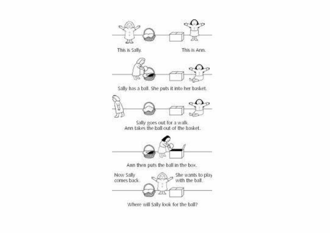
The “Theory of Mind” (TOM) refers to the ability to ascribeagency to other individuals (and to oneself), to ascribe beliefs anddesires, more particularly, to one and all. This ability is manifestin non-autistic humans beyond infancy, but less obvious in otherspecies. A key early experiment is the Sally-Ann test. (Baron-Cohen, Leslie, Frith (1985), for example.)

0-2

0-3

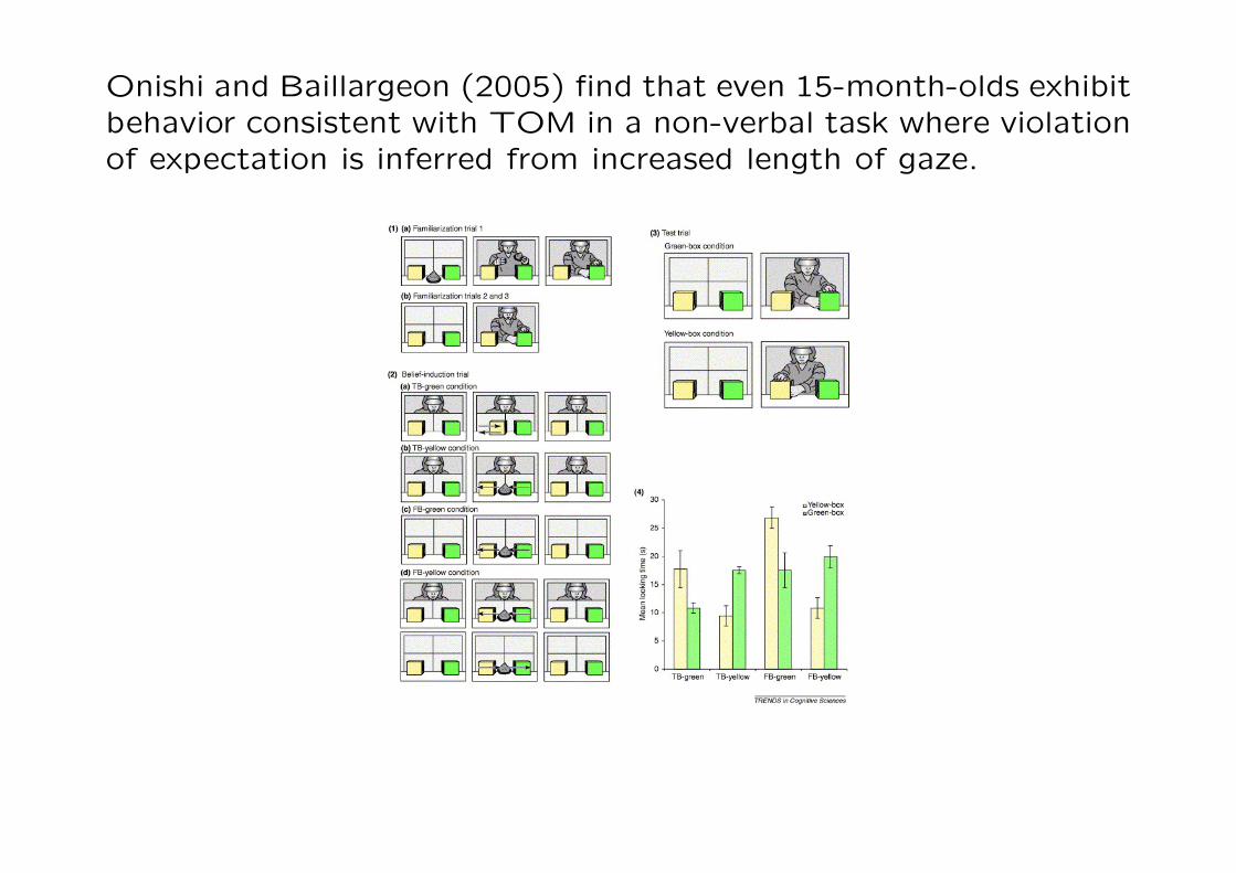
Onishi and Baillargeon (2005) find that even 15-month-olds exhibitbehavior consistent with TOM in a non-verbal task where violationof expectation is inferred from increased length of gaze.

0-4

Onishi and Baillargeon (2005) find that even 15-month-olds exhibitbehavior consistent with TOM in a non-verbal task where violationof expectation is inferred from increased length of gaze.

Would this work on nonhuman species too?

0-5

Brodmann area 10

0-6

Such an ability is crucial to game theory. That is, it is usuallynecessary to understand an opponent’s payoffs, to put oneself inhis shoes, that is, in order to predict his behavior and therefore tochoose an optimal strategy oneself.

0-7

Such an ability is crucial to game theory. That is, it is usuallynecessary to understand an opponent’s payoffs, to put oneself inhis shoes, that is, in order to predict his behavior and therefore tochoose an optimal strategy oneself.

0-8

This ability might be seen as an aspect of Machiavellian Intelli-gence. The hypothesis here is that our intelligence evolved underpressure to outsmart our conspecifics. (See, for example, Byrneand Whiten (1998).) This is often contrasted with the EcologicalIntelligence Hypothesis—that the nonhuman environment providedthe impetus (Robson and Kaplan AER (2003), for example).

0-9

This ability might be seen as an aspect of Machiavellian Intelli-gence. The hypothesis here is that our intelligence evolved underpressure to outsmart our conspecifics. (See, for example, Byrneand Whiten (1998).) This is often contrasted with the EcologicalIntelligence Hypothesis—that the nonhuman environment providedthe impetus (Robson and Kaplan AER (2003), for example).

0-10

The present approach substantially extends and generalizes Rob-son ”Why Would Nature Give Individuals Utility Functions?” JPE(2001), who considered the evolutionary rationale for own utility ina decision-theoretic framework. In contrast, we consider a rationalefor knowing the utility functions of others in a strategic framework.In both cases, however, it is the need to address novelty that isthe evolutionary impetus.

0-11

The present approach substantially extends and generalizes Rob-son ”Why Would Nature Give Individuals Utility Functions?” JPE(2001), who considered the evolutionary rationale for own utility ina decision-theoretic framework. In contrast, we consider a rationalefor knowing the utility functions of others in a strategic framework.In both cases, however, it is the need to address novelty that isthe evolutionary impetus.

The approach here contrasts with that of a small literature rep-resented by Stahl GEB (1993), who considers the evolutionaryadvantage of greater strategic sophistication. (See also Crawfordand Iriberri (2007) and Mohlin (2012), for example.) Stahl arguesthat it may be better to be (lucky and) dumb than to be smart. Weobtain a clearer advantage to smart mainly because we consider agame with outcomes that are randomly selected from a growingoutcome set, rather than a particular fixed game.

0-12

Here we investigate the evolutionary basis of an ability to acquirethe preferences of an opponent. We contrast such more sophis-ticated agents with naive agents who adapt to each game as inevolutionary game theory and as in “reinforcement learning” inpsychology.

0-13

Consider an anecdote about vervet monkeys from Cheney and Sey-farth (1990). When a male vervet sought to join Kitui’s group,where Kitui was bottom-ranked, Kitui might make the leopardwarning cry. The interloper would stay in his tree, his plans thwarted.The TOM Kitui understood the effect of such a cry on the othersand was deliberately deceptive. A naive Kitui, in contrast, hadno model of other vervets’ preferences and beliefs. Inadvertently,perhaps, he once made the leopard warning in such a circumstanceand it worked. (That the latter option was actually true was sug-gested by Kitui occasionally walking on the ground towards theother male, alarm calling all the while.)

0-14

Consider an anecdote about vervet monkeys from Cheney and Sey-farth (1990). When a male vervet sought to join Kitui’s group,where Kitui was bottom-ranked, Kitui might make the leopardwarning cry. The interloper would stay in his tree, his plans thwarted.The TOM Kitui understood the effect of such a cry on the othersand was deliberately deceptive. A naive Kitui, in contrast, hadno model of other vervets’ preferences and beliefs. Inadvertently,perhaps, he once made the leopard warning in such a circumstanceand it worked. (That the latter option was actually true was sug-gested by Kitui occasionally walking on the ground towards theother male, alarm calling all the while.)

0-15

Here we model the contest between TOMer’s and naive players.We consider games of perfect information, the simplest of whichhas two stages. If player 1 is naive, she must see all games beforelearning to play appropriately; if she is a TOMer, she must merelysee player 2 confronted with all possible pairs of outcomes. Theedge for the TOMer’s then derives from there being many moregames than pairs of outcomes.

0-16

Here we model the contest between TOMer’s and naive players.We consider games of perfect information, the simplest of whichhas two stages. If player 1 is naive, she must see all games beforelearning to play appropriately; if she is a TOMer, she must merelysee player 2 confronted with all possible pairs of outcomes. Theedge for the TOMer’s then derives from there being many moregames than pairs of outcomes.

We demonstrate this edge by considering an environment that be-comes richer as time passes. If the environment rapidly becomesmore complex, neither type is able to keep up; if the environmentonly slowly becomes more complex both types can keep up. In anintermediate range, however, the TOMers learn essentially every-thing, the naive types essentially nothing.

0-17

0-18

Two-Stage Model

Two “large” populations—“player 1’s” (“she’s”) and “player 2’s”(“he’s”). At t = 1, 2, ..., randomly paired to play a simple two-stagegame of perfect information. Game tree with exactly two movesat each of the non-terminal nodes. The games vary on account ofthe outcomes assigned to the terminal nodes. Each player has afixed strict preference ordering over the countably infinite set X.

P1

L

~~|||||||| R

BBB

BBBB

B

P2

L

~~}}}}}}}

R��

P2

L��

R

AAA

AAAA

x1 x2 x3 x4

0-19

Two-Stage Model

Two “large” populations—“player 1’s” (“she’s”) and “player 2’s”(“he’s”). At t = 1, 2, ..., randomly paired to play a simple two-stagegame of perfect information. Game tree with exactly two movesat each of the non-terminal nodes. The games vary on account ofthe outcomes assigned to the terminal nodes. Each player has afixed strict preference ordering over the countably infinite set X.

P1

L

~~|||||||| R

BBB

BBBB

B

P2

L

~~}}}}}}}

R��

P2

L��

R

AAA

AAAA

x1 x2 x3 x4

0-20

The two-stage game at t is Γt. At each t Γt is completed by arandom draw of four outcomes from the finite Xt ⊂ X. If anytwo of the outcomes are identical, it is known to the sophisticatedplayers that they are indifferent; if the outcomes are different, theyinduce a strict preference ordering for the player in question, butthis strict preference is not known to other players.

0-21

The two-stage game at t is Γt. At each t Γt is completed by arandom draw of four outcomes from the finite Xt ⊂ X. If anytwo of the outcomes are identical, it is known to the sophisticatedplayers that they are indifferent; if the outcomes are different, theyinduce a strict preference ordering for the player in question, butthis strict preference is not known to other players.

Naive players adapt to each game; theory-of-mind (TOM) playersconstruct the opponent’s preferences.

0-22

Each history of outcomes and choices is public information. If amixed strategy is used, this would be observed, although just onthe nodes that are reached. We consider only symmetric strategies.

0-23


There are no feedback effects of individuals’ actions on their op-ponents and so there is no incentive to play non-myopically. Player2’s have no interest in player 1’s payoffs. Further, the player 1’sreact only to the distribution of player 2 choices. Since any partic-ular player 2 has no effect on this distribution of player 2 choices,any particular player 2 is myopic.

0-24


There are no feedback effects of individuals’ actions on their op-ponents and so there is no incentive to play non-myopically. Player2’s have no interest in player 1’s payoffs. Further, the player 1’sreact only to the distribution of player 2 choices. Since any partic-ular player 2 has no effect on this distribution of player 2 choices,any particular player 2 is myopic.

The outcome sets increase over time, capturing growing complex-ity. There is a sequence t1, ..., tk, ..., where tk is the arrival date ofthe k-th new object. The initial set of objects is X0 with size n.Thus, in tk to tk+1 − 1 the number of objects is n+ k. We assumetk = bkαc, for α ≥ 0.

0-25

0-26

A naive player adapts to each game Γt. For simplicity, we assumethat if the game Γt is novel, the naive player plays inappropriatelyat t, say by randomizing 50-50 at each decision node. However, thenext time this same game in encountered, the naive player makesthe appropriate choices. That is, the adaptive learning here is asfast as it possibly could be. Even with this advantage, however,the naive types will be outdone by the TOM types.

0-27

A naive player adapts to each game Γt. For simplicity, we assumethat if the game Γt is novel, the naive player plays inappropriatelyat t, say by randomizing 50-50 at each decision node. However, thenext time this same game in encountered, the naive player makesthe appropriate choices. That is, the adaptive learning here is asfast as it possibly could be. Even with this advantage, however,the naive types will be outdone by the TOM types.

In contrast, a player has a theory of mind if she knows that heropponent will take binary decisions that are consistent with someinitially unknown preference ordering. She does not avail herself ofthe transitivity of her opponent’s preferences. Our comparison ofthe naive type with the TOM is then a comparison of the speedof the associated learning processes.

0-28

We now characterize the maximum amount of knowledge in thisenvironment for naive and TOM players. For naive player 1’s or 2’sat date t the maximum amount of knowledge is simply the numberof games, Gt, say. We have that

Gt = |Xt|4

0-29

We now characterize the maximum amount of knowledge in thisenvironment for naive and TOM players. For naive player 1’s or 2’sat date t the maximum amount of knowledge is simply the numberof games, Gt, say. We have that

Gt = |Xt|4

If the number of distinct games that have played before date t isKNt , then we consider the fraction of these that are known to any

naive player as

LNt =KNt

Gt.

0-30

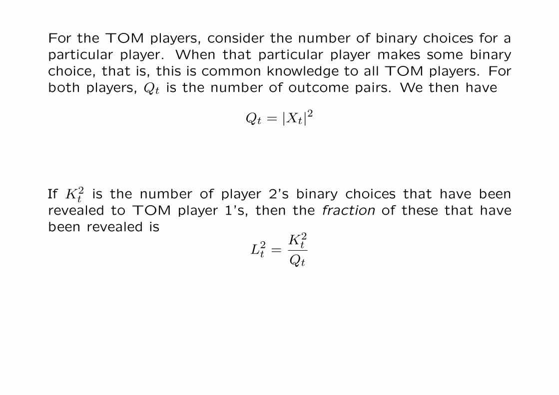
For the TOM players, consider the number of binary choices for aparticular player. When that particular player makes some binarychoice, that is, this is common knowledge to all TOM players. Forboth players, Qt is the number of outcome pairs. We then have

Qt = |Xt|2

0-31

For the TOM players, consider the number of binary choices for aparticular player. When that particular player makes some binarychoice, that is, this is common knowledge to all TOM players. Forboth players, Qt is the number of outcome pairs. We then have

Qt = |Xt|2

If K2t is the number of player 2’s binary choices that have been

revealed to TOM player 1’s, then the fraction of these that havebeen revealed is

L2t =

K2t

Qt

0-32

We now have the main result for the two-stage game case—

Theorem 1 All the results here concern player 1—

i) If α ∈ [0, 2) then L2t → 0 and LNt → 0 as t→∞ in probability. That

is, both the sophisticated and the naive type are overwhelmed bythe rapid rate of arrival of new outcomes.

ii) If α ∈ (4,∞), then L2t → 1 and LNt → 1 as t → ∞ in probability.

That is, the rate of arrival of new outcomes is slow enough thatboth types are able to essentially learn everything.

iii) Finally, however, if α ∈ (2, 4), then L2t → 1 but LNt → 0 as t→∞

in probability. That is, for this intermediate range of arrival rates,the TOM type learns essentially everything, while the naive typelearns essentially nothing.

0-33

Except possibly for the values 2 and 4, the results are dramatic—either everything is learnt in the limit or nothing is. Indeed, therange where nothing is learnt is inescapable in that the arrival rateof novelty outstrips there the maximum rate at which learning canoccur. So the real contribution is to show the less obvious resultthat full learning occurs essentially whenever it is even possible thatit could.

0-34

Except possibly for the values 2 and 4, the results are dramatic—either everything is learnt in the limit or nothing is. Indeed, therange where nothing is learnt is inescapable in that the arrival rateof novelty outstrips there the maximum rate at which learning canoccur. So the real contribution is to show the less obvious resultthat full learning occurs essentially whenever it is even possible thatit could.

In terms of the contest between the two types, the existence of aninterval over which the TOM type learns everything and the naivetype learns nothing implies we can finesse the issue of consideringpayoffs explicitly. Whatever these payoffs might be it is clear thatthe TOM type is outdoing the naive type in this intermediate range.

0-35

Revealed Preference

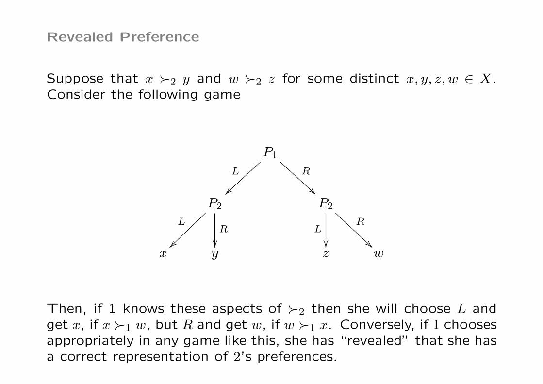
Suppose that x �2 y and w �2 z for some distinct x, y, z,w ∈ X.Consider the following game

P1

L

~~|||||||| R

BBB

BBBB

B

P2

L

~~~~~~~~~~

R

��

P2

L

��

R

AAA

AAAA

A

x y z w

0-36

Revealed Preference

Suppose that x �2 y and w �2 z for some distinct x, y, z,w ∈ X.Consider the following game

P1

L

~~|||||||| R

BBB

BBBB

B

P2

L

~~~~~~~~~~

R

��

P2

L

��

R

AAA

AAAA

A

x y z w

Then, if 1 knows these aspects of �2 then she will choose L andget x, if x �1 w, but R and get w, if w �1 x. Conversely, if 1 choosesappropriately in any game like this, she has “revealed” that she hasa correct representation of 2’s preferences.

0-37

There is no simpler way to ensure that player 1 always choosescorrectly in all two-stage games, for all preferences �1.

0-38

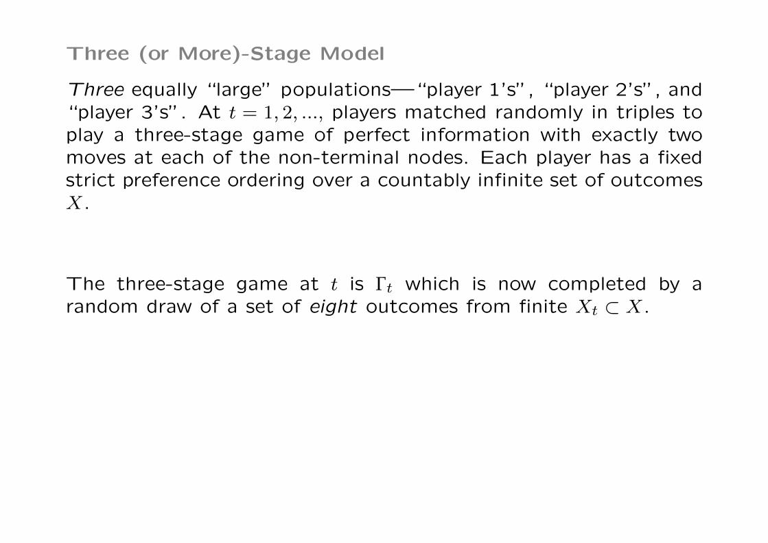
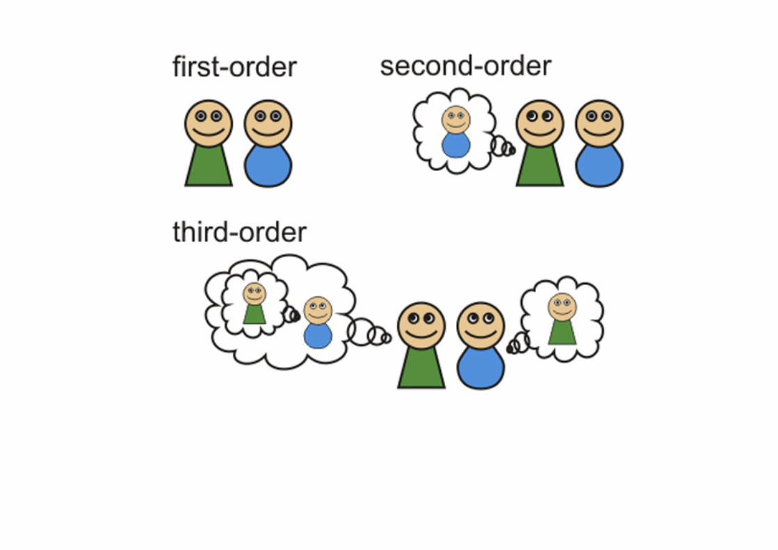
Three (or More)-Stage Model

Three equally “large” populations—“player 1’s”, “player 2’s”, and“player 3’s”. At t = 1, 2, ..., players matched randomly in triples toplay a three-stage game of perfect information with exactly twomoves at each of the non-terminal nodes. Each player has a fixedstrict preference ordering over a countably infinite set of outcomesX.

0-39



The three-stage game at t is Γt which is now completed by arandom draw of a set of eight outcomes from finite Xt ⊂ X.

0-40



The three-stage game at t is Γt which is now completed by arandom draw of a set of eight outcomes from finite Xt ⊂ X.

0-41

P1

L

~~|||||||| R

$$III

IIII

II

P2

L

~~|||||||| R

BBB

BBBB

B P2 · · ·P3

P3

L

~~}}}}}}}

R��

P3

L

~~}}}}}}}}

R��

x1 x2 x3 x4

0-42

P1

L

~~|||||||| R

$$III

IIII

II

P2

L

~~|||||||| R

BBB

BBBB

B P2 · · ·P3

P3

L

~~}}}}}}}

R��

P3

L

~~}}}}}}}}

R��

x1 x2 x3 x4

What if the naive type of player 2, for example, were less naive,keying not on the entire three stage-game, but on the subgamederiving from each choice by player 1? A somewhat weaker versionof the argument goes through.

0-43

The type of the last player, now player 3, is again irrelevant, sinceplayer 3 uses only his own preferences. TOM player 2’s constructa simple model of player 3’s preferences. TOM player 1’s con-struct simple models of the other two players’ preferences, and theplayer 1’s also need to know that the player 2’s know player 3’spreferences.

0-44

0-45

Individual players again have no incentive to mislead the opponentabout one’s preferences. In the three-stage case, this observationhas force only for the player 2’s and 3’s. That is, the player 1’scannot advantageously mislead the player 2’s or 3’s because theplayer 2’s and 3’s do not consider 1’s preferences. The player1’s and 2’s react only to the distribution of choices made by theplayer 3’s. Since any particular player 3 then has no effect on thedistribution of player 3 choices, and hence cannot affect the playof the player 1’s or 2’s, any such particular player 3 must behavemyopically. Similarly, the player 1’s only react to the distribution ofchoices made by the player 2’s and so there is no incentive for theplayer 2’s to distort the choices made in order to influence player1’s.

0-46

Individual players again have no incentive to mislead the opponentabout one’s preferences. In the three-stage case, this observationhas force only for the player 2’s and 3’s. That is, the player 1’scannot advantageously mislead the player 2’s or 3’s because theplayer 2’s and 3’s do not consider 1’s preferences. The player1’s and 2’s react only to the distribution of choices made by theplayer 3’s. Since any particular player 3 then has no effect on thedistribution of player 3 choices, and hence cannot affect the playof the player 1’s or 2’s, any such particular player 3 must behavemyopically. Similarly, the player 1’s only react to the distribution ofchoices made by the player 2’s and so there is no incentive for theplayer 2’s to distort the choices made in order to influence player1’s.

We again focus on outcome sets that increase over time, describedprecisely as before.

0-47

As before, a player who is naive adapts to each game Γt as a distinctcircumstance, but takes only two trials to play appropriately.

0-48


Again, in contrast, a player with a theory of mind knows her oppo-nent will take decisions that are consistent with some preferenceordering. She has the capacity to learn this ordering.

0-49


Again, in contrast, a player with a theory of mind knows her oppo-nent will take decisions that are consistent with some preferenceordering. She has the capacity to learn this ordering.

0-50

For naive player 1’s, 2’s or 3’s at date t the maximum amount ofknowledge is again the number of games, Gt, say. Now

Gt = |Xt|8

0-51

For naive player 1’s, 2’s or 3’s at date t the maximum amount ofknowledge is again the number of games, Gt, say. Now

Gt = |Xt|8

If the number of distinct games that have played before at date tis KN

t , the fraction of games that are known to any naive player is

LNt =KNt

Gt.

0-52

For the players with a theory of mind, it is convenient to considerthe number of binary choices that can be made by a particularplayer, j, say. When player j makes some binary choice, that is,this is common knowledge to all TOM players. For all players, thenumber of outcome pairs is as before—

Qt = |Xt|2.

If Kjt is the number of player j = 2, 3 ’s binary choices that have

been revealed to all TOM players, as common knowledge, then thefraction of these is

Ljt =Kjt

Qt.

0-53

The following is then the main result for the three-stage gamecase. We first show that player 2 derives an advantage from TOMover naivete, essentially as in the two-stage game. Once player 2is of TOM type, we then show that player 1 derives an advantagefrom TOM over naivete.

Theorem 2 A) Suppose that player 1 plays in an arbitrary fashion.Then we have the following results for player 2—

i) If α ∈ [0, 2) then L3t → 0 and LNt → 0 as t → ∞ in probability.

That is, both the sophisticated and the naive type of player 2 areoverwhelmed by the rapid rate of arrival of new outcomes.

ii) If α ∈ (8,∞), then L3t → 1 and LNt → 1 as t → ∞ in probability.

That is, the rate of arrival of new outcomes is slow enough thatboth types are able to essentially learn everything.

iii) Finally, however, if α ∈ (2, 8), then L3t → 1 but LNt → 0 as t→∞

in probability. That is, for this intermediate range of arrival rates,the TOM type learns essentially everything, while the naive typelearns essentially nothing.

0-54

B) Suppose that player 2 is TOM. Then we have the followingresults for player 1—

i) If α ∈ [0, 2) then L2t → 0, L3

t → 0, and LNt → 0, as t → ∞ inprobability. That is, both the sophisticated and the naive type areoverwhelmed by the rapid rate of arrival of new outcomes.

ii) If α ∈ (8,∞), then L2t → 1, L3

t → 1, and LNt → 1 as t → ∞ inprobability. That is, the rate of arrival of new outcomes is slowenough that both types are able to essentially learn everything.

iii) Finally, however, if α ∈ (2, 8), then L2t → 1, L3

t → 1, but LNt → 0as t → ∞ in probability. That is, for this intermediate range ofarrival rates, the TOM type learns essentially everything, while thenaive type learns essentially nothing.

0-55

Again, the results are dramatic—except possibly at two points, ei-ther everything is learnt in the limit or nothing is. Again, whennothing is learnt, it is because it is simply mechanically impossibleto keep up with the rate of novelty, so that the key contribution ofthis theorem is to show that everything is learnt essentially when-ever this is not mechanically ruled out.

0-56

Again, the results are dramatic—except possibly at two points, ei-ther everything is learnt in the limit or nothing is. Again, whennothing is learnt, it is because it is simply mechanically impossibleto keep up with the rate of novelty, so that the key contribution ofthis theorem is to show that everything is learnt essentially when-ever this is not mechanically ruled out.

As in the two-stage case, there is then an interval over which theTOM type learns everything and the naive type learns nothing.This interval is larger in the three-stage game case because thenaive types of player 1 or 2 face a larger set of possible games,now with eight outcomes drawn from the outcome set, and hencecan only keep up with a slower rate of novelty. On the other hand,for the result in A), the TOM type of player 2 still needs to knowonly how player 3 would make each possible binary choice.

0-57

For B), the situation for player 1 is more complex, because player 1not only needs to know both player 2’s preferences and player 3’s,but also needs to know that player 2 knows player 3’s preferences.This would seem likely to shift the transition point from no learn-ing to full learning for TOM player 1’s. However, the followingobservations apply. As long as α > 2, player 1 will learn player 3’spreferences completely in the limit. In addition, at the same timethat 3’s choices reveal information about 3’s preferences to player1, they reveal the same information to player 2 and player 1 knowsthis. But now, given only that α > 2, player 1 can also completelylearn player 2’s preferences.

0-58

For B), the situation for player 1 is more complex, because player 1not only needs to know both player 2’s preferences and player 3’s,but also needs to know that player 2 knows player 3’s preferences.This would seem likely to shift the transition point from no learn-ing to full learning for TOM player 1’s. However, the followingobservations apply. As long as α > 2, player 1 will learn player 3’spreferences completely in the limit. In addition, at the same timethat 3’s choices reveal information about 3’s preferences to player1, they reveal the same information to player 2 and player 1 knowsthis. But now, given only that α > 2, player 1 can also completelylearn player 2’s preferences.

For A), the large numbers of player 1’s, 2’s and 3’s ensure thatthe player 2’s should be sequentially rational. It might somehowbe to the player 2s’ overall advantage to be perceived by the player1’s as naive rather than sophisticated. However, when there aremany player 2’s, with some of these naive and some sophisticated,each individual player 2 has no effect on player 1’s perceptions ofthe distribution of player 2’s. Thus each sophisticated sequentiallyrational player 2 outperforms each naive player 2.

0-59

It is always clear that learning must be slow if L2t is close to one.

When α > 2, however, the proof involves showing this is the onlycircumstance under which learning is slow. There are two com-plicating factors. The first is that there are subgames in which2’s choice cannot reveal information about 2’s preferences becausethere is insufficient knowledge about 3’s preferences and thereforechoices.

0-60

It is always clear that learning must be slow if L2t is close to one.

When α > 2, however, the proof involves showing this is the onlycircumstance under which learning is slow. There are two com-plicating factors. The first is that there are subgames in which2’s choice cannot reveal information about 2’s preferences becausethere is insufficient knowledge about 3’s preferences and thereforechoices.

The second factor concerns the existence of player 2 subgames withoutcomes that are avoided by player 3, thus making it difficult toreveal information about 2’s preferences. Such games arise evenas t −→∞. However, A1 implies that these problematic games area vanishing fraction of all games as t −→∞.

0-61

These results extend straightforwardly to a perfect informationgame with S stages and S players. When considering the sophis-tication of player s we assume that players s+ 1, ...,S are alreadyTOM. The critical value of α for any TOM player remains 2, for alls. The critical value of α for a naive player grows with the numberof possible games that can be formed.

0-62

Further Extensions

How much do the current results depend on the particular modeldescribed here? Although the environment is rather particular, it isbest seen merely as a test to discriminate between the underlyingcharacteristics of ToM’s and of the naive players.

0-63

Further Extensions

How much do the current results depend on the particular modeldescribed here? Although the environment is rather particular, it isbest seen merely as a test to discriminate between the underlyingcharacteristics of ToM’s and of the naive players.

What about games with imperfect information? With multipleNash equilibria, it is not clear how to disentangle the lack of knowl-edge of payoffs from the lack of information about which equilib-rium is to be played, at least in the absence of strong assumptions.Perhaps normal form games crop up along with the games of per-fect information emphasized here, using outcomes drawn from thesame set. Whether or not any learning can be accomplished onsuch normal form games, our approach shows that learning wouldarise based only on the games of perfect information.

0-64

Within the class of games of perfect information, it is only forsimplicity that we restrict attention to a fixed game tree. Thetree itself could be random: it might involve a random number ofmoves or a random order of play, for example. Similarly, playerscould be allowed to move multiple times, and so on.

0-65

Within the class of games of perfect information, it is only forsimplicity that we restrict attention to a fixed game tree. Thetree itself could be random: it might involve a random number ofmoves or a random order of play, for example. Similarly, playerscould be allowed to move multiple times, and so on.

Similarly, the assumption that individuals have a strict ranking overeach distinct pair of outcomes is basically innocuous. If indifferenceis allowed, suppose, for example, that individuals randomize overeach pair of indifferent outcomes. The indifference of player ibetween z and z′ would then be common knowledge to the ToMtypes, if ever player i chose z over z′ and z′ over z.

0-66

We assume here that ToM types do not apply transitivity in theirdeductions about the preferences of other players. This mightmake a difference to the relevant ranges of the growth parameterα. The new value of α cannot exceed 2, since applying transitivitycould not be disadvantageous. It could not lower the critical valueof α below 1.

0-67

We assume here that ToM types do not apply transitivity in theirdeductions about the preferences of other players. This mightmake a difference to the relevant ranges of the growth parameterα. The new value of α cannot exceed 2, since applying transitivitycould not be disadvantageous. It could not lower the critical valueof α below 1.

More sophisticated naive types could clearly do better than theones we describe here. If naive types assign beliefs to subgames,rather than to entire games, for example, they would do as wellas ToM types in the two stage game case. More generally, withthree or more stages, such more sophisticated naive players woulddo better than the naive players considered here, but not as wellas the sophisticated players.

0-68

Experiments

It would be interest to experimentally implement the model, per-haps simplified to have no innovation. Also it seems we might notneed a very large number of subjects in each of the I pools. Inducethe same preferences over a large set of outcomes for each of theplayer i’s for i = 1, ..., I by using monetary payoffs. No player knowsthe other players’ payoffs. Play the game otherwise as above. Howfast would players learn other players’ preferences? Would they becloser to the sophisticated ToM types described above or to thenaive types? How would the number of stages I affect matters?

0-69

The End

0-70

Sketch of Proofs

We treat a general case with I stages and A choices at each decisionnode.

0-71

Sketch of Proofs


No learning in the limit

If outcomes arrive at too fast a rate, it is straightforward to provethat learning cannot occur even when the greatest possible amountof information is revealed in every period.

0-72

Sketch of Proofs




Lemma 1 In each of the following convergence is sure.

i) Suppose α ∈ [0, 2). Then Lti −→ 0 for each preference type i =1, ..., I.

ii) Suppose there are T terminal nodes. If α ∈ [0,T ), then LNt −→ 0.

0-73

Sketch of Proofs




Lemma 1 In each of the following convergence is sure.

i) Suppose α ∈ [0, 2). Then Lti −→ 0 for each preference type i =1, ..., I.

ii) Suppose there are T terminal nodes. If α ∈ [0,T ), then LNt −→ 0.

0-74

Results About Learning

Theorem 1 is a special case of Theorem 2. Attention is restrictedto the ToM players, and so to the Lit’s. (The corresponding claimabout the naive types goes through with minor changes to theanalysis.) As hypothesized in Theorem 2, when considering Lit,players i+ 1, ..., , I are taken to be ToM.

0-75

Results About Learning

Theorem 1 is a special case of Theorem 2. Attention is restrictedto the ToM players, and so to the Lit’s. (The corresponding claimabout the naive types goes through with minor changes to theanalysis.) As hypothesized in Theorem 2, when considering Lit,players i+ 1, ..., , I are taken to be ToM.

Auxiliary Results

The first minor result, Proposition 1, relates how much is com-monly known about i’s preferences over pairs of outcomes to whatis commonly known about i’s preferences over A-tuples of out-comes. The need for this result can be finessed, for expositionalsimplicity, by setting A = 2.

0-76

The gist of Proposition 2 is the following. Suppose types i, ..., Iare all ToM and that Li+1

t , ...,LIt each converge to one in probabil-ity. Then, in the limit, the probability of revealing new informationabout i’s preferences is small only if the fraction of extant knowl-edge about preferences, Lit, is close to one. Indeed, although theprobability of revealing new information about i is clearly small if1−Lit is small, the converse is not obviously true.

0-77

The gist of Proposition 2 is the following. Suppose types i, ..., Iare all ToM and that Li+1

t , ...,LIt each converge to one in probabil-ity. Then, in the limit, the probability of revealing new informationabout i’s preferences is small only if the fraction of extant knowl-edge about preferences, Lit, is close to one. Indeed, although theprobability of revealing new information about i is clearly small if1−Lit is small, the converse is not obviously true.

Proposition 2, however, establishes an appropriate lower bound.This bound decomposes the expected amount learnt into a factorinvolving of 1− Lit, reflecting what is yet to be revealed about i’spreferences, and a residual term.

0-78

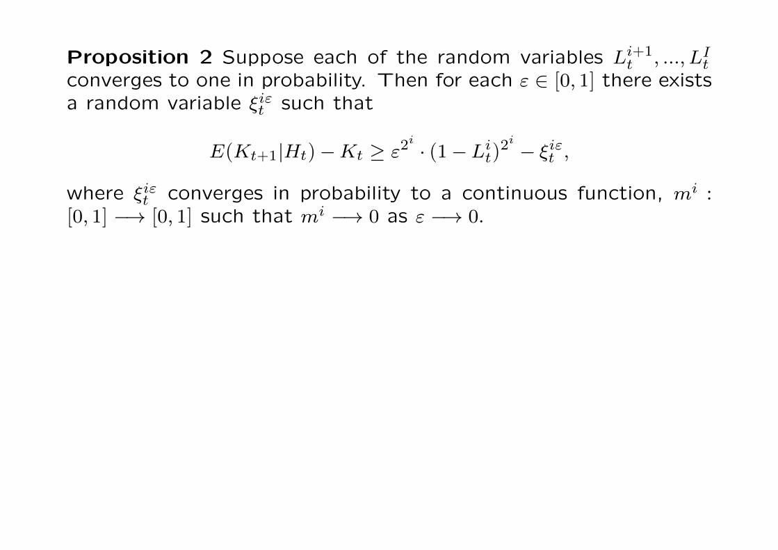
Proposition 2 Suppose each of the random variables Li+1t , ...,LIt

converges to one in probability. Then for each ε ∈ [0, 1] there existsa random variable ξiεt such that

E(Kt+1|Ht)−Kt ≥ ε2i· (1−Lit)2

i− ξiεt ,

where ξiεt converges in probability to a continuous function, mi :[0, 1] −→ [0, 1] such that mi −→ 0 as ε −→ 0.

0-79

Proposition 2 Suppose each of the random variables Li+1t , ...,LIt

converges to one in probability. Then for each ε ∈ [0, 1] there existsa random variable ξiεt such that


i− ξiεt ,

where ξiεt converges in probability to a continuous function, mi :[0, 1] −→ [0, 1] such that mi −→ 0 as ε −→ 0.

Proposition 2 is the heart of the matter. Consider the case of playerI. What is a lower bound on the probability that something newwill be learned about this player’s preferences? Such a lower boundarises from the event that every pair of outcomes that followschoice by player I is unfamiliar to the ToM players. This lowerbound is then [1−LIt ]2

I−1 ≥ [1−LIt ]2I.

0-80

For players who are not last, the situation is more complex. Thereare two complicating factors. The first is that there are i-typesubgames in which i’s choice cannot reveal information about i’spreferences because there is insufficient knowledge about the re-maining players’ choices.

0-81


The second factor concerns the existence of i-type subgames withoutcomes that are avoided by the remaining opponents, thus mak-ing it difficult to reveal information about i’s preferences. Suchgames arise even as t −→∞. However, A1 implies that these prob-lematic games are a vanishing fraction of all games as t −→ ∞.

0-82


The second factor concerns the existence of i-type subgames withoutcomes that are avoided by the remaining opponents, thus mak-ing it difficult to reveal information about i’s preferences. Suchgames arise even as t −→∞. However, A1 implies that these prob-lematic games are a vanishing fraction of all games as t −→ ∞.

These two complicating factors account for the additional multi-plicative and additive terms in the bound obtained in Proposition2.

0-83

Proposition 3 then essentially completes the proof of Theorem 2(and Theorem 1) by applying the result of Proposition 2.

0-84

Proposition 3 then essentially completes the proof of Theorem 2(and Theorem 1) by applying the result of Proposition 2.

Proposition 3. Suppose that, for each ε ∈ [0, 1] there exists arandom variable ξiεt such that


i− ξiεt ,

where ξiεt converges in probability to a continuous function, mi :[0, 1] −→ [0, 1] such that mi −→ 0 as ε −→ 0. If, in addition, α > 2,then Lit converges to one in probability.

0-85

Consider the case that I = 3 for simplicity of exposition and con-sider player 2. Assume for the moment that L2

t converges in proba-bility to the random variable L. Fix η > 0 and let A denote the eventL < 1− η. Given the above facts about the probability of new infor-mation being revealed, the random variable E(K2

t+τ |ht) is boundedbelow asymptotically by K2

t + η2 · τ , on A, as τ →∞., That is, on A,in the limit learning occurs at least linearly in τ . Observe now thatQt+τ is of order τ2/α. Then, dividing through by the non-randomQt+τ , we obtain that E(L2

t |ht)→∞ on A. Since by definition L2t is

bounded above by one surely, it must be that P (A) = 0. That is, ifα > 2, and L2

t converges in probability to L, it must be that L = 1almost surely.

0-86

It remains then to show the convergence in probability just as-sumed. We do this by showing that the Lt processes lie in a classof generalized martingales. Consider the following—

0-87


Weak-Submartingale in the Limit: The adapted process (Lt,ht) is aweak sub-martingale in the limit (w-submil) if, for each η > 0, thereis a T such that τ ≥ t ≥ T implies P (E(Lτ |ht)−Lt ≥ −η) > 1− η, a.e.and uniformly in τ .

0-88


Weak-Submartingale in the Limit: The adapted process (Lt,ht) is aweak sub-martingale in the limit (w-submil) if, for each η > 0, thereis a T such that τ ≥ t ≥ T implies P (E(Lτ |ht)−Lt ≥ −η) > 1− η, a.e.and uniformly in τ .

Egghe (1984) shows that bounded weak sub-martingales in thelimit have limits in probability.

0-89

Given the above, we need to prove that the Lt sequences are w-submils. Clearly the Lt process has the sub-martingale property inbetween arrival dates. However, at an arrival date, Lt is discountedby the factor Qt

Qt+1, and increases by at most 1

Qt+1. The key is then

to show that the sequence of Lt at the arrival dates is neverthelessa w-submil. This follows because there is a process converging to1 such that Lt at the arrival dates can only decrease if it is greaterthan this process or close to it.

0-90

The End

0-91

Documents

Evolution of the Theory of Mind - Becker Friedman Institute · Evolution of the Theory of Mind Daniel Monte, S~ao Paulo School of Economics (EESP-FGV) Nikolaus Robalino, Simon Fraser