Evolution of the martensitic transformation in shape memoryalloys under high strain rates

D. Saletti1,a, S. Pattofatto1, and H. Zhao1

Laboratoire de Mecanique et Technologie (LMT-Cachan), ENS-Cachan/CNRS-UMR8535/UniversiteParis 6, 61 avenue du President Wilson, F-94235 Cachan Cedex, France

Abstract. The specific properties of the shape memory alloys are mainly due to themartensitic transformation occuring in the material when mechanical or thermal load-ings are applied. Here, the effect of strain rate on the transformation on an NiTi SMA isstudied in tension. Different tests were performed at different strain rates in the range of0,0001 /s to 15 /s. Two distinct methods were used to measure the extension rate of themartensitic phase region in the specimen: digital image correlation technique and infraredthermography (IR during quasi-static tensile tests only). For the dynamic tensile tests,a Split Hopkinson Tensile Bar set-up was used with a fast camera recording at 45’000fps. A superimposition of DIC and IR measurements in time and space can be done dur-ing quasi-static tests and results show that the temperature peak, as expected, follows thetransformation front. As a consequence of the former validation of the DIC procedure,the velocity of the transformation front at high strain rate is deduced from space-time fig-ures. As a conclusion, in the range of strain rates investigated in this paper, no strain ratesensitivity is observed for dynamics of extension of the transformation region.

1 Introduction

Due to two of their specific properties, namely superelasticity and the shape memory effect, shapememory alloys (SMA) have a great potential of applications in a lot of innovative technologies. Inparticular, the NiTi-based SMA are widely used as biomaterials (to manufacture stents for heart arteryfor instance) or in mechanical applications such as in the automotive industry, household appliances,and many other everyday goods.

In such SMA, two phases can be found, separately or combined. The transformation from a phaseto the other is triggered when the material is undergoing variation of temperature or mechanical sol-licitation, or both. By analogy with steel, the transformation, the mother phase and the daughter phaseare respectively called martensitic transformation, austenite phase and martensite phase. In the caseof SMA, martensitic transformation is reversible. Superelastic properties of the SMA are shown on astress-strain curve, which is decomposed in three parts: first the elastic response of the material in a fullaustenite phase, then generally a plateau where martensitic transformation is occuring and propagat-ing, which is visible through imaging techniques ([1]), and finally the homogeneous elastic responseof the material in a full-martensitic phase. Studies have already been done on the influence of strainrate on the macroscopic behaviour of the SMA ([2]). The higher the strain rate, the more the slope ofthe plateau part of the stress-strain curve raises. This can be found in compression as well as in tension,despite the asymmetry between the two modes of loading. Assumptions have been made to explain thechange in high strain rate response ([3]) and refer to the adiabatic regime at the transformation front,preventing the austenite phase from tranforming unless the level of stress is raised.

a e-mail: saletti@lmt.ens-cachan.fr

© Owned by the authors, published by EDP Sciences, 2010DOI:10.1051/epjconf/20100629008EPJ Web of Conferences 6, 29008 (2010) 6

This is an Open Access article distributed under the terms of the Creative Commons Attribution-Noncommercial License 3.0, which permits unrestricted use, distribution, and reproduction in any noncommercial medium, provided the original work is properly cited.

Article disponible sur le site http://www.epj-conferences.org ou http://dx.doi.org/10.1051/epjconf/20100629008

EPJ Web of Conferences

In this paper the effect of strain rate on the martensitic transformation in tension on a NiTi SMAis studied. Different tests were performed at different strain rates in the range of 10−4 s−1 to 15 s−1,extending the range of observations of the investigations previously done by [4]. Methods were usedto measure the velocity of the propagation of the martensitic phase in the specimen: digital imagecorrelation (DIC) techniques and infrared thermography (IR, during the quasi-static tensile tests only).

2 Experimental techniques

The measurement techniques employed in this study were different depending on the strain rate ap-plied. For the 1.67 · 10−4 s−1 strain rate, a classical electromechanical INSTRON machine was usedassociated with a reflex camera recording at 0.25 frame per second (fps) and an IR thermography de-vice. For the 1.67 · 10−2 s−1 strain rate, the same machine was used but with a fast camera recordingat 125 fps. For the 16 s−1 strain rate which corresponds to the dynamic tensile test, a Split HopkinsonTensile Bar (SHTB) set-up was used with a fast camera recording at 45’000 fps.

2.1 Specimen characteristics

A single NiTi plate-shape specimen was used for the whole of the experiments. The dimensions are60 × 3 × 1.2 mm3. Tensile tests were performed at three different strain rate ranges and at room tem-perature, clearly above the characteristic A f temperature so that for stress-free condition the specimenis in a full austenite state. For all the experiments, the specimen is fixed between two tabs that canfurther be screwed (i) in the bars for dynamic tensile experiment, (ii) in a clamping system for staticexperiments. This allows to be more confident in the comparison of experimental results obtained withdifferent devices.

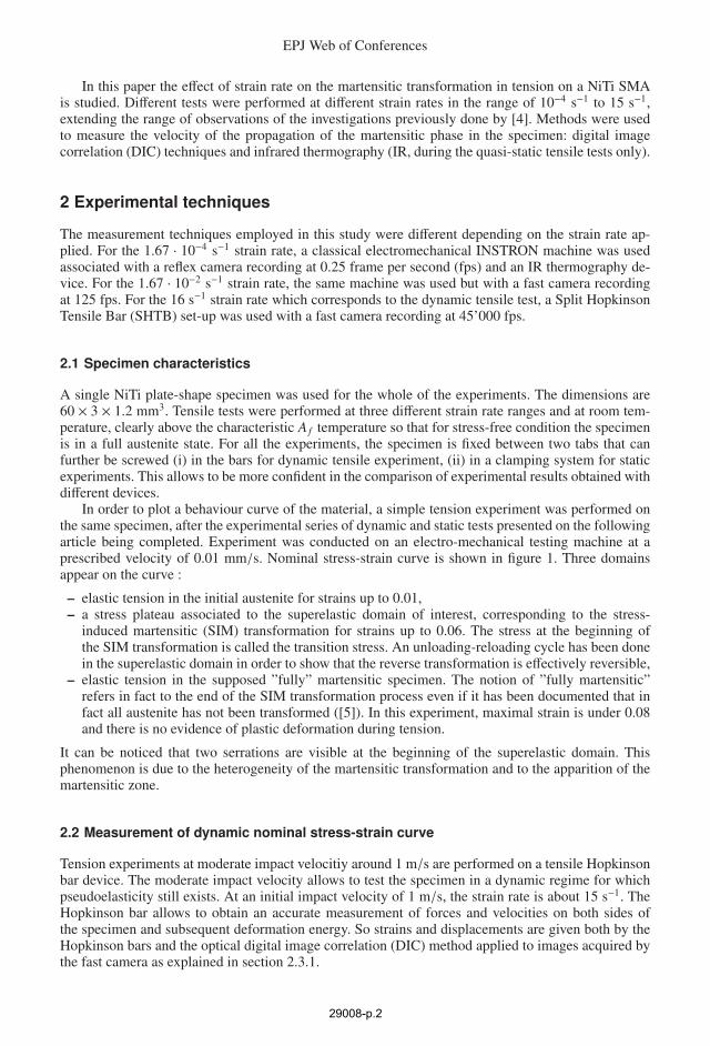
In order to plot a behaviour curve of the material, a simple tension experiment was performed onthe same specimen, after the experimental series of dynamic and static tests presented on the followingarticle being completed. Experiment was conducted on an electro-mechanical testing machine at aprescribed velocity of 0.01 mm/s. Nominal stress-strain curve is shown in figure 1. Three domainsappear on the curve :

– elastic tension in the initial austenite for strains up to 0.01,– a stress plateau associated to the superelastic domain of interest, corresponding to the stress-

induced martensitic (SIM) transformation for strains up to 0.06. The stress at the beginning ofthe SIM transformation is called the transition stress. An unloading-reloading cycle has been donein the superelastic domain in order to show that the reverse transformation is effectively reversible,

– elastic tension in the supposed ”fully” martensitic specimen. The notion of ”fully martensitic”refers in fact to the end of the SIM transformation process even if it has been documented that infact all austenite has not been transformed ([5]). In this experiment, maximal strain is under 0.08and there is no evidence of plastic deformation during tension.

It can be noticed that two serrations are visible at the beginning of the superelastic domain. Thisphenomenon is due to the heterogeneity of the martensitic transformation and to the apparition of themartensitic zone.

2.2 Measurement of dynamic nominal stress-strain curve

Tension experiments at moderate impact velocitiy around 1 m/s are performed on a tensile Hopkinsonbar device. The moderate impact velocity allows to test the specimen in a dynamic regime for whichpseudoelasticity still exists. At an initial impact velocity of 1 m/s, the strain rate is about 15 s−1. TheHopkinson bar allows to obtain an accurate measurement of forces and velocities on both sides ofthe specimen and subsequent deformation energy. So strains and displacements are given both by theHopkinson bars and the optical digital image correlation (DIC) method applied to images acquired bythe fast camera as explained in section 2.3.1.

29008-p.2

14th International Conference on Experimental Mechanics

A → SIM

A

SIM

serrations

0 0.02 0.04 0.06 0.080

50

100

150

200

250

300

350

Nominal Strain

Nom

inal

Str

ess

(MPa

)

Fig. 1. Static strain-stress curve at nominal strain rate of 1.67 · 10−4 s−1 at room temperature.

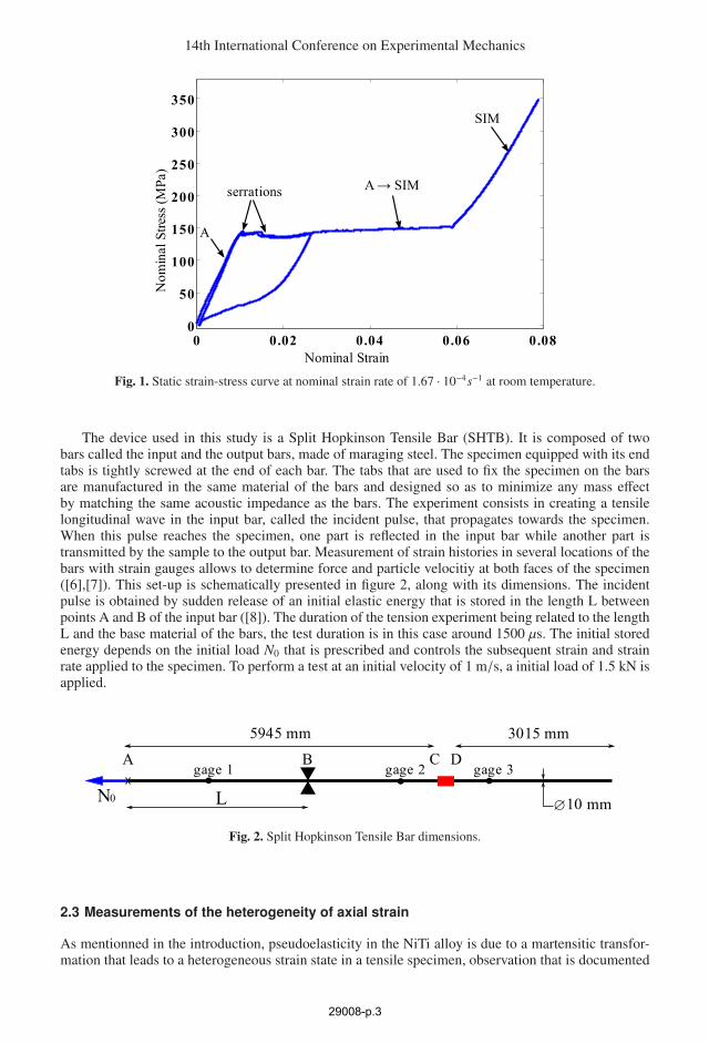
The device used in this study is a Split Hopkinson Tensile Bar (SHTB). It is composed of twobars called the input and the output bars, made of maraging steel. The specimen equipped with its endtabs is tightly screwed at the end of each bar. The tabs that are used to fix the specimen on the barsare manufactured in the same material of the bars and designed so as to minimize any mass effectby matching the same acoustic impedance as the bars. The experiment consists in creating a tensilelongitudinal wave in the input bar, called the incident pulse, that propagates towards the specimen.When this pulse reaches the specimen, one part is reflected in the input bar while another part istransmitted by the sample to the output bar. Measurement of strain histories in several locations of thebars with strain gauges allows to determine force and particle velocitiy at both faces of the specimen([6],[7]). This set-up is schematically presented in figure 2, along with its dimensions. The incidentpulse is obtained by sudden release of an initial elastic energy that is stored in the length L betweenpoints A and B of the input bar ([8]). The duration of the tension experiment being related to the lengthL and the base material of the bars, the test duration is in this case around 1500 µs. The initial storedenergy depends on the initial load N0 that is prescribed and controls the subsequent strain and strainrate applied to the specimen. To perform a test at an initial velocity of 1 m/s, a initial load of 1.5 kN isapplied.

A B C Dgage 1 gage 2 gage 3

L

5945 mm 3015 mm

N0 10 mm∅

Fig. 2. Split Hopkinson Tensile Bar dimensions.

2.3 Measurements of the heterogeneity of axial strain

As mentionned in the introduction, pseudoelasticity in the NiTi alloy is due to a martensitic transfor-mation that leads to a heterogeneous strain state in a tensile specimen, observation that is documented

29008-p.3

EPJ Web of Conferences

for static loadings. In order to follow this phenomenon at a tension velocity of 1 m/s, complementarymeasurements are conducted. Displacement and subsequent axial strain path along the specimen arecalculated by digital image correlation (DIC). Moreover, since martensitic transformation is exother-mic, infrared thermography (IRT) measurements are also a good mean to measure indirectly the loca-tion of the ongoing transformation. Optical and thermal measurements are obtained simultaneously onthe same thin specimen, on two opposite sides that are supposed to have the same thermo-mechanicalresponse. These two optical techniques are described in following sections, along with the experimen-tal strategy that has been implemented.

2.3.1 Digital Image Correlation (DIC) setup

For dynamic experiments, a fast camera (Photron) is used to acquire images at a frame rate of 45’000fps with a resolution of 896 × 64 pixels, an integration time of 12 µs and a spatial resolution of0.09 mm/pixel. For quasi-static tensile test, a reflex camera (Canon EOS) is used. The capture fre-quency is 0.25 fps (one image every four seconds) in a full resolution of 2314 × 3474 pixels, that givesa spatial resolution of 0.026 mm/pixel. In order to allow DIC computations, a speckle was applied onthe observed surface of the specimen with black and white paint. Moreover, to avoid heating of thespecimen surface, the lighting was realized with LED lights during the quasi-static experiments andwith short light exposition of the specimen during the dynamic experiments.

The principle of the DIC computation program (CorreliQ4) that was used is given as follows([9],elnasri07). Basically, pictures of the deforming specimen are taken during the experiments. Theprinciple is to relate two images f (x) and g(x) corresponding to two different steps of loading, througha displacement field u to be calculated. Considering the conservation of the brightness, the followingequation can be written, relating the image of reference f (x) and the deformed image g(x) through theunknown displacement u:

g(x) = f [x + u(x)] (1)Under the assumption that the image of reference is differentiable, the expression is developed in

Taylor series, and the displacement field u comes as the result of the minimization of the followingquadratic error:

η2 =

"[u(x) · ∇ f (x) + f (x) − g(x)]2 dx (2)

The last point of the specific Q4-method ([9]) is that the unknow displacement is decomposed overa set of scalar shape functions ψn(x) as follows:

u(x) =∑α,n

aαnψn(x)eα (3)

This leads to a linear system of equations that can be solved numerically through a spatial dis-cretization in elements of any domain of interest selected in the image of reference. It has been docu-mented that the performance of such a method is influenced by the size of the elements. Large size forthe elements tends to improve the accuracy of the computed displacement field but to the detrimentof spatial resolution. Then in the case of heterogeneous deformation, and in particular for localizeddeformation, the element size has to be a compromise between accuracy and spatial detection of thelocalized phenomenon. An element size around 30 × 30 pixels was found to be a good candidate inorder to observe the transforming zone while limiting noise effects in the computations.

During dynamic tensile tests, the specimen exhibited large displacements. In this case, a strategyof update was used: the image of reference is regularly updated and the calculation of displacementfield is performed by increments.

2.3.2 Infrared Thermography (IRT) setup

IRT pictures were acquired using an infrared camera (Jade CEDIP) with a resolution of 320× 240 pixels.For every test, the frame period is 25 fps, the integration time to acquire a picture is 310 µs and thespatial resolution is 0.27 mm/pixel.

29008-p.4

14th International Conference on Experimental Mechanics

All the experiments were performed at a room temperature (around 300 K). A thin layer of carbonblack powder was deposited on the surface in order to make its emissivity higher and more homoge-neous. Moreover, in order to improve the signal to noise ratio, and in particular to prevent effects ofperturbative reflections, the optical path between the lens and the surface of the specimen was shelteredby a ”tunnel cover” which inner surface was covered with black paint.

For the quasi-static tests, IRT measurements are given in addition to DIC measurements and usedas a validation of the DIC technique for the measurement of transforming regions in the specimen.IRT thermography was not tried during dynamic tensile tests and this will be part of a further study.

3 Analysis of the propagation velocity of the martensitic transformation onthe quasi-static cases

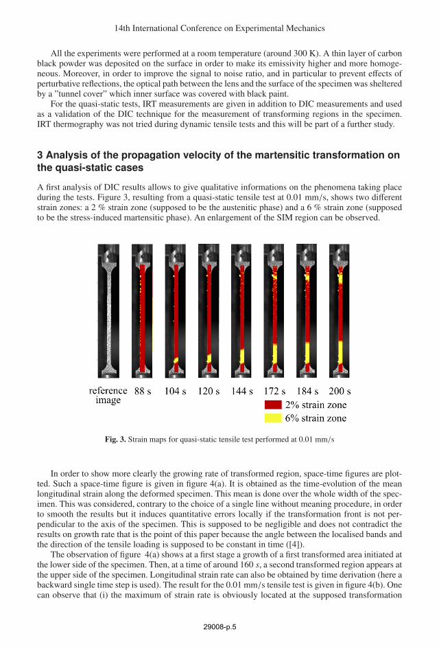
A first analysis of DIC results allows to give qualitative informations on the phenomena taking placeduring the tests. Figure 3, resulting from a quasi-static tensile test at 0.01 mm/s, shows two differentstrain zones: a 2 % strain zone (supposed to be the austenitic phase) and a 6 % strain zone (supposedto be the stress-induced martensitic phase). An enlargement of the SIM region can be observed.

Fig. 3. Strain maps for quasi-static tensile test performed at 0.01 mm/s

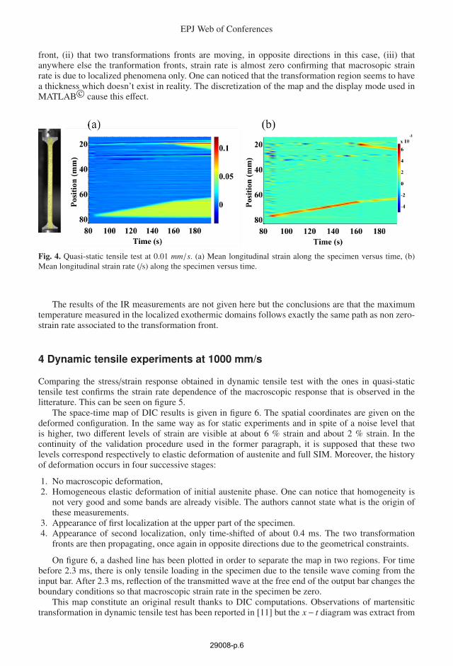
In order to show more clearly the growing rate of transformed region, space-time figures are plot-ted. Such a space-time figure is given in figure 4(a). It is obtained as the time-evolution of the meanlongitudinal strain along the deformed specimen. This mean is done over the whole width of the spec-imen. This was considered, contrary to the choice of a single line without meaning procedure, in orderto smooth the results but it induces quantitative errors locally if the transformation front is not per-pendicular to the axis of the specimen. This is supposed to be negligible and does not contradict theresults on growth rate that is the point of this paper because the angle between the localised bands andthe direction of the tensile loading is supposed to be constant in time ([4]).

The observation of figure 4(a) shows at a first stage a growth of a first transformed area initiated atthe lower side of the specimen. Then, at a time of around 160 s, a second transformed region appears atthe upper side of the specimen. Longitudinal strain rate can also be obtained by time derivation (here abackward single time step is used). The result for the 0.01 mm/s tensile test is given in figure 4(b). Onecan observe that (i) the maximum of strain rate is obviously located at the supposed transformation

29008-p.5

EPJ Web of Conferences

front, (ii) that two transformations fronts are moving, in opposite directions in this case, (iii) thatanywhere else the tranformation fronts, strain rate is almost zero confirming that macrosopic strainrate is due to localized phenomena only. One can noticed that the transformation region seems to havea thickness which doesn’t exist in reality. The discretization of the map and the display mode used inMATLAB c© cause this effect.

Fig. 4. Quasi-static tensile test at 0.01 mm/s. (a) Mean longitudinal strain along the specimen versus time, (b)Mean longitudinal strain rate (/s) along the specimen versus time.

The results of the IR measurements are not given here but the conclusions are that the maximumtemperature measured in the localized exothermic domains follows exactly the same path as non zero-strain rate associated to the transformation front.

4 Dynamic tensile experiments at 1000 mm/s

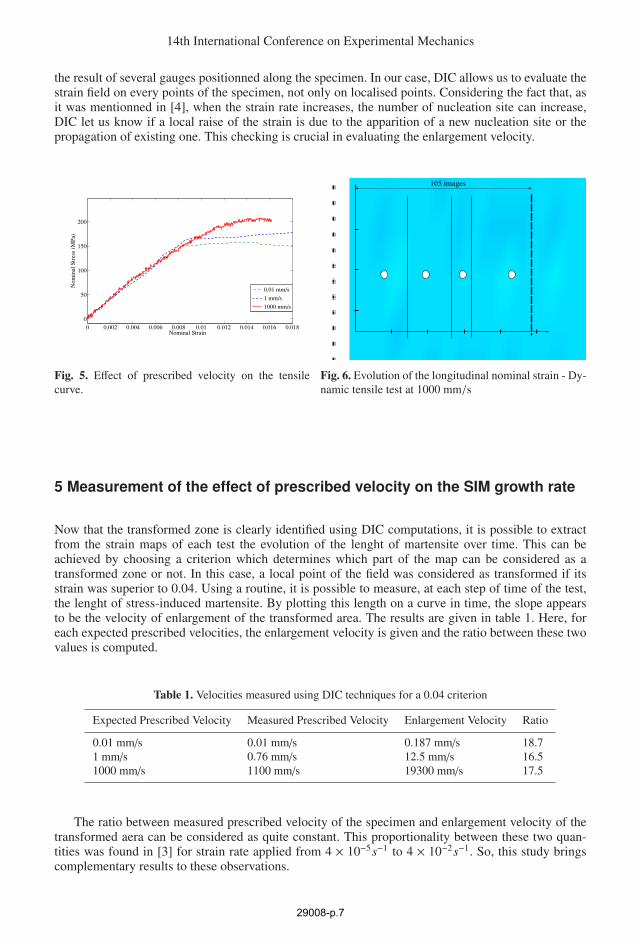
Comparing the stress/strain response obtained in dynamic tensile test with the ones in quasi-statictensile test confirms the strain rate dependence of the macroscopic response that is observed in thelitterature. This can be seen on figure 5.

The space-time map of DIC results is given in figure 6. The spatial coordinates are given on thedeformed configuration. In the same way as for static experiments and in spite of a noise level thatis higher, two different levels of strain are visible at about 6 % strain and about 2 % strain. In thecontinuity of the validation procedure used in the former paragraph, it is supposed that these twolevels correspond respectively to elastic deformation of austenite and full SIM. Moreover, the historyof deformation occurs in four successive stages:

1. No macroscopic deformation,2. Homogeneous elastic deformation of initial austenite phase. One can notice that homogeneity is

not very good and some bands are already visible. The authors cannot state what is the origin ofthese measurements.

3. Appearance of first localization at the upper part of the specimen.4. Appearance of second localization, only time-shifted of about 0.4 ms. The two transformation

fronts are then propagating, once again in opposite directions due to the geometrical constraints.

On figure 6, a dashed line has been plotted in order to separate the map in two regions. For timebefore 2.3 ms, there is only tensile loading in the specimen due to the tensile wave coming from theinput bar. After 2.3 ms, reflection of the transmitted wave at the free end of the output bar changes theboundary conditions so that macroscopic strain rate in the specimen be zero.

This map constitute an original result thanks to DIC computations. Observations of martensitictransformation in dynamic tensile test has been reported in [11] but the x− t diagram was extract from

29008-p.6

14th International Conference on Experimental Mechanics

the result of several gauges positionned along the specimen. In our case, DIC allows us to evaluate thestrain field on every points of the specimen, not only on localised points. Considering the fact that, asit was mentionned in [4], when the strain rate increases, the number of nucleation site can increase,DIC let us know if a local raise of the strain is due to the apparition of a new nucleation site or thepropagation of existing one. This checking is crucial in evaluating the enlargement velocity.

0 0.002 0.004 0.006 0.008 0.01 0.012 0.014 0.016 0.0180

50

100

150

200

Nominal Strain

Nom

inal

Str

ess

(MPa

)

0.01 mm/s

1 mm/s

1000 mm/s

Fig. 5. Effect of prescribed velocity on the tensilecurve.

105 images

31 2 4

Fig. 6. Evolution of the longitudinal nominal strain - Dy-namic tensile test at 1000 mm/s

5 Measurement of the effect of prescribed velocity on the SIM growth rate

Now that the transformed zone is clearly identified using DIC computations, it is possible to extractfrom the strain maps of each test the evolution of the lenght of martensite over time. This can beachieved by choosing a criterion which determines which part of the map can be considered as atransformed zone or not. In this case, a local point of the field was considered as transformed if itsstrain was superior to 0.04. Using a routine, it is possible to measure, at each step of time of the test,the lenght of stress-induced martensite. By plotting this length on a curve in time, the slope appearsto be the velocity of enlargement of the transformed area. The results are given in table 1. Here, foreach expected prescribed velocities, the enlargement velocity is given and the ratio between these twovalues is computed.

Table 1. Velocities measured using DIC techniques for a 0.04 criterion

Expected Prescribed Velocity Measured Prescribed Velocity Enlargement Velocity Ratio

0.01 mm/s 0.01 mm/s 0.187 mm/s 18.71 mm/s 0.76 mm/s 12.5 mm/s 16.51000 mm/s 1100 mm/s 19300 mm/s 17.5

The ratio between measured prescribed velocity of the specimen and enlargement velocity of thetransformed aera can be considered as quite constant. This proportionality between these two quan-tities was found in [3] for strain rate applied from 4 × 10−5s−1 to 4 × 10−2s−1. So, this study bringscomplementary results to these observations.

29008-p.7

EPJ Web of Conferences

6 Results and conclusion

Specific measurement techniques have been implemented in order to analyze the influence of nomi-nal strain rate on the growth rate of the SIM region in a NiTi specimen. Hopkinson bar measurementtechnique, DIC applied to quasi-static and dynamic experiment, and IR thermography for static exper-iments give accurate and relevant results. After synchronizing DIC and IR measurements in time andspace, a superimposition can be done and results show that the temperature peak, as expected, followsthe transformation front. Finally, the velocity of the propagation front is measured and we show thatit depends linearly on the prescribed velocity. As a conclusion, in the range of strain rates investigatedin this paper, no strain rate sensitivity is observed.

References

1. E.A. Pieczyska, S.P. Gadaj, W.K. Nowacki, H. Tobushi, Exp. Mech. 46,(2006) 531–542.2. S. Nemat-Nasser, J.Y. Choi, Acta Materialia 53,(2005) 449–454.3. J.A. Shaw, S. Kyriakides, J. Mech. Phys. Solids, 43,(1995) No.8 1243–1281.4. J.A. Shaw, S. Kyriakides, Acta Mater., 45,(1997) No.2 683–700.5. Brinson, Schmidt, Lammering, J. Mech. Phys. Solids, 52, (2004) 1549–1571.6. E.D.H. Davies, S.C. Hunter, J. Mech. Phys. Solids,11, (1963) 55–179.7. H. Zhao, G. Gary, J. Mech. Phys. Solids,45, (1997) No.7 1185–1202.8. G.H. Staab, A. Gilat, Exp. Mech., 31, (1991) No.3 232–235.9. G. Besnard, F. Hild, S. Roux, Exp. Mech., 46, (2006) No.6 789–804.10. I. Elnasri, S. Pattofatto, H. Zhao, H. Tsitsiris, F. Hild, Y. Girard, J. Mech. Phys. Solids, 55 (2007)

2652–2671.11. J. Niemczura, K. Ravi-Chandar, J. Mech. Phys. Solids, 54 (2006) 2136–2161.

29008-p.8