Embed Size (px)
Citation preview
Evolution of P2P Content Evolution of P2P Content DistributionDistribution
Pei CaoPei Cao

OutlineOutline
• History of P2P Content Distribution History of P2P Content Distribution ArchitecturesArchitectures
• Techniques to Improve GnutellaTechniques to Improve Gnutella
• Brief Overview of DHTBrief Overview of DHT
• Techniques to Improve BitTorrentTechniques to Improve BitTorrent
History of P2PHistory of P2P
• NapsterNapster
• GnutellaGnutella
• KaZaaKaZaa
• Distributed Hash TablesDistributed Hash Tables
• BitTorrentBitTorrent
NapsterNapster
• Centralized directoryCentralized directory– A central website to hold directory of A central website to hold directory of
contents of all peerscontents of all peers– Queries performed at the central Queries performed at the central
directorydirectory– File transfer occurs between peersFile transfer occurs between peers– Support arbitrary queriesSupport arbitrary queries– Con: Single point of failureCon: Single point of failure
GnutellaGnutella
• Decentralized homogenous peersDecentralized homogenous peers– No central directoryNo central directory– Queries performed distributed on peers Queries performed distributed on peers
via “flooding”via “flooding”– Support arbitrary queriesSupport arbitrary queries– Very resilient against failureVery resilient against failure– Problem: Doesn’t scaleProblem: Doesn’t scale
FastTrack/KaZaaFastTrack/KaZaa
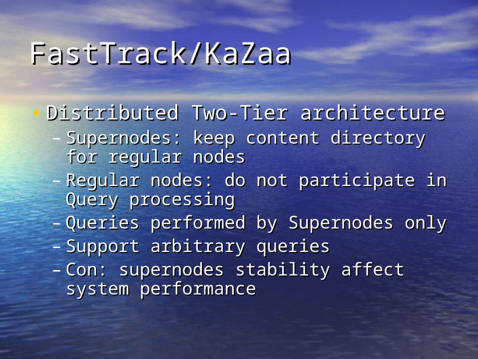
• Distributed Two-Tier architectureDistributed Two-Tier architecture– Supernodes: keep content directory for Supernodes: keep content directory for
regular nodesregular nodes– Regular nodes: do not participate in Regular nodes: do not participate in
Query processingQuery processing– Queries performed by Supernodes onlyQueries performed by Supernodes only– Support arbitrary queriesSupport arbitrary queries– Con: supernodes stability affect system Con: supernodes stability affect system
performanceperformance
Distributed Hash TablesDistributed Hash Tables
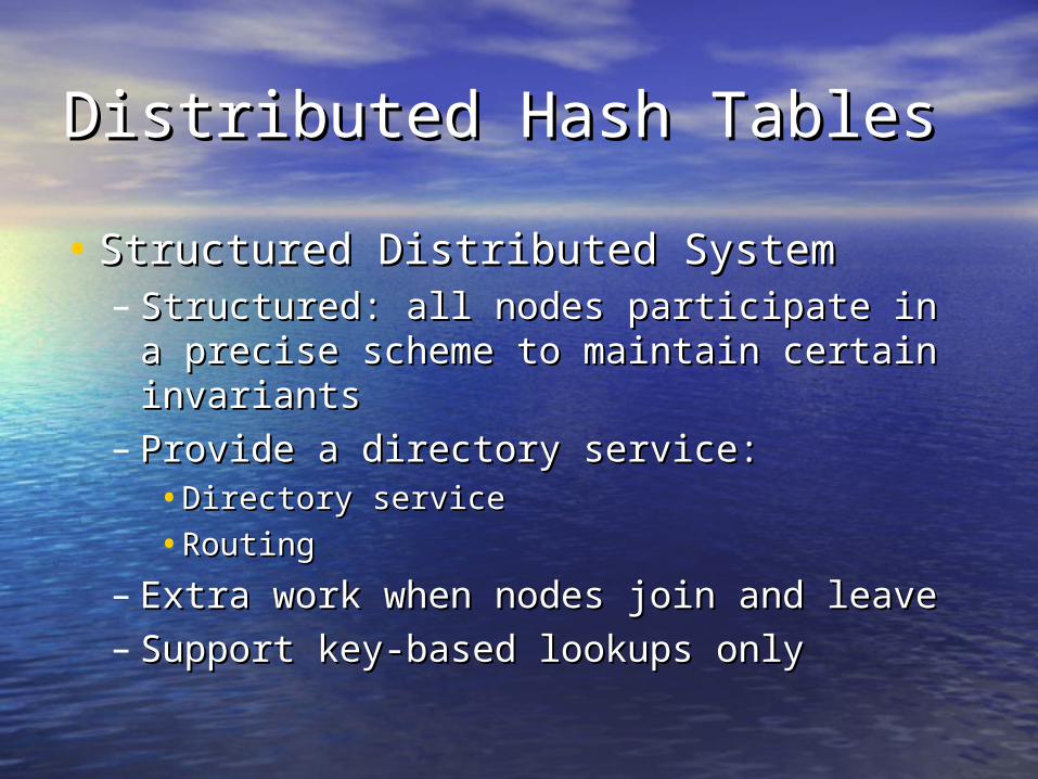
• Structured Distributed SystemStructured Distributed System– Structured: all nodes participate in a Structured: all nodes participate in a
precise scheme to maintain certain precise scheme to maintain certain invariantsinvariants
– Provide a directory service: Provide a directory service: •Directory serviceDirectory service
•RoutingRouting
– Extra work when nodes join and leaveExtra work when nodes join and leave– Support key-based lookups onlySupport key-based lookups only

BitTorrentBitTorrent
• Distribution of very large filesDistribution of very large files
• Tracker connects peers to each otherTracker connects peers to each other
• Peers exchange file blocks with each Peers exchange file blocks with each otherother
• Use Tit-for-Tat to discourage free Use Tit-for-Tat to discourage free loadingloading

Improving GnutellaImproving Gnutella
Gnutella-Style SystemsGnutella-Style Systems
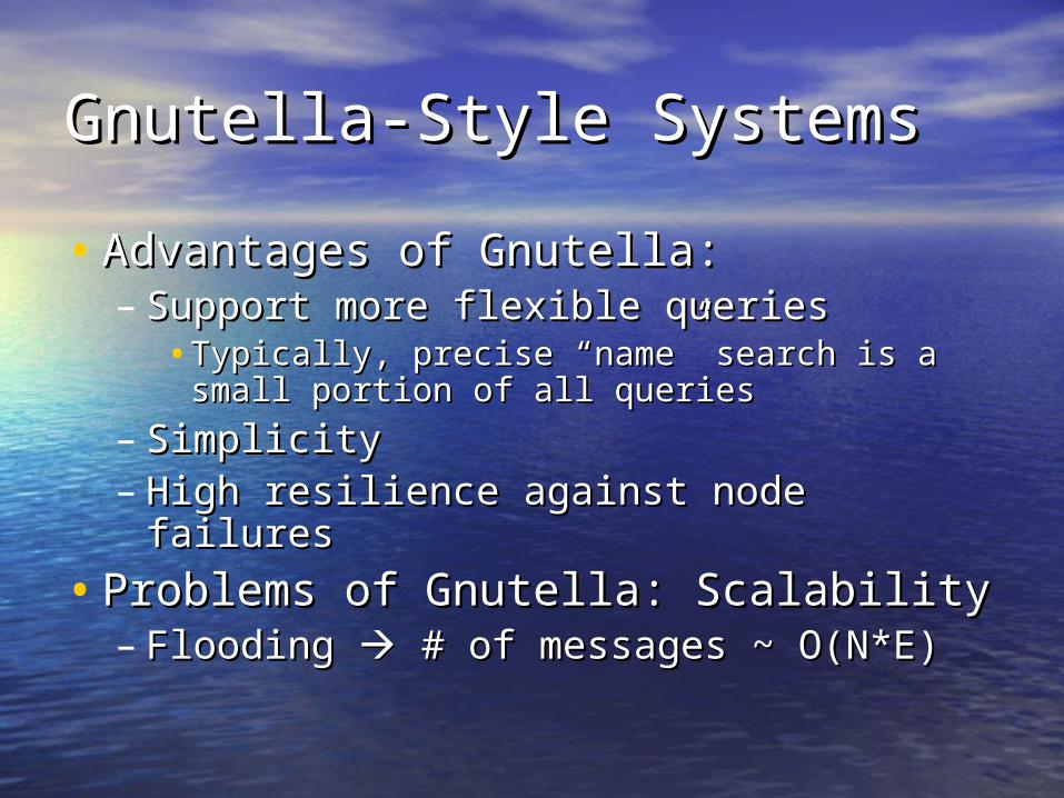
• Advantages of Gnutella: Advantages of Gnutella: – Support more flexible queriesSupport more flexible queries
•Typically, precise “name” search is a small Typically, precise “name” search is a small portion of all queriesportion of all queries
– SimplicitySimplicity– High resilience against node failuresHigh resilience against node failures
• Problems of Gnutella: ScalabilityProblems of Gnutella: Scalability– Flooding Flooding # of messages ~ O(N*E) # of messages ~ O(N*E)
Flooding-Based SearchesFlooding-Based Searches
. . . . . . . . . . . .
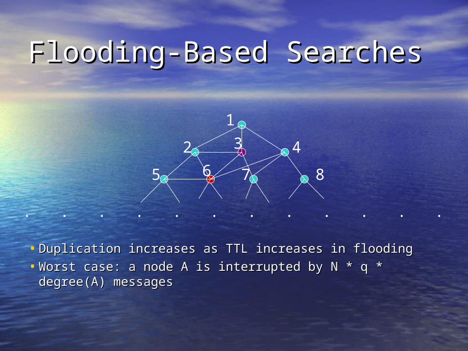
• Duplication increases as TTL increases in floodingDuplication increases as TTL increases in flooding
• Worst case: a node A is interrupted by N * q * Worst case: a node A is interrupted by N * q * degree(A) messagesdegree(A) messages
1
2 3 4
5 6 7 8
Load on Individual NodesLoad on Individual Nodes
• Why is a node interrupted:Why is a node interrupted:– To process a queryTo process a query– To route the query to other nodesTo route the query to other nodes– To process duplicated queries sent to itTo process duplicated queries sent to it
Communication ComplexityCommunication Complexity
Communication complexity Communication complexity determined by:determined by:
• Network topologyNetwork topology
• Distribution of object popularityDistribution of object popularity
• Distribution of replication density of Distribution of replication density of objectsobjects
Network TopologiesNetwork Topologies
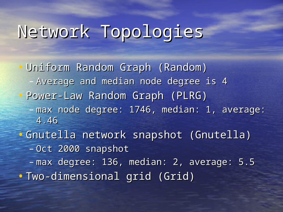
• Uniform Random Graph (Random)Uniform Random Graph (Random)– Average and median node degree is 4Average and median node degree is 4
• Power-Law Random Graph (PLRG)Power-Law Random Graph (PLRG)– max node degree: 1746, median: 1, average: max node degree: 1746, median: 1, average:
4.464.46
• Gnutella network snapshot (Gnutella)Gnutella network snapshot (Gnutella)– Oct 2000 snapshotOct 2000 snapshot– max degree: 136, median: 2, average: 5.5max degree: 136, median: 2, average: 5.5
• Two-dimensional grid (Grid)Two-dimensional grid (Grid)
Modeling MethodsModeling Methods
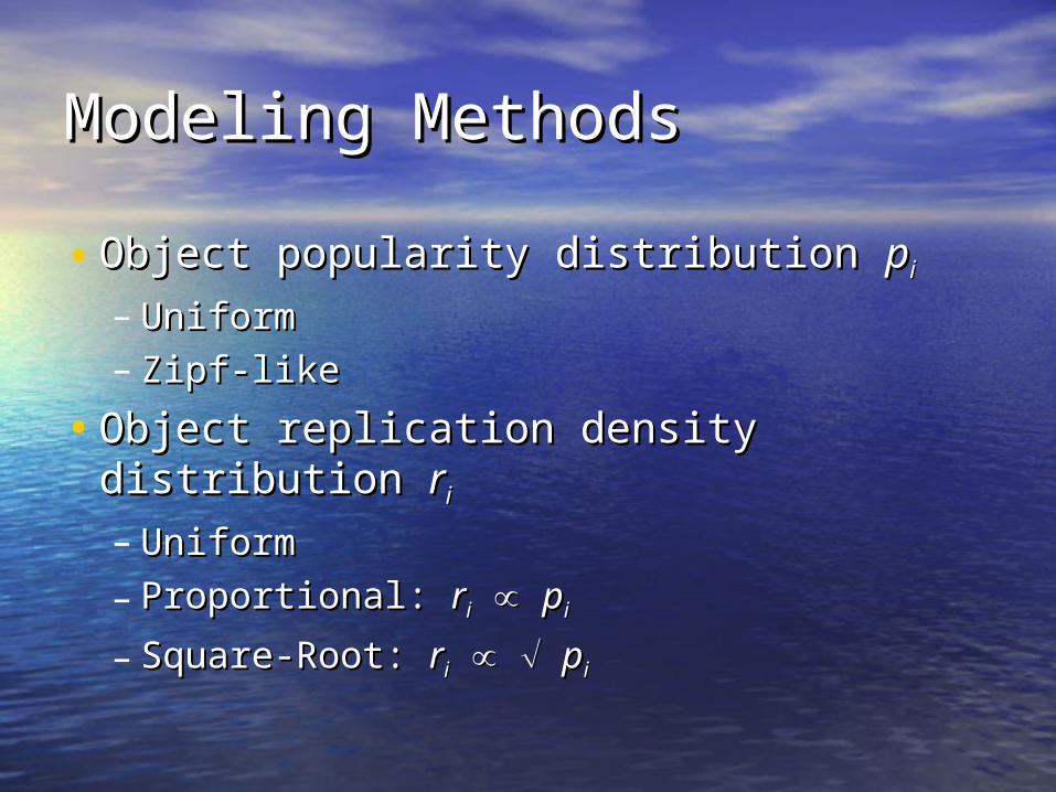
• Object popularity distribution Object popularity distribution ppii
– UniformUniform– Zipf-likeZipf-like
• Object replication density distribution Object replication density distribution rrii
– UniformUniform
– Proportional: Proportional: rrii ppii
– Square-Root: Square-Root: rrii ppii
Evaluation MetricsEvaluation Metrics
• Overhead: average # of messages Overhead: average # of messages per node per queryper node per query
• Probability of search success: Probability of search success: Pr(success)Pr(success)
• Delay: # of hops till successDelay: # of hops till success
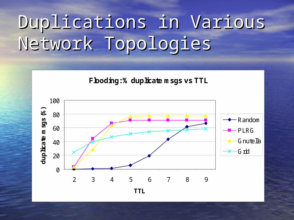
Duplications in Various Duplications in Various Network TopologiesNetwork Topologies
Flooding: % duplicate msgs vs TTL
0
20
40
60
80
100
2 3 4 5 6 7 8 9
TTL
du
pli
cate
msg
s (%
)
Random
PLRG
Gnutella
Grid
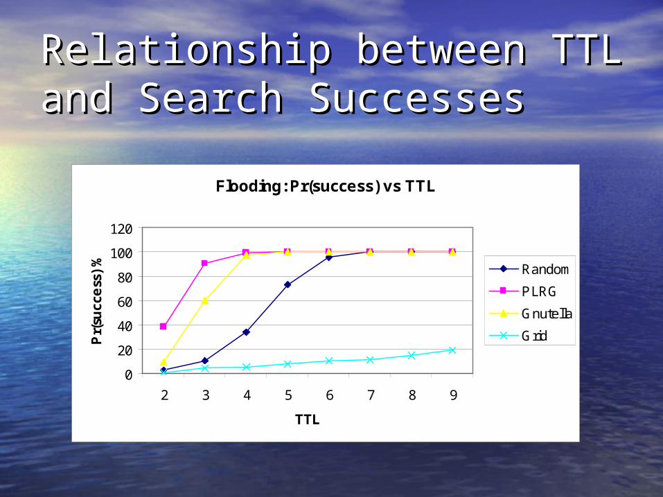
Relationship between TTL Relationship between TTL and Search Successesand Search Successes
Flooding: Pr(success) vs TTL
0
20
40
60
80
100
120
2 3 4 5 6 7 8 9
TTL
Pr(
succ
ess
) % Random
PLRG
Gnutella
Grid
Problems with Simple TTL-Problems with Simple TTL-Based FloodingBased Flooding
• Hard to choose TTL:Hard to choose TTL:– For objects that are widely present in For objects that are widely present in
the network, small TTLs sufficethe network, small TTLs suffice– For objects that are rare in the network, For objects that are rare in the network,
large TTLs are necessarylarge TTLs are necessary
• Number of query messages grow Number of query messages grow exponentially as TTL growsexponentially as TTL grows
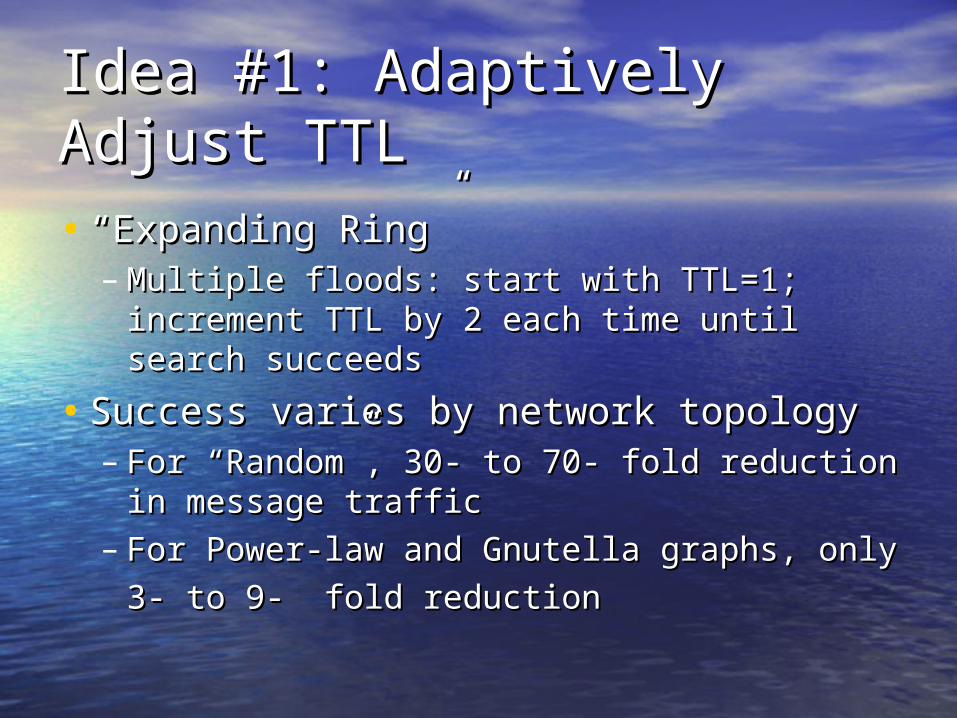
Idea #1: Adaptively Adjust Idea #1: Adaptively Adjust TTLTTL• ““Expanding Ring”Expanding Ring”
– Multiple floods: start with TTL=1; Multiple floods: start with TTL=1; increment TTL by 2 each time until search increment TTL by 2 each time until search succeedssucceeds
• Success varies by network topologySuccess varies by network topology– For “Random”, 30- to 70- fold reduction in For “Random”, 30- to 70- fold reduction in
message trafficmessage traffic– For Power-law and Gnutella graphs, only For Power-law and Gnutella graphs, only
3- to 9- fold reduction3- to 9- fold reduction
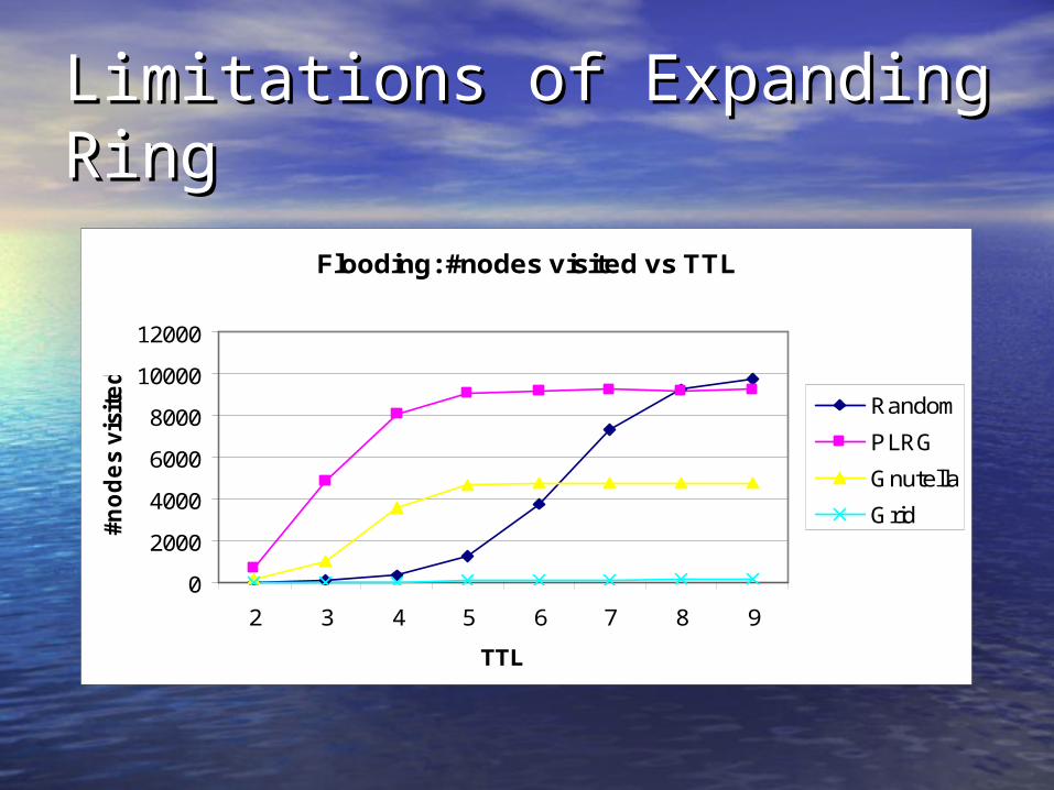
Limitations of Expanding Limitations of Expanding RingRing
Flooding: #nodes visited vs TTL
0
2000
4000
6000
8000
10000
12000
2 3 4 5 6 7 8 9
TTL
#n
od
es
vis
ite
d
Random
PLRG
Gnutella
Grid
Idea #2: Random WalkIdea #2: Random Walk
• Simple random walkSimple random walk– takes too long to find anything!takes too long to find anything!
• Multiple-walker random walkMultiple-walker random walk– N agents after each walking T steps visits N agents after each walking T steps visits
as many nodes as 1 agent walking N*T as many nodes as 1 agent walking N*T stepssteps
– When to terminate the search: check back When to terminate the search: check back with the query originator once every C with the query originator once every C stepssteps
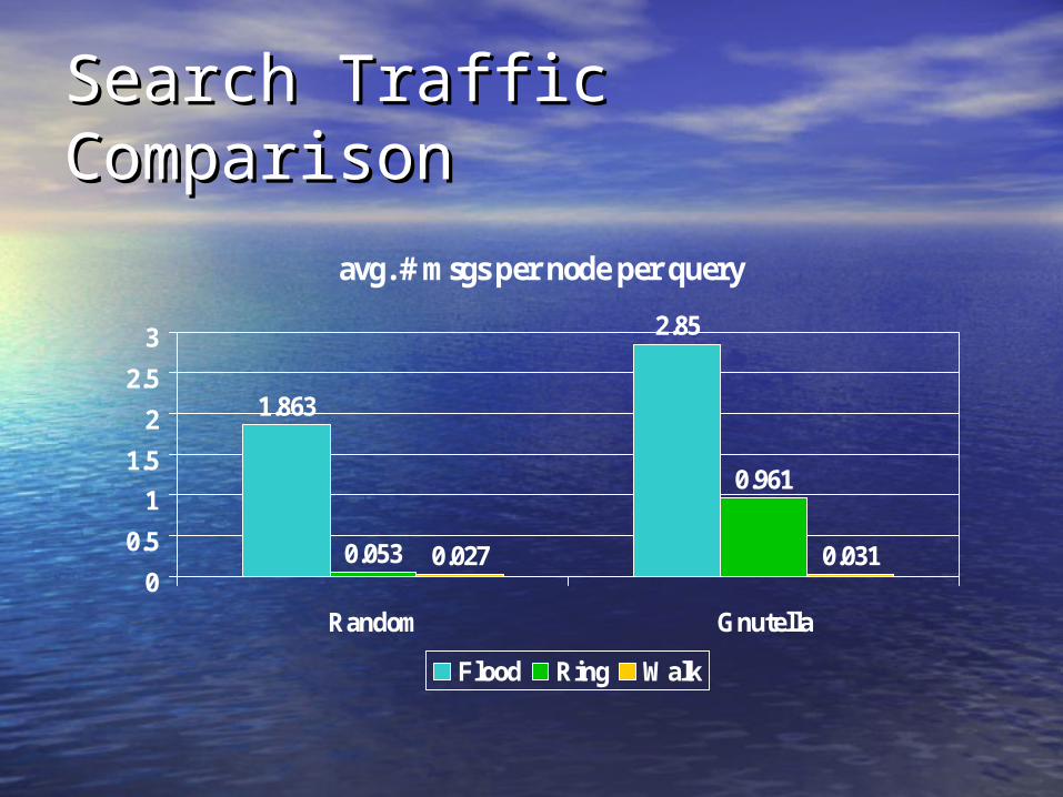
Search Traffic ComparisonSearch Traffic Comparison
avg. # msgs per node per query
1.863
2.85
0.053
0.961
0.027 0.0310
0.5
1
1.5
2
2.5
3
Random Gnutella
Flood Ring Walk
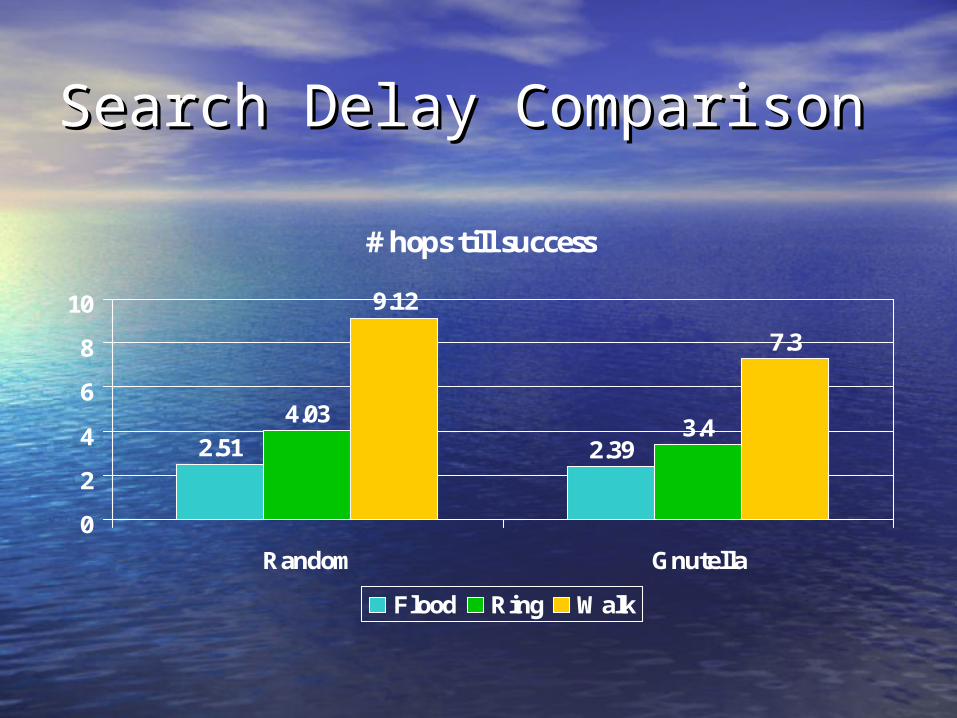
Search Delay ComparisonSearch Delay Comparison
# hops till success
2.51 2.39
4.033.4
9.12
7.3
0
2
4
6
8
10
Random Gnutella
Flood Ring Walk
Flexible ReplicationFlexible Replication
• In unstructured systems, search success is In unstructured systems, search success is essentially about coverage: visiting enough essentially about coverage: visiting enough nodes to probabilistically find the object nodes to probabilistically find the object => replication density matters=> replication density matters
• Limited node storage => what’s the Limited node storage => what’s the optimal replication density distribution?optimal replication density distribution?– In Gnutella, only nodes who query an object In Gnutella, only nodes who query an object
store it => store it => rrii ppii
– What if we have different replication strategies? What if we have different replication strategies?

Optimal rOptimal rii Distribution Distribution
• Goal: minimize Goal: minimize ( ( ppii/ / rri i ), where ), where rri i =R=R
• Calculation: Calculation: – introduce Lagrange multiplier introduce Lagrange multiplier , find , find rrii and and
that minimize: that minimize:
( ( ppii/ / rri i ) + ) + * ( * ( rri i - R)- R)
=> => - - ppii/ / rrii2 2 = 0 = 0 for all ifor all i
=> => rrii ppii
Square-Root DistributionSquare-Root Distribution
• General principle: to minimize General principle: to minimize ( ( ppii/ / rri i ) under constraint ) under constraint rri i =R, make =R, make rri i proportional to square root of proportional to square root of ppii
• Other application examples:Other application examples:– Bandwidth allocation to minimize Bandwidth allocation to minimize
expected download timesexpected download times– Server load balancing to minimize Server load balancing to minimize
expected request latencyexpected request latency
Achieving Square-Root Achieving Square-Root DistributionDistribution• Suggestions from some heuristicsSuggestions from some heuristics
– Store an object at a number of nodes that is Store an object at a number of nodes that is proportional to the number of node visited in proportional to the number of node visited in order to find the objectorder to find the object
– Each node uses random replacementEach node uses random replacement
• Two implementations:Two implementations:– Path replication: store the object along the Path replication: store the object along the
path of a successful “walk”path of a successful “walk”– Random replication: store the object randomly Random replication: store the object randomly
among nodes visited by the agentsamong nodes visited by the agents
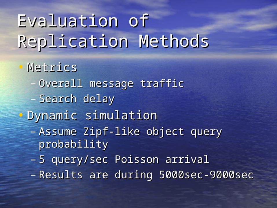
Evaluation of Replication Evaluation of Replication MethodsMethods
• MetricsMetrics– Overall message trafficOverall message traffic– Search delaySearch delay
• Dynamic simulationDynamic simulation– Assume Zipf-like object query Assume Zipf-like object query
probabilityprobability– 5 query/sec Poisson arrival5 query/sec Poisson arrival– Results are during 5000sec-9000secResults are during 5000sec-9000sec
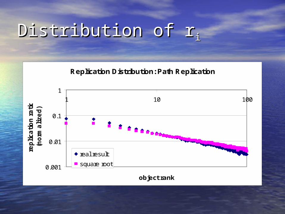
Distribution of rDistribution of rii
Replication Distribution: Path Replication
0.001
0.01
0.1
1
1 10 100
object rank
rep
lica
tio
n r
ati
o
(no
rma
lize
d)
real result
square root
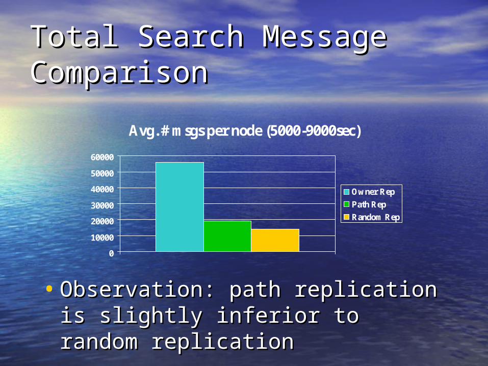
Total Search Message Total Search Message ComparisonComparison
• Observation: path replication is Observation: path replication is slightly inferior to random slightly inferior to random replicationreplication
Avg. # msgs per node (5000-9000sec)
0
10000
20000
30000
40000
50000
60000
Owner Rep
Path Rep
Random Rep
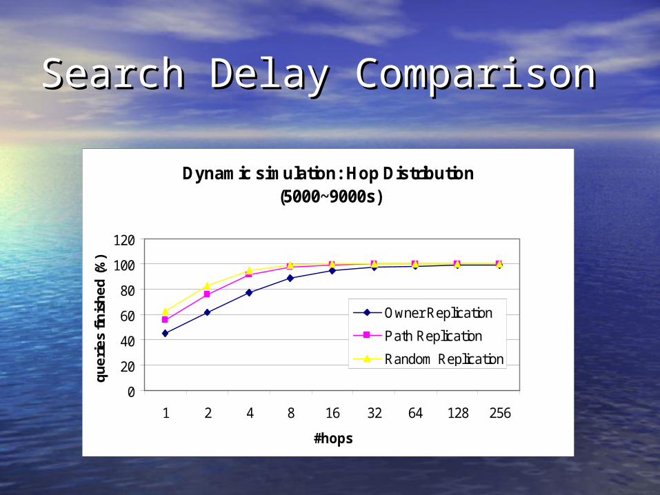
Search Delay ComparisonSearch Delay Comparison
Dynamic simulation: Hop Distribution (5000~9000s)
0
20
40
60
80
100
120
1 2 4 8 16 32 64 128 256
#hops
qu
eri
es
fin
ish
ed
(%
)
Owner Replication
Path Replication
Random Replication
Summary Summary
• Multi-walker random walk scales Multi-walker random walk scales much better than floodingmuch better than flooding– It won’t scale as perfectly as structured It won’t scale as perfectly as structured
network, but current unstructured network, but current unstructured network can be improved significantlynetwork can be improved significantly
• Square-root replication distribution is Square-root replication distribution is desirable and can be achieved via desirable and can be achieved via path replicationpath replication
KaZaaKaZaa
• Use SupernodesUse Supernodes
• Regular Nodes : Supernodes = 100 : Regular Nodes : Supernodes = 100 : 11
• Simple way to scale the system by a Simple way to scale the system by a factor of 100factor of 100

DHTs: A Brief OverviewDHTs: A Brief Overview(Slides by Bard Karp)(Slides by Bard Karp)
What Is a DHT?What Is a DHT?
• Single-node hash table:Single-node hash table:key = Hash(name)key = Hash(name)
put(key, value)put(key, value)
get(key) -> valueget(key) -> value
• How do I do this across millions of How do I do this across millions of hosts on the Internet?hosts on the Internet?– DistributedDistributed Hash Table Hash Table
Distributed Hash TablesDistributed Hash Tables
• ChordChord
• CANCAN
• PastryPastry
• TapastryTapastry
• etc. etc.etc. etc.
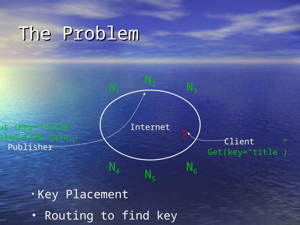
The ProblemThe Problem
Internet
N1
N2 N3
N6N5
N4
Publisher
Put (Key=“title”Value=file data…) Client
Get(key=“title”)
?
• Key Placement
• Routing to find key
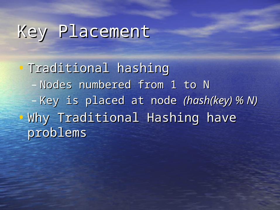
Key PlacementKey Placement
• Traditional hashingTraditional hashing– Nodes numbered from 1 to NNodes numbered from 1 to N– Key is placed at node Key is placed at node (hash(key) % N)(hash(key) % N)
• Why Traditional Hashing have Why Traditional Hashing have problemsproblems
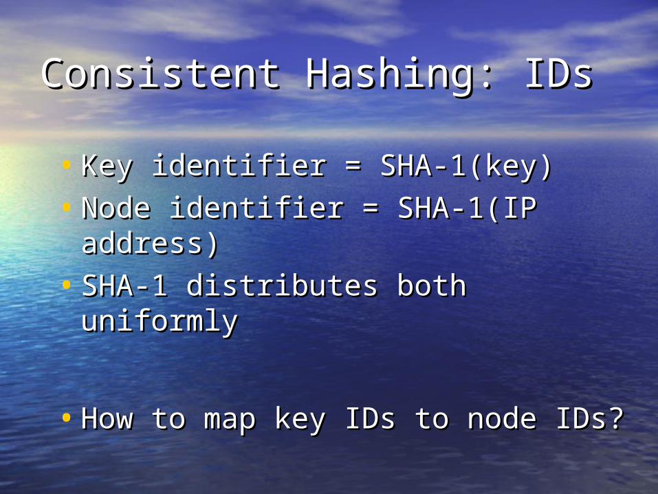
Consistent Hashing: IDsConsistent Hashing: IDs
• Key identifier = SHA-1(key)Key identifier = SHA-1(key)
• Node identifier = SHA-1(IP address)Node identifier = SHA-1(IP address)
• SHA-1 distributes both uniformlySHA-1 distributes both uniformly
• How to map key IDs to node IDs?How to map key IDs to node IDs?
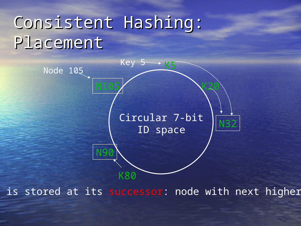
Consistent Hashing: PlacementConsistent Hashing: Placement
A key is stored at its successor: node with next higher ID
K80
N32
N90
N105 K20
K5
Circular 7-bitID space
Key 5Node 105

Basic LookupBasic Lookup
N32
N90
N105
N60
N10N120
K80
“Where is key 80?”
“N90 has K80”

““Finger Table” Allows log(N)-Finger Table” Allows log(N)-time Lookupstime Lookups
N80
½¼
1/8
1/161/321/641/128

Finger Finger ii Points to Successor of Points to Successor of n+2n+2ii
N80
½¼
1/8
1/161/321/641/128
112
N120
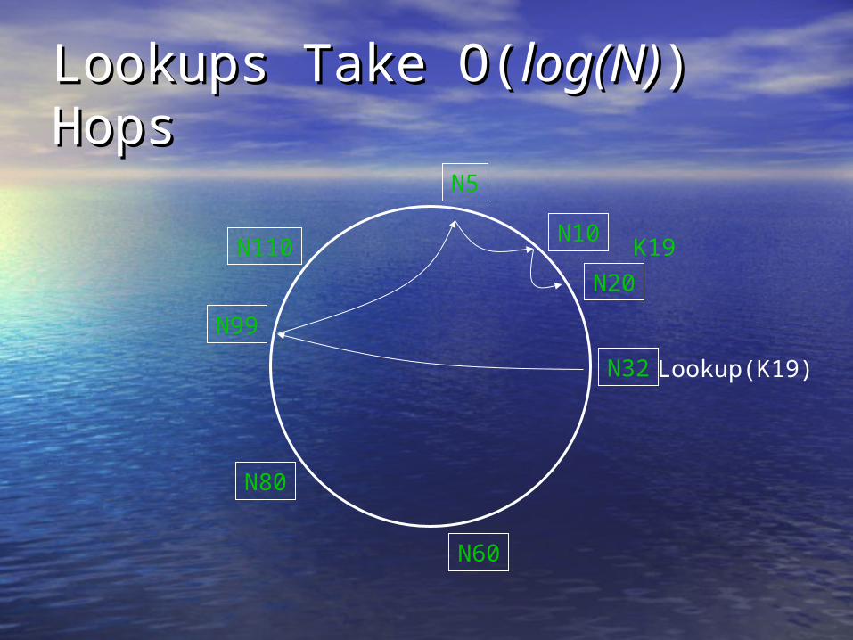
Lookups Take O(Lookups Take O(log(N)log(N)) Hops) Hops
N32
N10
N5
N20
N110
N99
N80
N60
Lookup(K19)
K19

Joining: Linked List InsertJoining: Linked List Insert
N36
N40
N25
1. Lookup(36)K30K38

Join (2)Join (2)
N36
N40
N25
2. N36 sets its ownsuccessor pointer
K30K38

Join (3)Join (3)
N36
N40
N25
3. Copy keys 26..36from N40 to N36
K30K38
K30
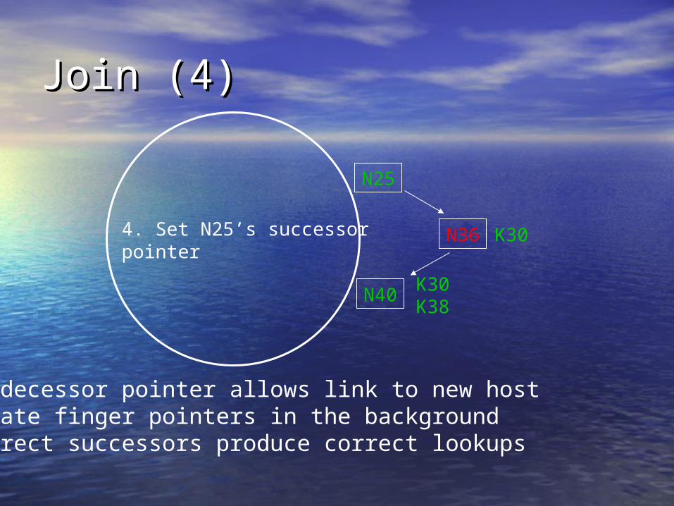
Join (4)Join (4)
N36
N40
N25
4. Set N25’s successorpointer
Predecessor pointer allows link to new hostUpdate finger pointers in the backgroundCorrect successors produce correct lookups
K30K38
K30
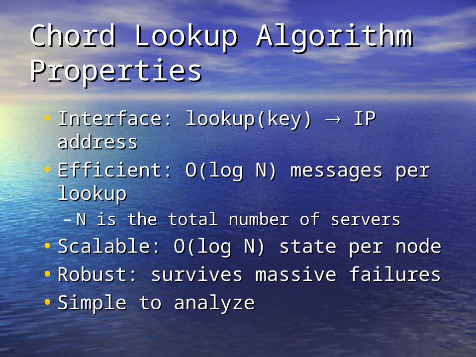
Chord Lookup Algorithm Chord Lookup Algorithm PropertiesProperties
• Interface: lookup(key) Interface: lookup(key) IP address IP address
• Efficient: O(log N) messages per Efficient: O(log N) messages per lookuplookup– N is the total number of serversN is the total number of servers
• Scalable: O(log N) state per nodeScalable: O(log N) state per node
• Robust: survives massive failuresRobust: survives massive failures
• Simple to analyzeSimple to analyze

Many Many Variations of The Many Many Variations of The Same ThemeSame Theme
• Different ways to choose the fingersDifferent ways to choose the fingers
• Ways to make it more robustWays to make it more robust
• Ways to make it more network Ways to make it more network efficientefficient
• etc. etc.etc. etc.

Improving BitTorrentImproving BitTorrent
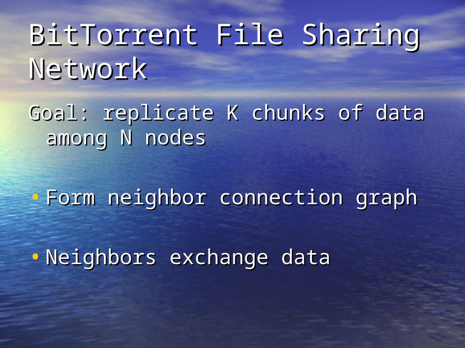
BitTorrent File Sharing BitTorrent File Sharing NetworkNetwork
Goal: replicate K chunks of data Goal: replicate K chunks of data among N nodesamong N nodes
• Form neighbor connection graphForm neighbor connection graph
• Neighbors exchange dataNeighbors exchange data
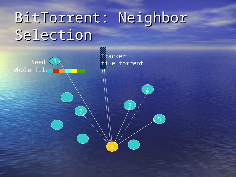
BitTorrent: Neighbor BitTorrent: Neighbor SelectionSelection
Trackerfile.torrent1Seed
Whole file
A
52
3
4
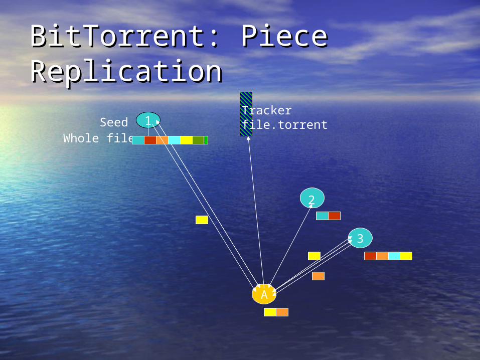
BitTorrent: Piece ReplicationBitTorrent: Piece Replication
Trackerfile.torrent1Seed
Whole file
A
3
2
BitTorrent: Piece Replication BitTorrent: Piece Replication AlgorithmsAlgorithms
• ““Tit-for-tat” (choking/unchoking):Tit-for-tat” (choking/unchoking):– Each peer only uploads to 7 other peers at a timeEach peer only uploads to 7 other peers at a time– 6 of these are chosen based on amount of data 6 of these are chosen based on amount of data
received from the neighbor in the last 20 secondsreceived from the neighbor in the last 20 seconds– The last one is chosen randomly, with a 75% bias The last one is chosen randomly, with a 75% bias
toward new comerstoward new comers
• (Local) Rarest-first replication:(Local) Rarest-first replication:– When peer 3 unchokes peer A, A selects which When peer 3 unchokes peer A, A selects which
piece to downloadpiece to download
Performance of BitTorrentPerformance of BitTorrent
• Conclusion from modeling studies: Conclusion from modeling studies: BitTorrent is nearly optimal in BitTorrent is nearly optimal in idealized, homogeneous networksidealized, homogeneous networks– Demonstrated by simulation studiesDemonstrated by simulation studies– Confirmed by theoretical modeling Confirmed by theoretical modeling
studiesstudies• Intuition: in a random graph, Intuition: in a random graph,
Prob(Peer A’s content is a subset of Peer B’s) ≤ Prob(Peer A’s content is a subset of Peer B’s) ≤ 50%50%
Lessons from BitTorrentLessons from BitTorrent
• Often, randomized simple algorithms Often, randomized simple algorithms perform better than elaborately perform better than elaborately designed deterministic algorithmsdesigned deterministic algorithms
Problems of BitTorrentProblems of BitTorrent
• ISPs are unhappyISPs are unhappy– BitTorrent is notoriously difficult to BitTorrent is notoriously difficult to
“traffic engineer”“traffic engineer”– ISPs: different links have different ISPs: different links have different
monetary costsmonetary costs– BitTorrent: BitTorrent:
•Peers are all equalPeers are all equal•Choices made based on measured Choices made based on measured
performanceperformance•No regards for underlying ISP topology or No regards for underlying ISP topology or
preferencespreferences
BitTorrent and ISPs: Play BitTorrent and ISPs: Play Together?Together?
• Current state of affairs: a clumsy co-Current state of affairs: a clumsy co-existenceexistence– ISPs “throttle” BitTorrent traffic along high-cost ISPs “throttle” BitTorrent traffic along high-cost
linkslinks– Users sufferUsers suffer
• Can they be partners?Can they be partners?– ISPs inform BitTorrent of its preferencesISPs inform BitTorrent of its preferences– BitTorrent schedules traffic in ways that benefit BitTorrent schedules traffic in ways that benefit
both Users and ISPsboth Users and ISPs
Random Neighbor SelectionRandom Neighbor Selection
• Existing studies all assume random Existing studies all assume random neighbor selectionneighbor selection– BitTorrent no longer optimal if nodes in BitTorrent no longer optimal if nodes in
the same ISP only connect to each otherthe same ISP only connect to each other
• Random neighbor selection Random neighbor selection high high cross-ISP trafficcross-ISP traffic
Q: Can we modify the neighbor selection Q: Can we modify the neighbor selection scheme without affecting scheme without affecting performance?performance?
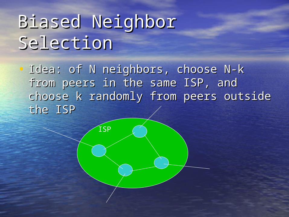
Biased Neighbor SelectionBiased Neighbor Selection
• Idea: of N neighbors, choose N-k from Idea: of N neighbors, choose N-k from peers in the same ISP, and choose k peers in the same ISP, and choose k randomly from peers outside the ISPrandomly from peers outside the ISP
ISP
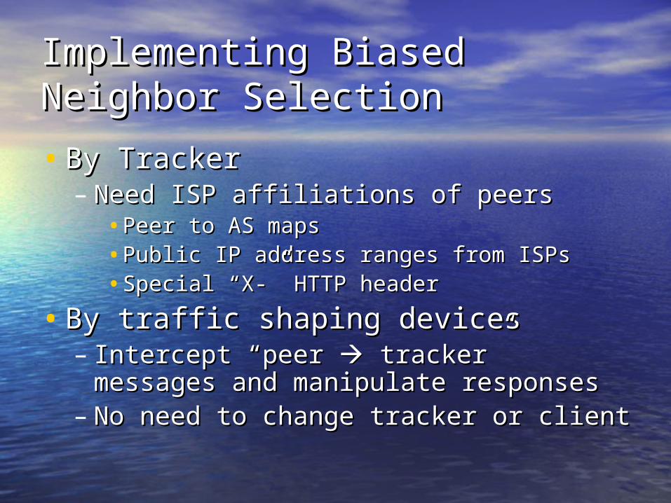
Implementing Biased Neighbor Implementing Biased Neighbor SelectionSelection
• By TrackerBy Tracker– Need ISP affiliations of peersNeed ISP affiliations of peers
•Peer to AS mapsPeer to AS maps•Public IP address ranges from ISPsPublic IP address ranges from ISPs•Special “X-” HTTP headerSpecial “X-” HTTP header
• By traffic shaping devicesBy traffic shaping devices– Intercept “peer Intercept “peer tracker” messages tracker” messages
and manipulate responsesand manipulate responses– No need to change tracker or clientNo need to change tracker or client
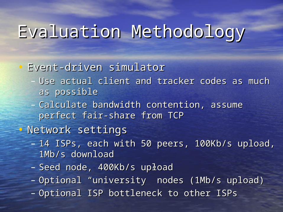
Evaluation MethodologyEvaluation Methodology
• Event-driven simulatorEvent-driven simulator– Use actual client and tracker codes as much as Use actual client and tracker codes as much as
possiblepossible– Calculate bandwidth contention, assume perfect Calculate bandwidth contention, assume perfect
fair-share from TCPfair-share from TCP
• Network settingsNetwork settings– 14 ISPs, each with 50 peers, 100Kb/s upload, 1Mb/s 14 ISPs, each with 50 peers, 100Kb/s upload, 1Mb/s
downloaddownload– Seed node, 400Kb/s uploadSeed node, 400Kb/s upload– Optional “university” nodes (1Mb/s upload)Optional “university” nodes (1Mb/s upload)– Optional ISP bottleneck to other ISPsOptional ISP bottleneck to other ISPs
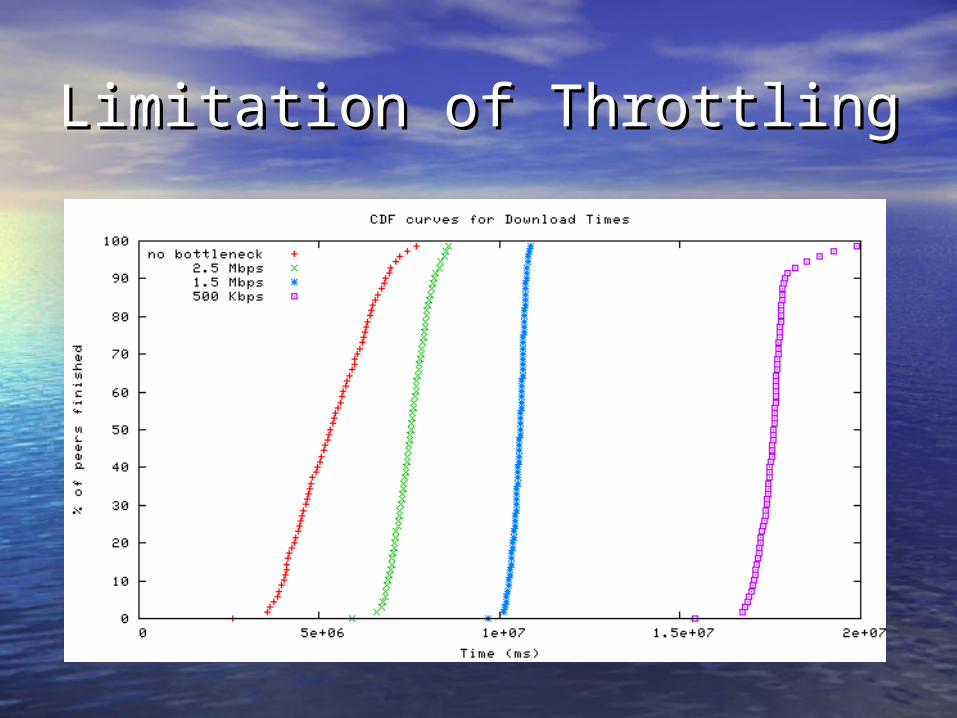
Limitation of ThrottlingLimitation of Throttling
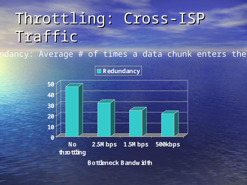
Throttling: Cross-ISP TrafficThrottling: Cross-ISP Traffic
0
10
20
30
40
50
Nothrottling
2.5Mbps 1.5Mbps 500kbps
Bottleneck Bandwidth
Redundancy
Redundancy: Average # of times a data chunk enters the ISP
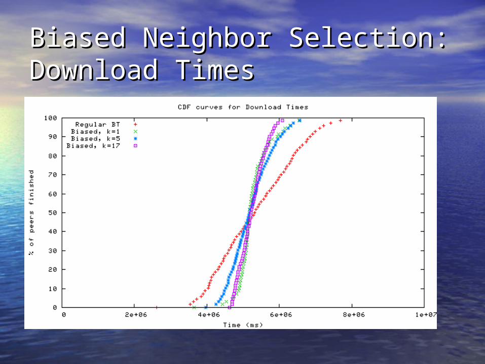
Biased Neighbor Selection: Biased Neighbor Selection: Download TimesDownload Times
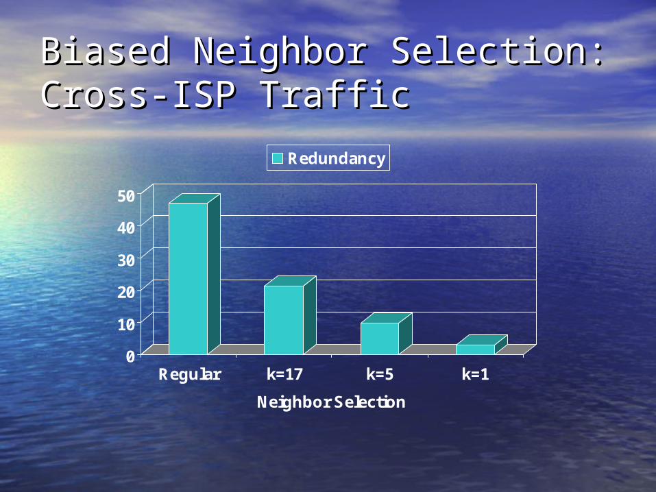
Biased Neighbor Selection: Biased Neighbor Selection: Cross-ISP TrafficCross-ISP Traffic
0
10
20
30
40
50
Regular k=17 k=5 k=1
Neighbor Selection
Redundancy
Importance of Rarest-First Importance of Rarest-First ReplicationReplication
• Random piece replication performs Random piece replication performs badlybadly– Increases download time by 84% - 150%Increases download time by 84% - 150%– Increase traffic redundancy from 3 to 14Increase traffic redundancy from 3 to 14
• Biased neighbors + Rarest-First Biased neighbors + Rarest-First More uniform progress of peersMore uniform progress of peers
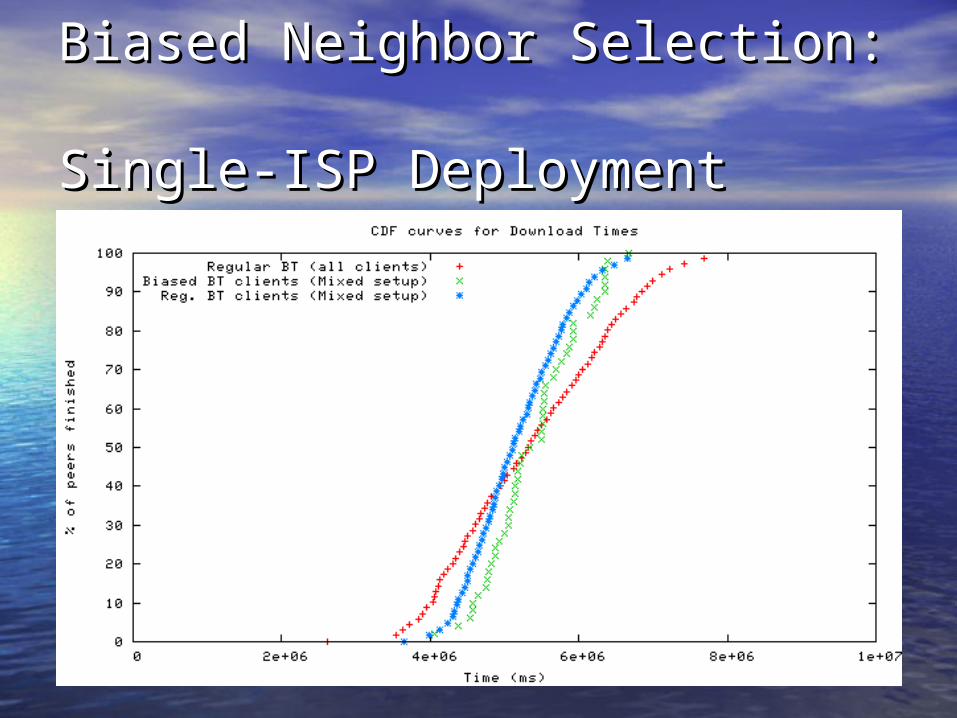
Biased Neighbor Selection: Biased Neighbor Selection: Single-ISP DeploymentSingle-ISP Deployment
Presence of External High-Presence of External High-Bandwidth PeersBandwidth Peers
• Biased neighbor selection alone: Biased neighbor selection alone: – Average download time same as regular Average download time same as regular
BitTorrentBitTorrent– Cross-ISP traffic increases as # of “university” Cross-ISP traffic increases as # of “university”
peers increasepeers increase• Result of tit-for-tatResult of tit-for-tat
• Biased neighbor selection + Throttling: Biased neighbor selection + Throttling: – Download time only increases by 12%Download time only increases by 12%
• Most neighbors do not cross the bottleneckMost neighbors do not cross the bottleneck
– Traffic redundancy (i.e. cross-ISP traffic) same Traffic redundancy (i.e. cross-ISP traffic) same as the scenario without “university” peersas the scenario without “university” peers
Comparison with Comparison with AlternativesAlternatives• Gateway peer: only one peer connects to Gateway peer: only one peer connects to
the peers outside the ISPthe peers outside the ISP– Gateway peer must have high bandwidthGateway peer must have high bandwidth
• It is the “seed” for this ISPIt is the “seed” for this ISP
– Ends up benefiting peers in other ISPsEnds up benefiting peers in other ISPs
• Caching:Caching:– Can be combined with biased neighbor selectionCan be combined with biased neighbor selection– Biased neighbor selection reduces the Biased neighbor selection reduces the
bandwidth needed from the cache by an order bandwidth needed from the cache by an order of magnitudeof magnitude
SummarySummary
• By choosing neighbors well, BitTorrent By choosing neighbors well, BitTorrent can achieve high peer performance can achieve high peer performance without increasing ISP costwithout increasing ISP cost– Biased neighbor selection: choose initial Biased neighbor selection: choose initial
set of neighbors wellset of neighbors well– Can be combined with throttling and Can be combined with throttling and
cachingcaching
P2P and ISPs can collaborate!P2P and ISPs can collaborate!