Evolution of Modern Business Cycle Models:

Accounting for the Great Recession

Patrick J. Kehoe Stanford University, University College London, and

Federal Reserve Bank of Minneapolis

Virgiliu Midrigan New York University

Elena Pastorino Stanford University, Hoover Institution,

and Federal Reserve Bank of Minneapolis

Staff Report 566 June 2018

DOI: https://doi.org/10.21034/sr.566 Keywords: New Keynesian models; Financial frictions; External validation JEL classification: E13, E32, E52, E61

The views expressed herein are those of the authors and not necessarily those of the Federal Reserve Bank of Minneapolis or the Federal Reserve System. __________________________________________________________________________________________

Federal Reserve Bank of Minneapolis • 90 Hennepin Avenue • Minneapolis, MN 55480-0291 https://www.minneapolisfed.org/research/

Evolution of Modern Business Cycle Models: Accounting

for the Great Recession∗

Patrick J. Kehoe† Virgiliu Midrigan‡ Elena Pastorino§

June 2018

Abstract

Modern business cycle theory focuses on the study of dynamic stochastic general equilibrium

models that generate aggregate fluctuations similar to those experienced by actual economies. We

discuss how this theory has evolved from its roots in the early real business cycle models of the late

1970s through the turmoil of the Great Recession four decades later. We document the strikingly

different pattern of comovements of macro aggregates during the Great Recession compared to

other postwar recessions, especially the 1982 recession. We then show how two versions of the

latest generation of real business cycle models can account, respectively, for the aggregate and the

cross-regional fluctuations observed in the Great Recession in the United States.

∗We thank Adrien Auclert, Mark Gertler, Robert Hall, Gordon Hanson, Robert Lucas, Ellen McGrattan, Juan Pablo

Nicolini, John Taylor, and Timothy Taylor for their comments, and are especially thankful to John Cochrane for his detailed

feedback. The views expressed herein are those of the authors and not necessarily those of the Federal Reserve Bank of

Minneapolis or the Federal Reserve System.†Stanford University, University College London, and Federal Reserve Bank of Minneapolis.‡New York University.§Stanford University, Hoover Institution, and Federal Reserve Bank of Minneapolis.

1

Modern business cycle theory focuses on the study of dynamic stochastic general equilibrium mod-

els that generate aggregate fluctuations similar to those experienced by actual economies. We discuss

how this theory has evolved across three generations, from its roots in the early real business cycle

models of the late 1970s through the turmoil of the Great Recession four decades later.

The first generation of these modern business cycle models were real business cycle models. They

primarily explored whether a small number of shocks, often one or two, could generate fluctuations sim-

ilar to those observed in aggregate variables such as output, consumption, investment, and hours. These

simple models disciplined their key parameters with micro evidence and were remarkably successful in

matching these aggregate variables.

Over time, as the theory evolved and computational possibilities expanded, a second generation of

these models appeared. These models incorporated frictions such as sticky prices and wages, and were

primarily developed to be used in central banks for short-term forecasting purposes and for performing

counterfactual policy experiments. Due to the focus on forecasting, the main emphasis in choosing

the parameters of these models was on their ability to match the behavior of, say, 10 to 12 aggregate

variables rather than on carefully matching them up with micro evidence. Although these models were

called New Keynesian, they had little to do with traditional Keynesian models. Rather, they were simply

real business cycle models augmented with sticky prices and wages. Indeed, a canonical real business

cycle model augmented with money and flexible prices—so that monetary policy can be meaningfully

discussed—has essentially the same implications for the importance of various shocks for business

cycles and nearly identical implications for optimal monetary and fiscal policy as these New Keynesian

models do.

During the last decade or so, macroeconomists working on the next generation of models have ben-

efited from the development of new algorithms and the increase in computing power to incorporate

the rich heterogeneity of patterns from the micro data even in models where no aggregation to a rep-

resentative firm or consumer is feasible. A defining characteristic of these models, though, is neither

the heterogeneity among model agents they accommodate nor the micro-level evidence they rely on,

although both are common, but rather the insistence that any new parameters or feature included be

explicitly disciplined by direct evidence. The spirit of the discipline of the parameters of these third-

1

generation models echoes the attitudes of the original developers of first-generation models, except that

third-generation models are sophisticated enough to match a wealth of additional aspects of the micro

data. The growth of such third-generation models was hastened by the Great Recession, a striking

episode that led macroeoconomists to dig more deeply than before into the links between disruptions in

the process of financial intermediation and business cycles.

In the final sections of the paper, we show how two versions of this latest generation of modern

business cycle models with frictions in labor and financial markets can account, respectively, for the

aggregate and the cross-regional fluctuations observed in the United States during the Great Recession.

We begin with a comparison of the comovements of the major macro aggregates in the two largest

post-war recessions in the United States: the 1982 recession, which exhibited essentially no financial

distress, and the Great Recession, which was characterized by the greatest distress of any post World

War II business cycle. In the 1982 recession, the drop in measured total factor productivity was as

large as the drop in output, whereas hours fell much less than output, which amounts to a pattern that

holds up across most postwar recessions. The pattern of these variables in the Great Recession was,

instead, strikingly different: measured total factor productivity barely fell, whereas labor fell more than

output. We argue that this fundamental difference in the pattern of comovements of output, measured

productivity, and hours in the Great Recession, along with the documented increase in financial distress,

calls for new mechanisms to explain this downturn.

Along with these specific examples, our overall message is that the basic questions that macro-

economists address have not changed over time, but rather that the development of real business cycle

methods has fundamentally changed how these questions are posed and answered. Now, we no longer

ask, “What is the best policy action we can take today?” but instead ask, “How does the behavior of

the economy considered compare under one rule for policy versus another rule for policy?” We answer

these questions with models that are specified at a deep enough level that their primitive features are

plausibly invariant to the policy exercises of interest, as well as shown to be consistent with a wealth of

relevant micro evidence.

Of course, macroeconomists still hold widely divergent views about the answers to fundamental

questions such as the ability of a well-specified rule for monetary policy to single-handedly stop an

2

incipient Great Depression episode in its tracks. But we now agree that a disciplined debate of such

questions rests on communication in the language of a dynamic general equilibrium model specified

at the level of primitives and internally as well as externally validated. Through such a disciplined

communication, we can reduce endless debates about opinions to concrete ones about the evidence for

detailed mechanisms and parameters.

1 First Generation: Basic Real Business Cycle Models

Modern business cycle models were developed in response to the Lucas critique of large-scale econo-

metric models built along traditional Keynesian lines, which were the dominant scientific paradigm in

macroeconomics from the 1950s to the 1970s. Lucas (1976) argued that unless an econometric model is

built at a deep enough level so that its parameters are invariant to the class of policy interventions being

considered, the model is of no value in assessing policy interventions, regardless of how well the model

performs in unconditional forecasting. The reason is that the policy intervention may affect key para-

meters that are presumed to be constant, and so invalidate the policy exercise. This critique motivated

macroeconomists to micro-found their dynamic models by building them starting from the specification

of technology, preferences, and other primitive constraints, along with an equilibrium concept. In the

resulting equilibrium, agents think intertemporally, not just statically, and decisions on consumption,

investment, and labor supply must simultaneously satisfy resource constraints and budget constraints.

From a practical viewpoint, this Keynesian macroeconometric framework fell out of favor after the

period of stagflation that many developed economies experienced during the 1970s. The reason is that

this framework offered neither a cohesive theoretical explanation for this stagflation episode nor, in

light of the Lucas critique, defensible policy advice.

1.1 Early Attempts to Match Aggregate Macro Variables

The first generation of modern business cycle models consisted of simple, primarily real business cycle

models with a representative consumer and few frictions, which were used to examine the extent to

which a small number of shocks, say, one or two, could account for the movements of major aggre-

gates, such as output, consumption, investment, and hours. In this framework, all economic behavior

3

was derived from one general equilibrium model, in which agents adjust their behavior when policies,

specified as rules, are changed, and forecast the future using the true probability distributions implied

by the model. A prominent example of such a model is in Prescott (1986), which features a represen-

tative consumer, one real exogenous technology shock, frictionless markets, and no money or nominal

variables. Earlier versions of first-generation business cycle models by Kydland and Prescott (1982)

and Long and Plosser (1983) featured much more complex real sides of the economy.

The early papers in this vein documented patterns in the macro data, typically summarized by a

table of moments of the data such as standard deviations, autocorrelations, and cross-correlations of

output, consumption, investment, hours, and a few other variables. This table, often referred to as a KP

table in light of Kydland and Prescott (1982), compared these moments in the data to those generated

by the model. Key discrepancies between the predictions of the model and the actual data were often

referred to as an “anomaly.” For example, a key anomaly of the early work was that hours in the models

fluctuated by less than half as much as in the data.

A typical research paper of this generation usefully focused on showing how adding one new mech-

anism to an otherwise standard model helped the model to better account for some existing anomaly.

Over time, the work evolved into the study of richer mechanisms. The work in this vein seriously

attempted to discipline new parameters with external evidence, which often involved connecting the

new parameters considered to those from micro studies. Nonetheless, the models were sufficiently sim-

ple that it was often difficult to tightly connect features or implications of new mechanisms with the

requisite evidence from micro-level data on consumers and firms.

The simple real business cycle models of that time with only stochastic movements in total factor

productivity generated fluctuations in the major aggregates largely in accord with those observed in the

data, when the technology parameter was simply taken as exogenous. As the Kydland and Prescott

(1982) paper makes abundantly clear, they were surprised that their simple model, which abstracted

from monetary frictions, could do so. However, this approach also gave rise to some oft-repeated

questions about their purpose and design which we discuss next.

4

1.2 Why Abstract from Money?

Why did early practitioners of the real business cycle approach focus on models that abstracted from

money and, hence, monetary policy? There are three reasons. First, the goal of this early work was to

develop the simplest possible model based on a coherent set of assumptions, in which agents acted in

their own self interest and that could produce fluctuations in aggregate quantities, such as output, con-

sumption, investment, and hours, broadly in accordance with those in the data. Second, the simplicity

of the models reflected existing limits on the ability to numerically compute these models. In the late

1970s, macroeconomists lacked the methods and computing power to solve complicated models with

heterogeneous agents, various frictions, and nonlinear effects. Third, many of the macroeconomists

working on real business cycles were deeply affected by the failures of the policy advice derived from

the earlier statistical Keynesian models that helped to exacerbate the stagflation of the 1970s. Hence,

they retreated to a humbler intellectual position focused on building coherent foundations for macro-

economics and avoiding both the Lucas critique and the hubris that led to previous mistakes. Most

macroeconomists felt quite uncomfortable rushing back to the policy arena without well-developed

models.

Sometimes it is thought that the most important reason why real business cycle modelers abstracted

from money was because they believed that monetary policy has no effect on the real economy. (See,

for example, Summers 1986 and Romer 2016.) We argue that this view is incorrect. Part of the mis-

understanding seems to have arisen from the well-known policy ineffectiveness proposition of Sargent

and Wallace (1975). Sargent and Wallace articulated a critique of models that produced real effects of

money solely because agents were assumed to be irrational.

In a similar vein, Barro (1977) critiques “sticky wage” models. He argues that even if nominal wages

do not vary with monetary shocks, if we model wages and employment levels as part of a contract that

is mutually agreed upon by firms and workers, then there is no room for monetary feedback rules to

systematically improve outcomes. Barro points out a weak theoretical link in a popular mechanism:

even if sticky nominal wages are assumed, existing models generate real effects solely because they

assume that the employment contract does not specify hours worked in addition to wages and so leaves

5

unexploited mutual gains from trade.

Properly understood, both Sargent and Wallace (1975) and Barro (1977) were critiques of popular

existing mechanisms for monetary nonneutrality rather than the expression of either a belief that no co-

herent model could be developed in which monetary policy had real effects or that in actual economies

monetary policies have no real effects. For example, there is near-universal agreement that the disas-

trous monetary policies pursued by countries such as Argentina, Brazil, and Chile had serious adverse

effects on these economies.

More broadly, macroeconomists agree on the direction in which monetary policy should respond to

shocks over the cycle—although they disagree on the magnitude of desirable monetary interventions.

Even with a general agreement on how monetary policy works in a qualitative sense, it remains an

exceptionally difficult task to build a coherent model in which consumers and firms act in their own

self-interest and that quantitatively captures well how monetary policy works. For instance, as Barro

(1977) foresaw, the difficulty with many of the sticky wage or price models is that they rely on agents

agreeing to contracts that ignore mutual gains for trade. At a deeper level, the fact that a contract in

such models is not optimal given preferences, technology, and information makes them subject to the

Lucas critique. Our own sense is that depending on the exact standard that needs to be met before the

word coherent is applicable, macroeconomists may still be a decade or two away from achieving that

goal of having a coherent model.

1.3 Why Focus on Technology Shocks?

Real business cycle models are driven by what are commonly referred to as technology shocks. Why did

early researchers choose to treat the aggregate productivity parameter in the output production function

as the key stochastic variable? There are two practical reasons. First, productivity is relatively easy to

measure, given a functional form assumption for the aggregate production function, data on aggregate

output, the capital stock, and hours. Second, with a single shock added nearly anywhere else in a

one-sector growth model, it is difficult to generate the business cycle comovements between output,

consumption, investment, and hours found in the data.

For example, a shock that primarily leads to a deep fall in investment tends to make consumption

6

and investment move in opposite directions, which is inconsistent with the data. To see why, consider

the effect of a fall in investment on output. Since the capital stock is over 10 times investment, a drop

in investment has only a tiny effect on the capital stock and no direct effect on labor, so the amount

produced with capital and labor barely moves. But from the resource constraint, consumption and in-

vestment must add up to output. Hence, the only way that investment can fall a lot, output barely move,

and the resource constraint be satisfied is for consumption to rise. Using a quantitative model, Cooper

and Ejarque (2000) show that shocks that operate through an investment channel counterfactually imply

that consumption and investment are negatively correlated.

Consider next a shock that reduces the desire to work and, hence, reduces hours. With a Cobb-

Douglas aggregate production technology and a labor share of two-thirds, a given percentage drop in

hours, say 10 percent, leads to only two-thirds (6.7 percent) as large a drop in output. But if such

shocks are the main drivers of the business cycle, then labor would be much more volatile than output,

an implication that is inconsistent with US business cycles prior to the Great Recession. (See Chari,

Kehoe, and McGrattan 2007 and Brinca, Chari, Kehoe, and McGrattan 2016.)

Finally, it is also important to understand how this time-varying aggregate productivity parameter

should be interpreted. From the beginning of modern business cycle theory, it was well accepted that

movements in this parameter should not be interpreted as changes in “technology.” That is, falls in

measured total factor productivity should not be thought of as individual firms forgetting how to produce

or deteriorations in the blueprints at the firm level for turning capital and labor into output. Rather, the

time variation of the productivity parameter has always been thought of as a stand-in for deeper models

of how economic outputs and inputs adjust to various nonproductivity shocks.

For one example, Lagos (2006) shows that in a standard search model with only firm-level produc-

tivity differences, an increase in either employment subsidies or costs of firing workers decreases the

cutoff for how productive an individual firm must be in order to operate. Hence, these policies lead the

average productivity of firms to fall and, hence, lead to a fall in total factor productivity. For another

example, Chari et al. (2007) consider an increase in input financing frictions across sectors in that in

bad times in some sectors, the cost of borrowing rises relative to that in other sectors. This financing

friction distorts the mix of each sector’s input in final output and hence gives rise to measured falls in

7

total factor productivity.

An alternative view is that neither of these approaches is necessary to understand drops in measured

total factor productivity because this measured drop mostly disappears if we simply adjust for the fall

in capital utilization, uKt, in downturns. To see how this argument works, let uKtKt be the service

flow from the capital stock, Kt, and Yt = At(uKtKt)αL1−αt be a Cobb-Douglas production function.

Clearly, drops in uαKt show up as drops in total factor productivity.

The challenge for this view is to provide a micro-founded reason for utilization to fall steeply

enough during recessions to account for the measured fall in total factor productivity. The problem

is that given that the vast bulk of a firm’s expenses is for labor, keeping the capital stock running is

typically much less expensive than paying for labor. Hence, quantitatively relevant micro-founded

models often imply very modest declines in capital utilization during downturns. Moreover, since the

capital share is small, say, α = 25 percent, such falls in capital utilization can account for only a very

small fraction of the measured fall in total factor productivity. Of course, if in the data firms actually

drastically reduce their capital utilization in recessions, then the puzzle is to explain why they do so.

More theoretical work needs to be done in this area for progress to be made.

2 Second Generation: For Central Banks with a New Keynesian

Twist

The second generation of modern business cycle models consisted of medium-scale dynamic stochas-

tic general equilibrium models, which were nearly all of the New Keynesian variety and much more

complex than those of the first generation. The development of these models was driven by a desire

from central banks around the world to find a practical replacement for the earlier large-scale Keyne-

sian models. As a result, this new generation of medium-scale New Keynesian models needed to be

conceived in a way that money could have real effects and be sophisticated enough that they could be

used for forecasting.

These second-generation models were designed to fit the behavior of 10 or so aggregate time series

that include output, consumption, investment, hours, and some nominal variables such as inflation and

nominal interest rates. Because the metric for success in these models was their ability to reproduce

8

the behavior of these aggregates, most of the effort in those models was expended on adding additional

features—such as one shock per equation, nonstandard adjustment costs, and extra parameters in pref-

erences and technology—that allowed the model to fit in-sample properties of these aggregates. Little

effort was devoted to ensuring that the added shocks, especially the unobservable ones, were clearly

interpretable and that the added parameters were disciplined by an explicit attempt to validate them. In

practice, these models featured such a complex mix of competing mechanisms, frictions, and shocks

that they were quite difficult to understand. In this sense, the methodology for building and assessing

second-generation models diverged sharply from that of first-generation models.

A more fundamental methodological issue with these second-generation models that deeply divides

macroeconomists is how to build a model that is not subject to the Lucas critique. In practice, this means

we need to ask, “What is a primitive enough level at which to specify a model so that the resulting

model is arguably invariant to the policy interventions of interest?” For first-generation modelers, this

level consists of technologies, including commitment technologies, preferences, information structure,

and physical constraints, such as capital adjustment costs. After these objects are specified, agents are

free to choose the contracts to sign or the assets to trade, subject to these primitive frictions. Second-

generation modelers, instead, appended direct restrictions on contracts, such as particular forms of

sticky wage contracts or restrictions on the class of asset trades allowed, even though these restrictions

are not in anyone’s interest given the primitive frictions.

For example, a second-generation model may assume that private contracts cannot depend on ob-

servable variables outside of any single agent’s control, such as aggregate output, and then argue that

such a restriction justifies government intervention in the form of a state-contingent tax policy to par-

tially restore the effective insurance not provided by private contracts. From the point of view of a

first-generation modeler, this approach is problematic, since the government intervention may affect

the unspecified premise of why certain behavior is infeasible and so give rise to perverse incentives or

unintended undesirable consequences. For example, if the true reason such a private contingent contract

is infeasible is that it violates an unspecified incentive constraint, then the uncontingent contract that is

made contingent by the government policy also violates the same unspecified incentive constraint. (For

an early exposition of a version of this view, see Barro 1977.)

9

These new models are often presented as essentially traditional Keynesian models derived from

maximizing behavior, which has led to some confusion. Even though the labels IS and LM are often

attached to certain equations, it is crucial to understand that these second-generation modern business

cycle models are built on the first-generation models, not on the Keynesian IS-LM model. That is, the

New Keynesian models are simply real business cycle models with a few frictions added on. Thus, al-

though it may be surprising to nonmacroeconomists, a canonical real business cycle model, augmented

with money and flexible prices so that monetary policy can be meaningfully discussed, has essentially

the same implications for the fraction of business cycle fluctuations explained by various shocks and,

perhaps more surprisingly, the same implications for policy as a canonical New Keynesian model.

To see that real business cycle models and New Keynesian models both imply that technology

shocks account for the vast bulk of fluctuations, consider two models. On the one hand, we have a

classic real business cycle model by Prescott (1986). He compares the variance of detrended output in

his model to the variance of detrended US output, and documents that 70 percent of the variance of the

observed fluctuations in output in the US economy can be mechanically accounted for by productivity

shocks (p. 16). On the other hand, using a state-of-the-art New Keynesian model, Justiniano, Primiceri,

and Tambalotti (2010) find that technology shocks, here the sum of neutral and investment-specific

technology shocks, account for 75 percent of the variance of output, which, somewhat surprisingly,

is actually a higher percentage than that in Prescott’s calculation.1 In sum, a typical New Keynesian

model added several frictions and shocks, but at its core, the key driving force for business cycles is

a real business cycle model. Indeed, in the state-of-the-art New Keynesian model by Justiniano et al.

(2010 p. 134), monetary policy shocks account for only a negligible fraction of the movements in

output. In short, a New Keynesian model is exactly as Justiniano et al. (2010 p. 134) describe: “It is a

medium-scale DSGE model with a neoclassical core, augmented with several frictions.”

In part, the belief that real business cycle and New Keynesian models are based on different sources

of economic fluctuations may represent a confusion about labeling. Some New Keynesian models

1We view this model as an updated version of the highly cited paper by Smets and Wouters (2007), which itself is a

descendant of the Christiano, Eichenbaum, and Evans (2005) paper. Briefly, Smets and Wouters (2007) exclude changes in

inventories from their definition of investment and include the purchases of consumer durables in consumption rather than

investment. Justiniano et al. (2010), instead, include both the change in inventories and the purchases of consumer durables

in investment. In other respects, the models are essentially identical.

10

like Smets and Wouters (2007) and Justiniano et al. (2010) refer to investment-specific technology

shocks as demand shocks, even though they represent shifts in the production function for the supply of

investment goods, which might naturally seem to be types of supply shocks. Given the possibility for

confusion on this point, these terms may have lost their usefulness.2

A second point is that under the popular narrative, New Keynesian models and flexible price models

have radically different implications for monetary policy: in New Keynesian models, activist monetary

policy is necessary to reduce the volatility of output and offset reductions in demand, whereas in flexible

price models, monetary policy has no such role. We contend that this narrative reflects a deep misunder-

standing of the workings and implications of these models. The genesis of this misunderstanding may

be traced to the way New Keynesian models were presented, namely as traditional Keynesian models

of the IS-LM variety but with maximizing agents.

This contention has been proven by Correia, Nicolini, and Teles (2008). These authors show that

the monetary and fiscal policy implications of a flexible price model and a standard New Keynesian

model in which prices are sticky are identical. The flexible price model is a real business cycle model

with essentially neutral money added on, in that money has little effect on output, in which consumers

can purchase some goods with cash obtained in advance and some other goods with credit—referred

to as a cash-credit cash-in-advance model. The model features stochastic productivity shocks and

stochastic government spending, as in Lucas and Stokey (1983), modified to have differentiated varieties

of a single consumption good sold by monopolistic competitors. The New Keynesian model is an

identical model except that prices are sticky in that producers are allowed to adjust their prices only at

random (Poisson) times. The set of instruments available to the government are the money supply (or

equivalently, nominal interest rates) and state-contingent linear taxes on consumption and labor income.

The main result is that in both models, it is optimal to have identical policies: constant (producer)

prices and set tax rates to smooth distortions by equating the relevant margins over time. Critically, if

an outside observer had data from this sticky price economy under such an optimal policy, fluctuations

2For another example in which this terminology is less than helpful, consider a constant elasticity of substitution demand

function for a differentiated product yd = (p/P )−θY , where p is the price of that product, P is the aggregate price index,

and Y is aggregate output. From the point of view of an individual producer, shifts in Y are shifts in that producer’s demand

curve, even when these shifts in Y come from aggregate productivity shocks. Here again, demand and supply terminology

is not helpful.

11

in all aggregates would be identical to those generated by a frictionless real business cycle model,

adjusted to include neutral money. The reason is that in the original sticky price economy, optimal

monetary policy is not attempting to offset real shocks to the economy, but instead is attempting to

reproduce the flexible price allocations of the frictionless version of the model.

An immediate corollary of the work of Correia et al. (2008) is that the zero lower bound constraint,

namely the constraint that nominal interest rates cannot be negative, has no impact on the equivalence

of policy in New Keynesian and flexible price models. Hence, when taxes are set optimally the idea that

the zero lower bound constraint makes increasing government spending more attractive than otherwise

does not hold either. (See Correia, Farhi, Nicolini, and Teles for details.)

Finally, it is commonly argued that it is interesting to deprive the government of nearly all fiscal

instruments when analyzing monetary policy because, in practice, it is difficult to quickly adjust fis-

cal policy in the depths of a recession. We argue that at least for deep recessions, this claim is not

true: witness the speed at which the Obama Stimulus program, formally, the American Recovery and

Reinvestment Act of 2009, was passed. Regardless of the merits of this program, it was clearly passed

quickly enough to affect the economic recovery.

In sum, New Keynesian models are most certainly not reincarnations of textbook IS-LM models

with maximization added on. Rather, they are real business cycle models augmented with a couple

of distortions—typically sticky prices and monopoly power—and shocks that do little to contribute to

fluctuations or influence the nature of optimal policy.

3 Third Generation: Matching Aggregate Time Series Combined

with External Validation

The goal of second-generation models, nearly all New Keynesian ones, was to help central banks in their

medium-term forecasting and allow central banks to use them for counterfactual policy experiments in

order to inform the policy debate. In contrast, the goal of third-generation models is to develop new and

more deeply founded mechanisms that formalize alternative possible explanations for business cycles as

well as provide convincing external validation for the quantitative importance of these newly formalized

mechanisms.

12

Indeed, the hallmark of the third generation of modern business cycle models is their focus on an

explicit external validation of their key mechanisms, using evidence independent of the particular ag-

gregate time series for which the model is designed to account. Many of these third-generation models

incorporate micro-level heterogeneity and are built on a tight connection between the mechanism in the

model and the wealth of micro-level data pertinent to the key forces in the model. A defining charac-

teristic of these models, though, is neither the heterogeneity among model agents they accommodate

nor the micro-level evidence they rely on, although both are common, but rather their insistence that

any new parameters or feature included be explicitly disciplined by direct evidence. In this sense, the

spirit of the discipline of third-generation models echoes the attitudes of the original developers of first-

generation models, except that third-generation models are sophisticated enough to match a wealth of

additional aspects of the micro data and, in contrast to the first-generation models, do not need to be

able to be aggregated to be solved.

More broadly, third-generation models grew naturally out of the first-generation ones. Third-

generation models have become feasible to explore only now because of the development of sophis-

ticated algorithms and the advent of high-powered computers to compute them. Several decades ago,

if a researcher was interested in a nonlinear model with both idiosyncratic and aggregate shocks, it was

necessary to make assumptions so that the heterogeneity could be aggregated back to a suitably defined

representative consumer and firm.

For example, in the classic model by Bernanke, Gertler, and Gilchrist (1999), even though banks

are heterogeneous in their net worth, the model aggregates in that the only state variable of banks that

needs to be recorded is aggregate net worth. The reason is that the model is carefully set up so that the

value functions are linear in net worth. With new algorithms and greater computing power, it is feasible

to compute such models even if they do not aggregate, so that the relevant aggregate state is the entire

distribution of net worth across firms.

Many observers thought that the Great Recession would have led to an upheaval in macroeconomic

modeling (for example, Christiano 2016). After all, these observers argued, much of the observed con-

traction in output was driven by disruptions in credit markets that spilled over into the real economy, but

nearly all business cycle models featured no such links between financial and real activity. We argue

13

that no upheaval ever happened: in contrast to the Great Stagflation of the 1970s, the Great Recession

had essentially no impact on macroeconomic methodology per se. Rather, the Great Recession sim-

ply prompted macroeconomists to design models that elevated financial frictions from their previously

modest role in amplifying the effects of other shocks, as in the classic work by Bernanke et al. (1999),

to playing a central role in amplifying the shocks generating downturns.3 The main consequence of the

Great Recession was to push macroeconomists further away from the medium-scale New Keynesian

models with hard-to-interpret shocks and frictions, chosen mainly for their ability to fit macro aggre-

gates, back to more elaborate versions of first-generation models of behavior modeled from primitives,

which are then internally disciplined and externally validated by looking at their detailed implications

for the data.

Although there are now many fine examples of third-generation models, below we discuss two

examples of third-generation work with which we are most familiar.4 In both examples, the use of

micro-level data is used to discipline the models’ new features and assess how the proposed mecha-

nisms are borne out in the relevant data on consumers and firms. The illustration in the next section

draws on the work of Arellano, Bai, and Kehoe (forthcoming), which is motivated both by micro-level

and macro-level patterns of firm behavior and by the Great Recession of 2007-2009, which we first

review. The illustration in the following section focuses on the work of Kehoe, Midrigan, and Pas-

torino (forthcoming), which is motivated by the challenge for business cycle models to account for the

cross-regional patterns of employment, consumption, and wages witnessed in the Great Recession.

Before reviewing these two examples, we compare the comovements of aggregates across the two

largest postwar US recessions: the 1982 one and the Great Recession.

3A vibrant literature in international macroeconomics had already developed open economy models that included fi-

nancial crises. However, the mechanisms explored in this work were not immediately applicable to the pattern of crises

witnessed in large developed economies such as the United States. The reason is that the patterns of crises in small emerg-

ing markets pointed to the central role of issues like a sudden stop of capital inflows (Mendoza 2010) and possible defaults

on sovereign debt (like Cole and Kehoe 2000; Arellano 2008; Neumeyer and Perri 2005). These issues are clearly relevant

to episodes in Argentina, Mexico, and Greece but they played essentially no role in the US Great Recession.4An important hybrid of second- and third-generation approaches is the work of Kaplan, Moll, and Violante (2018),

which incorporates heterogeneous consumers into a New Keynesian model. On the one hand, whereas the costs of pur-

chasing illiquid assets are disciplined by consumers’ responses to unanticipated tax rebates, the key features of the model,

namely the consumers’ heterogeneous responses to monetary shocks, are not disciplined by the data. Moreover, computa-

tional limitations force the authors to consider only one-time unanticipated shocks, so that the implications of the model for

business cycles are not yet known.

14

3.1 Classifying and Modeling Recessions: 1982 and the Great Recession

In terms of understanding and accounting for the Great Recession, two questions arise. First, can the

Great Recession be thought of as a financial recession in a way that earlier large recessions such as the

1982 recession cannot be? Second, do the patterns of comovement between, say, output, hours, and

productivity differ across financial and nonfinancial recessions?

To answer the first question, we draw on the work of Romer and Romer (2017), who argue that the

1982 recession in the United States exhibited no financial distress, whereas the Great Recession in the

United States displayed some of the greatest financial distress in the entire post-World War II sample

of developed countries. Romer and Romer (2017) construct a financial distress measure based on a

real-time narrative source, the OECD Economic Outlook, to identify the severity crisis by the size of

the change of various indicators, including increases in the costs to financial institutions in obtaining

funds and general increases in the perceived riskiness of financial institutions.

These authors show that throughout the entire 1982 recession, the distress measure for the United

States indicated their lowest possible level of distress, namely no distress. Throughout the Great Re-

cession, instead, this same measure indicates a growing level of distress that peaks in 2008 at a level

indicating extreme financial distress. These two recessions are then clean cases to compare for the

United States in terms of the comovements of macro aggregates, since they are the two deepest postwar

recessions the country experienced, and they display the opposite extremes in the amount of financial

distress.5

As panel A of Figure 1 shows, while the 1982 recession was somewhat deeper than the Great

Recession, the downturn following the Great Recession was much more persistent.6 The more basic

question is whether the patterns of comovements among the major aggregates differ between financial

5In terms of modeling financial distress, an important issue is that of reverse causation. Regardless of the underlying

cause, the deeper a recession is, the more likely that firms and households that contracted uncontingent loans will find it hard

to repay them and, hence, the more likely that the financial institutions that extended such loans will experience financial

distress. Moreover, the feedback is highly likely to go both ways: underlying causes, perhaps only partially financial,

generate financial distress, which, in the presence of financial frictions, exacerbate the real downturn and lead to more

distress. In short, an open question is whether the financial crisis is the result of a “shock” in the sense of a economy-wide

run on financial institutions or whether financial frictions amplify other shocks and, hence, give rise to severe financial

distress.6Some economists, such as Taylor (2016), argue that the causes of this slow growth are not directly connected to the

financial crisis that accompanied the Great Recession.

15

and nonfinancial recessions to the point where a different mechanism is called for that is different from

those that conventionally account for most of the other postwar recessions. The short answer is “yes.”

The comovements among output, hours, and total factor productivity in the Great Recession in the

United States differed from earlier recessions: compared to the 1982 recession, in the Great Recession

the drop in total factor productivity was much smaller relative to the drop in output, whereas the drop

in hours was much larger and longer-lasting than the drop in output. In terms of mechanisms, these pat-

terns imply that the 1982 recession was characterized by the typical pattern of most postwar recessions,

which can be mechanically accounted for by drops in total factor productivity, whereas the pattern in the

Great Recession cannot be. This latter recession, instead, seems to suggest the need for a mechanism

that makes labor fall much more relative to output than it does in both typical recessions and in standard

models. (See Brinca et al. 2016.)

As for the data, the two panels of Figure 2 illustrate this difference. In panel A, we graph output

detrended by a 1.6 percent trend and non-detrended hours, both normalized to 100 in 1979:Q1. We see

that, relative to 1979:Q1, output falls about 10 percent and hours falls about 6 percent so that the decline

in hours is much smaller than the decline in output. In panel B, we graph output for the Great Recession

detrended by a 1.6 percent trend, as well as non-detrended hours, both normalized to 100 in 2007:Q3.

Comparing the levels in 2007:Q3 to those in the subsequent trough, output falls about 7 percent and

hours falls about 9 percent. Critically, during the Great Recession the decline in hours is larger than the

decline in output. Since standard real business models imply that for any given productivitity shock,

the percentage fall in hours is less than half of that in output, such models simply cannot account for

the patterns of comovements in the Great Recession.

In sum, the 1982 recession, which exhibited no financial distress, was a typical real business cy-

cle recession.7 In contrast, the Great Recession, which exhibited financial distress that was an order

of magnitude larger than all other postwar US recessions, had a modest fall in measured total factor

productivity but a fall in hours greater than the fall in output.

7Note that as Chari et al. (2007) stress, since measured fluctuations in total factor productivity are best thought of as

efficiency wedges, namely, reduced-form shocks that arise from the interaction of frictions with primitive shocks, this finding

could be consistent with the view that the decline in measured total factor productivity was generated by a monetary policy

reaction to nontechnology shocks.

16

3.2 A Mechanism for the Patterns of Comovements during the Great Recession

3.2.1 Evidence for and Description of a New Mechanism

Any mechanism that accounts for the Great Recession must generate a large downturn in output asso-

ciated with a sharp fall in hours, must generate a small decline in measured productivity, and must also

be consistent with a large rise in measured financial distress.

One striking feature of the micro data on the Great Recession is that the financial crisis during the

Great Recession was accompanied by large increases in the cross-section dispersional of firm growth

rates (see Bloom, Floetotto, Jaimovich, Saporta-Eckstein, and Terry 2014). Indeed, as panel B of Figure

1 shows, the increase in the interquartile range of firms’ sales growth during the Great Recession was

nearly triple that during the 1982 recession. As credit conditions tightened during the financial crisis,

firms’ credit spreads increased, whereas both equity payouts and debt purchases decreased. Motivated

by these observations and the patterns of comovement described earlier, Arellano et al. (forthcoming)

build a model with heterogeneous firms and financial frictions, in which increases in volatility at the firm

level lead to increases in the cross-sectional dispersion of firm growth rates, a worsening of financial

conditions, and a decrease in aggregate output and labor associated with small movements in measured

total factor productivity.

The key idea in the model is that hiring inputs to produce output is risky: firms must hire inputs

before they receive the revenues from their sales. To hire these inputs, firms must pledge to use some of

their future revenues to pay for them. In this context, (owners of) a firm face the risk of any idiosyncratic

shock that occurs between the time of production and the receipt of revenues. When financial markets

are incomplete in that firms have only access to debt contracts to insure against such shocks, firms

and their creditors must bear this risk, which has real consequences if firms must experience a costly

default once they cannot meet their financial obligations. In the model, an increase in uncertainty

arising from an increase in the volatility of idiosyncratic productivity shocks at the firm level makes the

revenues from any given amount of labor hired more volatile and, thus, a default more likely. Thus, in

equilibrium an increase in volatility leads firms to hire fewer inputs.

The model features a continuum of heterogeneous firms that produce differentiated products. The

17

productivity of these firms is subject to idiosyncratic shocks with stochastically time-varying volatility;

these volatility shocks are the only aggregate shocks in the economy. Three ingredients are critical to

the workings of the model. First, firms hire their inputs—here, labor—and produce before they know

their idiosyncratic shocks. The insight that hiring labor is a risky investment is a hallmark of quantitative

search and matching models but is missing from most simple macroeconomic models. Second, financial

markets are incomplete in that firms have access only to state-uncontingent debt and can default on it.

Firms face interest rate schedules for borrowing that depend on all the shocks; higher borrowing and

labor hiring result in higher probabilities of default. Third, motivated by the work of Jensen (1986),

the model includes an agency friction in that managers can divert free cash flow to projects that benefit

themselves at the expense of firms. This friction makes it optimal for firms to limit free cash flow and,

by so doing, makes firms less able to self-insure against adverse shocks.

In the model, the main result is that an increase in uncertainty arising from an increase in the volatil-

ity of idiosyncratic productivity shocks increases the volatility of the revenues from any given amount

of labor hired. As the risk of default increases, firms cut back on hiring inputs. This result depends

critically on the assumptions of incomplete financial markets and the agency friction. If firms had ac-

cess to complete financial markets, firms would simply respond to a rise in volatility by restructuring

the pattern of payments across states and, as Arellano et al. (forthcoming) show, both output and labor

would increase sharply when volatility rises. Indeed, when the distribution of idiosyncratic productivity

spreads out and shocks are serially correlated, firms with high current productivity shocks tend to hire

relatively more of the factor inputs. It is only when the volatility of firm-level productivity shocks is

accompanied by financial frictions that the model produces a downturn in output. Without agency costs,

firms could self-insure by maintaining a large buffer stock of unused credit. Absent the agency friction,

firms find it optimal to build up buffer stocks well in excess of those observed in the data. With it,

however, find it optimal to limit the size of their buffer stocks and maintain debt levels consistent with

those in the data. With such debt levels the model generates realistic fluctuations in labor.

Quantitatively, the authors investigate whether an increase in the volatility of firm-level idiosyncratic

productivity shocks, which generates the increase in the cross-sectional dispersion of firm-level growth

rates observed in the recent recession, leads to a sizable contraction in aggregate economic activity

18

and tighter financial conditions. To do so, the authors choose a sequence of volatility shocks so that

the model produces the same cross-sectional increase in sales growth as observed during the Great

Recession. Figure 3A shows the resulting cross-sectional volatility of sales growth in the model and the

data, where the latter is measured by the interquartile range of sales growth across firms. Figures 3B

and 3C show that the model can account for essentially all of the contraction in output and labor that

occurred in the Great Recession. Figures 3D, 3E, and 3F show that the model also does a reasonable

job of reproducing the changes in financial variables that occurred during this period, as measured by

credit spreads, debt purchases, and equity payouts. More generally, Arellano et al. (forthcoming) show

that their model generates labor fluctuations that are large relative to those in output, similar to the

relationship between output and labor in the data.

3.2.2 Third-Generation Nature of the Exercise

It is useful to contrast the Arellano et al. (forthcoming) approach linking the model to the micro data

to that used in a well-cited second-generation approach to financial shocks and the Great Recession,

namely, that of Christiano, Motto, and Rostagno (2017). This latter paper focuses on fitting 12 aggregate

time series: GDP, consumption, investment, hours, inflation, wages, prices of investment goods, and

the federal funds rate as well as four aggregate financial variables. The Christiano et al. (2017) paper

represents the frontier work in that generation of work, but it never attempts to compare the detailed

patterns of firm-level variables implied by the model to those in the data.

In contrast, the paper by Arellano et al. (forthcoming) takes a very different approach to the micro

data. The authors start by showing that the model is consistent with some basic features of firms’

financial conditions over the cycle, namely that firm spreads are countercyclical, as in the data, and

that both the ratio of debt purchases to output and the ratio of equity payouts to output have similar

correlations with output and volatility as in the data.

They then turn to micro moments of financial variables from the cross-sectional distribution of

firms. Table 1 presents the time series median of spreads, the growth of sales, leverage, debt purchases,

and equity payouts by each quartile. While there are some differences, this very simple model does a

reasonable job of producing these moments. They also show that the correlations of firm-level leverage

with firm-level credit spreads, sales growth, debt purchases, and equity payouts are similar in the model

19

and the data.

3.3 A Mechanism for the Regional Patterns in the Great Recession

3.3.1 Evidence for and Description of a New Mechanism

An alternative and complementary insight into the Great Recession can be gained by exploring the

distinctively different regional characteristics of the Great Recession in the United States. To that end,

we first discuss the regional patterns of employment, consumption, and wages in the United States

during that time. We then conclude by presenting a promising mechanism that accounts for the strongly

differential response of different US states to the Great Recession.

During the Great Recession, the regions of the United States that experienced the largest declines

in household debt also experienced the largest drops in consumption, employment, and wages (see,

for example, Mian and Sufi 2011, 2014). Here, we focus on two main aggregate patterns. First, the

regions of the United States that were characterized by the largest declines in consumption were also

characterized by the largest declines in employment, especially in the nontradable goods sector. Second,

the regions that experienced the largest employment declines also experienced the largest declines in

real wages relative to trend.

The panels of Figure 4 summarize these patterns. Kehoe et al. (forthcoming) illustrate the first

pattern by using annual state-level data on employment and consumption from the Bureau of Economic

Analysis. In the spirit of the model, we isolate changes in consumption associated with changes in

households’ ability to borrow—or, more generally, in credit conditions—as proxied by changes in house

prices, by projecting state-level consumption growth on the corresponding growth in state-level (Zillow)

house prices. We use the resulting series for consumption growth in our analysis (for a similar approach,

see Charles, Hurst, and Notowidigdo 2015).

Panel A of Figure 4, taken from Kehoe et al. (forthcoming), plots state-level employment growth

between 2007 and 2009 against the measure of state-level consumption growth just described over this

same period. The elasticity of employment to consumption is 0.38. Panels B and C show that consump-

tion declines are associated with relatively large declines in nontradable employment and essentially

no changes in tradable employment across states: a 10 percent decline in consumption across states is

20

associated with a 5.5 percent decline in nontradable employment and a negligible (and statistically in-

significant) 0.3 percent increase in tradable employment. The large negative intercept in panel C shows

that the decline in tradable employment is sizable in all states but unrelated to changes in state-level

consumption.

The second main correlation is shown in panel D of Figure 4, which reproduces a version of the

findings in Beraja, Hurst, and Ospina (2016). These authors document that wages were moderately

flexible in the cross section of US regions: the cross-regional decline in wages was almost as large

as the decline in employment. We closely follow their approach by using census data for wages from

the Integrated Public Use Microdata Series, and controlling for observable differences in workforce

composition both across states and within a state over time, as in Beraja et al. (2016). As panel D

shows, a decline in employment of 10 percent across US states during the Great Recession is associated

with a decline in wages of 7.8 percent.

To investigate these cross-regional patterns, Beraja et al. (2016) use what they term a semi-structural

methodology, which uses a simple general equilibrium model together with a combination of regional

and aggregate data to identify the regional and aggregate shocks driving business cycles. In particular,

based on detailed census data at the household level on employment and wages, they find that, in the

cross section, in regions where hours worked fell relatively more, nominal and real wages fall relatively

more. These authors also show that shocks to the intertemporal marginal rate of substitution, called

discount factor shocks, can account for the vast bulk of the cross-regional variation in employment in

the United States during the Great Recession. The idea of using shocks to the discount factor as a proxy

for variations in financial risk in the context of the Great Recession was also used by Hall (2017).8

By developing an approach to exploring these cross-regional patterns that is complementary to

Beraja et al. (2016), Kehoe et al. (forthcoming) investigate how the interplay between credit and labor

market frictions can account for the cross-sectional patterns just documented. We develop a version of

the Diamond-Mortensen-Pissarides search model with risk-averse agents, borrowing constraints, and

human capital accumulation. The underlying idea is that hiring workers is an investment activity: costs

8Here we have discussed one class of models that accounts for aggregate movements and another that accounts for cross-

sectional movements. For an interesting model that attempts to account for both at the same time see Jones, Midrigan, and

Phillipon (2017).

21

of creating vacancies are paid up front, whereas benefits, as measured by the flows of surplus from the

match between a firm and worker, accrue over time. In this framework, a credit tightening generates a

fall in investment—including investment related to hiring workers—which induces firms to post fewer

vacancies and so causes employment in the aggregate to fall.

The key innovation here is the addition of human capital accumulation. In a textbook version of

the Diamond-Mortensen-Pissarides search model without human capital accumulation, a large fraction

of the present value of benefits from forming a match accrues early in the match. As a result, credit

tightening has little effect on hiring in this model. But in the presence of human capital accumulation,

the flows of benefits from forming a match have a much longer duration. Intuitively, a match not

only produces current output but also augments a worker’s human capital, with persistent effects on a

worker’s output flows (a finding that holds even if matches dissolve at a high rate). This significantly

longer duration of surplus flows, or returns to employment, amplifies the drop in employment from a

credit contraction, like the one observed during the Great Recession, by a factor of 10 relative to that

implied by the model without human capital accumulation.

To build intuition for our new mechanism, consider a firm’s incentives to post vacancies after a

credit tightening that leads to a temporary fall in consumption. Since consumers have a desire to smooth

consumption, this temporary fall in consumption increases consumers’ marginal utility and hence their

shadow price of current goods, which then mean-reverts. This temporary increase in the shadow price

of goods has two opposing effects. First, it increases the cost of posting vacancies by raising the shadow

value of the goods used in this investment. Second, it increases the surplus from a match by raising the

shadow value of the surplus flows produced by a match. The cost of posting vacancies rises by more

than the benefits because the cost of posting new vacancies is incurred immediately when goods are

especially valuable, whereas the benefits accrue gradually in the future when workers acquire human

capital with employment. As a result, firms post fewer vacancies, and in the aggregate employment

contracts. The longer is the duration of the surplus flows from a match, the larger is the resulting drop

in vacancies.

We show that the resulting model does an excellent job of reproducing the cross-state patterns in

terms of the comovement of consumption and nontradable employment, tradable employment, and

22

overall employment. The model is also consistent with the observation in Beraja et al. (2016) that

in the cross section of US states, wages are moderately flexible: a 10 percent drop in employment is

associated with a fall in wages of 7.8 percent in both the data and the model. Thus, the model predicts

sizable employment changes in response to a credit tightening, even though wages are as flexible as

they are in the data. As Beraja et al. (2016) emphasize, this finding of substantial wage flexibility in the

data casts doubt on the popular explanations of the Great Recession in the New Keynesian literature.

3.3.2 Third-Generation Nature of the Exercise

It is helpful to contrast second- and third-generation approaches to understand the cross-regional fea-

tures of the Great Recession discussed above.

The second-generation approach would simply imply choosing parameters for the human capital

process so as to fit the state-level employment patterns observed in the data, without informing this

choice with any specific micro evidence on the relationship between human capital accumulation and

wage growth or verifying whether the inferred parameters are consistent with additional micro evidence.

Instead we proceed as follows. Because the process for human capital accumulation is critical for

the model’s predictions, we take great care in using micro data to quantify it. The top part of Table

2 illustrates how we use cross-sectional differences in wages from Elsby and Shapiro (2012) on how

wages increase with experience and longitudinal data on how wages grow over an employment spell

from Buchinsky et al. (2010) to discipline the model parameters.

The bottom part of Table 2 shows how we used other evidence, not directly targeted in our moment-

matching exercise, to externally validate other features of the micro data. For example, we show that

the model produces drops in wages after a nonemployment spell, the sensitivity of this wage drop to

an additional year of tenure, the standard deviation of wages at the beginning of an employment spell,

and the profit share of revenue similar to the corresponding measures in the data. We also show that the

model is consistent with other such patterns, including the distribution of durations of nonemployment

spells and the evidence on wage losses from displaced worker regressions (as in Jacobson, LaLonde,

and Sullivan 1993).

Finally, we show the main result on the employment decline in response to a credit tightening is

robust to a range of estimates of wage growth in the labor economics literature.

23

Thus, this third-generation modern business cycle model introduces a new mechanism, human cap-

ital accumulation, for the amplification of the employment response to a credit crunch, and does so in a

way that is disciplined by evidence that is external to the phenomenon to be explained, rather than just

adding new parameters to better fit the main macroeconomic aggregates of interest.

4 Conclusion: The Centrality of Shifts in Method

The real business cycle revolution, at its core, was a revolution of method. It represents a move from

an older econometric tradition underlying traditional Keynesian and Monetarist large-scale macroeco-

nomic models, in which exclusionary restrictions in a system of equations were taken to be the primitive

specification of behavior, toward an approach in which maximization problems for consumers and firms

that are consistent with a notion of general equilibrium are taken to be the primitive specification of be-

havior.

It is most fruitful to think of this methodology as simply a highly flexible language through which

modern macroeconomists communicate. The class of existing modern business cycle models using

dynamic stochastic general equilibrium methods has come to include an enormous variety of work:

real and monetary; flexible price and sticky price; financial or labor market frictions; closed and open

economies; infinitely lived consumer or overlapping generations versions; homogeneous agent or het-

erogeneous agent versions; rational or robust expectations; time inconsistency issues at either the poli-

cymaker level or the individual decision maker level; multiple equilibria, constrained efficient equilib-

ria, or constrained inefficient equilibria; coordination failures; and so on. Indeed, the language seems

flexible enough to incorporate any well-thought-out idea.

What distinguishes individual papers that adopt this language, then, is not the broad methodology

used, but rather the particular questions addressed and the specific mechanisms built into the model

economy. For example, if one is interested in investigating optimal monetary policy in the face of fi-

nancial shocks to the credit system, it is necessary to model monetary policy, financial shocks, and a

credit system. But in every case, the unifying feature of real business cycles is their methodology—the

specification of primitive technology, preferences, information structure, and constraints in an environ-

ment in which agents act in their own interest.

24

Macroeconomists still have fundamental disputes, but they all revolve around methodology. In par-

ticular, some maintain that all restrictions on prices, wages, and contracts must arise from economic

fundamentals, such as technologies, including commitment technologies, preferences, and information

structure. For these macroeconomists, the existing sticky wage and sticky price models are not alto-

gether satisfactory because, as Barro (1977) explained, even if wages and prices are sticky in that they

cannot respond to shocks, there typically exist feasible and mutually beneficial contracts that dominate

them. Once such contracts are adopted, the case for an activist monetary policy is strongly weakened.

Such macroeconomists also find unappealing models in which debt contracts cannot depend on aggre-

gate observable variables, such as output or region-wide house prices, even though these variables are

outside the ability of any single agent to affect, so no moral hazard issue would arise if contracts de-

pended on them. In these setups, they find particularly dubious the study of policies that simply allow

the government to partially replicate outcomes that private agents should be naturally able to achieve

by themselves.

More important, although macroeconomists often hold heterogeneous beliefs about how promising

any particular mechanism may be in accounting for features of the data or about the benefits of any par-

ticular policy, they agree that a disciplined debate rests on communication in the language of dynamic

general equilibrium theory. By so doing, macroeconomists can clarify the origins of any disagreement

and hence make progress on how to settle them. For example, when two different views are justified by

fully specified quantitative models, it is relatively easy to pinpoint which key parameters or mechanisms

are at the heart of the differing conclusions for policy. Hence, future work can attempt to discern which

is in greater conformity with the data. In sum, this approach turns disagreements about outcomes of

policies, which are difficult to make scientific progress on without a model, into disagreements about

fundamental parameters, which are easier to resolve.

In this sense, there is no crisis in macroeconomics, no earthquakes, no massive failure in methodol-

ogy, no need for non-equilibrium logic or undisciplined frictions and shocks. Overall, modern macro-

economists live under a big tent that welcomes creative ideas laid out in a coherent language, specified

at the level of primitives, and disciplined by external validation.

25

References

Arellano, Cristina. 2008. Default risk and income fluctuations in emerging economies. American

Economic Review 98 (3): 690-712.

Arellano, Cristina, Yan Bai, and Patrick Kehoe. Forthcoming. Financial frictions and fluctuations in

volatility. Journal of Political Economy.

Barro, Robert J. 1977. Long-term contracting, sticky prices, and monetary policy. Journal of Monetary

Economics 3 (3): 305-316.

Beraja, Martin, Erik Hurst, and Juan Ospina. 2016. The aggregate implications of regional business

cycles. National Bureau of Economic Research Working Paper 21956.

Bernanke, Ben S., Mark Gertler, and Simon Gilchrist. 1999. The financial accelerator in a quantitative

business cycle framework. In Handbook of Macroeconomics 1, Vol. 1, edited by John B. Taylor and

Michael Woodford, 1341-1393. Amsterdam: Elsevier.

Bloom, Nicholas, Max Floetotto, Nir Jaimovich, Itay Saporta-Eksten, and Stephen Terry. 2014. Really

uncertain business cycles. Unpublished paper, Stanford University.

Brinca, Pedro, V.V. Chari, Patrick J. Kehoe, and Ellen R. McGrattan. 2016. Accounting for business

cycles. Handbook of Macroeconomics, Vol. 2A, edited by John Taylor and Harald Uhlig, 1013-1063.

Amsterdam: North Holland.

Buchinsky, Moshe, Denis Fougere, Francis Kramarz, and Rusty Tchernis. 2010. Interfirm mobility,

wages and the returns to seniority and experience in the United States. Review of Economic Studies 77

(3): 972-1001.

Chari, V.V., Patrick J. Kehoe, and Ellen R. McGrattan. 2007. Business cycle accounting. Econometrica

75 (3): 781–836.

Charles, Kerwin Kofi, Erik Hurst, and Matthew J. Notowidigdo. 2015. Housing booms and busts, labor

market opportunities, and college attendance. National Bureau of Economic Research Working Paper

21587.

Christiano, Lawrence J. 2016. The Great Recession: Earthquake for macroeconomics. Macroeconomic

Review 15 (1): 87-96.

Christiano, Lawrence J., Martin Eichenbaum, and Charles L. Evans. 2005. Nominal rigidities and the

26

dynamic effects of a shock to monetary policy. Journal of Political Economy 113 (1): 1-45.

Christiano, Lawrence J., Roberto Motto, and Massimo Rostagno. 2017. Risk shocks. American Eco-

nomic Review 104 (1): 27-65.

Cole, Harold L., and Timothy J. Kehoe. 2000. Self-fulfilling debt crises. Review of Economic Studies

67 (1): 91-116.

Cooper, Russell and João Ejarque. 2000. Financial intermediation and aggregate fluctuations: A quan-

titative analysis. Macroeconomic Dynamics 4 (4): 423-447.

Correia, Isabel, Emmanuel Farhi, Juan Pablo Nicolini, and Pedro Teles. 2013. Unconventional fiscal

policy at the zero bound. American Economic Review 103 (4): 1172-1211.

Correia, Isabel, Juan Pablo Nicolini, and Pedro Teles. 2008. Optimal fiscal and monetary policy:

Equivalence results. Journal of Political Economy 116 (1): 141-170.

Elsby, Michael W. L., and Matthew D. Shapiro. 2012. Why does trend growth affect equilibrium

employment? A new explanation of an old puzzle. American Economic Review 102 (4), 1378-1413.

Hall, Robert E. 2017. High discounts and high unemployment. American Economic Review 107 (2):

305-330.

Jacobson, Louis S., Robert J. LaLonde, and Daniel G. Sullivan. 1993. Earnings losses of displaced

workers. American Economic Review 83 (4): 685-709.

Jensen, Michael C. 1986. Agency costs of free cash flow, corporate finance, and takeovers. American

Economic Review 76 (2): 323-329.

Jones, Callum, Virgiliu Midrigan, and Thomas Philippon. 2017. Household leverage and the recession.

Unpublished paper, New York University.

Justiniano, Alejandro, Giorgio E. Primiceri, and Andrea Tambalotti. 2010. Investment shocks and

business cycles. Journal of Monetary Economics 57 (2): 132-145.

Kaplan, Greg, Benjamin Moll, and Giovanni L. Violante. 2018. Monetary policy according to HANK.

American Economic Review 108 (3): 697-743.

Kehoe, Patrick J., Virgiliu Midrigan, and Elena Pastorino. Forthcoming. Debt constraints and employ-

ment. Journal of Political Economy.

Klein, Lawrence R., and Arthur S. Goldberger. 1955. An Econometric Model of the United States,

27

1929-1952. Amsterdam: North Holland.

Kydland, Finn E., and Edward C. Prescott. 1982. Time to build and aggregate fluctuations. Economet-

rica 50 (6): 1345-1370.

Lagos, Ricardo. 2006. A model of TFP. Review of Economic Studies 73 (4): 983-1007.

Long, John B. Jr., and Charles I. Plosser. 1983. Real business cycles. Journal of Political Economy 91

(1): 39-69.

Lucas, Robert E., Jr., 1976. Econometric policy evaluation: A critique. Carnegie-Rochester Conference

Series on Public Policy, Vol. 1, edited by Karl Brunner and Allan H. Meltzer, 19-46. Amsterdam:

North-Holland.

Lucas Robert E., Jr., and Nancy L. Stokey. 1983. Optimal fiscal and monetary policy in an economy

without capital. Journal of Monetary Economics 12 (1): 55-93.

Mendoza, Enrique G. 2010. Sudden stops, financial crises, and leverage. American Economic Review

100 (5): 1941–1966.

Mian, Atif, and Amir Sufi. 2011. House prices, home equity-based borrowing, and the US household

leverage crisis. American Economic Review 101 (5): 2132-2156.

Mian, Atif, and Amir Sufi. 2014. What explains the 2007–2009 drop in employment? Econometrica

82 (6): 2197-2223.

Neumeyer, Pablo A., and Fabrizio Perri. 2005. Business cycles in emerging economies: The role of

interest rates. Journal of Monetary Economics 52 (2): 345-380.

Prescott, Edward C. 1986. Theory ahead of business cycle measurement. Federal Reserve Bank of

Minneapolis Quarterly Review, 10 (4): 9-22.

Romer, Christina D., and David H. Romer. 2017. New evidence on the aftermath of financial crises in

advanced countries. American Economic Review 107 (10): 3072-3118.

Romer, Paul. 2016. The trouble with macroeconomics. Forthcoming in American Economist.

Sargent, Thomas J., and Neil Wallace. 1975. “Rational” expectations, the optimal monetary instrument,

and the optimal money supply rule. Journal of Political Economy 83 (2): 241-254.

Smets, Frank, and Rafael Wouters. 2007. Shocks and frictions in US business cycles: A Bayesian

DSGE approach. American Economic Review 97 (3): 586-606.

28

Summers, Lawrence H. 1986. Some skeptical observations on real business cycle theory. Federal

Reserve Bank of Minneapolis Quarterly Review 10 (4): 23-27.

Taylor, John B. 2016. Slow economic growth as a phase in a policy performance cycle. Journal of

Policy Modeling 38 (4): 649–655.

Woodford, Michael. 2003. Interest and Prices: Foundations of a Theory of Monetary Policy. Princeton,

NJ: PrincetonUniversity Press.

29

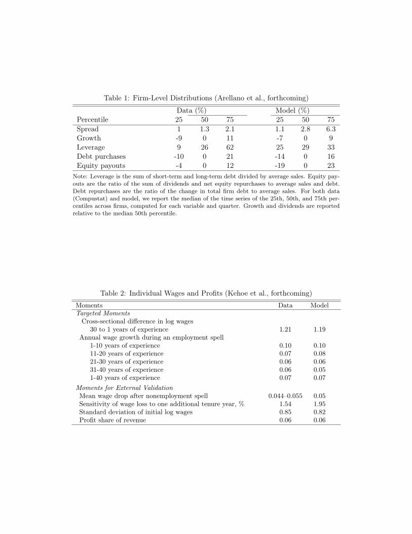
Table 1: Firm-Level Distributions (Arellano et al., forthcoming)

Data (%) Model (%)Percentile 25 50 75 25 50 75Spread 1 1.3 2.1 1.1 2.8 6.3Growth -9 0 11 -7 0 9Leverage 9 26 62 25 29 33Debt purchases -10 0 21 -14 0 16Equity payouts -4 0 12 -19 0 23

Note: Leverage is the sum of short-term and long-term debt divided by average sales. Equity pay-outs are the ratio of the sum of dividends and net equity repurchases to average sales and debt.Debt repurchases are the ratio of the change in total firm debt to average sales. For both data(Compustat) and model, we report the median of the time series of the 25th, 50th, and 75th per-centiles across firms, computed for each variable and quarter. Growth and dividends are reportedrelative to the median 50th percentile.

Table 2: Individual Wages and Profits (Kehoe et al., forthcoming)

Moments Data ModelTargeted MomentsCross-sectional difference in log wages

30 to 1 years of experience 1.21 1.19Annual wage growth during an employment spell

1-10 years of experience 0.10 0.1011-20 years of experience 0.07 0.0821-30 years of experience 0.06 0.0631-40 years of experience 0.06 0.051-40 years of experience 0.07 0.07

Moments for External ValidationMean wage drop after nonemployment spell 0.044–0.055 0.05Sensitivity of wage loss to one additional tenure year, % 1.54 1.95Standard deviation of initial log wages 0.85 0.82Profit share of revenue 0.06 0.06

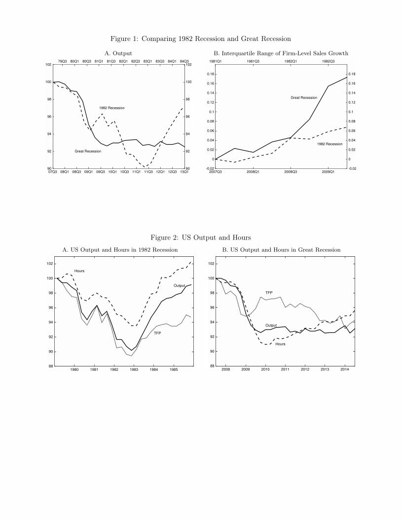
Figure 1: Comparing 1982 Recession and Great Recession

A. Output

07Q3 08Q1 08Q3 09Q1 09Q3 10Q1 10Q3 11Q1 11Q3 12Q1 12Q3 13Q190

92

94

96

98

100

10279Q3 80Q1 80Q3 81Q1 81Q3 82Q1 82Q3 83Q1 83Q3 84Q1 84Q3

90

92

94

96

98

100

102

1982 Recession

Great Recession

B. Interquartile Range of Firm-Level Sales Growth

2007Q3 2008Q1 2008Q3 2009Q1-0.02

0

0.02

0.04

0.06

0.08

0.1

0.12

0.14

0.16

0.18

1981Q1 1981Q3 1982Q1 1982Q3

-0.02

0

0.02

0.04

0.06

0.08

0.1

0.12

0.14

0.16

0.18

1982 Recession

Great Recession

Figure 2: US Output and Hours

A. US Output and Hours in 1982 Recession

1980 1981 1982 1983 1984 198588

90

92

94

96

98

100

102

Output

TFP

Hours

B. US Output and Hours in Great Recession

2008 2009 2010 2011 2012 2013 201488

90

92

94

96

98

100

102

Output

TFP

Hours

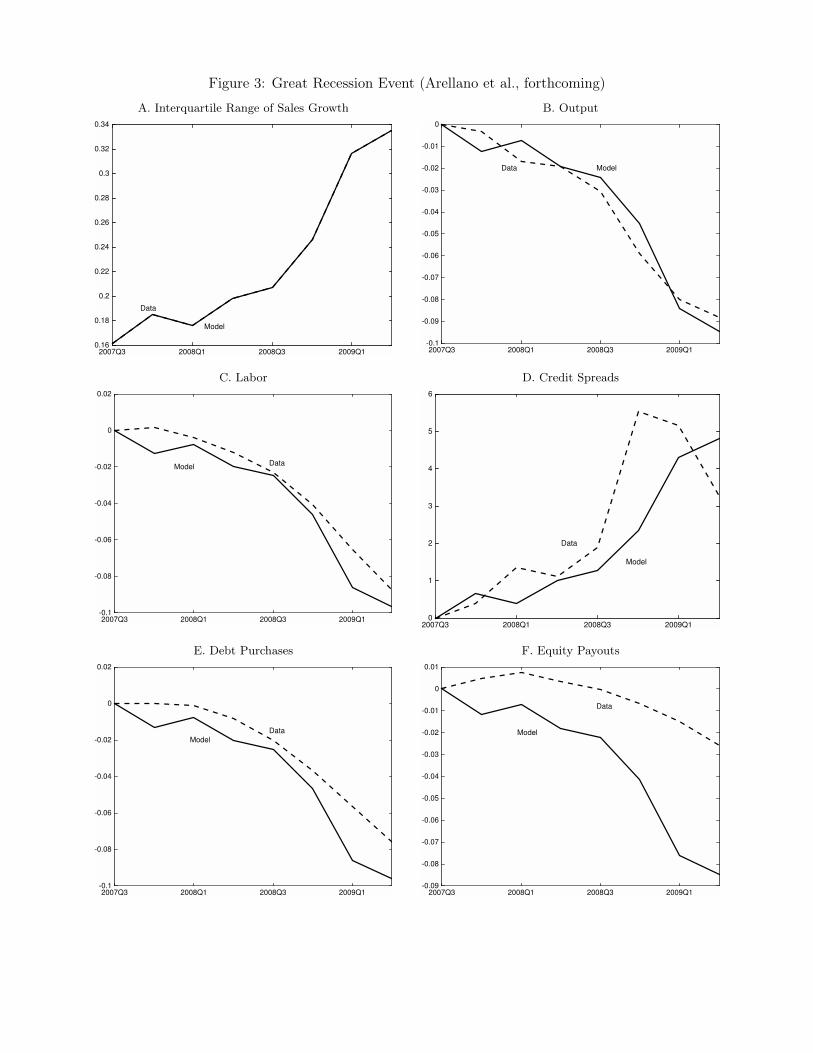
Figure 3: Great Recession Event (Arellano et al., forthcoming)

A. Interquartile Range of Sales Growth

2007Q3 2008Q1 2008Q3 2009Q10.16

0.18

0.2

0.22

0.24

0.26

0.28

0.3

0.32

0.34

Model

Data

B. Output

2007Q3 2008Q1 2008Q3 2009Q1-0.1

-0.09

-0.08

-0.07

-0.06

-0.05

-0.04

-0.03

-0.02

-0.01

0

ModelData

C. Labor

2007Q3 2008Q1 2008Q3 2009Q1-0.1

-0.08

-0.06

-0.04

-0.02

0

0.02

ModelData

D. Credit Spreads

2007Q3 2008Q1 2008Q3 2009Q10

1

2

3

4

5

6

Model

Data

E. Debt Purchases

2007Q3 2008Q1 2008Q3 2009Q1-0.1

-0.08

-0.06

-0.04

-0.02

0

0.02

Model

Data

F. Equity Payouts

2007Q3 2008Q1 2008Q3 2009Q1-0.09

-0.08

-0.07

-0.06

-0.05

-0.04

-0.03

-0.02

-0.01

0

0.01

Model

Data

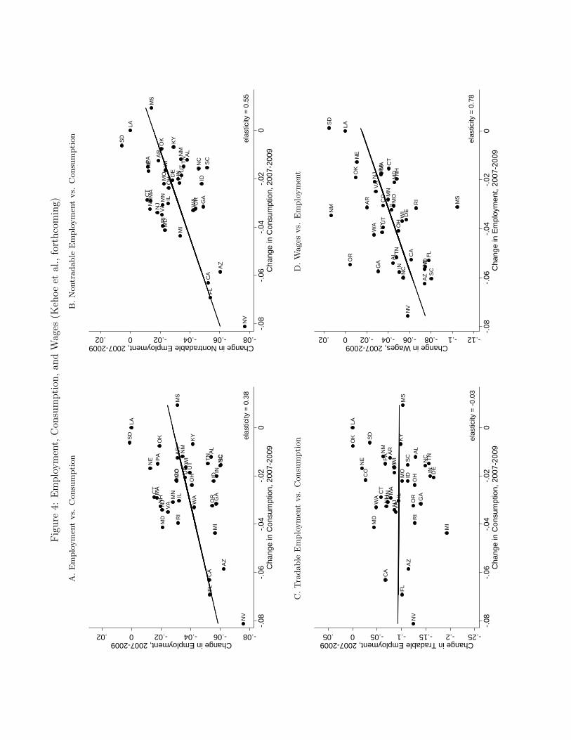
Figure4:

Employ

ment,Con

sumption,

andWag

es(K

ehoe

etal.,forthc

oming)

A.E

mploymentvs.Con

sumption

AL

AZ

AR

CA

CO

CT

DE

FL

GA

ID

IL

IN

KY

LA

MD

MA

MI

MN

MS

MO

NE

NV

NH

NJ

NM

NC

OH

OK

OR

PA

RI

SC

SD

TN

UT

VA W

A

WI

elas

ticity

= 0

.38

-.08-.06-.04-.020.02Change in Employment, 2007-2009

-.08

-.06

-.04

-.02

0C

hang

e in

Con

sum

ptio

n, 2

007-

2009

B.N

ontrad

able

Employmentvs.Con

sumption

AL

AZ

AR

CA

CO

CT

DE

FL

GA

ID

IL

INK

Y

LA

MD

MA

MI

MN

MS

MO

NE

NV

NH

NJ

NM

NC

OH

OK

OR

PA

RI

SC

SD

TN

UT

VA W

A

WI

elas

ticity

= 0

.55

-.08-.06-.04-.020.02Change in Nontradable Employment, 2007-2009

-.08

-.06

-.04

-.02

0C

hang

e in

Con

sum

ptio

n, 2

007-

2009

C.T

rada

bleEmploy

mentvs.Con

sumption

AL

AZ

AR

CA

CO

CT

DE

FL

GA

ID

IL

IN

KY

LA

MD

MA

MI

MN

MS

MO

NE

NV

NH

NJ

NM

NC

OH

OK

OR

PA

RI

SC

SD

TN

UT

VAW

A

WI

elas

ticity

= -

0.03

-.25-.2-.15-.1-.050.05Change in Tradable Employment, 2007-2009

-.08

-.06

-.04

-.02

0C

hang

e in

Con

sum

ptio

n, 2

007-

2009

D.W

ages

vs.Employ

ment

AL

AZ

AR

CA

CO

CT

DE

FL

GA ID

ILIN

KY

LA

MD

MA

MI

MN

MS

MO

NE

NV

NH

NJ

NM

NC

OH

OK

OR

PA

RI

SC

SD

TN

UT

VA

WA

WI

elas

ticity

= 0

.78

-.12-.1-.08-.06-.04-.020.02Change in Wages, 2007-2009

-.08

-.06

-.04

-.02

0C

hang

e in

Em

ploy

men

t, 20

07-2

009