Evolution of Entanglement of Two Qubits Interacting

through Local and Collective Environments

M. Merkli∗ G.P. Berman† F. Borgonovi‡ K. Gebresellasie∗

December 10, 2010

Abstract

We analyze the dynamics of entanglement between two qubits which interactthrough collective and local environments. Our approach is based on a resonancetheory which assumes a small interaction between qubits and environments andwhich gives rigorous perturbation theory results, valid for all times. We obtainexpressions for (i) characteristic time-scales for decoherence, relaxation, disentan-glement, and for (ii) the evolution of observables, valid uniformly in time t ≥ 0. Weintroduce a classification of decoherence times based on clustering of the reduceddensity matrix elements, persisting on all time-scales. We examine characteristicdynamical properties such as creation, death and revival of entanglement. We dis-cuss possible applications of our results for superconducting quantum computationand quantum measurement technologies.

1 Introduction

Entanglement plays a very important role in quantum information processes [1–7] (seealso references therein). Even if different parts of the quantum system (quantum regis-ter) are initially disentangled, entanglement naturally appears in the process of quan-tum protocols. This “constructive entanglement” must be preserved during the timeof quantum information processing. On the other hand, the system generally becomesentangled with the environment. This “destructive entanglement” must be minimizedin order to achieve a needed fidelity of quantum algorithms. The importance of theseeffects calls for the development of rigorous mathematical tools for analyzing the dy-namics of entanglement and for controlling the processes of constructive and destruc-tive entanglement. Another problem which is closely related to quantum informationis quantum measurement. Usually, for a qubit (quantum two-level system), quantummeasurements operate under the condition ~ω >> kBT , where T is the temperature,

∗Department of Mathematics and Statistics, Memorial University of Newfoundland, St. John’s,Newfoundland, Canada A1C 5S7. Email: merkli@mun.ca, http://www.math.mun.ca/merkli/

†Theoretical Division, MS B213, Los Alamos National Laboratory, Los Alamos, NM 87545, USA.Email: gpb@lanl.gov.

‡Dipartimento di Matematica e Fisica, Universita Cattolica, via Musei 41, 25121 Brescia, Italy.Email: fausto.borgonovi@unicatt.it, http://www.dmf.unicatt.it/∼borgonov and INFN, Sezione diPavia, Italy

ω is the transition frequency, ~ is the Planck constant, and kB is the Boltzmann con-stant. This condition is widely used in superconducting quantum computation, whenT ∼ 10 − 20mK and ~ω/kB ∼ 100 − 150mK. In this case, one can use Josephsonjunctions (JJ) and superconducting quantum interference devices (SQUIDs), both asqubits [8–12] and as spectrometers [13] measuring a spectrum of noise and other im-portant effects induced by the interaction with the environment. Understanding thedynamical characteristics of entanglement through the environment on a large timeinterval will help to develop new technologies for measurements not only of spectralproperties, but also of quantum correlations induced by the environment.

In this work, we describe the dynamics of the simplest quantum register of two notdirectly interacting qubits (effective spins), which interact with local and collective en-vironments. We introduce a classification of decoherence times based on the partitionof the density matrix elements, in the energy basis, into clusters which evolve indepen-dently for all times. This classification, valid for general N -level systems coupled toreservoirs, is important for dealing with quantum algorithms with large registers, wheredifferent orders of “quantumness” decay on different time scales. Given a quantum al-gorithm, the cluster classification will help to separate environment-induced effectswhich are important for its performance from those which are not.

Our strategy to describe dynamics of entanglement is based on a rigorous resonanceperturbation theory which is valid for small (fixed size) couplings and arbitrary timest ≥ 0. Previous approaches are based on a weak coupling limit (van Hove limit, Masterequation approximations, Bloch-Redfield theory) [14–18]. Two shortcomings of theseare that (a) the theory is valid only for times up to t ∼ κ

−2, where κ measures theinteraction strength between system and environment, and that (b) error terms inthe 2nd order perturbation theory approximations are not controllable (instead, byphysical arguments, errors are declared to be qualitatively small). A proof that theweak coupling limits give the correct dynamics for times smaller than t ∼ κ

−2 has beengiven in [19] (see also the books [20,21]). That the non-controlled approximations canlead to different, inequivalent expressions for the dynamics has been first shown in [22].In order to correct these two problems we have developed a rigorous description ofthe dynamics (of general finite systems coupled to reservoirs) in [23–26]. We explainhow our results eliminate problems (a) and (b) in the discussion after (3.11) below. Itis important to have a rigorous perturbation theory of dynamics, valid for all times,since (i) for not exactly solvable models one can only use a perturbative approach toestimate the characteristic dynamical parameters, and (ii) the characteristic times insystems with two and more qubits involve hugely different time-scales, ranging fromfast decay of entanglement and certain reduced density matrix elements (decoherence)to large relaxation times.

Organization of the paper. We define in Section 2 the model of two qubits interact-ing with local and collective reservoirs, via both energy-conserving and energy-exchangechannels. We present our main results on the reduced dynamics, decoherence and ther-malization rates and consequences for the dynamics of entanglement. In Section 3 wepresent the rigorous form of the reduced dynamics (equation (3.9)) and we discuss theclustering of matrix elements. In Section 4 we give the explicit resonance data of the

2

system. We compare the resonance approximation of the dynamics to the exact one foran explicitly solvable model in Section 5. Section 6 contains our main analytical resultson disentanglement, the bounds on entanglement survival and death times (equations(6.9) and (6.8)). Section 7 is devoted to a discussion of entanglement creation and itsdescription within the resonance approximation, and in Section 8 we show entanglementcreation, death and revival for the non-solvable model numerically.

2 Model and Main Results

We consider two qubits S1 and S2, each one coupled to a local reservoir, and bothtogether coupled to a collective reservoir. The Hamiltonian of the two qubits is

HS = −~ω1Sz1 − ~ω2S

z2 , (2.1)

where ω1, ω2 are the transition frequencies and Szj is the spin operator of qubit j, given

by

Sz =1

2

[1 00 −1

],

acting on spin j. The eigenvalues of HS are

E1 = −~

2(ω1 + ω2), E2 = −~

2(ω1 − ω2), E3 = −E2, E4 = −E1, (2.2)

with corresponding eigenstates

Φ1 = | + +〉, Φ2 = | + −〉, Φ3 = | − +〉, Φ4 = | − −〉, (2.3)

where the single spin energy eigenstates are |+〉 = [1 0]T , |−〉 = [0 1]T and | + +〉 =|+〉 ⊗ |+〉, etc.

Each of the three reservoirs consists of free thermal bosons at temperature T =1/β > 0, 1 with Hamiltonian

HRj=

∑

k

~ωka†j,kaj,k, j = 1, 2, 3. (2.4)

The index 3 labels the collective reservoir. The creation and annihilation operatorssatisfy [aj,k, a

†j′,k′ ] = δj,j′δk,k′. The interaction between each qubit and each reservoir

has an energy conserving and an energy exchange part. The total Hamiltonian is

H = HS +HR1 +HR2 +HR3 (2.5)

+ (λ1Sx1 + λ2S

x2 ) ⊗ φ3(g) (2.6)

+ (κ1Sz1 + κ2S

z2) ⊗ φ3(f) (2.7)

+µ1Sx1 ⊗ φ1(g) + µ2S

x2 ⊗ φ2(g) (2.8)

+ ν1Sz1 ⊗ φ1(f) + ν2S

z2 ⊗ φ2(f). (2.9)

1Our goal is to study the effect on relaxation, dephasing and evolution of entanglement comingfrom the different types of interaction (local/collective, energy-conserving/energy-exchange). We thusconsider all reservoirs at the same temperature. The results of this paper can be presented also forreservoirs at different temperatures.

3

Here,

φj(g) =1√2(a†j(g) + aj(g)), (2.10)

witha†j(g) =

∑

k

gka†j,k, aj(g) =

∑

k

g∗kaj,k. (2.11)

Also, Sxj is the spin-flip operator

Sx =1

2

[0 11 0

],

acting on qubit j. The coupling constants determine the overall (energy independent)strength of the interactions as follows:

κ1,2 energy conserving collective (spin 1, 2)λ1,2 energy exchange collectiveµ1,2 energy exchange localν1,2 energy conserving local

In the continuous mode limit, gk becomes a function g(k), k ∈ R3. Our approach is

based on analytic spectral deformation methods [23–26] and requires some analyticityof the form factors f, g. Instead of presenting this condition we will work here withexamples satisfying the condition.

(A) Let r ≥ 0, Σ ∈ S2 be the spherical coordinates of R3. The form factors h = f, g

(see (2.6)-(2.9)) are h(r,Σ) = rpe−rm

h1(Σ), with p = −1/2 + n, n = 0, 1, . . . andm = 1, 2. Here, h1 is any angular function.

This family contains the usual physical form factors [29]. We point out that we includean ultraviolet cutoff in the interaction in order for the model to be well defined. (Theminimal mathematical condition for this is that f(k), g(k) be square integrable overk ∈ R

3.)Dimensionless variables. In the rest of the paper we use dimensionless functions

and parameters. For this we introduce a characteristic frequency ω0 (to be defined laterin Section 8) and the dimensionless energies, temperature, frequencies, wave vectors ofthermal excitations and time, by setting

E′n = En/(~ω0), f ′k = fk/(~ω0), g′k = gk/(~ω0), T ′ = kBT/(~ω0),

β′ = 1/T ′, ω′k = ωk/ω0, ~k′ = c~k/ω0, t′ = ω0t,

where c is the speed of light. In all that follows we now omit the index “prime”.

Main results

• We introduce for the first time a model which includes simultaneously interactionsof two non-interacting spins (qubits) with local and collective, energy conserving andenergy-exchange environments. We develop a resonant perturbation theory allowing

4

us to rigorously (deriving conditions of applicability) (i) calculate the renormalizationof thermalization and decoherence rates and (ii) calculate the dynamics of creation ofentanglement due to the competition of destructive effects of local environments andconstructive effects of collective environments.

• Evolution of reduced denisty matrix. We derive an expression for the reduced den-sity matrix of the two qubits (3.9) (reservoirs traced out). We identify a dominant partof the dynamics and a remainder term. The dominant part is the effective dynamicsinduced by the interaction with the reservoirs. The remainder is small, homogeneouslyin time t ≥ 0. Matrix elements (in the energy basis (2.3)) belonging to the same energydifference form a ‘cluster’ evolving as a group in a correlated way. Elements from differ-ent clusters evolve independently. Within each cluster, the dynamics is markovian: itis obtained from the initial matrix elements via time-dependent transition amplitudes.The latter are characterized by (superpositions of) functions eitε, with ε ∈ C. In thisway, each cluster has its own (minimal) decoherence rate, determined by the imaginaryparts of the ε. The rate for the cluster containing the diagonal is the thermalizationrate (relaxation to equilibrium). These rates measure how long a given cluster survives(or is out of equilibrium). Depending on the interaction parameters, the rates varyconsiderably between different clusters.

Within the framework of the Bloch-Redfield and master equation theory, the clus-tering is called the rotating wave, or secular approximation. It is heuristically arguedto hold for times up to order κ

−2 (small coupling constants κ) [14–18, 21, 34]. Ourapproach shows rigorously that the clustering holds for all times t ≥ 0.

For purely energy conserving interactions, this model can be solved explicitly (seeSection 5). In this situation, each matrix element evolves independently, [ρt]mn =eiS(t)e−Γ(t)[ρ0]mn for some real functions Γ(t) ≥ 0 and S(t). In the limit of large times,both S(t) and Γ(t) become linear in t and then eiS(t)e−Γ(t) becomes eitε, with ourexpressions for ε. Our method shows that the true dynamics can be expressed, up toan error term, by the ‘asymptotic’ quantities ε for all times. Of course, for the notexplicitly solvable model (energy exchange interactions), it is impossible to know theanalogue of the functions S(t) and Γ(t). Nevertheless, the quantities ε still exist, and wecan calculate them and express the true dynamics via them. This gives a representationof the true dynamics correct up to an error which is small, homogeneously in time t ≥ 0.

• Relaxation and cluster decoherence rates. We calculate the cluster decoherenceand termalization rates for the qubits in presence of all couplings (2.6)-(2.9). Wepresent here the formulas for two clusters: the diagonal, γth, and the one associated tothe energy difference −ω1, γ

dec2 (matrix elements (1, 3) and (2, 4), see equations (2.2)

[in units with ~ = 1]). The complete list of rates is given in (4.11)-(4.15). The spectraldensity of a reservoir is

Jh(ω) =π

4ω2

∫

S2

|h(ω,Σ)|2dΣ. 2

2Let Ch(t) = 12[〈φ(h)eitHRφ(h)e−itHR〉β + 〈eitHRφ(h)e−itHRφ(h)〉β] be the symmetrized correlation

function of a reservoir in thermal equilibrium at temperature T = 1/β, with HR and φ(h) given in (2.4)

and (2.10). The Fourier transform bCh(ω) =R ∞

0e−iωtC(t)dt, ω ≥ 0, is related to the spectral density

5

Here, h = h(ω,Σ) is a form factor, a square integrable function of k = (r,Σ) ∈ R3

(ω ≥ 0, Σ ∈ S2; spherical coordinates). Set for ω > 0 (see also (2.12))

σh(ω) = Jh(ω) coth(βω/2) and σh(0) = limω→0

σh(ω) =2

βlimω→0

Jh(ω)

ω.

The relaxation rate is given by

γth = minj=1,2

{(λ2

j + µ2j)σg(ωj)

}+O(κ4).

It involves the reservoir spectral density at the frequencies of the qubits only. Thisrate vanishes in absence of energy-exchange couplings (no thermalization without en-ergy exchange). The expression coincides with that obtained from the Bloch-Redfieldtheory [8,21] for two qubits exchanging energy with local and collective reservoirs. Thedecoherence rate of the above-mentioned cluster is

γdec2 = 1

2 (λ21 + µ2

1)σg(ω1) + 12(λ2

2 + µ22)σg(ω2) + (κ2

1 + ν21)σf (0) − Y2 +O(κ4).

Here,

Y2 =∣∣∣ℑ

[4κ2

1κ22r

2 − 14(λ2

2 + µ22)

2σ2g(ω2) − 4iπ−1κ1κ2r (λ2

2 + µ22)Jg(ω2)

]1/2∣∣∣,

with r = P.V.∫

R3|f |2|k| d3k. The rate γdec

2 has a contribution in which the reservoirs

contribute in an uncorrelated way by adding single terms (the first three terms onr.h.s.). The decay is driven by energy-exchange processes of the local and collectivereservoirs (playing the same role), plus the energy-conserving (“scattering”) processes,involving the spectral density at frequency zero. The reservoirs play a symmetrical rolein these contributions (coupling constant square times σ at the appropriate frequency).However, the term −Y2 is a complicated function of the parameters of energy-conservingand exchange collective and energy-exchange local reservoirs. This function does notonly involve the spectral density at the frequencies of the qubits, but also the quantityr, which is associated with the Lamb shift induced by the energy-conserving collectiveinteraction. (Real part of the complex effective energies.)

If at least one of the qubits is not coupled via the energy conserving collectiveinteraction (κ1κ2 = 0), then Y2 = 1

2(λ22 + µ2

2)σg(ω2) and consequently the term −Y2 inthe expression for γdec

2 compensates the decay induced by the energy exchange processesat frequency ω2. In this case, the decoherence rate for this cluster does not depend onω2. The same rate is obtained if qubit 2 is not coupled via energy exchange interactions,or if the spectral density at ω2 vanishes (then we have Y2 = 0).

We are not aware of any work giving the decoherence rates for this or similar modelswith all interactions, even by using the Bloch-Redfield approximation.

• Dynamics of entanglement. Using the expression for the evolution of the re-duced density matrix via cluster decoherence and relaxation times, and phases, we cancalculate the dynamics of the concurrence of the two qubits.

byRe bCh(ω) = Jh(ω) coth(βω/2). (2.12)

6

In Section 6 we consider the process of disentanglement due to the interaction withthe environments. The whole system relaxes to equilibrium driven by energy exchangeprocesses.3 The reduced state of the two qubits is then just the equilibrium staterelative to the energy (2.1), modulo a correction of order κ

2. It is easy to see thatany state in a neighbourhood of the equilibrium state of two qubits has concurrencezero. The size of this neighbourhood depends on the temperature. It follows that forfixed temperature and κ

2 small enough, the qubits, driven into the neighbourhoodof the equilibrium state, will eventually become disentangled, no matter what initialstate they were in. In (6.8) and (6.9) we give bounds on the entanglement survivaltime (concurrence strictly positive before this time is reached, for given initial state)and entanglement death time (concurrence zero for all times after this instant). Thisanalysis is purely analytical. To obtain the entanglement death time, which may bevery large, it is important that we know rigorous estimates on the true dynamics for alltimes, even t→ ∞. This information is available in our approach, as our perturbationtheory is valid homogeneously in time.

In Sections 7 and 8 we study the opposite process, that of creation of entanglementby interaction with reservoirs. It is known that initially unentangled qubits can becomeentangled by interaction with a collective reservoir. In [39] an explicitly solvable modelwith energy conserving collective interaction is considered. It is shown in [39] thatan initially unentangled initial state (7.1) acquires entanglement and undergoes deathand revival of entanglement. We analyze the evolution of concurrence in our resonanceapproximation numerically, in presence of the full interaction (2.6)-(2.9). We find thatif the strength of the local couplings are stronger than the collective one, then noconcurrence is created. In the opposite case, concurrence is created, dies out and getsrevived, similarly to the explicitly solvable model. This shows that even though ourresonance approximation is a ‘markovian approximation’, it captures essential featuresin the study of entanglement.

3 Evolution of qubits: resonance approximation

We take initial states where the qubits are not entangled with the reservoirs. Let ρS

be an arbitrary initial state of the qubits, and let ρRjbe the thermal equilibrium state

of reservoir Rj. Let ρS(t) be the reduced density matrix of the two qubits at time t.The reduced density matrix elements in the energy basis are

[ρS(t)]mn := 〈Φm, ρS(t)Φn〉= TrR1+R2+R3

[ρS ⊗ ρR1 ⊗ ρR2 ⊗ ρR3 e−itH |Φn〉〈Φm| eitH

], (3.1)

where we take the trace over all reservoir degrees of freedom. Under the non-interactingdynamics (all coupling parameters zero), we have

[ρ(t)]mn = eitemn [ρ(0)]mn, (3.2)

3If the reservoirs are not all at the same temperature, then the final state of the whole system is a‘Non-Equilibrium Steady State’. Our approach gives the dynamics of the qubits also in this situation,see [28].

7

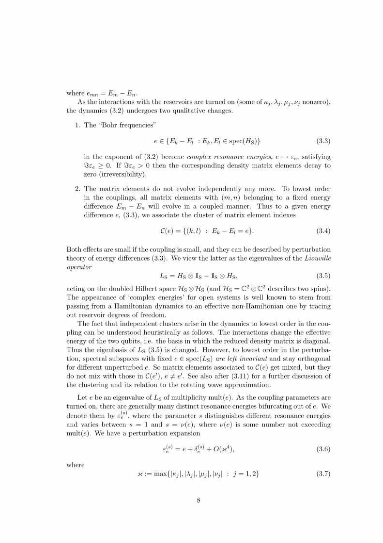
where emn = Em −En.As the interactions with the reservoirs are turned on (some of κj , λj , µj , νj nonzero),

the dynamics (3.2) undergoes two qualitative changes.

1. The “Bohr frequencies”

e ∈ {Ek − El : Ek, El ∈ spec(HS)} (3.3)

in the exponent of (3.2) become complex resonance energies, e 7→ εe, satisfyingℑεe ≥ 0. If ℑεe > 0 then the corresponding density matrix elements decay tozero (irreversibility).

2. The matrix elements do not evolve independently any more. To lowest orderin the couplings, all matrix elements with (m,n) belonging to a fixed energydifference Em − En will evolve in a coupled manner. Thus to a given energydifference e, (3.3), we associate the cluster of matrix element indexes

C(e) = {(k, l) : Ek − El = e}. (3.4)

Both effects are small if the coupling is small, and they can be described by perturbationtheory of energy differences (3.3). We view the latter as the eigenvalues of the Liouvilleoperator

LS = HS ⊗ 1lS − 1lS ⊗HS, (3.5)

acting on the doubled Hilbert space HS ⊗HS (and HS = C2 ⊗C

2 describes two spins).The appearance of ‘complex energies’ for open systems is well known to stem frompassing from a Hamiltonian dynamics to an effective non-Hamiltonian one by tracingout reservoir degrees of freedom.

The fact that independent clusters arise in the dynamics to lowest order in the cou-pling can be understood heuristically as follows. The interactions change the effectiveenergy of the two qubits, i.e. the basis in which the reduced density matrix is diagonal.Thus the eigenbasis of LS (3.5) is changed. However, to lowest order in the perturba-tion, spectral subspaces with fixed e ∈ spec(LS) are left invariant and stay orthogonalfor different unperturbed e. So matrix elements associated to C(e) get mixed, but theydo not mix with those in C(e′), e 6= e′. See also after (3.11) for a further discussion ofthe clustering and its relation to the rotating wave approximation.

Let e be an eigenvalue of LS of multiplicity mult(e). As the coupling parameters areturned on, there are generally many distinct resonance energies bifurcating out of e. We

denote them by ε(s)e , where the parameter s distinguishes different resonance energies

and varies between s = 1 and s = ν(e), where ν(e) is some number not exceedingmult(e). We have a perturbation expansion

ε(s)e = e+ δ(s)e +O(κ4), (3.6)

whereκ := max{|κj |, |λj |, |µj |, |νj | : j = 1, 2} (3.7)

8

and where δ(s)e = O(κ2) and ℑδ(s)e ≥ 0. The lowest order corrections δ

(s)e are the

eigenvalues of an explicit level shift operator Λe (see [23–26]), acting on the eigenspace

of LS associated to e. There are two bases {η(s)e } and {η(s)

e } of the eigenspace, satisfying

Λeη(s)e = δ(s)e η(s)

e , [Λe]∗η(s)

e = δ(s)e∗η(s)

e ,⟨η(s)

e , η(s′)e

⟩= δs,s′ . (3.8)

We call the eigenvectors η(s)e and η

(s)e the ‘resonance vectors’. We take interaction pa-

rameters (f, g and the coupling constants) such that the following condition is satisfied.

(F) There is complete splitting of resonances under perturbation at second order, i.e.,

all the δ(s)e are distinct for fixed e and varying s.

This condition implies in particular that there are mult(e) distinct resonance energies

ε(s)e , s = 1, . . . ,mult(e) bifurcating out of e, so that in the above notation, ν(e) =

mult(e). Explicit evaluation of δ(s)e shows that condition (F) is satisfied for generic

values of the interaction parameters (see also (4.11)-(4.15)).

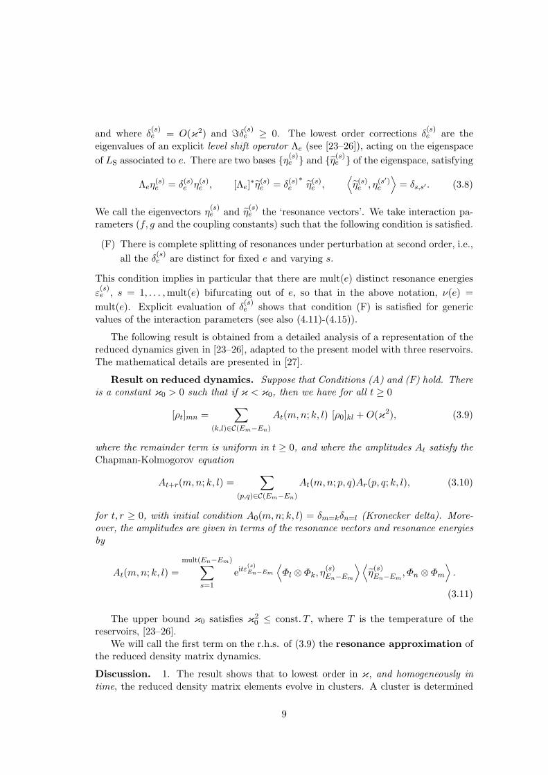
The following result is obtained from a detailed analysis of a representation of thereduced dynamics given in [23–26], adapted to the present model with three reservoirs.The mathematical details are presented in [27].

Result on reduced dynamics. Suppose that Conditions (A) and (F) hold. Thereis a constant κ0 > 0 such that if κ < κ0, then we have for all t ≥ 0

[ρt]mn =∑

(k,l)∈C(Em−En)

At(m,n; k, l) [ρ0]kl +O(κ2), (3.9)

where the remainder term is uniform in t ≥ 0, and where the amplitudes At satisfy theChapman-Kolmogorov equation

At+r(m,n; k, l) =∑

(p,q)∈C(Em−En)

At(m,n; p, q)Ar(p, q; k, l), (3.10)

for t, r ≥ 0, with initial condition A0(m,n; k, l) = δm=kδn=l (Kronecker delta). More-over, the amplitudes are given in terms of the resonance vectors and resonance energiesby

At(m,n; k, l) =

mult(En−Em)∑

s=1

eitε(s)En−Em

⟨Φl ⊗ Φk, η

(s)En−Em

⟩⟨η

(s)En−Em

, Φn ⊗ Φm

⟩.

(3.11)

The upper bound κ0 satisfies κ20 ≤ const. T , where T is the temperature of the

reservoirs, [23–26].We will call the first term on the r.h.s. of (3.9) the resonance approximation of

the reduced density matrix dynamics.

Discussion. 1. The result shows that to lowest order in κ, and homogeneously intime, the reduced density matrix elements evolve in clusters. A cluster is determined

9

by indices in a fixed C(e). Within each cluster the dynamics has the structure of aMarkov process. Moreover, the transition amplitudes of this process are given by theresonance data. They can be calculated explicitly in concrete models.

2. The transision amplitudes (3.11) depend on all orders in the coupling κ, since

the ε(s)e do, see (3.6). The inclusion of all orders in At allows us to obtain a remainder

term O(κ2) in (3.9) which is bounded uniformly in t ≥ 0. This is one advantage ofour approach over the usual weak coupling methods (see introduction and referencesmentioned there). Simply neglecting terms of order higher than two in the exponents

ε(s)e yields wrong predictions as can be easily seen: In degenerate systems it happens

frequently that second order contributions δ(s)e to ε

(s)e vanish, and hence one would

classify all states in the subspace defined by e wrongly as being invariant states (nodecay), while in reality those states are decaying on a time-scale t ∼ κ

−4 (or slower).Our result captures decay at any order (rate), while the usual methods can only describedecay happening on a time scale t ∼ κ

−2.3. Cluster classification of density matrix elements. The main dynamics partitions

the reduced dynamics into independent clusters of jointly evolving matrix elements,according to (3.4). In the usual weak-coupling limit method, clustering of matrixelements is obtained by the so-called rotating wave (secular) approximation. However,since that method is only accurate up to times at most t ∼ κ

−2, the clustering is alsoguaranteed only up to that scale. Our result proves that such a clustering holds on alltime-scales.

Each cluster has its associated decay rate. It is possible that some clusters decayvery quickly, while some others stay populated for much longer times. The resonancedynamics shows which parts of the matrix elements disappear when, revealing a patternof where in the density matrix quantum properties are lost at which time. The samefeature holds for an arbitrary N -level system coupled to reservoirs, [23–26], and notablyfor complex systems (N >> 1). In particular, this approach may prove useful in theanalysis of feasibility of quantum algorithms performed on N -qubit registers. We pointout that that the diagonal belongs always to a single cluster, namely the one associatedwith e = 0. If the energies of the N -level system are degenerate, then some off-diagonalmatrix elements belong to the same cluster as the diagonal as well.

4. The sum in (3.9) alone, which is the main term in the expansion, preservesthe hermiticity but not the positivity of density matrices. In other words, the matrixobtained from this sum may have negative eigenvalues. Since by adding O(κ2) we doget a true density matrix, the mentioned negativity of eigenvalues can only be of O(κ2).This can cause complications if one tries to calculate for instance the concurrence byusing the main term in (3.9) alone. Indeed, concurrence is not defined in general for a‘density matrix’ having negative eigenvalues. See also section 8.

5. It is well known that the time decay of matrix elements is not exponentialfor all times. For example, for small times it is quadratic in t [29]. How is thisbehaviour compatible with the representation (3.9), (3.11), where only exponentialtime factors eitε are present? The answer is that up to an error term of O(κ2), the“overlap coefficients” (scalar products in (3.11)) mix the exponentials in such a way asto produce the correct time behaviour.

10

6. Since the coupled system has an equilibrium state, one of the resonances ε(s)0 is

always zero [30], we set ε(1)0 = 0. The condition ℑε(s)e > 0 for all e, s except e = 0, s = 1

is equivalent to the entire system (qubits plus reservoirs) converging to its equilibriumstate for large times.

As mentioned, decay of matrix elements is not in general exponential, but we cannevertheless represent it (approximate to order κ

2) in terms of superpositions of ex-ponentials, for all times t ≥ 0. In regimes where the actual dynamics has exponentialdecay, the rates coincide with those we obtain from the resonance theory (large timedynamics, see Section 5 and also [23–26, 29]). It is therefore reasonable to define thethermalization rate by

γth = mins≥2

ℑε(s)0 ≥ 0

and the cluster decoherence rate associated to C(e), e 6= 0, by

γdece = min

1≤s≤mult(e)ℑε(s)e ≥ 0.

The interpretation is that the cluster of matrix elements of the true density matrixassociated to e 6= 0 decays to zero, modulo an error term O(κ2), at the rate γdec

e , andthe cluster containing the diagonal approaches its equilibrium (Gibbs) value, moduloan error term O(κ2), at rate γth. If γ is any of the above rates, then τ = 1/γ is thecorresponding (thermalization, decoherence) time.

Remark on the markovian property. In the first point discussed after (3.11),we remark that within a cluster, our approximate dynamics of matrix elements hasthe form of a Markov process. In the theory of markovian master equations, one con-structs commonly an approximate dynamics given by a markovian quantum dynamicalsemigroup, generated by a so-called Lindblad (or weak coupling) generator [21]. Ourrepresentation is not in Lindblad form (indeed, it is not even a positive map on densitymatrices). To make the meaning of the markovian property of our dynamics clear,we consider a fixed cluster C and denote the associated pairs of indices by (mk, nk),k = 1, . . . ,K. Retaining only the main part in (3.9), and making use of (3.10) weobtain for t, s ≥ 0

[ρt+s]m1n1

...[ρt+s]mKnK

= AC(t)

[ρs]m1n1

...[ρs]mKnK

, (3.12)

where [AC(t)]mjnj ,mlnl= At(mj , nj;ml, nl), c.f. (3.11). Thus the dynamics of the

vector having as components the density matrix elements, has the semi-group propertyin the time variable, with generator GC := d

dtAC(0),

[ρt]m1n1

...[ρt]mKnK

= etGC

[ρ0]m1n1

...[ρ0]mKnK

. (3.13)

This is the meaning of the Markov property of the resonance dynamics.

11

While the fact that our resonance approximation is not in the form of the weakcoupling limit (Lindblad) may represent disadvantages in certain applications, it mayalso allow for a description of effects possibly not visible in a markovian master equa-tion approach. Based on results [1–4,31], one may believe that revival of entanglementis a non-markovian effect, in the sense that it is not detectable under the markovianmaster equation dynamics (however, we are not aware of any demonstration of thisresult). Nevertheless, as we show in our numerical analysis below, the resonance ap-proximation captures this effect (see Figure 1). We may attempt to explain this asfollows. Each cluster is a (indpendent) markov process with its own decay rate, andwhile some clusters may depopulate very quickly, the ones responsible for creatingrevival of entanglement may stay alive for much longer times, hence enabling that pro-cess. Clearly, on time-scales larger than the biggest decoherence time of all clusters, thematrix is (approximately) diagonal, and typically no revival of entanglement is possibleany more.

4 Explicit resonance data

We consider the Hamiltonian HS, (2.4), with parameters 0 < ω1 < ω2 s.t. ω2/ω1 6= 2.This assumption is a non-degeneracy condition which is not essential for the applica-bility of our method (but lightens the exposition). The eigenvalues of HS are given by(2.2) and the spectrum of LS is {e1,±e2,±e3,±e4,±e5}, with non-negative eigenvalues

e1 = 0, e2 = −ω1, e3 = −ω2, e4 = −(ω2 − ω1), e5 = −(ω1 + ω2), (4.1)

having multiplicities m1 = 4, m2 = m3 = 2, m4 = m5 = 1, respectively. According to(4.1), the grouping of jointly evolving elements of the density matrix above and on thediagonal is given by4

C1 := C(e1) = {(1, 1), (2, 2), (3, 3), (4, 4)} (4.2)

C2 := C(e2) = {(1, 3), (2, 4)} (4.3)

C3 := C(e3) = {(1, 2), (3, 4)} (4.4)

C4 := C(−e4) = {(2, 3)} (4.5)

C5 := C(e5) = {(1, 4)} (4.6)

There are five clusters of jointly evolving elements (on and above the diagonal). Onecluster is the diagonal, represented by C1.

Recall expression (2) for the spectral density Jh(ω) of a reservoir. We define forω > 0

σh(ω) = coth(βω/2)Jh(ω), (4.7)

(see also (2.12)) and we have

σh(0) = limω→0

σh(ω) =2

βlimω→0

Jh(ω)

ω.

4Since the density matrix is hermitian, it suffices to know the evolution of the elements on andabove the diagonal.

12

Let

Y2 =∣∣∣ℑ

[4κ2

1κ22r

2 − 14(λ2

2 + µ22)

2σ2g(ω2) − 4iπ−1κ1κ2r (λ2

2 + µ22)Jg(ω2)

]1/2∣∣∣, (4.8)

Y3 =∣∣∣ℑ

[4κ2

1κ22r

2 − 14(λ2

1 + µ21)

2σ2g(ω1) − 4iπ−1κ1κ2r (λ2

1 + µ21)Jg(ω1)

]1/2∣∣∣, (4.9)

(principal value square root with branch cut on negative real axis) where

r = P.V.

∫

R3

|f |2|k| d3k. (4.10)

The following results are obtained by an explicit calculation of level shift operators.Details are presented in [27].

Result on decoherence and thermalization rates. The thermalization anddecoherence rates are given by

γth = minj=1,2

{(λ2

j + µ2j )σg(ωj)

}+O(κ4) (4.11)

γdec2 = 1

2(λ21 + µ2

1)σg(ω1) + 12 (λ2

2 + µ22)σg(ω2)

−Y2 + (κ21 + ν2

1)σf (0) +O(κ4) (4.12)

γdec3 = 1

2(λ21 + µ2

1)σg(ω1) + 12 (λ2

2 + µ22)σg(ω2)

−Y3 + (κ22 + ν2

2)σf (0) +O(κ4) (4.13)

γdec4 = (λ2

1 + µ21)σg(ω1) + (λ2

2 + µ22)σg(ω2)

+[(κ1 − κ2)

2 + ν21 + ν2

2

]σf (0) +O(κ4) (4.14)

γdec5 = (λ2

1 + µ21)σg(ω1) + (λ2

2 + µ22)σg(ω2)

+[(κ1 + κ2)

2 + ν21 + ν2

2

]σf (0) +O(κ4) (4.15)

Discussion. 1. The thermalization rate depends on energy-exchange parameters λj ,µj only. This is natural since an energy-conserving dynamics leaves the populationsconstant. If the interaction is purely energy-exchanging (κj = νj = 0), then all the ratesdepend symmetrically on the local and collective interactions, through λ2

j+µ2j . However,

for purely energy-conserving interactions (λj = µj = 0) the rates are not symmetrical inthe local and collective terms. (E.g. γdec

4 depends only on local interaction if κ1 = κ2.)The terms Y2, Y3 are complicated nonlinear combinations of exchange and conservingterms. This shows that effect of the energy exchange and conserving interactions arecorrelated.

2. We see from (4.7) that the leading orders of the rates (4.11)-(4.15) do not de-pend on an ultraviolet features of the form factors f, g. (However, σf,g(0) depends onthe infrared behaviour.) Of course, the second order expressions of the decay ratesare consistent with the usual Fermi Golden Rule of energy-conserving 2nd order pro-cesses. The coupling constants, e.g. λ2

j in (4.11) multiply σg(ωj), i.e., the rates involvequantities like (see (4.7))

π

4λ2

j

∫

R3

coth(β|k|/2

) ∣∣g(|k|,Σ)∣∣2 δ(1)(|k| − ωj) d3k. (4.16)

13

The one-dimensional Dirac delta function appears due to energy conservation of pro-cesses of order κ

2, and ωj is (one of) the Bohr frequencies of a qubit. Thus energyconservation chooses the evaluation of the form factors at finite momenta and thusan ultraviolet cutoff is not visible in these terms (due to the Fermi Golden Rule ofenergy-conserving processes). However, we do not know how to control the error termsO(κ4) in (4.11)-(4.15) homogeneously in the cutoff.

3. The case of a single qubit interacting with a thermal bose gas has been extensivelystudied, and decoherence and thermalization rates for the spin-boson system have beenfound using different techniques, [32–34]. We recover the spin-boson model by settingall our couplings in (2.5)-(2.9) to zero, except for λ1 = κ1 ≡ λ, and setting f = g. Inthis case the relaxation rate is

γth = 2λ2 coth(βω/2)J(ω),

where ω is the transition frequency of qubit (in units where ~ = 1). The decoherencerate is given by

γdec =γth

2+ 2λ2σh(0).

These rates obtained with our resonance method agree with those obtained in [32–34]by the standard Bloch-Redfield approximation.

Remark on the limitations of the resonance approximation. The dynam-ics (3.9) can only resolve the evolution of quantities larger than O(κ2). For in-stance, assume that in an initial state of the two qubits, all off-diagonal density ma-trix elements are of the order of unity (relative to κ). As time increases, the off-

diagonal matrix elements decrease, and for times t satisfying e−tγdecj ≤ O(κ2), the

off-diagonal cluster Cj is of the same size O(κ2) as the error in (3.9). Hence the evo-lution of this cluster can be followed accurately by the resonance approximation for

times t < ln(κ−2)/γdecj ∝ ln(κ−2)

κ2(1+T ), where T is the temperature. Here, T,κ (and other

parameters) are dimensionless. To describe the cluster in question for larger times,one has to push the perturbation theory to higher order in κ. It is now clear thatif a cluster is initially not populated, the resonance approximation does not give anyinformation about the evolution of this cluster, other than saying that its elements willbe O(κ2) for all times.

Below we investigate analytically decay of entanglement (section 6) and numeri-cally creation of entanglement (section 8). For the same reasons as just outlined, ananalytical study of entanglement decay is possible if the initial entanglement is largecompared to O(κ2). However, the study of creation of entanglement is more subtlefrom this point of view, since one must detect the emergence of entanglement, presum-ably of order O(κ2) only, starting from zero entanglement. We show in our numericalanalysis that entanglement of size 0.3 is created independently of the value of κ (rang-ing from 0.01 to 1). We are thus sure that the resonance approximation does detectcreation of entanglement, even if it may be of the same order of magnitude as thecouplings. Whether this is correct for other quantities than entanglement is not clear,and so far, only numerical investigations seem to be able to give an answer. As an ex-ample where things can go wrong with the resonance approximation we mention that

14

for small times, the approximate density matrix has negative eigenvalues. This makesthe notion of concurrence of the approximate density matrix ill-defined for small times.

5 Comparison between exact solution and resonance ap-

proximation: explicitly solvable model

We consider the system with Hamiltonian (2.5)-(2.11) and λ1 = λ2 = 0, µ1 = µ2 = 0,κ1 = κ2 = κ and ν1 = ν2 = ν. This energy-conserving model can be solved explicitly[23–26,29] and has the exact solution

[ρt]mn = [ρ0]mn e−it(Em−En) eiκ2amnS(t) e−[κ2bmn+ν2cmn]Γ(t) (5.1)

where

(amn) =

0 −1 −1 01 0 0 11 0 0 10 −1 −1 0

, (bmn) =

0 1 1 41 0 0 11 0 0 14 1 1 0

, (cmn) =

0 1 1 21 0 2 11 2 0 12 1 1 0

and

S(t) =1

2

∫

R3

|f(k)|2 |k|t− sin(|k|t)|k|2 d3k (5.2)

Γ(t) =

∫

R3

|f(k)|2 coth(β|k|/2)sin2(|k|t/2)|k|2 d3k. (5.3)

On the other hand, the main contribution (the sum) in (3.9) yields the resonance

approximation to the true dynamics, given by

[ρt]mm.= [ρ0]mm m = 1, 2, 3, 4 (5.4)

[ρt]1n.= e−it(E1−En) e−itκ2r/2e−t(κ2+ν2)σf (0)[ρ0]1n n = 2, 3 (5.5)

[ρt]14.= e−it(E1−E4) e−2t(2κ2+ν2)σf (0)[ρ0]14 (5.6)

[ρt]23.= e−it(E2−E3) e−2tκ2σf (0)[ρ0]23 (5.7)

[ρt]m4.= e−it(Em−E4) eitκ2r/2 e−t(κ2+ν2)σf (0)[ρ0]m4 m = 2, 3 (5.8)

The dotted equality sign.= signifies that the left side equals the right side modulo an

error term O(κ2 + ν2), homogeneously in t ≥ 0.5 Clearly the decoherence functionΓ(t) and the phase S(t) are nonlinear in t and depend on the ultraviolet behaviour off . On the other hand, our resonance theory approach yields a representation of thedynamics in terms of a superposition of exponentially decaying factors. From (5.1) and(5.4)-(5.8) we see that the resonance approximation is obtained from the exact solutionby making the replacements

S(t) 7→ 12rt, (5.9)

Γ(t) 7→ σf (0)t. (5.10)

5To arrive at (5.4)-(5.8) one calculates the At in (3.9) explicitly, to second order in κ and ν. Thedetails are given in [27].

15

We emphasize again that, according to (3.9), the difference between the exact solu-tion and the one given by the resonance approximation is of the order O(κ2 + ν2),homogeneously in time, and where O(κ2 + ν2) depends on the ultraviolet behaviour ofthe couplings. This shows in particular that up to errors of O(κ2 + ν2), the dynamicsof density matrix elements is simply given by a phase change and a possibly decay-ing exponential factor, both linear in time and entirely determined by r and σf (0).Of course, the advantage of the resonance approximation is that even for not exactlysolvable models, we can approximate the true (unknown) dynamics by an explicitlycalculable superposition of exponentials with exponents linear in time, according to(3.9). Let us finally mention that one easily sees that

limt→∞

S(t)/t = r/2 and limt→∞

Γ(t)/t = σf (0),

so (5.9) and (5.10) may indicate that the resonance approximation is closer to the truedynamics for large times – but nevertheless, our analysis proves that the two are closetogether (O(κ2 + ν2)) homogeneously in t ≥ 0.

6 Disentanglement

In this section we apply the resonance method to obtain estimates on survival anddeath of entanglement under the full dynamics (2.5)-(2.9) and for an initial state of theform ρS ⊗ ρR1 ⊗ ρR2 ⊗ ρR3, where ρS has nonzero entanglement and the reservoir initialstates are thermal, at fixed temperature T = 1/β > 0. Let ρ be the density matrix oftwo qubits 1/2. The concurrence [35, 36] is defined by

C(ρ) = max{0,√ν1 −[√ν2 +

√ν3 +

√ν4

]}, (6.1)

where ν1 ≥ ν2 ≥ ν3 ≥ ν4 ≥ 0 are the eigenvalues of the matrix

ξ(ρ) = ρ(σy ⊗ σy)ρ∗(σy ⊗ σy). (6.2)

Here, ρ∗ is obtained from ρ by representing the latter in the energy basis and then

taking the elementwise complex conjugate, and σy is the Pauli matrix σy =

[0 −ii 0

].

The concurrence is related in a monotone way to the entanglement of formation, and(6.1) takes values in the interval [0, 1]. If C(ρ) = 0 then the state ρ is separable,meaning that ρ can be written as a mixture of pure product states. If C(ρ) = 1 we callρ maximally entangled.

Let ρ0 be an initial state of S. The smallest number t0 ≥ 0 s.t. C(ρt) = 0for all t ≥ t0 is called the disentanglement time (also ‘entanglement sudden deathtime’, [1–4, 37]). If C(ρt) > 0 for all t ≥ 0 then we set t0 = ∞. The disentanglementtime depends on the initial state. Consider the family of pure initial states of S given

by

ρ0 = |ψ〉〈ψ|, with |ψ〉 =a1√

|a1|2 + |a2|2| + +〉 +

a2√|a1|2 + |a2|2

| − −〉,

16

where a1, a2 ∈ C are arbitrary (not both zero). The initial concurrence is

C(ρ0) = 2|ℜ a1a

∗2|

|a1|2 + |a2|2,

which covers all values between zero (e.g. a1 = 0) to one (e.g. a1 = a2 ∈ R). Accordingto (3.9), the density matrix of S at time t ≥ 0 is given by

ρt =

p1 0 0 α0 p2 0 00 0 p3 0α∗ 0 0 p4

+O(κ2), (6.3)

with remainder uniform in t, and where pj = pj(t) and α = α(t) are given by the

main term on the r.h.s. of (3.9). The initial conditions are p1(0) = |a1|2|a1|2+|a2|2 , p2(0) =

p3(0) = 0, p4(0) = |a2|2|a1|2+|a2|2 , and α(0) =

a∗1a2

|a1|2+|a2|2 . We set

p := p1(0) ∈ [0, 1] (6.4)

and note that p4(0) = 1 − p and |α(0)| =√p(1 − p). In terms of p, the initial concur-

rence is C(ρ0) = 2√p(1 − p). Let us set

δ2 := (λ21 + µ2

1)σg(ω1), δ3 := (λ22 + µ2

2)σg(ω2), (6.5)

δ5 := δ2 + δ3 +[(κ1 + κ2)

2 + ν21 + ν2

2

]σf (0). (6.6)

δ+ := max{δ2, δ3}, δ− := min{δ2, δ3}. (6.7)

An analysis of the concurrence of (6.3), where the pj(t) and α(t) evolve according to(3.9) yields the following bounds on disentanglement time.

Result on disentanglement time. Take p 6= 0, 1 and suppose that δ2, δ3 > 0.There is a constant κ0 > 0 (independent of p) such that we have the following for0 < |κ| < κ0.

A. (Upper bound.) There is a constant CA > 0 (independent of p,κ) s.t. C(ρt) = 0for all t ≥ tA, where

tA := max

{1

δ5ln

[CA

√p(1 − p)

κ2

],

1

δ2 + δ3ln

[CA

p(1 − p)

κ2

],

CA

δ2 + δ3

}. (6.8)

B. (Lower bound.) There is a constant CB > 0 (independent of p, κ) s.t. C(ρt) > 0for all t ≤ tB, where

tB := min

{1

δ2 + δ3ln[1 + CBp(1 − p)],

1

δ+ln

[1 + CBκ

2],

CB

δ5 − δ−/2

}. (6.9)

Bounds (6.8) and (6.9) are obtained by a detailed analysis of (6.1), with ρ replacedby ρt, (6.3). This analysis is quite straightforward but rather lengthy. Details arepresented in [27].

17

Discussion. 1. The result gives disentanglement bounds for the true dynamics of thequbits for interactions which are not integrable.

2. The disentanglement time is finite. This follows from δ2, δ3 > 0 (which in turnimplies that the total system approaches equilibrium as t → ∞). If the system doesnot thermalize then it can happen that entanglement stays nonzero for all times (itmay decay or even stay constant) [1–4,38].

3. The rates δ are of order κ2. Both tA and tB increase with decreasing coupling

strength.4. Bounds (6.8) and (6.9) are not optimal. The disentanglement time bound (6.8)

depends on both kinds of couplings. The contribution of each interaction decreasestA (the bigger the noise the quicker entanglement dies). The bound on entanglementsurvival time (6.9) does not depend on the energy-conserving couplings.

7 Entanglement creation

Consider an initial condition ρS ⊗ ρR1 ⊗ ρR2 ⊗ ρR3 , where ρS is the initial state of thetwo qubits, and where the reservoir initial states are thermal, at fixed temperatureT = 1/β > 0.

Suppose that the qubits are not coupled to the collective reservoir R3, but only tothe local ones, via energy conserving and exchange interactions (local dynamics). It isnot difficult to see that then, if ρS has zero concurrence, its concurrence will remainzero for all times. This is so since the dynamics factorizes into parts for S1 + R1 andS2 + R2, and acting upon an unentangled initial state does not change entanglement.In contrast, for certain entangled initial states ρS, one observes death and revival ofentanglement [31]: the initial concurrence of the qubits decreases to zero and maystay zero for a certain while, but it then grows again to a maximum (lower than theinitial concurrence) and decreasing to zero again, and so on. The interpretation is thatconcurrence is shifted from the qubits into the (initially unentangled) reservoirs andthen back to the qubits (with some loss).

Suppose now that the two qubits are coupled only to the collective reservoir, andnot to the local ones. Braun [39] has considered the explicitly solvable model (energy-conserving interaction), as presented in Section 5 with κ = 1, ν = 0.6 Using the exactsolution (5.1), Braun calculates the smallest eigenvalue of the partial transpose of thedensity matrix of the two qubits, with S and Γ considered as non-negative parameterscharacterizing the environment (c.f. (5.2), (5.3)). For the initial product state wherequbits 1 and 2 are in the states 1√

2(|+〉 − |−〉) and 1√

2(|+〉 + |−〉) respectively, i.e.,

ρS =1

4

1 1 −1 −11 1 −1 −1−1 −1 1 1−1 −1 1 1

, (7.1)

6In fact, Braun uses this model and sets the Hamiltonian of the qubits equal to zero. This has noinfluence on the evolution of concurrence, since the free dynamics of the qubits can be factored outof the total dynamics (energy-conserving interaction), and a dynamics of S1 and S2 which is a prouctdoes not change the concurrence.

18

it is shown that for small values of Γ (less than 2, roughly), the negativity of the smallesteigenvalue of the partial transpose oscillates between zero and -0.5 for S increasing fromzero. As Γ takes values larger than about 3, the smallest eigenvalue is zero (regardlessof the value of S). According to the Peres-Horodecki criterion [40, 41], the qubits areentangled exactly when the smallest eigenvalue is strictly below zero. Therefore, takinginto account (5.2) and (5.3), Braun’s work [39] shows that for small times (Γ small) thecollective environment (with energy-conserving interaction) induces first creation, thendeath and revival of entanglement in the initially unentangled state (7.1), and that forlarge times (Γ large), entanglement disappears.

Resonance approximation. The main term of the r.h.s. of (3.9) can be cal-culated explicitly, and we give in Appendix A the concrete expressions. How doesconcurrence evolve under this approximate evolution of the density matrix?

(1) Purely energy-exchange coupling. In this situation we have κ = ν = 0. Theexplicit expressions (Appendix A) show that the density matrix elements [ρt]mn in theresonance approximation depend on λ (collective) and µ (local) through the symmet-ric combination λ2 + µ2 only. It follows that the dominant dynamics (3.9) (the truedynamics modulo an error term O(κ2) homogeneously in t ≥ 0) is the same if wetake purely collective dynamics (µ = 0) or purely local dynamics (λ = 0). In particu-lar, creation of entanglement under purely collective and purely local energy-exchangedynamics is the same, modulo O(κ2). For instance, for the initial state (7.1), collec-tive energy-exchange couplings can create entanglement of at most O(κ2), since localenergy-exchange couplings do not create any entanglement in this initial state.

(2) Purely energy-conserving coupling. In this situation we have λ = µ = 0. Theevolution of the density matrix elements is not symmetric as a function of the cou-pling constants κ (collective) and ν (local). One may be tempted to conjecture thatconcurrence is independent of the local coupling parameter ν, since it is so in absenceof collective coupling (κ = 0). However, for κ 6= 0, concurrence depends on ν (seenumerical results below). We can understand this as follows. Even if the initial stateis unentangled, the collective coupling creates quickly a little bit of entanglement andtherefore the local environment does not see a product state any more, and startsprocesses of creation, death and revival of entanglement.

(3) Full coupling. In this case all of κ, λ, µ, ν do not vanish. Matrix elements evolveas complicated functions of these parameters, showing that the effects of different in-teractions are correlated.

8 Numerical Results

In the following, we ask whether the resonance approximation is sufficient to detectcreation of entanglement. To this end, we take the initial condition (7.1) (zero concur-rence) and study numerically its evolution under the approximate resonance evolution(Appendices A, B), and calculate concurrence as a function of time. Let us first con-sider the case of purely energy conserving collective interaction, namely λ = µ = ν = 0and only κ 6= 0. Our simulations (Figure 1a) show that concurrence of value approx-imately 0.3 is created, independently of the value of κ (ranging from 0.01 to 1). It is

19

10-2

10-1

100

101

102

103

104

105

106

107

108

t

0

0.1

0.2

0.3

0.4

C(ρ

) κ = 1 κ = 0.1κ = 0.01

energy-conserving collective interaction (ν=0)

0 0.5 1 1.5 2 2.5

κ2 t

0

0.1

0.2

0.3

C(ρ

) κ = 1 κ = 0.1κ = 0.01

a)

b)

Figure 1: Energy conserving collective interaction λ = µ = ν = 0. a) Concurrence a function of

time for different κ values as indicated in the legend. b) The same as a) but in the renormalized

time κ2t.

clear from the graphs that the effect of varying κ consists only in a time shift. Thisshift of time is particularly accurate, as can be seen in Fig. 1b, where the three curvesdrawn in a) collapse to a single curve under the time rescaling t → κ2t. In particular,the maximum concurrence is taken at times t0 ≈ 0.5κ−2. We also point out that therevived concurrence has very small amplitude (approximately 15 times smaller thanthe maximum concurrence) and takes its maximum at t1 ≈ 2.1κ−2. Even though theamplitude of the revived concurrence is small as compared to κ2, the graphs showthat it is independent of κ, and hence our resonance dynamics does reveal concurrencerevival.

When switching on the local energy conserving coupling, ν 6= 0, we see in Fig. 2a,that the maximum of concurrence decreases with increasing ν. Therefore, the effectof a local coupling is to reduce the entanglement. It is also interesting to study thedependence of the maximal value of the concurrence, Cmax, as a function of the energy-conserving interaction parameters. This is done in Fig. 2b, where Cmax is plotted as afunction of the local interaction ν, for different fixed collective couplings κ. The graphsshow that as the local coupling ν is increased to the value of the collective couplingκ, Cmax becomes zero. This means that if the local coupling exceeds the collectiveone, then there is no creation of concurrence. We may interpret this as a competitionbetween the concurrence-reducing tendency of the local coupling (apart from very smallrevival effects) and the concurrence-creating tendency of the collective coupling (for nottoo long times). If the local coupling exceeds the collective one, then concurrence isprevented from building up.

Looking at Fig. 2, it is clear that the effect of the local coupling is not only todecrease concurrence but also to induce a shift of time, similarly to the effect of the

20

0 10000 20000 30000t

0

0.2

0.4

C(ρ

)

ν=0ν=0.001ν=0.002ν=0.005ν=0.008ν=0.01

local and global energy conserving (κ=0.01)

0 0.005 0.01 0.015 0.02 0.025 0.03ν

0

0.1

0.2

0.3

0.4

Cm

ax

κ=0.01κ=0.005κ=0.02

a)

b)

Figure 2: Energy conserving collective and local interaction λ = µ = 0. a) Concurrence a

function of time for fixed collective interaction κ = 0.01 and different local interaction ν as

indicated in the legend. b) Variation of the maximum of concurrence as a function of the local

interaction strength ν for different collective interaction strengths κ as indicated in the legend.

0 0.5 1 1.5 2 2.5

(κ2+ν2)t

0

0.2

0.4

0.6

0.8

1

C(ρ

)/Cm

ax

κ=0.01κ=0.02κ=0.05κ=0.1

energy-conserving collective and local coupling (ν=0.005)

Figure 3: Energy conserving collective and local interaction λ = µ = 0. Rescaled concurrence

C(ρ)/Cmax as function of time for fixed local interaction ν = 0.005 and different collective

interaction κ > ν (as indicated in the legend) as a function of the rescaled time (κ2 + ν2)t.

collective coupling κ. Indeed, taking as a variable the rescaled concurrence C(ρ)/Cmax,one can see that the approximate scaling (κ2 +ν2)t is at work, see Fig. 3. We concludethat both local and collective energy conserving interactions produce a cooperative timeshift of the entanglement creation, but only the local interaction can destroy entangle-ment creation. There is no entanglement creation for ν > κ.

21

0 2000 4000 6000 8000 10000t

0.05

0.1

0.15

0.2

0.25

0.3

C(ρ

)λ=0λ=0.001λ=0.003λ=0.005λ=0.007λ=0.01

energy-exchanging and collective energy-conserving coupling

Figure 4: Energy-exchanging collective and local interactions λ = µ 6= 0. Concurrence C(ρ) as

function of time for fixed energy-conserving collective interactions κ = 0.02, ν = 0 and different

energy-exchanging couplings λ as indicated in the legend. Here we used ω1 = 2, ω2 = 2.5, and

β = 1.

Let us now consider an additional energy exchange coupling λ, µ 6= 0. Since theseparameters appear in the resonance dynamics only in the combination λ2 + µ2, seeAppendix A, we set without loosing generality λ = µ. We plot in Fig. 4 the timeevolution of the concurrence, at fixed energy-conserving couplings κ = 0.02 and ν = 0,for different values of the energy exchange coupling λ. We also used the conditionsσg(ω1) = rg(ω1) = 1, which leads to a renormalization of the interaction constants. Therelations between σg(ω2) and σg(ω1), and rg(ω2) and rg(ω1) are discussed in AppendixB.

Figure 4 shows that the effect of the energy exchanging coupling is to shift slightlythe time where concurrence is maximal and, at the same time, to decrease the amplitudeof concurrence for each fixed time. This feature is analogous to the effect of localenergy-conserving interactions, as discussed above. Unfortunately, it is quite difficultin this case to extract the threshold values of λ at which the creation of concurrenceis prevented for all times. The difficulty comes from the fact that for larger valuesof λ, the concurrence is very small and the negative eigenvalues of order O(κ2) donot allow a reliable calculation. This picture does not change much if a local energy-conserving interaction ν < κ is added. In Fig. 5, we show respectively, the time shiftof the maximal concurrence ∆t = tmax(λ) − tmax(λ = 0) as a function of the energy-exchanging coupling λ a) and the behavior of the maximal concurrence as a functionof the same parameter λ for two different values of the local coupling ν. Is appearsevident that the role played by the energy-exchange coupling is very similar to thatplayed by the local energy-conserving one.

Let us comment about concurrence revival. The effect of a collective energy-conserving coupling consists in creating entanglement, destroying it and creating itagain but with a smaller amplitude. Generally speaking, an energy-exchanging cou-

22

0 0.002 0.004 0.006 0.008 0.01

λ-400

-300

-200

-100

0

∆tν=0ν=0.005

energy-exchanging and collective energy-conserving coupling

0 0.002 0.004 0.006 0.008 0.01

λ0

0.1

0.2

0.3

Cm

ax

ν=0ν=0.005

a)

b)

Figure 5: Energy-exchanging collective and local interaction λ = µ 6= 0. a) Time shift induced

by energy-exchanging coupling, for the same energy conserving collective coupling κ = 0.02 and

different local couplings ν as indicated in the legend. b) Decay of the maximal concurrence as

a function of λ, for the same cases as a). Qubit frequencies and temperature are the same as

in Fig. 4.

0 2000 4000 6000t

0.5

1

C(ρ

)/Cm

ax

λ=0λ=0.001λ=0.003λ=0.005λ=0.007λ=0.01

energy-exchanging and collective energy-conserving coupling

Figure 6: Energy-exchanging collective and local interaction λ = µ 6= 0. Rescaled concurrence

C(ρ)/Cmax vs time t, for different λ values. Here, κ = 0.02 and ν = 0. Qubit frequencies and

temperature is the same as in Fig. 4.

pling, if extremely small, does not change this picture. Nevertheless, it is importantto stress that the damping effect the energy-exchange coupling has on the concurrenceamplitude is stronger on the revived concurrence than on the initially created one.This is shown in Fig. 6, where the renormalized concurrence C(ρ)/Cmax is plotted for

23

different λ values. For these parameter values, only a very small coupling λ ≤ 0.001will allow revival of concurrence.

In the calculation of concurrence, the square roots of the eigenvalues of the matrixξ(ρ) (6.2) should be taken. As explained before, the non positivity, to order O(κ2) ofthe density matrix ρ reflects on the non positivity of the eigenvalues of the matrix ξ(ρ).When this happens (νi < 0) we simply put νi = 0 in the numerical calculations. Thisproduces an approximate (order O(κ2)) concurrence which produces spurious effects,especially for small time, when concurrence is small. These effects are particularly evi-dent in Fig. 6, for small time, where artificial oscillations occur, instead of an expectedsmooth behavior. In contrast to this behaviour, the revival of entanglement as revealedin Figure 6 varies smoothly in λ, indicating that this effect is not created due to theapproximation.

9 Conclusion

We consider a system of two qubits interacting with local and collective thermal quan-tum reservoirs. Each qubit is coupled to its local reservoir by two channels, an energy-conserving and an energy-exchange one. The qubits are collectively coupled to a thirdreservoir, again through two channels. This versatile model describes local and collec-tive, energy-conserving and energy-exchange processes.

We present an approximate dynamics which describes the evolution of the reduceddensity matrix for all times t ≥ 0, modulo an error term O(κ2), where κ is the typi-cal coupling strength between a single qubit and a single reservoir. The error term iscontrolled rigorously and for all times. The approximate dynamics is markovian andshows that different parts of the reduced density matrix evolve together, but indepen-dently from other parts. This partitioning of the density matrix into clusters induces aclassification of decoherence times – the time-scales during which a given cluster stayspopulated. We obtain explicitly the decoherence and relaxation times and show thattheir leading expressions (lowest nontrivial order in κ) is independent of the ultravi-olet behaviour of the system, and in particular, independent of any ultraviolet cutoff,artificially needed to make the models mathematically well defined.

We obtain analytical estimates on entanglement death and entanglement survivaltimes for a class of initially entangled qubit states, evolving under the full, not explic-itly solvable dynamics. We investigate numerically the phenomenon of entanglementcreation and show that the approximate dynamics, even though it is markovian, doesreveal creation, sudden death and revival of entanglement. We encounter in the nu-merical study a disadvantage of the approximation, namely that it is not positivitypreserving, meaning that for small times, the approximate density matrix has slightlynegative eigenvalues.

The above-mentioned cluster-partitioning of the density matrix is valid for generalN -level systems coupled to reservoirs. We think this clustering will play a useful andimportant role in the analysis of quantum algorithms. Indeed, it allows one to separate“significant” from “insignificant” quantum effects, especially when dealing with largequantum registers for performing quantum algorithms. Depending on the algorithm,fast decay of some blocks of the reduced density matrix elements can still be tolerable

24

for performing the algorithm with high fidelity.We point out a further possible application of our method to novel quantum measur-

ing technologies based on superconducting qubits. Using two superconducting qubitsas measuring devices together with the scheme considered in this paper will allow oneto extract not only the special density of noise, but also possible quantum correlationsimposed by the environment. Modern methods of quantum state tomography will allowto resolve these issues.

Acknowledgements

G.P. Berman’s work was carried out under the auspices of the National Nuclear SecurityAdministration of the U.S. Department of Energy at Los Alamos National Laboratoryunder Contract No. DE-AC52-06NA25396 and by Lawrence Livermore National Lab-oratory under Contract DE-AC52- 07NA27344, and was funded by the Office of theDirector of National Intelligence (ODNI), and Intelligence Advanced Research ProjectsActivity (IARPA). All statements of fact, opinion or conclusions contained herein arethose of the authors and should not be construed as representing the official views orpolicies of IARPA, the ODNI, or the U.S. Government.

M. Merkli and K. Gebresellasie acknowledge support from NSERC under DiscoveryGrant 205247.

A Dynamics in resonance approximation

We take 0 < ω1 < ω2 such that ω2/ω1 6= 2, and κ2 << min{ω1, ω2 − ω1, |ω2 − 2ω1|}.

These conditions guarantee that the resonances do not overlap, see also [23–26]. In thesequel,

.= means equality modulo an error term O(κ2) which is homogeneous in t ≥ 0.

The main contribution of the dynamics in (3.9) is given as follows.

[ρt]11.=

1

Z

1√e1e2

{(1 + e−tδ2e2 + e−tδ3e1 + e−tδ4e1e2)[ρ0]11

+(1 − e−tδ2 + e−tδ3e1 − e−tδ4e1)[ρ0]22

+(1 + e−tδ2e2 − e−tδ3e1 − e−tδ4e2)[ρ0]33

+(1 − e−tδ2 − e−tδ3 − e−tδ4)[ρ0]44

}(A.1)

[ρt]22.=

1

Z

√e2e1

{(1 − e−tδ2 + e−tδ3e1 − e−tδ4e1)[ρ0]11

+(1 + e−tδ2e−12 + e−tδ3e1 + e−tδ4e1e

−12 )[ρ0]22

+(1 − e−tδ2 − e−tδ3 + e−tδ4)[ρ0]33

+(1 + e−tδ2e−12 − e−tδ3 − e−tδ4e−1

2 )[ρ0]44

}(A.2)

25

[ρt]33.=

1

Z

√e1e2

{(1 + e−tδ2e2 − e−tδ3 − e−tδ4e2)[ρ0]11

+(1 − e−tδ2 − e−tδ3 + e−tδ4)[ρ0]22

+(1 + e−tδ2e2 + e−tδ3e−11 − e−tδ4e2e

−11 )[ρ0]33

+(1 − e−tδ2 + e−tδ3e−11 − e−tδ4e−1

1 )[ρ0]44

}(A.3)

[ρt]44.=

1

Z

√e1e2

{(1 − e−tδ2 − e−tδ3 + e−tδ4)[ρ0]11

+(1 + e−tδ2e−12 − e−tδ3 − e−tδ4e−1

2 )[ρ0]22

+(1 − e−tδ2 + e−tδ3e−11 − e−tδ4e−1

1 )[ρ0]33

+(1 + e−tδ2e−12 + e−tδ3e−1

1 + e−tδ4e−11 e−1

2 )[ρ0]44

}. (A.4)

Here,

Z = Tre−βHS , (A.5)

ej = e−βωj (A.6)

δ2 = (λ2 + µ2) σg(ω2) (A.7)

δ3 = (λ2 + µ2) σg(ω1) (A.8)

δ4 = δ2 + δ3. (A.9)

Of course, the populations do not depend on any energy-conserving parameter. Thecluster of matrix elements {(3, 1), (4, 2)} evolves as

[ρt]42.= e

itε(1)−ω1

e2y+

1 + e2(y+)2

{[ρ0]31 + y+[ρ0]42

}

+eitε(2)−ω1

e2y−1 + e2(y−)2

{[ρ0]31 + y−[ρ0]42

}, (A.10)

[ρt]31.= e

itε(1)−ω1

1

1 + e2(y+)2

{[ρ0]31 + y+[ρ0]42

}

+eitε(2)−ω1

1

1 + e2(y−)2

{[ρ0]31 + y−[ρ0]42

}. (A.11)

Here,

ε(k)−ω1

= A+1

2B(1 + e2) − (−1)k

1

2

[B2(1 + e2)

2 + 4C(B(e2 − 1) + C)]1/2

, (A.12)

where

A = 12 i(λ2 + µ2) σg(ω1) + i(κ2 + ν2) σf (0) − (λ2 + µ2) rg(ω1) (A.13)

B = i(λ2 + µ2)σ−g (ω2) (A.14)

C = −12κ

2rf (A.15)

y± = 1 +A+ C − ε

(k)−ω1

e2B(k = 1 for y+, k = 2 for y−). (A.16)

26

and

σg(ω) =π

4ω2 coth(βω/2)

∫

S2

|g(ω,Σ)|2dΣ

σf (0) =π

2βlimω→0

ω

∫

S2

|f(ω,Σ)|2dΣ

σ−g (ω) =π

4

1

1 − e−βωω

∫

S2

|g(ω,Σ)|2dΣ

rg(ω) = 18 P.V.

∫R×S2 u

2|g(|u|,Σ)|2 coth(β|u|/2) 1u+ω dudΣ

rf = P.V.

∫

R3

|f |2|k| d3k.

(A.17)

The cluster of matrix elements {(2, 1), (4, 3)} evolves as

[ρt]21.= e

itε(1)−ω2

1

1 + e1(y′+)2

{[ρ0]21 + y′+[ρ0]43

}

+eitε

(2)−ω2

1

1 + e1(y′−)2

{[ρ0]21 + y−[ρ0]43

}, (A.18)

[ρt]43.= eitε

(1)−ω2

e1y′+

1 + e1(y′+)2

{[ρ0]21 + y′+[ρ0]43

}

+eitε

(2)−ω2

e1y′−

1 + e1(y′−)2

{[ρ0]21 + y′−[ρ0]43

}. (A.19)

Here, ε(k)−ω2

is the same as ε(k)−ω1

, but with all indexes labeling qubits 1 and 2 interchanged

(e1 ↔ e2, ω1 ↔ ω2 in all coefficients involved in ε(k)−ω1

above). Also, y′± is obtained fromy± by the same switch of labels. Finally,

[ρt]32.= eitε−ω1+ω2 [ρ0]32 (A.20)

[ρt]41.= eitε−ω1−ω2 [ρ0]41 (A.21)

with

ε−ω1+ω2 = i(λ2 + µ2)[σg(ω1) + σg(ω2)] + 2iν2σf (0)

+(λ2 + µ2)[rg(ω1) − rg(ω2)]

ε−ω1−ω2 = i(λ2 + µ2)[σg(ω1) + σg(ω2)] + 4iκ2σf (0) + 2iν2σf (0)

−(λ2 + µ2)[rg(ω1) + rg(ω2)].

B Reduction to independent parameters

The equations above contain four independent coupling constants λ, µ, ν, κ describingthe energy-conserving and the energy exchanging (local and collective) interaction, andeight different functions of the form factors f and g : σg(ωi), rg(ωi), σ

−g (ωi), i = 1, 2,

σf (0), rf (A.17).

27

These functions are not independent. First of all it is easy to see that the followingrelation holds:

σ−g (ω) =eβω

eβω + 1σg(ω), (B.1)

moreover, choosing for instance a form factor g(ω,Σ) ∝ √ω one has:

σg(ω2)

σg(ω1)=

(ω2

ω1

)3 coth(βω2/2)

coth(βω1/2). (B.2)

Integrals in du in Eq. (A.17) converge only when adding a cut-off uc. It is easy to showthat, when uc → ∞ one has:

limuc→∞

rg(ω2)

rg(ω1)= 1, (B.3)

and we can assume rg(ω1) ≃ rg(ω2). So, we end up with four independent divergentintegrals, σg(ω1), rg(ω1), σf (0), rf , in terms of which we can write explicitly the decayrates :

α1 = (λ2 + µ2)σg(ω1)

α2 = (λ2 + µ2)σg(ω1)

(ω2

ω1

)3 coth(βω2/2)

coth(βω1/2)

α3 = κ2σf (0)

α4 = ν2σf (0),

(B.4)

and the Lamb shifts,β1 = (λ2 + µ2)rg(ω1)

β2 = (λ2 + µ2)rg(ω2) ≃ β1

β3 = −14κ

2rf .

(B.5)

Suppose now that both Lamb shifts, and decay constants are experimentally measurablequantities, and also assume (due to symmetry) that λ = µ. Interaction constants can

28

be renormalized in order to give directly decay constants and Lamb shifts:

α1 = 2λ2

α2 = 2λ2

(ω2

ω1

)3 coth(βω2/2)

coth(βω1/2)

α3 = κ2

α4 = ν2,

β1 = 2λ2

β2 = β1

β3 = −κ2.

(B.6)

The λ, κ and ν are the values chosen for simulations. Note that in (B.6), α3 = −β3,which is consistent with rf = 4σf (0) (see (B.4), (B.5)). In principle rf and σf (0) canbe considered to be independent quantities, but for the numerical simulations we chosethis relation for simplicity.

References

[1] T. Yu and J. H. Eberly: Qubit disentanglement and decoherence via dephasing,Phys. Rev. B, 68, 165322-1-9 (2003)

[2] T. Yu and J. H. Eberly: Finite-Time Disentanglement Via Spontaneous Emission.Phys. Rev. Lett. 93, no.14, 140404 (2004)

[3] T. Yu and J. H. Eberly: Sudden Death of Entanglement. Sience, 323, 598-601, 30January 2009

[4] T. Yu and J. H. Eberly: Sudden death of entanglement: Classical noise effects.Optics Communications, 264, 393-397 (2005).

[5] J. Wang, H. Batelaan, J. Podany, and A.F Starace: Entanglement evolution in thepresence of decoherence, J. Phys. B: At. Mol. Opt. Phys. 39, 4343-4353 (2006).

[6] L. Amico, R. Fazio, A. Osterloh, and V. Vedral: Entanglement in many-bodysystems, Rev. Mod. Phys., 80, 518- 576 (2008).

[7] O.J. Farias, C.L. Latune, S.P. Walborn, L. Davidovich, and P.H.S. Ribeiro: Deter-mining the dynamics of entanglement, SCIENCE, 324, 1414-1417 (2009).

[8] Y. Makhlin, G. Schon, and A. Shnirman: Quantum-state engineering withJosephson-junction devices, Rev. Mod. Phys., 73, 380-400 (2001).

29

[9] Y. Yu, S. Han, X. Chu, S.I Chu, Z. Wang: Coherent temporal oscillations of macro-scopic quantum states in a Josephson junction, SCIENCE, 296, 889-892 (2002).

[10] M.H. Devoret and J.M. Martinis: Implementing qubits with superconducting in-tegrated circuits, Quantum Information Processing, 3, 163-203 (2004).

[11] M. Steffen, M. Ansmann, R. McDermott, N. Katz, R.C. Bialczak, E. Lucero, M.Neeley, E.M. Weig, A.N. Cleland, and J.M. Martinis: State tomography of capaci-tively shunted phase qubits with high fidelity, Phys. Rev. Lett. 97 050502-1-4 (2006).

[12] N. Katz, M. Neeley, M. Ansmann, R.C. Bialczak, M. Hofheinz, E. Lucero, A.O’Connell: Reversal of the weak measurement of a quantum state in a supercon-ducting phase qubit, Phys. Rev. Lett., 101, 200401-1-4 (2008).

[13] A.A. Clerk, M.H. Devoret, S.M. Girvin, Florian Marquardt, and R.J.Schoelkopf: Introduction to quantum noise, measurement and amplification,Preprint arXiv:0810.4729v1 [cond-mat] (2008).

[14] F. Bloch: Nuclear Induction, Phys. Rev. 70, no.7,8, 460–474 (1946)

[15] R.K. Wangsness, F.Bloch: The Dunamical Theory of Nuclear Induction, Phys.Rev. 89, no.4, 728–739 (1952)

[16] F. Bloch: Generalized Theory of Relaxation, Phys. Rev. 105, no.4, 1206–1222(1956)

[17] A. G. Redfield: On the Theory of Relaxatino Processes, IBM Journal January1957, 19–31

[18] A. G. Redfield: Nuclear Spin Thermodynamics in the Rotating Frame, Science164, no.3883, 1015–1023 (1969)

[19] E.B. Davis: Markovian Master Equations. Commun. Math. Phys. 39, 91-110(1974), Markovian Master Equations. II Math. Ann. 219, 147-158 (1976).

[20] R. Alicki, K. Lendi: Quantum Dyanmical Semigroups and Applications, SpringerLecture Notes in Physics 717, 1987

[21] H.-P. Breuer, F. Petruccione: The theory of open quantum systems. Oxford Uni-versity Press 2002

[22] R. Dumke, H. Spohn: The Proper Form of hte Generator in the Weak CouplingLimit. Z. Physik B 34, 419-422 (1979).

[23] M. Merkli, I.M. Sigal, G.P. Berman: Decoherence and thermalization. Phys. Rev.Lett. 98 no. 13, 130401, 4 pp (2007)

[24] M. Merkli, G.P. Berman, I.M. Sigal: Resonance theory of decoherence and ther-malization. Ann. Phys. 323, 373-412 (2008)

30

[25] M. Merkli, G.P. Berman, I.M. Sigal: Dynamics of collective decoherence and ther-malization. Ann. Phys. 323, no. 12, 3091-3112 (2008)

[26] M. Merkli, G.P. Berman, I.M. Sigal: Resonant perturbation theory of decoherenceand relaxation of quantum bits. Adv. Math. Phys. 2010, Art. ID 169710, 20 pp.doi:10.1155/2010/169710

[27] M. Merkli: Entanglement Evolution, a Resonance Approach. Preprint 2010.

[28] M. Merkli, M. Muck, I.M. Sigal: Theory of Non-Equilibrium Stationary States asa Theory of Resonances Ann. H. Poincare 8, 1539-1593 (2007)

[29] G.M. Palma, K.-A. Suominen, A.K. Ekert: Quantum Computers and Dissipation.Proc. R. Soc. Lond. A 452, 567-584 (1996).

[30] M. Merkli: Level shift operators for open quantum systems. J. Math. Anal. Appl.327, Issue 1, 376-399 (2007).

[31] B. Bellomo, R. Lo Franco, G. Compagno: Non-Markovian Effects on the Dynamicsof Entanglement. Phys. Rev. Lett. 99, 160502 (2007).

[32] A.J. Leggett, S. Chakravarty, A.T. Dorsey, Matthew P.A. Fisher, Anupam Garg,W. Zwerger: Dynamics of the dissipative two-state system. Rev. Mod. Phys. 59, 185(1987).

[33] A. Shnirman, Yu. Makhlin, G. Schon: Noise and Decoherence in Quantum Two-Level Systems. Physica Scripta T102, 147-154 (2002).

[34] U. Weiss: Quantum dissipative systems. 2nd edition, World Scientific, Singapore,1999.

[35] C.H. Bennett, D.P. Divincenzo, J.A. Smolin, W.K. Wootters: Mixed-state entan-glement and quantum error correction. Phys. Rev. A, 54, no.5, 3824-3851 (1996).

[36] W.K. Wootters: Entanglement of Formation of an Arbitrary State of Two Qubits.Phys. Rev. Lett. 80, no. 10, 2245-2248 (1998).

[37] J.-H. Huang, S.-Y. Zhu: Sudden death time of two-qubit entanglement in a noisyenvironment. Optics Communications, 281, 2156-2159 (2008).

[38] J.P. Paz, A.J. Roncaglia: Dynamics of the entanglement between two oscillatorsin the same environment. Preprint arXiv:0801.0464v1.

[39] D. Braun: Creation of Entanglement by Interaction with a Common Heat Bath.Phys. Rev. Lett. 89, 277901 (2002).

[40] A. Peres: Separability Criterion for Density Matrices. Phys. Rev. Lett. 77,14131415 (1996).

[41] M. Horodecki, P. Horodecki, R. Horodecki: Separability of Mixed States: Neces-sary and Sufficient Conditions. Physics Letters A 223, 1-8 (1996).

31