Evidence Model

8/4/2019 Evidence Model

http://slidepdf.com/reader/full/evidence-model 1/20

1

How Effective are Monetary Policy Signals in India:

Evidence from a SVAR Model

By

Indranil Bhattacharyya Rudra Sensarma

Department of Economic Analysis and Policy Birmingham Business School

Reserve Bank of India, Fort University of Birmingham

Mumbai -400 001, India Birmingham B15 2TT, UK

Email: [email protected] Email: [email protected]

Abstract

The signalling mechanism of monetary policy is of vital importance as it conveys the central bank's assessment of the

economy and its future outlook. In the Indian context, changes in the policy environment since the later half of the

1990s have brought about shifts in the operating procedure of monetary policy. As a result, beside the traditional

instruments, new indirect instruments have emerged as tools of monetary policy signalling. Against this backdrop, we

examine the efficacy and robustness of alternative monetary policy instruments in transmitting policy signals and its

impact on financial market behaviour. Employing a SVAR model, we ascertain whether the gradual emphasis on

indirect instruments have facilitated the task of conveying the monetary policy stance and also provide evidence of

asymmetric response of financial markets to monetary policy shocks.

Running Title: How Effective are Monetary Policy Signals

JEL Classification: E 44, E 52

Key words: monetary policy; financial markets; structural vector auto regression

The authors are grateful to the Editor and the anonymous referees for insightful suggestions and comments. Views expressed hereare entirely personal and do not reflect those of the institutions to which the authors belong. Corresponding Author.



2

I. Introduction

Central banks emphasise on transparency of communication with the public in order to enhance the

effectiveness of monetary policy. In this regard, the signalling of policy stance is of vital importance as it conveys the

intent of the monetary authority and its future outlook on macro fundamentals. While the signalling mechanisms in

developed countries are quite robust, they tend to be weak in the case of emerging market economies, particularly in

the wake of market segmentation and absence of a well-defined transmission mechanism. In the Indian context, the

changes in the framework and operating procedure of monetary policy since the later half of the 1990s has

necessitated broadening the array of policy instruments for communicating shifts in monetary policy stance, whereby

greater reliance is on price rather than quantity adjustments.

Against this backdrop, the paper examines whether the shift in emphasis towards the price channel vis-à-vis

the quantity channel is borne out by empirical evidence on Indian financial market data. In particular, we try to

ascertain the relative efficacy and robustness of alternative monetary policy instruments in communicating policy

signals and influencing financial market behaviour. More specifically, this paper has two objectives. First, to discuss

briefly the empirical literature on the pass-through effect of policy signals on financial market behaviour. Second, in

view of the above, to empirically analyse the impact of changes in policy instruments on various segments of the

Indian financial market through a Structural Vector Auto Regression (SVAR) model and draw policy perspectives.

While most studies have analysed the dynamic interaction between monetary policy and financial markets in

developed countries (e.g. Roley and Sellon, 1995; Faust and Rogers, 2003), the present paper is different in three

ways. First, we examine the case of an emerging economy, viz. India, where the transmission mechanism exhibit

dynamics that are significantly different from more mature markets. Second, we study the impact of all monetary

policy instruments, which are actively used by the central bank, on different segments of the financial market1. Third,

we impose identifying conditions from theory and observed market behaviour instead of estimating an atheoretic

model and discuss in detail the policy implications of the results obtained from the empirical exercise.

The rest of the paper proceeds as follows. Section II briefly reviews the empirical literature on the

pass-through effects of monetary policy announcements on financial markets. Section III provides a brief discussion

of the changes in operating procedure in India brought about by changes in the policy environment. Section IV

provides an empirical analysis of the signalling impact of monetary policy in India along with its policy implications.

Section V concludes by summarising the key findings.

1Excluding the credit market, which is constrained by several structural rigidities including directed lending.



3

II. Brief Review of Literature

Monetary policy works through financial markets, the latter being the core of the transmission mechanism in

conveying policy signals. Since financial markets are typically characterised by asymmetric information, signalling is

an effective mechanism of bridging the asymmetry and conveying the central banks policy stance to the market.2

It is

important that the policy signals are clear and credible as this may even obviate the need for active stabilisation

policy (Christensen, 1999). In this regard, the central bank’s interest rate decisions, communicated by changes in the

key policy rate, play a signalling role: the policy rate is public information and an indicator of the central bank’s vi ews

on the state of the economy (Amato et al , 2002).3

One of the first papers to assess financial markets’ reaction to monetary policy actions is Cook and Hahn

(1989). They examined the one-day response of bond rates to changes in the target federal (Fed) funds rate from

1974 through 1979 and found that the response was positive and significant across all maturities, but smaller at the

long end of the yield curve. They also examined the relationship between changes in interest rates and future

changes in the target, but found little evidence that the target rate changes was anticipated. However, for the period

1987-1995, Roley and Sellon (1995) found that although the bond rate increased in response to a hardening of the

Fed funds rate, the relationship was statistically insignificant. Similarly, weak results were obtained by Radecki and

Reinhart (1994) for the period 1989 –92.

A variety of econometric procedures have been used to estimate the market’s reaction to Federal Reserve

policy in the US, focussing on the unanticipated element of the actions. In a vector autoregression (VAR) framework,

Edelberg and Marshall (1996) found a large, highly significant response of bill rates to policy shocks, but only a small,

marginally significant response of bond rates. In the context of the currency market, Lewis (1995) and Eichenbaum

and Evans (1995) argue that while the initial response of monetary policy shocks on the exchange rate are small or

insignificant, they have their largest impact several months later. In contrast, Faust and Rogers (2003) conclude that

while monetary policy shocks have an immediate impact on exchange rates, such policy shocks can only explain a

small portion of currency variability.

Demiralp and Jorda (1999) examined the response of interest rates using an autoregressive conditional

hazard (ACH) model to forecast the timing of changes in the Fed funds target, and an ordered Probit to predict the

size of the change. Kuttner (2001) estimated the impact of monetary policy actions on bill, note and bond yields,

using data from the futures market for Fed funds, in order to separate anticipated and unanticipated components, and

2The seminal work on market signalling as a mechanism to circumvent the problem of asymmetric information was in the context of

the job market by Spence (1973). An early application in the context of monetary policy is Barro and Gordon (1983) and Vickers(1986).3

For a theoretical exposition on the signalling role of monetary policy actions, see Morris and Shin (2000).



4

found that while bond rates' response to anticipated changes is minimal, their response to unanticipated changes is

large and highly significant.

In analysing the market impact of monetary policy actions, one issue which has been recently discussed in

the literature and is crucial for policy makers is the asymmetric response of the market to changes in monetary policy

decisions. For example, market expectations often harden disproportionately after policy tightening but ease relatively

little when policy rates are reduced. In this context, Vähämaa (2004) shows that market expectations obtained from

bond-yields are systematically asymmetric around monetary policy announcements of the European Central Bank

(ECB). Around policy tightening, market participants attach higher probabilities for sharp yield increases than for

sharp decreases. Correspondingly, implied yield distributions are negatively skewed around monetary policy easing

suggesting that markets assign higher probabilities for sharp yield decreases than for increases. Lobo et al (2006)

examines the reaction of exchange rates to FOMC changes in the federal funds rate and finds that monetary policy

tightening and easing affect currency markets differently. Surprises associated with rate hikes have a larger

announcement effect on exchange rates of some currencies as compared to surprises associated with rate cuts.

Most of the existing literature, however, is in the context of developed economies while evidence for

emerging market economies is scarce.4

Since financial markets in emerging economies are highly segmented and

less mature as compared with those in developed countries, it would be interesting to examine the impact of

monetary policy measures on financial markets in an emerging market economy. In this context, we present India as

a suitable case study in the present paper.

III. Monetary Policy Operating Procedure in India

In the post-reforms period and particularly since the second half of the 1990s, the motivation of monetary

policy measures has been to increase the operational effectiveness of policy by broadening and deepening various

segments of the financial market and develop the technological and institutional infrastructure for an efficient financial

sector. Recent experience shows that monetary management in terms of objectives, framework and instruments has

undergone significant changes, reflecting broadly the transition of the Indian economy from a regulated to a market

economy.

A. Monetary Policy Operating Procedure during 1996-2000

In terms of monetary policy framework, a multiple indicator approach was adopted from 1998 replacing

monetary targeting. As a result, several measures were initiated to develop indirect (market based) instruments for

transmitting policy signals. As yields on government securities became market related with the announcement of

4 Among the few studies are those by Tabak (2004) who analysed the impact of monetary policy on the term structure in Brazil and

Qin et al (2005) who studied the transmission mechanism and impact of monetary policy on the macroeconomy in China. However,they did not examine the impact of monetary policy on different financial market segments which is the main focus of our study.



5

auctions, the Reserve Bank of India (RBI) could use open market operations (OMO) as an effective instrument for

curbing short-term volatility in the foreign exchange market. During this phase, however, RBI continued to use the

cash reserve ratio (CRR), in addition to outright OMO, for modulating market liquidity. As indicative monetary targets

continued to be an important guidepost for the conduct of monetary policy, the RBI effectively varied the CRR to

influence the level of bank reserves and control money supply.

An extremely significant measure during this period was the reactivation of the Bank Rate in April 1997 by

initially linking it to all other rates, including the Reserve Bank's refinance rates.5

Changes in the Bank Rate tend to

have a dual impact on interest rates, viz ., the direct signalling impact and the indirect liquidity effect. While a change

in the Bank Rate per se is reflective of a shift in the stance of policy and conveys a message about the central banks

assessment of monetary conditions, it also has a direct effect on the cost of liquidity available from the central bank,

which, in turn, has an impact on overall interest rates. However, as the quantum of refinance available is restricted in

the Indian context, the liquidity effect of changes in the Bank Rate is negligible (Bhattacharyya & Sensarma, 2005).

The introduction of fixed rate reverse repo helped in creating an informal corridor in the money market with

the reverse repo rate (floor) and the Bank Rate (ceiling), which enabled the RBI to modulate the call rate within this

corridor. As commercial banks could draw refinance from the RBI at the Bank Rate and impart with liquidity at the

reverse repo rate, the Bank Rate being the ceiling was a natural corollary as it discouraged banks from indulging in

arbitrage activities of borrowing at the Bank Rate and investing in the less remunerative call money market.

B. Monetary Policy Operating Procedure during 2000-2006

During this period, unprecedented capital inflows posed new challenges for monetary management, which

precipitated a change in the operating procedure of monetary policy. In this regard, the development of a full-fledged

Liquidity Adjustment Facility (LAF) from June, 2000 facilitated the modulation of liquidity conditions on a daily basis.

In this mechanism, while liquidity was absorbed at the reverse repo rate (floor), liquidity injection was done at the

repo rate (ceiling) by the RBI. The gradual emergence of the LAF corridor as the principal short-term operating

instrument has facilitated the steering of short-term interest rates within this corridor, thereby imparting greater

stability to financial markets. This corridor predominantly has characteristics of standing facilities, even while they aid

open market operations (Saggar, 2006). As a result, RBI reduced its reliance on CRR for liquidity management

operations and substantially rationalised its refinance facilities. Changes in the Bank Rate, however, were continued

to be used for signalling the medium-term stance of policy.

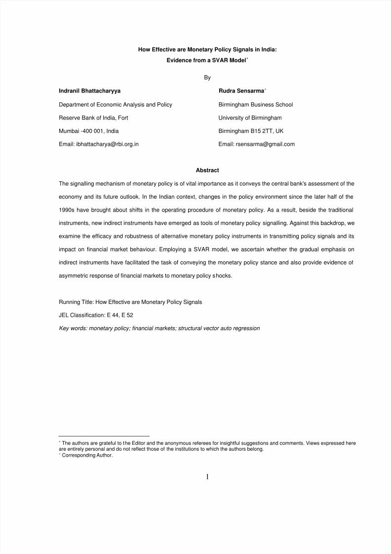
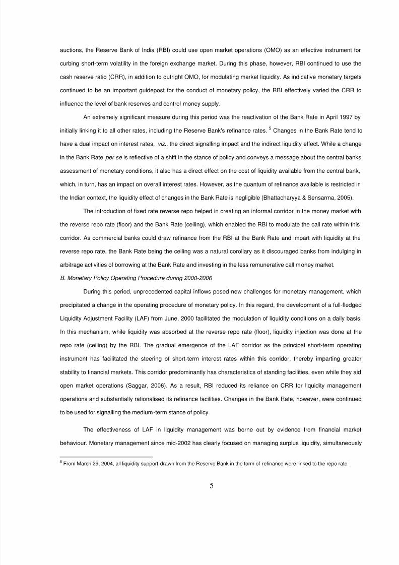
The effectiveness of LAF in liquidity management was borne out by evidence from financial market

behaviour. Monetary management since mid-2002 has clearly focused on managing surplus liquidity, simultaneously

5From March 29, 2004, all liquidity support drawn from the Reserve Bank in the form of refinance were linked to the repo rate.



6

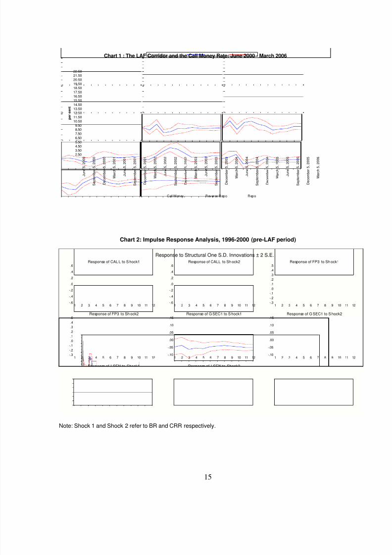
operating through LAF and open market operations. As a result, monthly average call rates, which were volatile

during 1990-98, have stabilised subsequently after the introduction of LAF (Chart 1). The benefits of efficient liquidity

management operations were also apparent from the relatively orderly movement of both the exchange rates and

interest rates during this period.

IV. Empirical Evidence and Policy Implications

Having outlined the contours of the shifts in operating procedure in India’s monetary policy, we now move to

the question of how effective has been the shift in emphasis from quantum to rate instruments. For this purpose, we

empirically examine the effectiveness of monetary policy signals in India over a 10 year period beginning 1996:M04

till 2006:M03 (monthly data)6. We consider the following monetary policy instruments used by the RBI: cash reserve

ratio (CRR), Bank Rate (BR) and reverse repo rate (RRATE). Since the repo auctions started in 2000, we restrict our

analysis involving reverse repo rate to the period 2000:M07 – 2006:M03. Our objective is to assess the impact of

these alternative monetary policy signals on four segments of the financial market, viz . money market, foreign

exchange market, government securities market and stock market. Accordingly, our variables of interest are the call

money rate (CALL), 3-month forward premia (FP3), yield on 1-year government securities (GSEC1) and BSE Sensex

in logarithmic scale (LSEN).7

At the outset, we present some summary statistics in Table 1 to provide a brief idea about the data. We also

computed the pair-wise correlations of the two sets of variables under study and found that the policy variables are

positively correlated with the call money, forward premia and yield rates and negatively correlated with the stock

market index8

.

(Table 1 here)

For the empirical exercise, we use an SVAR approach which uses economic theory to identify the structural

shocks in a multi-variate time-series model. We follow the methodology of Amisano and Gianini (1997), popularly

known as the AB model, which is appropriate for imposing short-run restrictions (since we deal with financial market

interactions where the speed of adjustments is expected to be high). We impose non-recursive restrictions on the

structural parameters for identification such that, monetary policy variable is not contemporaneously affected by

market variables, while the market variables are affected by monetary policy in a particular order as expected from

the transmission mechanism. This follows from the fact that monetary policy signals are seen to first impact the short

term money market, then the forex market followed by the government securities market and finally the stock market.

6 M03 and M04 signify the month of March and April, respectively, based on calendar year. Data has been sourced from theHandbook of Statistics on the Indian Economy 2005-06.7

We alternatively tried with 6-month forward premia and yield on 10-year government securities. The results were largely the samebut weaker.8

To save space, the correlation matrix is not reported here. I t is available on request.



7

Our empirical strategy is as follows. First, we specify the variables to be included in the model and estimate

the reduced form VAR. We do not conduct unit root tests, but carry out our analysis with the variables in levels

because in case the variables are found to be non-stationary, they would have to be differenced leading to loss of

information.9

The appropriate lag order for the VAR is selected based on sequential LR tests and diagnostic tests for

the presence of autocorrelation and heteroscedasticity in the residuals. We impose restrictions on the appropriate

coefficients of the system so as to have a SVAR with the following order: [Policy Instruments, CALL FP3, GSEC1,

LSEN]. Once the SVAR is identified, we present the impulse response analysis which reports the dynamic response

of each variable to shocks in different equations of the VAR system within two standard error bands (shown as dotted

lines). Finally, we compute forecast error variance decomposition which provides the proportion of the total

forecast-error variance of each variable that is caused by each of the shocks or disturbances in the system.

We conduct the empirical exercises on two periods separately, viz . the pre-LAF period of 1996:04 –2000:06

and then the post-LAF period of 2000:07 –2006:03. Accordingly, we first discuss the results for the pre-LAF period

and then move on to the post-LAF period.

A. 1996:04 – 2000:06

In this period, Bank Rate was reactivated as the signalling instrument by the RBI to communicate its policy

stance to the financial markets while CRR was used for modulating market liquidity. Hence, we consider the impact of

changes in Bank Rate and CRR on various segments of financial market for which we construct a SVAR with the

following order: [BR, CRR, CALL, FP3, GSEC1, LSEN]. Optimal lag order selected was 3 such that no

autocorrelation or heteroscedasticity is detected from the LM and White’s tests, respectively. We do not present the

estimated model here since our interest is in the impact of shocks. However, we do present VAR estimates later while

studying asymmetry through the use of a dummy variable and the results are not very different from those with the

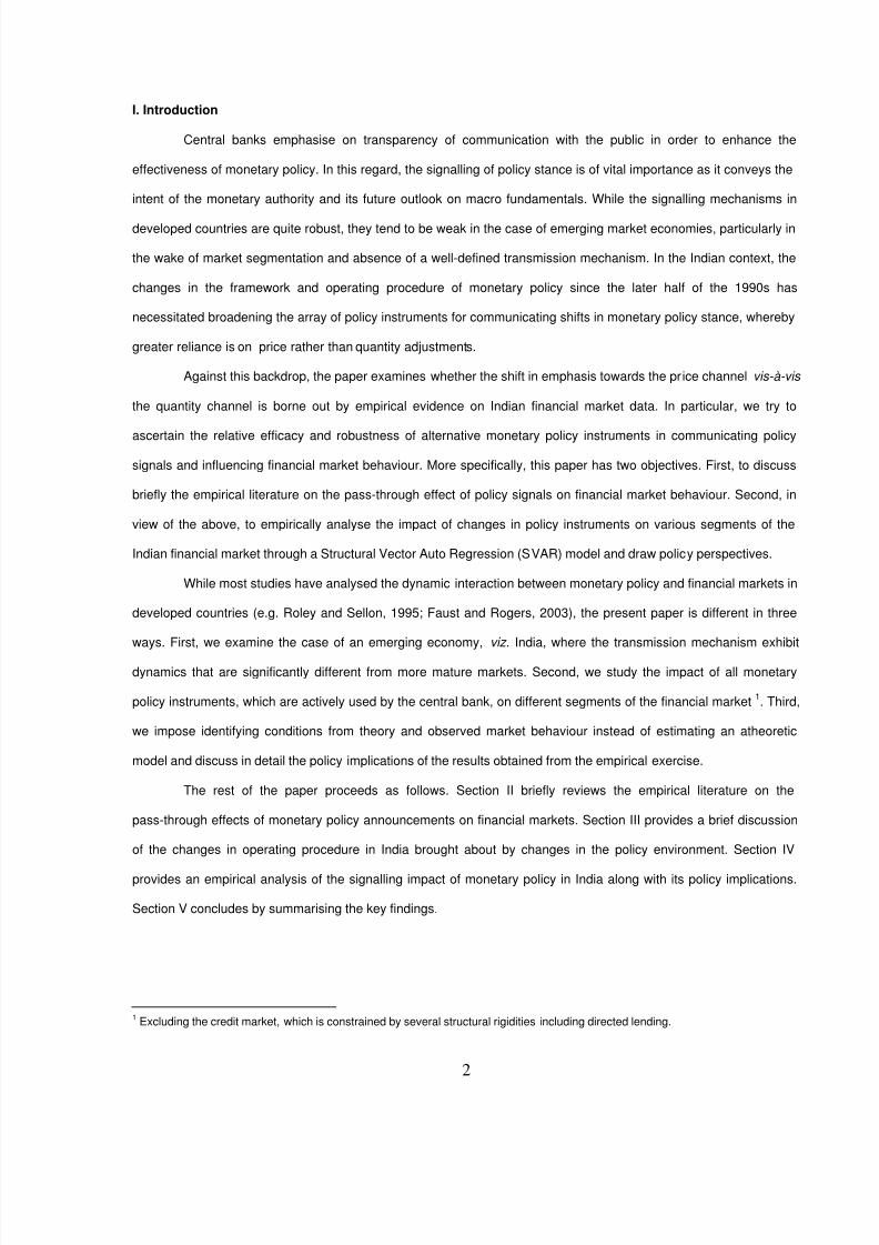
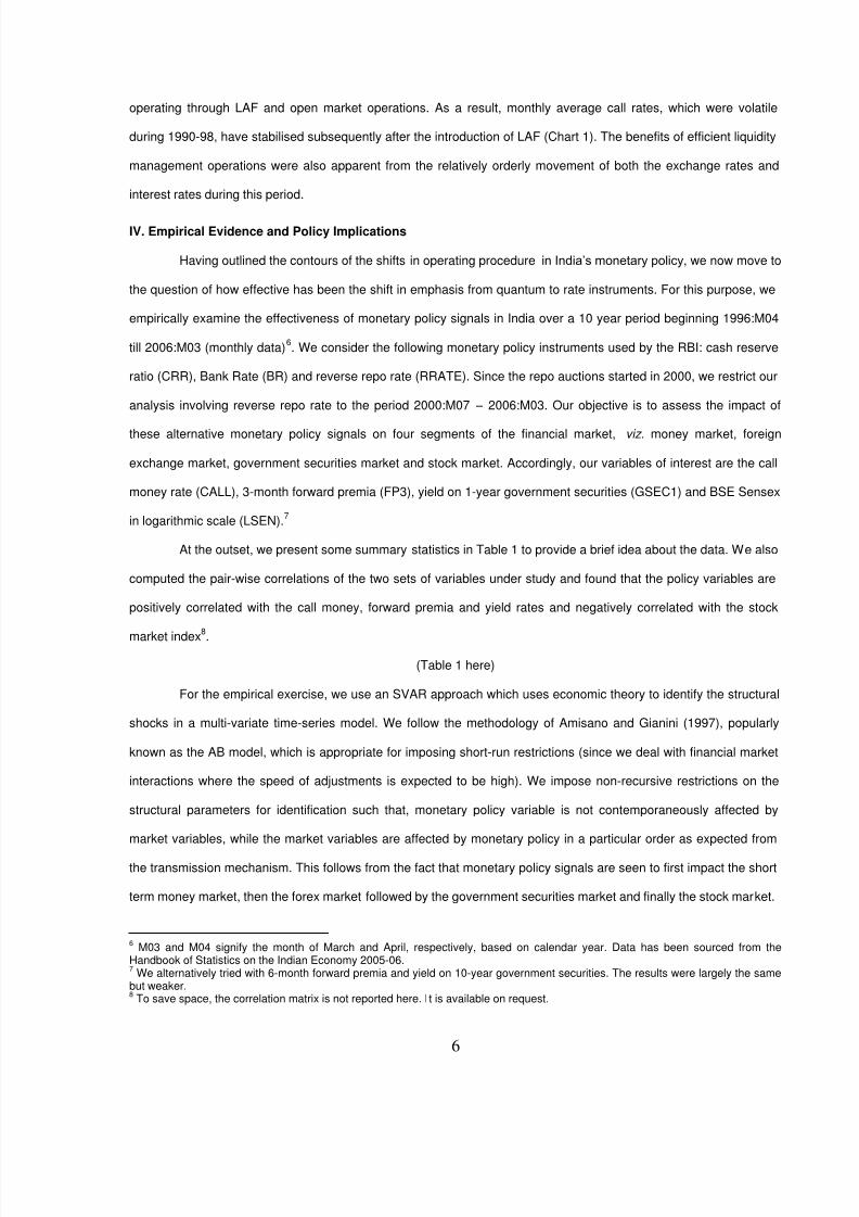
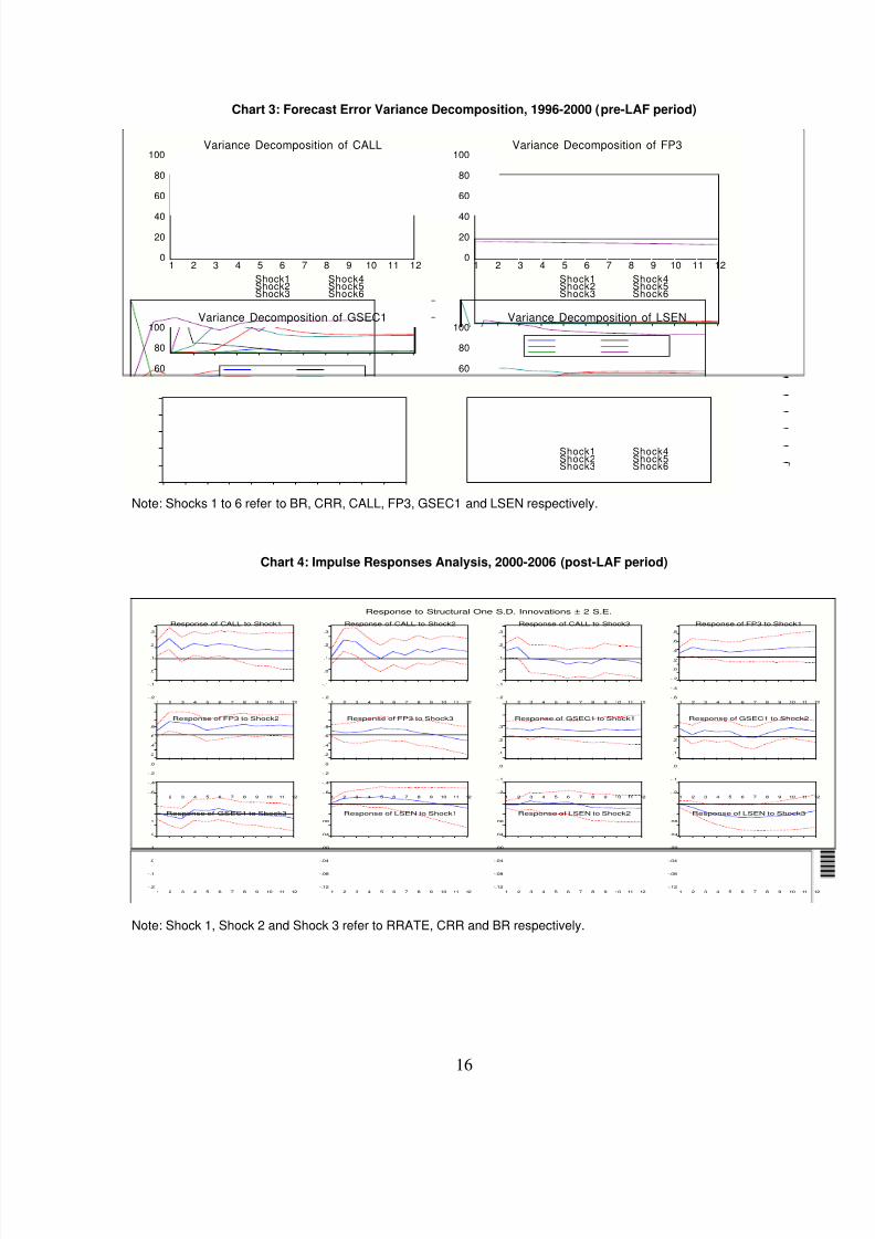
present specification. We directly move to the impulse response analysis (Chart 2) which suggests the following.

Impact of BR on CALL fluctuates between negative and positive values, eventually dying out in around 7

months. However the strength of the impact is not very significant as suggested by the standard error bands. Impact

of CRR on CALL is positive and significant, and dies out in around 10 months. Impact of BR on FP3 is negative and

substantial only in the fourth and fifth months. Although this may appear to be counterintuitive, one explanation might

be that an increase in Bank Rate would increase interest rates leading to a widening of the interest rate differential.

9According to Brooks (2002), a SVAR in differences would lead to losing information on the co-movement among the variables

which is our primary interest. Sims, Stock and Watson (1990) report that VARs with non-stationary variables incur some loss in theestimator’s efficiency but not consistency. Even in case of loss in efficiency of estimates, Sims (1980) recommended againstdifferencing the variables since the goal of VAR analysis is to study inter-relationships and not determine efficient estimates.Furthermore, in our case, it would not be economically meaningful to define differences in some financial market rates and notothers, while studying their inter-relationships. This could have been a problem as, in the Indian case, call money rates have beenfound to be stationary unlike the other rates which are non-stationary (Bhattacharya and Sensarma, op cit ).



8

Consequently, it would attract more capital inflows leading to expectation of an appreciation of the rupee and

consequently a decline in the forward premia on foreign currency. However, with sterilised intervention by the RBI in

the long run, the appreciation is neutralised and the tightness in liquidity results in an increase in the forward premia.

The strength of the impact, however, is not very significant. The impact of CRR on FP3 is positive and significant, and

persistent beyond 12 months. Impact of BR and CRR, respectively, on GSEC1 is negligible (except for a positive

impact of CRR around the fifth and sixth months), and that on LSEN is negligible as well.

(Chart 2 here)

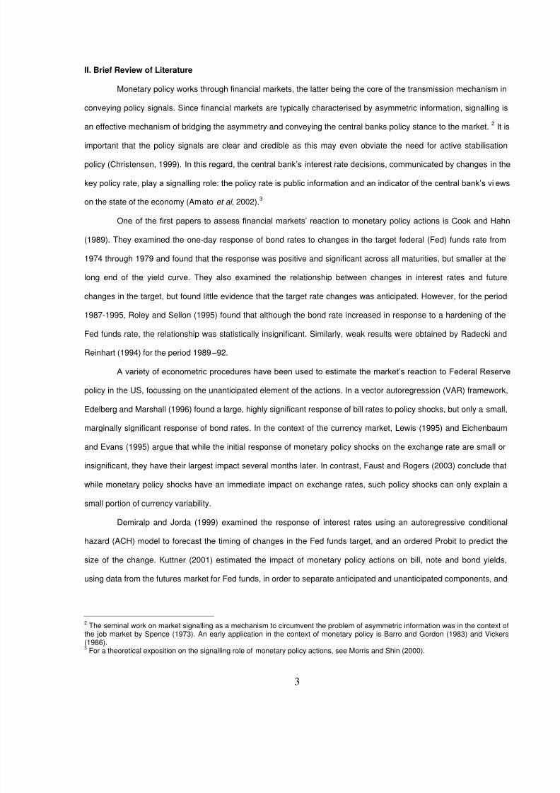
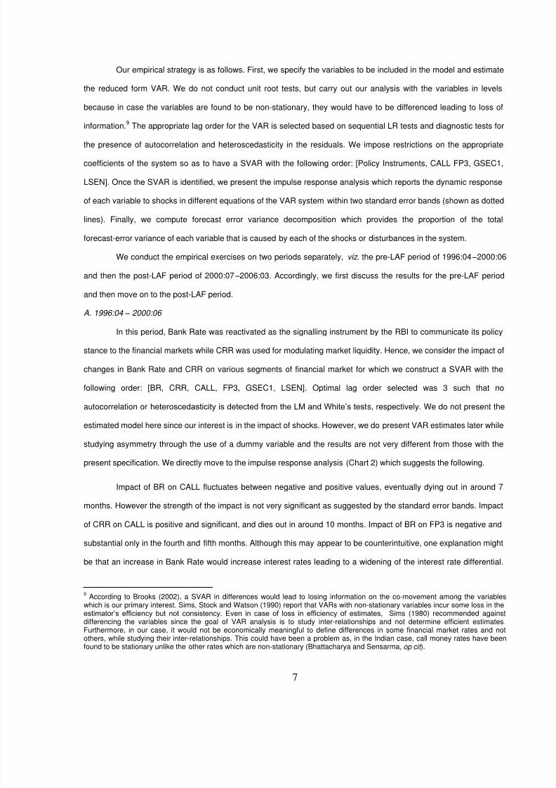
Forecast Error Variance Decomposition analysis (Chart 3) suggests that variations in CALL are most

explained by LSEN, CRR, BR, GSEC1, FP3, and CALL in this order. Thus, CRR appears to have played a more

dominant role as compared with Bank Rate. Same is the case with FP3 whose variations are most explained by

LSEN, CRR, GSEC1, FP3, BR, and CALL in this order. Variations in GSEC1 are most explained by LSEN, GSEC1,

CRR, BR, FP3, and CALL in this order. Finally, variations in LSEN are most explained by LSEN, CRR, FP3, GSEC1,

CALL, and BR in this order. Thus in case of all financial market segments, CRR has been the more potent monetary

policy signal than the Bank Rate during the pre-LAF period.

(Chart 3 here)

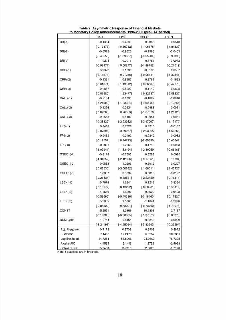
In the above model, we experimented with a dummy variable (DUM) for monetary policy regime that takes

the value one during the period of an expansionary monetary policy. We define the dummy variable as taking the

value one whenever there is a reduction in the CRR (as CRR was largely rationalised during this period) and in the

subsequent periods till there is a policy reversal. Similarly, the dummy variable takes the value zero whenever there

is an increase in the CRR and in the subsequent periods till there is a policy reversal. Next, we interacted this dummy

variable with CRR to create DUM*CRR whose coefficient indicates whether the impact of a rise in CRR is different

from that of a fall in CRR. The estimated VAR model is presented in Table 2. In all cases except for the stock market,

the coefficient of DUM*CRR is negative and statistically significant. This result indicates that when there is a

reduction in CRR (expansionary monetary policy); the consequent decline in the market rates is lower in absolute

terms than the impact of an increase in CRR. This suggests the presence of asymmetric response of markets to

monetary policy changes in India during this period. Specifically, an expansionary policy appears to have had a

weaker impact on various markets than a contractionary policy. This result is similar to the evidence provided by

Vähämaa (op cit ) and Lobo et al (op cit ) for bond and forex markets respectively. We are able to extend the evidence

to the money market as well in the Indian context.

(Table 2 here)



9

B. 2000:07 – 2006:03

Here, we consider the impact of changes in the reverse repo rate, CRR and Bank Rate on various segments

of financial market for which we construct a SVAR with the following order: [RRATE, CRR, BR, CALL, FP3, GSEC1,

LSEN]. Optimal lag order selected was 2 such that no autocorrelation or heteroscedasticity is detected from the LM

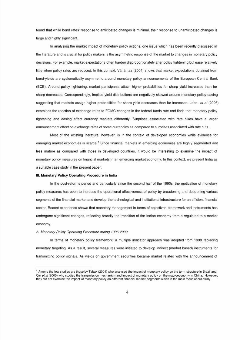
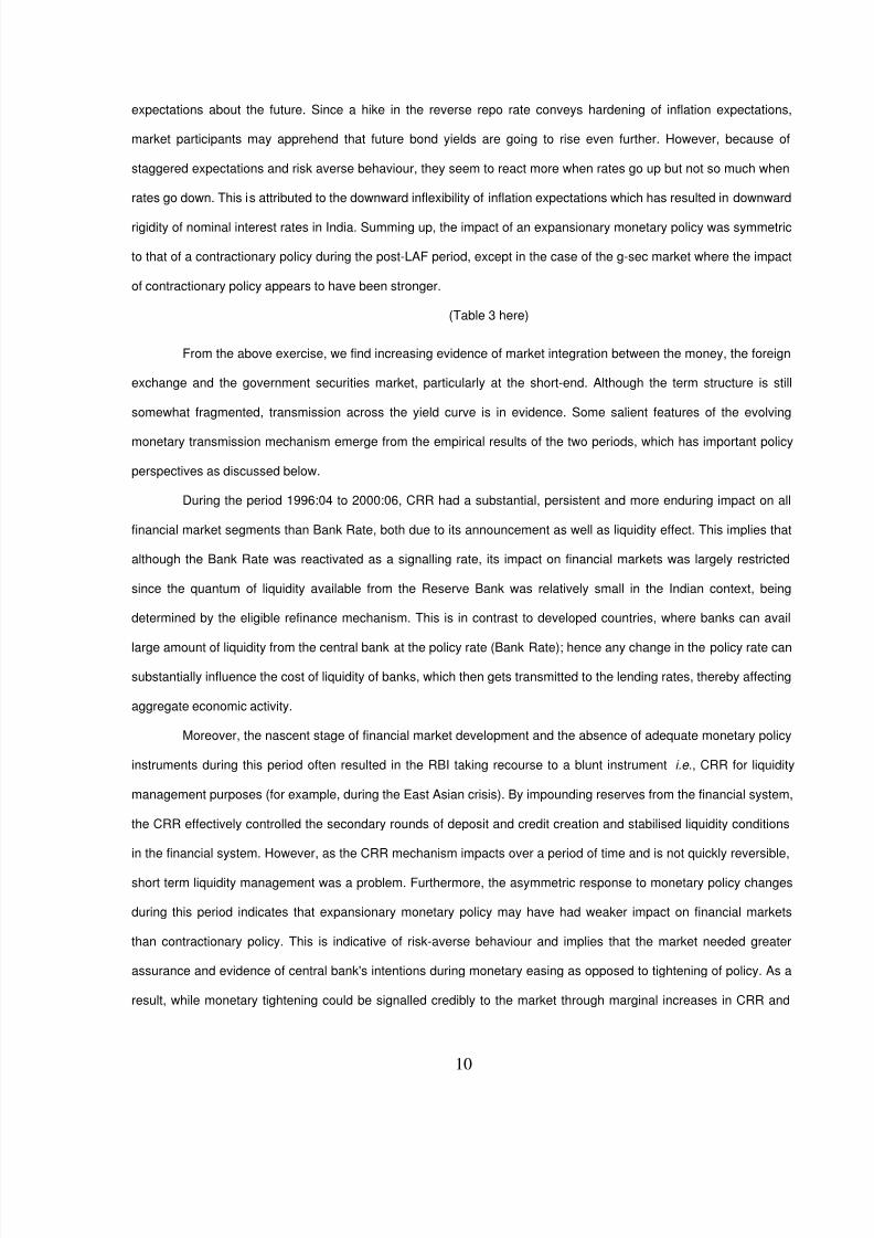
and White’s tests, respectively. The impulse response analysis (Chart 4) suggests the following. Impact of RRATE on

CALL is positive and significant but dies out in around 7 months. Impact of CRR on CALL is positive until 4 months

and negligible thereafter. Impact of BR on CALL is negligible. Impact of RRATE and CRR on FP3 is positive and

persistent (even though the strength of the impacts is not very significant beyond a few months), whereas the impact

of BR is weak but positive till 8 months and turns negative thereafter. Impact of RRATE on GSEC1 is marginally

positive whereas that of CRR and BR is negligible. Impact of RRATE, CRR and BR on LSEN is negligible.

(Chart 4 here)

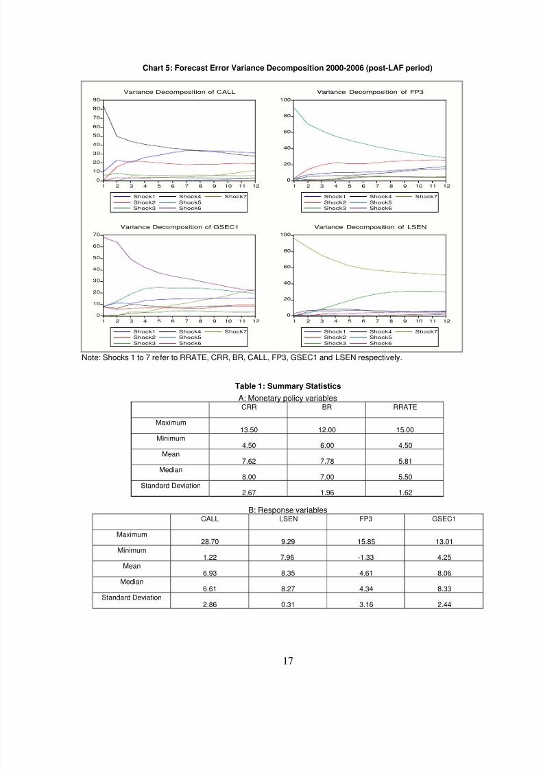
Forecast Error Variance Decomposition analysis (Chart 5) suggests the following. Variations in CALL are

most explained by CALL, RRATE, CRR, GSEC1, FP3, BR, and LSEN in this order. Thus, reverse repo rate appears

to be the most potent policy variable in the post-LAF period. This is also evident from the variations in FP3 which are

most explained by FP3, RRATE, CRR, CALL, BR, LSEN, GSEC1 in this order. Similarly, variations in GSEC1 are

most explained by GSEC1, FP3, RRATE, LSEN, CALL, CRR and BR in this order. Variations in LSEN, however, are

most explained by LSEN, BR, CALL, RRATE, GSEC1, CRR and FP3 in this order. Thus, except for the stock market,

reverse repo rate appears to have played the dominant role in transmitting monetary policy signals to various

financial market segments during this period.

(Chart 5 here)

In the above exercise, we once again experimented with a monetary policy regime dummy variable as

before. In this case, we define the dummy variable as taking the value one whenever there is a fall in the reverse

repo rate (since we are considering the post-LAF period of 2000-06) and in the subsequent periods till there is a

policy reversal. Similarly, the dummy variable takes the value zero whenever there is a rise in the policy rate and in

the subsequent periods till there is a policy reversal. Next, we interacted this dummy variable with RRATE to create

DUM*RRATE whose coefficient would tell us whether the impact of a rise in the RRATE is different from that of a fall

in the RRATE. The estimated VAR model is presented in Table 3. In this case, however, the interaction variable had

a significant coefficient only for GSEC1 i.e. we are able to provide evidence for asymmetric impact of monetary policy

changes only in the government securities market during the post-LAF period. That the asymmetry is getting reflected

only in the g-sec (government securities) market is not surprising as movement in bond yields are largely based on



10

expectations about the future. Since a hike in the reverse repo rate conveys hardening of inflation expectations,

market participants may apprehend that future bond yields are going to rise even further. However, because of

staggered expectations and risk averse behaviour, they seem to react more when rates go up but not so much when

rates go down. This is attributed to the downward inflexibility of inflation expectations which has resulted in downward

rigidity of nominal interest rates in India. Summing up, the impact of an expansionary monetary policy was symmetric

to that of a contractionary policy during the post-LAF period, except in the case of the g-sec market where the impact

of contractionary policy appears to have been stronger.

(Table 3 here)

From the above exercise, we find increasing evidence of market integration between the money, the foreign

exchange and the government securities market, particularly at the short-end. Although the term structure is still

somewhat fragmented, transmission across the yield curve is in evidence. Some salient features of the evolving

monetary transmission mechanism emerge from the empirical results of the two periods, which has important policy

perspectives as discussed below.

During the period 1996:04 to 2000:06, CRR had a substantial, persistent and more enduring impact on all

financial market segments than Bank Rate, both due to its announcement as well as liquidity effect. This implies that

although the Bank Rate was reactivated as a signalling rate, its impact on financial markets was largely restricted

since the quantum of liquidity available from the Reserve Bank was relatively small in the Indian context, being

determined by the eligible refinance mechanism. This is in contrast to developed countries, where banks can avail

large amount of liquidity from the central bank at the policy rate (Bank Rate); hence any change in the policy rate can

substantially influence the cost of liquidity of banks, which then gets transmitted to the lending rates, thereby affecting

aggregate economic activity.

Moreover, the nascent stage of financial market development and the absence of adequate monetary policy

instruments during this period often resulted in the RBI taking recourse to a blunt instrument i.e ., CRR for liquidity

management purposes (for example, during the East Asian crisis). By impounding reserves from the financial system,

the CRR effectively controlled the secondary rounds of deposit and credit creation and stabilised liquidity conditions

in the financial system. However, as the CRR mechanism impacts over a period of time and is not quickly reversible,

short term liquidity management was a problem. Furthermore, the asymmetric response to monetary policy changes

during this period indicates that expansionary monetary policy may have had weaker impact on financial markets

than contractionary policy. This is indicative of risk-averse behaviour and implies that the market needed greater

assurance and evidence of central bank's intentions during monetary easing as opposed to tightening of policy. As a

result, while monetary tightening could be signalled credibly to the market through marginal increases in CRR and



11

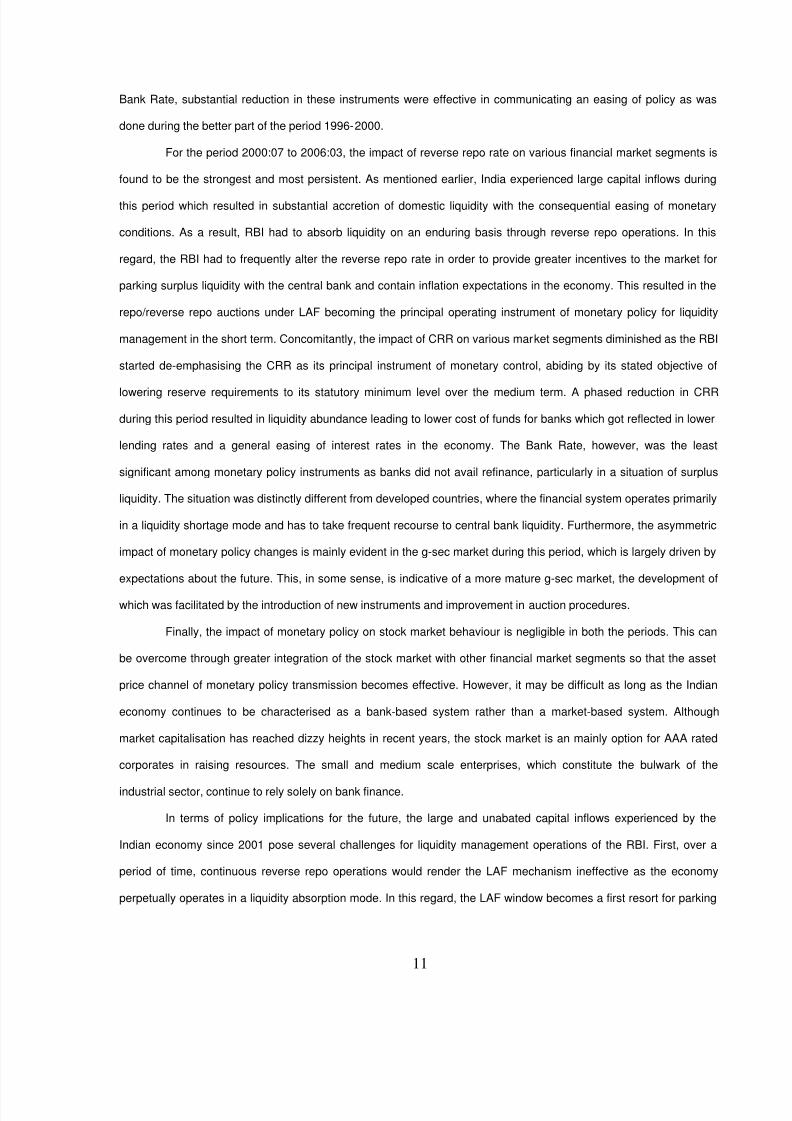
Bank Rate, substantial reduction in these instruments were effective in communicating an easing of policy as was

done during the better part of the period 1996-2000.

For the period 2000:07 to 2006:03, the impact of reverse repo rate on various financial market segments is

found to be the strongest and most persistent. As mentioned earlier, India experienced large capital inflows during

this period which resulted in substantial accretion of domestic liquidity with the consequential easing of monetary

conditions. As a result, RBI had to absorb liquidity on an enduring basis through reverse repo operations. In this

regard, the RBI had to frequently alter the reverse repo rate in order to provide greater incentives to the market for

parking surplus liquidity with the central bank and contain inflation expectations in the economy. This resulted in the

repo/reverse repo auctions under LAF becoming the principal operating instrument of monetary policy for liquidity

management in the short term. Concomitantly, the impact of CRR on various market segments diminished as the RBI

started de-emphasising the CRR as its principal instrument of monetary control, abiding by its stated objective of

lowering reserve requirements to its statutory minimum level over the medium term. A phased reduction in CRR

during this period resulted in liquidity abundance leading to lower cost of funds for banks which got reflected in lower

lending rates and a general easing of interest rates in the economy. The Bank Rate, however, was the least

significant among monetary policy instruments as banks did not avail refinance, particularly in a situation of surplus

liquidity. The situation was distinctly different from developed countries, where the financial system operates primarily

in a liquidity shortage mode and has to take frequent recourse to central bank liquidity. Furthermore, the asymmetric

impact of monetary policy changes is mainly evident in the g-sec market during this period, which is largely driven by

expectations about the future. This, in some sense, is indicative of a more mature g-sec market, the development of

which was facilitated by the introduction of new instruments and improvement in auction procedures.

Finally, the impact of monetary policy on stock market behaviour is negligible in both the periods. This can

be overcome through greater integration of the stock market with other financial market segments so that the asset

price channel of monetary policy transmission becomes effective. However, it may be difficult as long as the Indian

economy continues to be characterised as a bank-based system rather than a market-based system. Although

market capitalisation has reached dizzy heights in recent years, the stock market is an mainly option for AAA rated

corporates in raising resources. The small and medium scale enterprises, which constitute the bulwark of the

industrial sector, continue to rely solely on bank finance.

In terms of policy implications for the future, the large and unabated capital inflows experienced by the

Indian economy since 2001 pose several challenges for liquidity management operations of the RBI. First, over a

period of time, continuous reverse repo operations would render the LAF mechanism ineffective as the economy

perpetually operates in a liquidity absorption mode. In this regard, the LAF window becomes a first resort for parking



12

surplus funds as banks end up quoting the LAF rate in auctions. Thus, the variable reverse repo rate defacto

becomes a fixed repo rate. Furthermore, the resources absorbed under LAF flows back into the system during the

reverse leg of the transaction, as a result the economy is saddled with a perpetual liquidity overhang. In this context,

while the stated objective is to absorb temporary liquidity through LAF and the more permanent liquidity through

market stabilisation scheme (MSS) securities, there is no way of knowing ex-ante whether the liquidity situation is

temporary or permanent. Second, RBI may not be in a position to conduct sterilisation operations indefinitely as its

inventory of government paper gradually gets depleted, nor would it be able to increase the stock of government

paper as it has fiscal ramifications10

. This has been further compounded by RBI's withdrawal from primary market

auctions of government paper from April, 2006 as per the stipulations of the Fiscal Responsibility and Budget

Management (FRBM) Act (2004). In such a scenario, and notwithstanding the RBI’s long run goal of reducing it to the

statutory minimum level, the CRR would continue to be one of the most potent instruments for liquidity absorption

given the nascent state of development of market based monetary policy instruments. Finally, there is a need to

rethink the role of the Bank Rate, particularly in a situation of surplus liquidity. It has been argued that, ideally, there

should be one rate at which liquidity is injected or absorbed. At present, the situation is somewhat anomalous in that

liquidity injection is done both at the Bank Rate and the Repo Rate. One possible solution could be to align the Bank

Rate with the Repo Rate given that the liquidity impact of the Bank Rate is not significant in the Indian context. All

these would remain vexing issues for the RBI's monetary and liquidity management operations, particularly as it

continues to grapple with a situation of surplus liquidity in the foreseeable future.

V. Concluding Observations

Our analysis suggests that even though the Bank Rate was identified by the RBI as the principal signalling

instrument in the pre-LAF period, quantity adjustments through CRR had a dominant impact on financial markets vis-

à-vis rate instruments. In the post-LAF period, however, the situation changed as the reverse repo rate became the

most important signalling rate of the RBI. The impact of these signalling instruments, however, was confined to the

money, forex and bond markets leaving the stock market largel y unaffected. Thus, while the RBI’s policy actions had

an impact in most segments of the financial market in India, its impact on the stock market was negligible. For the

remaining segments of the financial market, we are able to provide empirical evidence on the effectiveness of

monetary policy signals, both in the pre and post-LAF periods and the asymmetric impact of monetary policy

announcements on financial markets, albeit somewhat muted in the post-LAF period .

10 Unlike in some other countries, the RBI is not empowered to float its own security.



13

References

1. Amato, J. D., Morris, S., & Shin, H. S. (2002) Communication and Monetary Policy. Oxford Review of

Economic Policy 18(4): 495-503.

2. Amisano, G., & Gianini, C. (1997). Topics in Structural VAR Econometrics . Berlin: Springer-Verlag.

3. Barro, R. & Gordon, D. (1983). A Positive Theory of Monetary Policy in a Natural Rate Model. Journal of

Political Economy , 91: 589 – 610.

4. Bhattacharyya, I. & Sensarma, R. (2005). Signalling Instruments of Monetary Policy: The Indian Experience.

Journal of Quantitative Economics , 3(2): 180-196.

5. Brooks, C. (2002). Introductory Econometrics for Finance . Cambridge: Cambridge University Press.

6. Christensen, M. (1999). Credibility of Policy Announcements Under Asymmetric Information. Journal of

Policy Modeling , 21(6): 747 –751.

7. Cook, T. & Hahn, T. (1989). The Effect of Changes in the Federal Funds Rate Target on Market Interest

Rates in the 1970s. Journal of Monetary Economics , 24: 331 –351.

8. Demiralp, S. & Oscar, J. (1999). The Transmission of Monetary Policy via Announcement Effects.

Unpublished Manuscript , University of California Davis.

9. Edelberg, W. & Marshall, D. (1996). Monetary Policy Shocks and Long-Term Interest Rates. Federal

Reserve Bank of Chicago Economic Perspectives , 20(2): 2 –1

10. Eichenbaum, M. & Evans, C. L. (1995). Some empirical evidence on the effects of shocks to monetary policy

on exchange rates. Quarterly Journal of Economics, 110: 975-1009.

11. Faust, J. & Rogers, J. H. (2003). Monetary policy’s role in exchange rate behaviour . Journal of Monetary

Economics , 50: 1403-1424.

12. Kuttner, K. N. (2001). Monetary policy surprises and interest rates: Evidence from the Fed funds future

market. Journal of Monetary Economics , 47: 523-544.

13. Lewis, K. K. (1995). Are Foreign Exchange Intervention and Monetary Policy Related, and Does it Really

Matter. Journal of Business , 68(2): 185-214.

14. Lobo, B. J., Darrat, A. F. & Ramchander, S. (2006). The Asymmetric Impact of Monetary Policy on Currency

Markets. forthcoming in The Financial Review .

15. Morris, S. & Shin, H. S. (2002). Social Value of Public Information. American Economic Review . 52: 1521-34

16. Qin, D., Quising, P., He, X.& Liu, S. (2005). Modeling monetary transmission and policy in China. Journal of

Policy Modeling, 27(2): 157-175.



14

17. Radecki, L. & Reinhart, V. (1994). The Financial Linkages in the Transmission of Monetary Policy in the

United States. in National Differences in Interest Rate Transmission . Bank for International Settlements.

18. Roley, V. V. & Sellon, G. H. (1995). Monetary Policy Actions and Long Term Interest Rates. Federal

Reserve Bank of Kansas City Economic Quarterly , 80(4): 77 –89.

19. Saggar, M. (2006). Monetary Policy and Operations in Countries with Surplus Liquidity. Economic and

Political Weekly , March 18: 1041-1052.

20. Sims, C. A. (1980). Macroeconomics and reality. Econometrica , 48: 1-49.

21. Sims, C. A., Stock, J. H. & Watson, M. W. (1990). Inference in Linear Time Series Models with Some Unit

Roots. Econometrica , 58(1): 113-44.

22. Spence, M. (1973). Job market signaling. Quarterly Journal of Economics , 87: 296-332.

23. Tabak, B. M. (2004). A note on the effects of monetary policy surprises on the Brazilian term structure of

interest rates. Journal of Policy Modeling, 26(3): 283-287.

24. Vähämaa, S. (2004). Option-implied asymmetries in bond market expectations around monetary policy

actions of the ECB. ECB Working Paper No. 315.

25. Vickers, J. (1986). Signalling in a Model of Monetary Policy with Incomplete Information. Oxford Economic

Papers, 38: 443-455.



15

Chart 1 : The LAF Corridor and the Call Money Rate: June 2000 - March 2006

2.50

3.50

4.50

5.50

6.50

7.50

8.509.50

10.50

11.50

12.5013.50

14.50

15.5016.50

17.50

18.50

19.50

20.50

21.5022.50

J u n e 5 ,

2 0 0 0

S e p t e m b e r 5 ,

2 0 0 0

D e c e m b e r 5 ,

2 0 0 0

M a r c h 5 ,

2 0 0 1

J u n e 5 ,

2 0 0 1


2 0 0 1

D e c e m b e r 5 ,

2 0 0 1

M a r c h 5 ,

2 0 0 2

J u n e 5 ,

2 0 0 2


2 0 0 2

D e c e m b e r 5 ,

2 0 0 2

M a r c h 5 ,

2 0 0 3

J u n e 5 ,

2 0 0 3


2 0 0 3

D e c e m b e r 5 ,

2 0 0 3

M a r c h 5 ,

2 0 0 4

J u n e 5 ,

2 0 0 4


2 0 0 4

D e c e m b e r 5 ,

2 0 0 4

M a r c h 5 ,

2 0 0 5

J u n e 5 ,

2 0 0 5


2 0 0 5

D e c e m b e r 5 ,

2 0 0 5

M a r c h 5 ,

2 0 0 6

p e r c e n t

Cal l Money Reverse Repo Repo

Chart 2: Impulse Response Analysis, 1996-2000 (pre-LAF period)

-.6

-.4-.2

.0

.2

.4

.6

1 2 3 4 5 6 7 8 9 10 11 12

Response of CAL L to S hock1

-.6

-.4-.2

.0

.2

.4

.6

1 2 3 4 5 6 7 8 9 10 11 12

Response of CALL to Sh ock2

-.3

-.2

-.1

.0

.1

.2

.3

.4

.5

1 2 3 4 5 6 7 8 9 10 11 12

Response of FP3 to Sh ock1

-.3

-.2

-.1

.0

.1

.2

.3

.4

.5

1 2 3 4 5 6 7 8 9 10 11 12

Response of FP3 to Sh ock2

-.10

-.05

.00

.05

.10

.15

1 2 3 4 5 6 7 8 9 10 11 12

Response of G SEC1 to S hock1

-.10

-.05

.00

.05

.10

.15

1 2 3 4 5 6 7 8 9 10 11 12

Response of G SEC1 to S hock2

-.06

-.04

-.02

.00

.02

.04

1 2 3 4 5 6 7 8 9 10 11 12

Response of LSEN to Shock1

-.06

-.04

-.02

.00

.02

.04

1 2 3 4 5 6 7 8 9 10 11 12


Response to Structural One S.D. Innovations ± 2 S.E.

Note: Shock 1 and Shock 2 refer to BR and CRR respectively.



16

Chart 3: Forecast Error Variance Decomposition, 1996-2000 (pre-LAF period)

0

20

40

60

80

100

1 2 3 4 5 6 7 8 9 10 11 12

Shock1Shock2Shock3

Shock4Shock5Shock6

Variance Decomposition of CALL

0

20

40

60

80

100

1 2 3 4 5 6 7 8 9 10 11 12

Shock1Shock2Shock3

Shock4Shock5Shock6

Variance Decomposition of FP3

0

20

40

60

80

100

1 2 3 4 5 6 7 8 9 10 11 12

Shock1Shock2Shock3

Shock4Shock5Shock6

Variance Decomposition of GSEC1

0

20

40

60

80

100

1 2 3 4 5 6 7 8 9 10 11 12

Shock1Shock2Shock3

Shock4Shock5Shock6

Variance Decomposition of LSEN

Note: Shocks 1 to 6 refer to BR, CRR, CALL, FP3, GSEC1 and LSEN respectively.

Chart 4: Impulse Responses Analysis, 2000-2006 (post-LAF period)

-.2

-.1

.0

.1

.2

.3

1 2 3 4 5 6 7 8 9 10 11 12

Response of CALL to Shock1

-.2

-.1

.0

.1

.2

.3

1 2 3 4 5 6 7 8 9 10 11 12


-.2

-.1

.0

.1

.2

.3

1 2 3 4 5 6 7 8 9 10 11 12


-.6

-.4

-.2

.0

.2

.4

.6

.8

1 2 3 4 5 6 7 8 9 10 11 12

Response of FP3 to Shock1

-.6

-.4

-.2

.0

.2

.4

.6

.8

1 2 3 4 5 6 7 8 9 10 11 12


-.6

-.4

-.2

.0

.2

.4

.6

.8

1 2 3 4 5 6 7 8 9 10 11 12


-.2

-.1

.0

.1

.2

.3

1 2 3 4 5 6 7 8 9 10 11 12

Response of GSEC1 to Shock1

-.2

-.1

.0

.1

.2

.3

1 2 3 4 5 6 7 8 9 10 11 12


-.2

-.1

.0

.1

.2

.3

1 2 3 4 5 6 7 8 9 10 11 12


-.12

-.08

-.04

.00

.04

.08

1 2 3 4 5 6 7 8 9 10 11 12


-.12

-.08

-.04

.00

.04

.08

1 2 3 4 5 6 7 8 9 10 11 12


-.12

-.08

-.04

.00

.04

.08

1 2 3 4 5 6 7 8 9 10 11 12


Response to Structural One S.D. Innovations ± 2 S.E.

Note: Shock 1, Shock 2 and Shock 3 refer to RRATE, CRR and BR respectively.



17

Chart 5: Forecast Error Variance Decomposition 2000-2006 (post-LAF period)

0

10

20

30

40

50

60

70

80

90

1 2 3 4 5 6 7 8 9 10 11 12

Shock1

Shock2

Shock3

Shock4

Shock5

Shock6

Shock7

Variance Decomposition of CALL

0

20

40

60

80

100

1 2 3 4 5 6 7 8 9 10 11 12

Shock1

Shock2

Shock3

Shock4

Shock5

Shock6

Shock7

Variance Decomposition of FP3

0

10

20

30

40

50

60

70

1 2 3 4 5 6 7 8 9 10 11 12

Shock1

Shock2

Shock3

Shock4

Shock5

Shock6

Shock7

Variance Decomposition of GSEC1

0

20

40

60

80

100

1 2 3 4 5 6 7 8 9 10 11 12

Shock1

Shock2

Shock3

Shock4

Shock5

Shock6

Shock7

Variance Decomposition of LSEN

Note: Shocks 1 to 7 refer to RRATE, CRR, BR, CALL, FP3, GSEC1 and LSEN respectively.

Table 1: Summary Statistics

A: Monetary policy variablesCRR BR RRATE

Maximum13.50 12.00 15.00

Minimum4.50 6.00 4.50

Mean7.62 7.78 5.81

Median8.00 7.00 5.50

Standard Deviation2.67 1.96 1.62

B: Response variablesCALL LSEN FP3 GSEC1

Maximum28.70 9.29 15.85 13.01

Minimum1.22 7.96 -1.33 4.25

Mean6.93 8.35 4.61 8.06

Median6.61 8.27 4.34 8.33

Standard Deviation2.86 0.31 3.16 2.44



18

Table 2: Asymmetric Response of Financial Marketsto Monetary Policy Announcements, 1996-2000 (pre-LAF period)

CALL FP3 GSEC1 LSEN

BR(-1) -0.1354 0.4393 0.2868 0.0548

[-0.13876] [ 0.86782] [ 1.06878] [ 1.81837]

BR(-2) -0.6512 -0.9523 -0.1996 -0.0403

[-0.49553] [-1.39667] [-0.55204] [-0.99398]BR(-3) -1.0304 0.0016 -0.5786 -0.0072

[-0.92471] [ 0.00277] [-1.88782] [-0.21019]

CRR(-1) 3.9372 0.1396 -0.0196 0.0537

[ 3.11573] [ 0.21286] [-0.05641] [ 1.37548]

CRR(-2) -0.9321 0.8886 0.2769 -0.1623

[-0.61674] [ 1.13312] [ 0.66607] [-3.47778]

CRR(-3) 0.0857 0.8220 0.1140 0.0825

[ 0.06680] [ 1.23477] [ 0.32287] [ 2.08337]

CALL(-1) -0.7184 -0.1095 -0.1697 -0.0010

[-4.21900] [-1.23924] [-3.62239] [-0.19264]

CALL(-2) 0.1356 0.0224 -0.0483 0.0061

[ 0.82688] [ 0.26353] [-1.07070] [ 1.20126]

CALL(-3) -0.0543 -0.1480 -0.0954 0.0051

[-0.38829] [-2.03952] [-2.47997] [ 1.17170]

FP3(-1) 0.3486 0.7629 0.3215 -0.0187

[ 0.87505] [ 3.69077] [ 2.93365] [-1.52366]

FP3(-2) -0.0482 0.0492 -0.2849 0.0052

[-0.12552] [ 0.24713] [-2.69836] [ 0.43641]

FP3(-3) -0.2861 0.2068 0.1718 -0.0053

[-1.09941] [ 1.53194] [ 2.40059] [-0.66466]

GSEC1(-1) -0.8118 -0.7596 0.0283 0.0020

[-1.34652] [-2.42826] [ 0.17061] [ 0.10734]

GSEC1(-2) 0.0563 -1.0296 0.3012 0.0297

[ 0.08530] [-3.00882] [ 1.66011] [ 1.45920]

GSEC1(-3) 1.8887 0.3832 0.5815 -0.0197

[ 2.26434] [ 0.88551] [ 2.53420] [-0.76314]

LSEN(-1) 0.7678 1.2344 0.9218 0.9384

[ 0.13972] [ 0.43292] [ 0.60981] [ 5.53119]

LSEN(-2) -4.5650 -1.6297 -0.3522 0.0428

[-0.58696] [-0.40386] [-0.16460] [ 0.17820]

LSEN(-3) 5.2035 1.5063 -1.1044 -0.2926

[ 0.95520] [ 0.53291] [-0.73700] [-1.73975]

CONST -5.2551 -1.3366 10.9803 2.7187

[-0.18086] [-0.08865] [ 1.37373] [ 3.03070]

DUM*CRR -1.9744 -0.6154 -0.3843 -0.0029

[-8.24193] [-4.95094] [-5.83242] [-0.39594]

Adj. R-square 0.7173 0.8703 0.6903 0.8872

F-statistic 7.1430 17.2479 6.3957 20.0361

Log likelihood -84.7284 -53.8908 -24.0667 78.7325

Akaike AIC 4.4565 3.1443 1.8752 -2.4993

Schwarz SC 5.2438 3.9316 2.6625 -1.7120Note: t-statistics are in brackets.



19

Table 3: Asymmetric Response of Financial Marketsto Monetary Policy Announcements, 2000-2006 (post-LAF period)

CALL FP3 GSEC1 LSEN

RRATE(-1) 1.032165 0.645452 0.086031 0.103787

[ 3.32661] [ 0.99103] [ 0.34666] [ 1.86868]

RRATE(-2) -0.000816 0.145602 -0.095808 -0.138103

[-0.00220] [ 0.18703] [-0.32297] [-2.08021]RRATE(-3) 0.016934 -0.092409 0.154427 0.027243

[ 0.10654] [-0.27698] [ 1.21474] [ 0.95756]

RRATE(-4) 0.033413 -0.385644 0.169545 0.02951

[ 0.28917] [-1.58997] [ 1.83448] [ 1.42672]

CRR(-1) 1.093713 1.279171 -0.227503 -0.013815

[ 3.32514] [ 1.85270] [-0.86475] [-0.23464]

CRR(-2) -0.322092 -0.729983 0.342528 0.00225

[-0.87385] [-0.94350] [ 1.16185] [ 0.03411]

CRR(-3) -0.548519 -0.585857 -0.535952 0.004218

[-1.75289] [-0.89192] [-2.14134] [ 0.07530]

CRR(-4) 0.144116 0.566639 0.371281 0.010503

[ 0.59050] [ 1.10608] [ 1.90198] [ 0.24041]

BR(-1) 0.696614 -0.487826 0.289379 -0.112427

[ 1.24941] [-0.41682] [ 0.64890] [-1.12648]

BR(-2) -3.106206 -1.325654 0.107827 -0.076503

[-3.81412] [-0.77547] [ 0.16553] [-0.52479]

BR(-3) 1.257374 1.086954 0.322298 0.161215

[ 1.50605] [ 0.62024] [ 0.48265] [ 1.07875]

BR(-4) -0.17388 -0.009415 0.684881 -0.134058

[-0.29336] [-0.00757] [ 1.44467] [-1.26355]

CALL(-1) 0.399869 0.569367 0.026914 0.03975

[ 2.16660] [ 1.46968] [ 0.18232] [ 1.20321]

CALL(-2) 0.253417 0.14513 0.223067 -0.062748

[ 1.44966] [ 0.39551] [ 1.59537] [-2.00526]

CALL(-3) -0.099417 -0.002345 -0.076295 0.053571

[-0.55178] [-0.00620] [-0.52942] [ 1.66103]

CALL(-4) 0.063925 0.609467 -0.07978 -0.036771

[ 0.35080] [ 1.59337] [-0.54738] [-1.12731]

FP3(-1) -0.042933 0.851089 0.064397 -0.00688

[-0.57454] [ 5.42599] [ 1.07745] [-0.51433]

FP3(-2) 0.020388 -0.330152 0.054256 0.010247

[ 0.20828] [-1.60686] [ 0.69301] [ 0.58485]

FP3(-3) -0.084404 0.038981 -0.039621 -0.028605

[-0.88439] [ 0.19458] [-0.51905] [-1.67442]

FP3(-4) 0.089801 0.101612 -0.016928 0.005512

[ 1.21055] [ 0.65256] [-0.28531] [ 0.41507]

GSEC1(-1) 0.396299 0.349459 0.410078 0.00187

[ 1.71342] [ 0.71979] [ 2.21668] [ 0.04516]

GSEC1(-2) -0.623132 -1.612819 -0.354553 0.072022

[-2.52145] [-3.10904] [-1.79369] [ 1.62809]

GSEC1(-3) 0.227949 1.112881 -0.069981 -0.042424

[ 1.00763] [ 2.34360] [-0.38676] [-1.04765]

GSEC1(-4) -0.183698 -1.001715 0.158143 0.014553

[-0.89877] [-2.33486] [ 0.96737] [ 0.39779]



20

Table 3: Asymmetric Response of Financial Marketsto Monetary Policy Announcements, 2000-2006 (post-LAF period) (contd.)

CALL FP3 GSEC1 LSEN

LSEN(-1) 0.144651 -1.161528 -0.230932 1.185359

[ 0.16153] [-0.61791] [-0.32241] [ 7.39466]

LSEN(-2) 1.394619 0.727127 0.781253 -0.304401

[ 1.06928] [ 0.26559] [ 0.74890] [-1.30384]LSEN(-3) -3.970512 -5.166128 -1.548568 0.086503

[-2.67670] [-1.65916] [-1.30521] [ 0.32578]

LSEN(-4) 2.688711 5.159067 1.529167 -0.129473

[ 2.67604] [ 2.44619] [ 1.90283] [-0.71989]

CONST 1.691858 4.784352 -9.851422 2.092683

[ 0.34340] [ 0.46262] [-2.49994] [ 2.37290]

DUM*RRATE 0.013032 -0.120437 -0.160147 -0.00529

[ 0.16406] [-0.72230] [-2.52060] [-0.37202]

Adj. R-square 0.951433 0.897333 0.970676 0.978795

F-statistic 44.23344 20.28886 74.05132 102.8694

Log likelihood 6.577291 -41.62007 21.09457 118.4006

Akaike AIC 0.720699 2.203694 0.274013 -2.720017

Schwarz SC 1.724262 3.207258 1.277576 -1.716454Note: t-statistics are in brackets.

Documents

Evidence Model