Embed Size (px)
Citation preview
Evanescent Wave Spectroscopy using Hollow Cylindrical Waveguide Probes
By
Deirdre Coleman
A Thesis presented to Dublin City University
For the degree of Master of Science
June 1996
Supervisor Dr Vincent Ruddy School of Physical Sciences
Dublin City University Ireland

Declaration
I hearby certify that this material, which I now submit for assessment on the programme of study leading to the award of Master of Science is entirely my own work and has not been taken from the work of others save to and to the extent that such work has been cited and acknowledged within the text of my work
Signed ^ ID Number 94970840
Date

Dedication
For Mam and Dad

Acknowledgements
I would like to thank Dr Vince Ruddy for his unending help and guidance throughout this project I
would also like to show my appreciation to my fellow members in the Optical Sensors Group, both old
and new, for their companionship and brain power Vincent Murphy, Tom Butler, Ger O’Keeffe,
James Walsh, Fergus Connolly
Thanks are due also to Des Lavelle for his creative skills, Joe Maxwell and A1 Devine for help and
advice m crisis management
Finally, thanks to Damien especially, and all my friends in the Physics Department
s
Abstract
Optical waveguides carry bound modes which consist of a core E and H field, winch is
oscillatory across the waveguide and evanescent in the waveguide cladding Both the core and cladding component of each mode has the same frequency and propagation constant When the
frequency of the light earned by the waveguide matches an absorption transition of the material of the
cladding, the mode loses optical power as it propagates due to the attenuation of the evanescent
cladding portion of the mode This process is called attenuated total reflection spectroscopy (ATR) or evanescent wave spectrophotometry As in simple transmission spectrophotometry the absorbance of
the mode is related to the interaction length of the waveguide with the absorbing cladding, the
concentration of the absorbing species of the cladding and the fraction of the optical power in the
evanescent waves of the various modes
This work firstly represents a theoretical analysis of the bound modes that can exist in a step index hollow cylindrical waveguide, their evanescent power fraction and the effective length of such a
waveguide when located in an absorbing cladding material The waveguide is found to have a
normalized frequency or effective V number whose magnitude determines the total number of bound
modes and influences the mean evanescent power fraction between modes This effective V number
reduces to that of the solid step index fiber waveguide in the limit of a zero radius inner cavity Likewise the expression for the mean evanescent mode power fraction becomes - in the limit of zero inner radius - identical to that of the fiber waveguide The evanescent absorbance of such a hollow waveguide located in an absorbmg fluid is modeled in terms of the bulk absorption coefficient of the fluid and the waveguide dimensions
In the second part of the thesis a set of experimental absorbance values for ATR
spectrophotometry using a hollow silica waveguide probe are reported Good correspondence is found
between the theoretical model and the experimental data
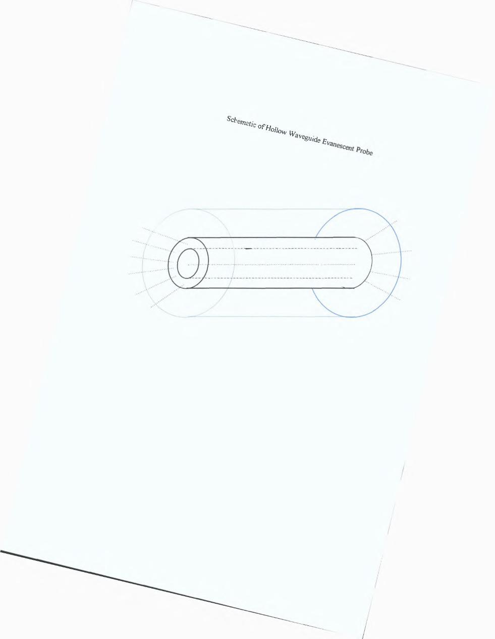
Schem tíl 0 f » o l,o w wVesui(je F
Eva»°scentp
Table of Contents
1 INTRODUCTION TO EVANESCENT WAVE SPECTROPHOTOMETRY 1
11 Modes in Waveguides 1
1 2 The Planar Waveguide 3
13 The Cylindrical Waveguide. 4
1 4 The Evanescent Power Fraction 7
1 5 The Waveguide as a Sensor 8
1 6 Absorbance of a Sensor Probe 9
1 7 Conclusions 10
1 8 References 11
2 THE HOLLOW CYLINDRICAL WAVEGUIDE - A THEORETICAL MODE ANALYSIS 12
2 1 Introduction 122J2 The £ and H fields of modes in a hollow waveguide 12
23 The mode eigenvalue equation 15
2 A Mode cut-off condition 18
2 5 Mode indices (I„ m) 20
2 6 Limiting values of 1 and m 222 7 The total number of bound modes 22
2 8 An effective V number for the waveguide (V') 232 9 The mode power in core and cladding 23
2 10 The evanescent power fraction of a mode 242 11 Conclusions 24
2 12 References 25
3 MODEL OF HOLLOW CYLINDRICAL WAVEGUIDES - A COMPUTATIONAL ANALYSIS 26
3 1 Introduction 26
3.2 Program to determine mode cut-off values 26
3 3 Computer program to solve the eigenvalue equation 29
3 4 Program to derive E and H field component amplitudes in core and cladding 29
3 5 Program to evaluate mean evanescent power fraction f among modes 30
3 6 Mode power fraction distribution 33
3 7 Dependence of f on V' and (b/a) 35
3 8 Dependence of N on V' 37
3 9 Conclusions 39
3 9 References 40
4 EVANESCENT WAVE SPECTROPHOTOMETRY USING A HOLLOW WAVEGUIDE PROBE 41
4 1 Inti oduction 41
4 2 The ATR probe 41
4.3 Excitation of modes in the probe 41
4 4 Theoretical absorbance of hollow waveguide probe 43
4.5 Absorbance measurement technique 45
4 6 Conclusions 47
5 EXPERIMENTAL ABSORBANCES USING HOLLOW SILICA WAVEGUIDE 48
5 1 Introduction 48
5 2 Bulk properties of the absorbing cladding 48
5.3 Evanescent absorbance as a function of probe immersion depth 495 4 The experimental f value 515 5 Conclusions 525 6 References 53
APPENDIX A CUTS M A-1
APPENDIX B CUTOUT M B-1
APPENDIX C HOLLM C-1
APPENDIX D HOLL_SEM D-1
APPENDIXE HOLLPOWM E-1
APPENDIX F MODESM F-1
APPENDIX G REFLECTION COEFFICIENT G-1
APPENDIX H 6X6 MATRIX H-1
Figure 1 1 The propagation constant $ o f a particular m ode ______________________ 1Figure 1 2 A Planar Waveguide _________________________________________Figure 1 3 Cylindrical Waveguide ______ _________________________________— — 4Figure 1-4 Power distribution in a waveguide ------------------_---------------- 9Figure 2-1 Hollow cylindrical w aveguide______________________________________ 12Figure 2-2 Radial E field o f (3, 3) mode __ .________________ 17Figure 2-3 Radial E fie ld in three dimensions _________________________________ „ 1 8Figure 2-4 Example o f I versus m graph ._______________________________________21Figure 3-1 Flow-chart o f program Cuts m ___________________________________ __ 21Figure 3-2 Flow-chart o f Holl m _____________________________________ ______.28Figure 3 3 Flow-chart fo r Holl_se m _________________________________________ _ 31Figure 3-4 Flow-chart fo r Hollpow m (continued in figure 3 -5 )________________________ 32Figure 3-5 Continuation o f flow-chart fo r Hollpow m ______________________________ 33Figure 3 6 Histogram o f power fraction f distribution ______________________________34Figure 3-7 f versus 1 /V t C = 1 5 ____________________________________________ 35Figure 3 8 f versus 1 /V, C = I 2 ____________________________________________ 36Figure 3-9 Graph o f f versus C _____________________________________________ 37Figure 3-10 C = 1 5 _____________________________________________________ 38Figure 3-11 C - 1 2 ____________________________________________________ 38Figure 4-1 Aluminum plug with fibers attached __________________________________ 42Figure 4-2 Light being focused into fiber bundle _________________________________ 43Figure 4-3 Example o f saturation o f absorbance with increasing depth __________________45Figure 5 I Bulk absorbance versus solution concentration __________________________ 49Figure 5 2 Evanescent absorbance versus depth (28 756yM solution) ___________________50Figure 5-3 Evanescent absorbance versus depth, (306 902\xM concentration) ______________ 51Figure G -l Reflection and transmission at an interface between two m e d ia_______________G-lFigure G-2 Light ray undergoing total internal reflection __________________________ G-2
Table 3-1 f values with corresponding mode percentages ___________________________ 34
Ta b l e o f F i g u r e s
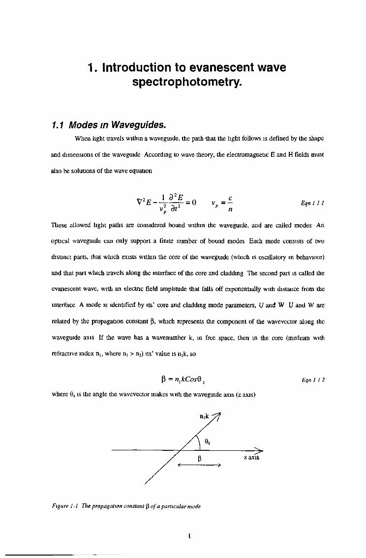
1. Introduction to evanescent wave spectrophotometry.
1.1 Modes in Waveguides.When light travels within a waveguide, the path that the light follows is defined by the shape
and dimensions of the waveguide According to wave theory, the electromagnetic E and H fields must
also be solutions of the wave equation
These allowed light paths are considered bound within the waveguide, and are called modes An
optical waveguide can only support a finite number of bound modes Each mode consists of two
distinct parts, that which exists within the core of the waveguide (which is oscillatory in behaviour)
and that part which travels along the interface of the core and cladding The second part is called the evanescent wave, with an electric field amplitude that falls off exponentially with distance from the
interface A mode is identified by its’ core and cladding mode parameters, U and W U and W are
related by the propagation constant (3, which represents the component of the wavevector along the
waveguide axis If the wave has a wavenumber k, in free space, then in the core (medium with
refractive index n1? where ni > n2) its’ value is n^, so
n
cEqn 111
P = n{kCosQ z Eqn 1 12
where 0Z is the angle the wavevector makes with the waveguide axis (z axis)
zaxis>
Figure 1-1 The propagation constant fi of a particular mode
1
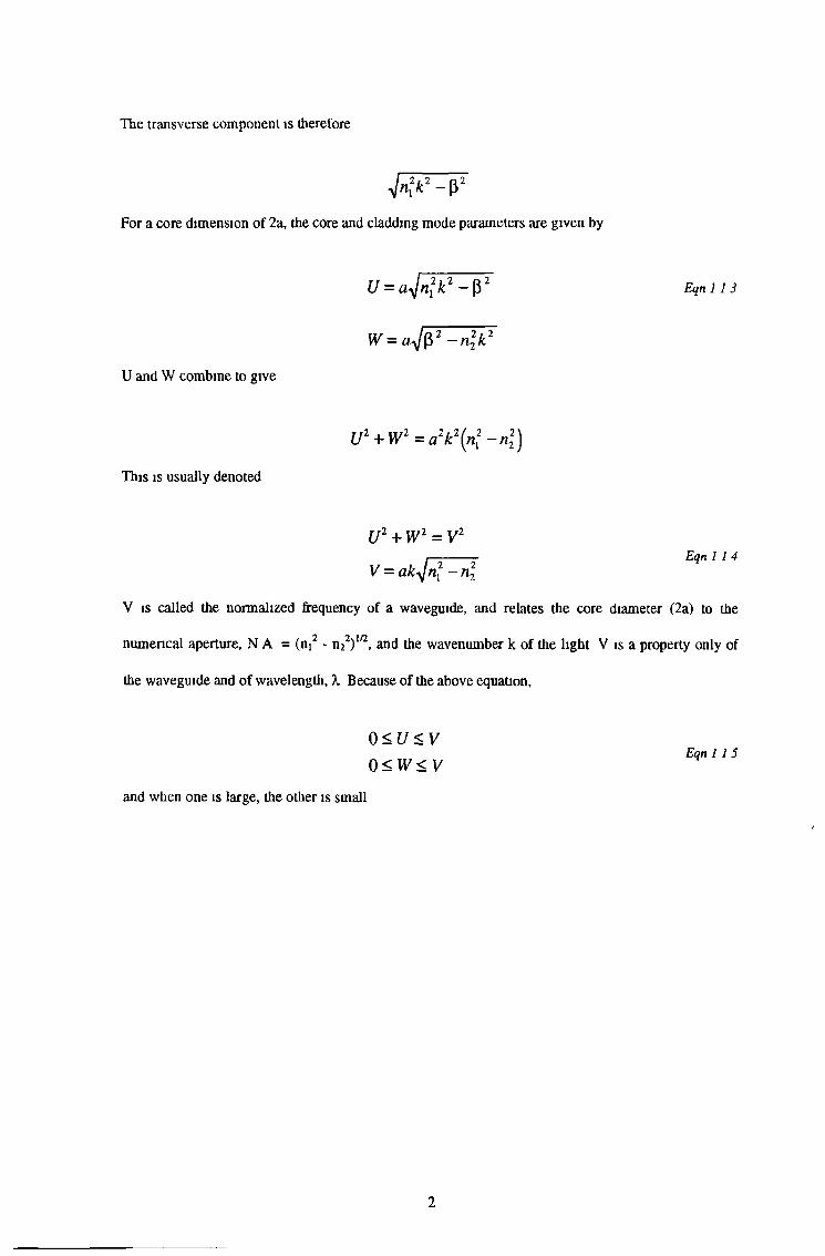
The transverse component is therefore
V«?*2 - p 2
For a core dimension of 2a, the core and cladding mode parameters are given by
U and W combine to give
U = a-Jnfk2 ~P Eqn I 1 3
W = a J $ 2 -n2V
U2 + W2= a 2k2(n f- n22)
This is usually denoted
Eqn 114u2 + w2 = V2
V = ak^Jnf —n\
V is called the normalized frequency of a waveguide, and relates the core diameter (2a) to the
numerical aperture, N A = (ni2 - n22)1/2, and the wavenumber k of the light V is a property only of
the waveguide and of wavelength, X Because of the above equation,
0 < U < VEqn 1150 < W < V
and when one is large, the other is small
2
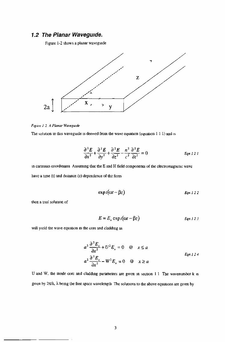
1.2 The Planar Waveguide.Figure 1-2 shows a planar waveguide
2a
Figure 1 2 A Planar Waveguide
The solution to this waveguide is derived from the wave equation (equation 111) and is
d2E d2E d2E n1 d2E+dx2 dy2 dt 2 dt2 = 0 Eqn 12 1
in cartesian coordinates Assuming that the E and H field components of the electromagnetic wave
have a time (t) and distance (z) dependence of the form
expi(aw - Pz)then a trial solution of
Eqn 1 2 2
E = EX exp/(co/-Pz) will yield the wave equation m the core and cladding as
Eqn 12 3
2 ^ E x dx2
a2^ - ^ - W 2Ex=0 @ x>adx
Eqn 1 2 4
U and W, the mode core and cladding parameters are given m section 1 1 The wavenumber k is
given by 2n/X, X being the free space wavelength The solutions to the above equations are given by
3
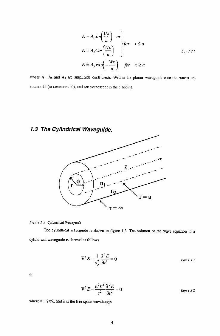
= AlSin{— ] \ a J
(— \ V a )
or
E = A2 C osfor x < a
Eqn 1 2 5
WxE = A3 exp — — j far x >a
where Ai, A2 and A3 are amplitude coefficients Within the planar waveguide core the waves are sinusoidal (or cosinusoidal), and are evanescent in the cladding
1.3 The Cylindrical Waveguide.
Figure 1 3 Cylindrical Waveguide
The cylindrical waveguide is shown m figure 1-3 The solution of the wave equation in a cylindrical waveguide is derived as follows
1 d2EV £ - ^ T f = 0 E9n l 3 lv. drP
„a n2k2d2Ec2 dt2 " ° Eqn132
where k = 2niXy and X is the free space wavelength
4
Expressing equation I 3 1 in cylindrical polar coordinates (r,<J) z) and inserting a trial solution of
E = E(r,<|>)exp j(coi - Pz) = Et exp i(coi - (iz)
gives
Eqnl 3 3
d Et 1 dE( 1 d E{ ( 2 2 2xl ^ +717+7 ‘ - p >£'=l)
Changing to a normalised radius R = r/a gives
d 2 E, 1 d E , 1 d 2E, 2 , 2 l 2 a U r , n— - J - + r~L+ , + a 2 ( n k - B IE, = 0 E q n l 3 5d R 2 R d R R 2 d (|>2 v H 1 ‘
Since the medium has cylindrical symmetry we can write
E , = F(R)<t>($) Eqn 13 6
i e separating E, in radial (R) and azimuthal (<J>) components Equation 13 5 then gives
R 2 \ d 2F 1 dF l „ 2 / 2 , 2 o2\ 1 d 2Q — r +-----> + R In k “ 3 ) = ------ r E q n l 3 7F [dR R d R J v H ’ O d § 2If we write equation 1 3 7 as some positive quantity + 12 then
1 d 2<t> ,2= I Eqn 1 3 8<t> ¿<(>2which has (S H M ) solutions of the form Cos or Sin Uj> For the function to be single valued, 1 e
4>(<|>) = <&(<(>+ 2rt) E q nl 3 9
we must have I = 0, 1, 2, 3 Since for each value of I there may be two independent states of
polarisation, modes with t > 1 are four fold degenerate while I = 0 modes, being independent are
two fold degenerate In equation 13 7 above the second term R2 (n2 k2 -p2) may be positive or
negative depending on the relative magnitude of nk and p
a) When n2tk2 > p2 > n22k2
5
For p in this range the radial fields F(R) are oscillatory in the core and decay in the cladding
(evanescent) These are known as guided modes or bound modes Recalling that p represents the z
component of the wavevector iiik in the core, Snell’s Law for rays says that guided or internally
reflected rays occur if
0 > Sin~l —ni
nx SinQ > n2 Eqn 1310n{kSin& >n2k
Where 0 is the angle the ray makes with the normal at the interface Now 0 + 0Z = rc/2 therefore
Snell’s Law gives
nlkCosQz > n2k i e p > n2k
for total internal reflection Since p = nik Cos 0Z, pmaJi is n^ so we have
Eqn I 3 11
nìk> p > n2k Eqn 13 12
for total internal reflection (0Z is shown in Figure 1-1 )
b) pz < n22k2
For such values of p the radial fields F(R) are oscillatory in the cladding These are known as
radiation modes and correspond to refracted light in the cladding
Returning to equation 13 7 the wave equation for guided or bound modes becomes
r2^ + R^ + (u 2r2-i2)f = 0 R<1dR dRR 2^ - + R ^ r - ( w 2R 2 + i 2)f = o r > idR2 dR v '
, Eqn 13 13d F „ dF
where
U1 = a 2(n2k 2 - p 2)
W 2 = a 2( ^ 2 - n 2k 2)Eqn 1 3 14
6
Equations 1 3 13 are of the standard form of Bessel Equations with solution J{ (UR), Y, (UR) m the R <
1 core region and modified Bessel functions K^(WR) and I* (UR) in the cladding
The equations above give the allowed solutions
where A t is the wave amplitude The Yt(UR) and I|(UR) Bessel functions are not allowed solutions in
this case as Y, (UR) is infinite at R = 0, and I( (UR) is infinite at R = 1 (Abramowitz and Stegun,
Figures 9 1 and 9 8)
1.4 The Evanescent Power Fraction.For both planar and cylindrical waveguides the evanescent field
(i) is approximately exponentially decaying away from the interface
(11) Has a penetration depth = a/W, or
evanescent wave may be calculated Thus the power fraction of a mode which exists as an evanescent wave can be determined This fraction f, was shown by Gloge (1971) to be
E, = A, J,(UR)Cos(l$) | >for R< 1
or E, = A, Jl{UR)Sin(l§)E^^KXW QCosQ ï) 1_ Jfor R> 1 or El= A lK,(WR)Sin(l4>)
Eqn 1 3 15
By taking the Poyntmg vector ( E x H ) and integrating from R = 1 to R = the power of the
u 2Eqn 14 1
\
1
For modes dose to cut-off, 1 e modes for which W 0, this fraction will be large, (W -» 0 as U ->
V)
f=Yi
while for modes far from cutolf (W -> V, as U 0) the power fraction will be negligible
1.5 The Waveguide as a Sensor.In order for a waveguide to be used as a sensor, an analytical wavelength of the cladding
material must match that of the light being carried by the core The cladding will then absorb photons
from the modes at a rate determined by the bulk absorption coefficient of the cladding material (which
may be solid or fluid) The amount of absorption that occurs also depends on the distance over which
the core is in contact with the absorbing medium The sensing mechanism is the detection of the size
of this power loss into the absorber, and relating the power loss to the concentration of absorber
present Various evanescent wave sensor geometries are possible Hamck (1987) Chapter 4 discusses
rectangular waveguide designs Kapany et al (1963) I and II, Hansen (1963) and Hamck (1964)
describe solid rod waveguides used m attenuated wave spectrophotometry
8
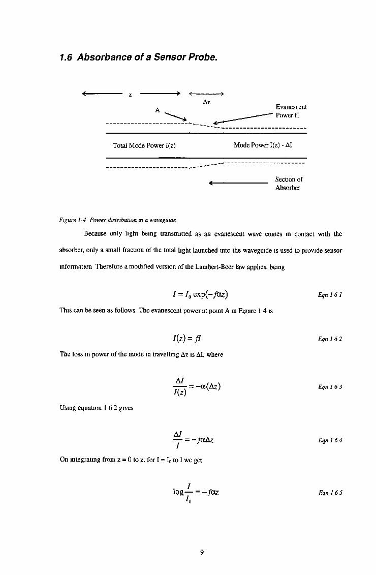
1.6 Absorbance of a Sensor Probe.
Total Mode Power I(z) Mode Power I(z) - AI
Section of Absorber
Figure 1-4 Power distribution in a waveguide
Because only light being transmitted as an evanescent wave comes in contact with the
absorber, only a small fraction of the total light launched into the waveguide is used to provide sensor
information Therefore a modified version of the Lambert-Beer law applies, being
I = I 0 e x p ( - /a z ) E q n l 6 1
This can be seen as follows The evanescent power at pomt A m Figure 1 4 is
/ (z ) = f l E q n l 6 2
The loss in power of the mode in travelling Az is AI, where
61 /A %— = - a (A Z) Eqnl 6 3I{z)Using equation 16 2 gives
AI— = - f a A z E q n l 6 4
On integrating from z = 0 to z, for I = I0 to I we get
lo g — = - f t X Z E q n l 6 5h
9
i e
/ = /„ ex p (- a fz) Eqn 166
A ' = (0 434) fctz Eqn 167
For a given mode, specified by the core mode parameter U, and cladding mode parameter W, then the
above equation gives the evanescent absorbance A' using equation 1 4 1 for f - as
A ' = (0 43 4 ) U 2azEqn 16 8
v2Jw2+i2 + 1In this case z is the length of the waveguide in contact with the absorber Where many modes are
excited, each with the same incident power (I0 / N), the transmitted power will be
V 2-JW2+ l2+ l
Yu
A ' = - log 10 r r l exp-azU
N r [yfiF+r+i
where tlie summation is earned out over N modes A' is the evanescent absorbance
Eqn 16 9
Eqn 1 6 10
Eqn 1 6 11
1.7 Conclusions.This chapter provides the basis from which theoretical analysis on the hollow cylindncal
waveguide will be done The methods shown above will be expanded to desenbe the hollow
waveguide in similar mathematical terms, so that the hollow waveguide will desenbe both the planar
and fibre waveguides when the dimensions of the hollow waveguide are sufficiently large to be
considered planar or small enough to be considered a solid fibre
;
10
1.8 References.Abramowitz M and Stegun I A, “Handbook of Mathematical Functions”, (National Bureau oi
Standards, Washington DC USA 1964) Eqn 9-5-28 p374
Gloge D, “Weakly Guiding Fibers”, Appl Opt 10 pp 2252 - 2258 (1971)
Hansen W N, “A New Spectrophotometnc Technique using Multiple Attenuated Total Reflection”,
Anal Chem 35 765-769(1963)
Harrick N J, “Multiple Reflection Cells for Internal Reflection Spectroscopy”, Anal Chem 36 188-
193 (1964)
Harrick N J, “Internal Reflection Spectroscopy”, (Hamck Scientific Corp NY (1987))
Kapany N S and Pontarelli D A (I), “Photorefractometer I Extension of Sensitivity and Range”,
Appl Opt 2 425-430(1963)
Kapany N S and Pontarelli D A (II), “Measurement of N and K’\ Appl Opt 2 1043-1050 (1963)
Snyder A W and Love J D,“Optical Waveguide Theory”, (Chapman and Hall, London / NY (1983))
11
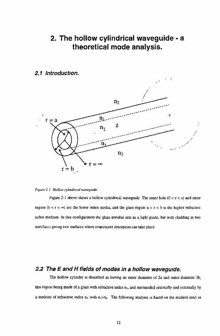
2. The hollow cylindrical waveguide - a theoretical mode analysis.
2.1 Introduction.
//
Figure 2 1 Hollow cylindrical waveguide
Figure 2-1 above shows a hollow cylindrical waveguide The inner hole (0 < r < a) and outer
region (b < r < °o) are the lower index media, and the glass region a < r < b is the higher refractive
index medium In this configuration the glass annulus acts as a light guide, but with cladding at two
interfaces giving two surfaces where evanescent absorption can take place
2.2 The E and H fields of modes in a hollow waveguide.The hollow cylinder is described as having an inner diameter of 2a and outer diameter 2b,
this region being made of a glass with refractive index ni, and surrounded internally and externally by
a medium of refractive index n2 with ni>n2 The following analysis is based on the method used in
12
Unger(1980) for E and H fields in doubly clad cylindrical fibre waveguides modified for the hollow
cylinder
Barlow (1981, 1983) developed the first published work on the “three concentric layer
cylindrical waveguide” In his analysis - pertaining to fiber waveguides - the waveguide dimensions
are small (typically 100 pm) and the refractive indices of the 3 layers (n, n2, n3) are very close
together, obeying the so-called “weakly guiding approximation” The latter condition is valid only in
very limited cases but the thrust of the mode analysis can form a basis for a more general theory Tsao
et al (1989) earned out further 3 layer fiber mode characterisations, again invoking a weakly guiding
condition Brunner et al (1995) published some work on Attenuated Total Reflection
Spectrophotometry using “capillary optical fiber” probes using the mode analysis technique of Barlow
(1983) for their work Mode analysis for a 3 layered cylindrical waveguide of a hollow cylinder shape, where the guiding glass annulus is surrounded by 2 media of the same refractive index (as shown in
figure 2 1) is carried out by the author without recourse to the weakly guiding condition (ni = n2)
This is the most general case and the analysis described here is the first representation of such a treatment
Solutions of the wave equations in a medium m which the phase velocity of light is x> = c/n
(where V2 is a vector operator) may be expressed in terms of the two waveguide parameters U and W, defined in equation 113 The two vector differentials 2 2 1 for E and H can be broken into six differential scalar equations Of these, four mvolve more than one E of H field component The other two involve the z components Ez or Hz alone These can be wntten as
Eqn 2 21
13
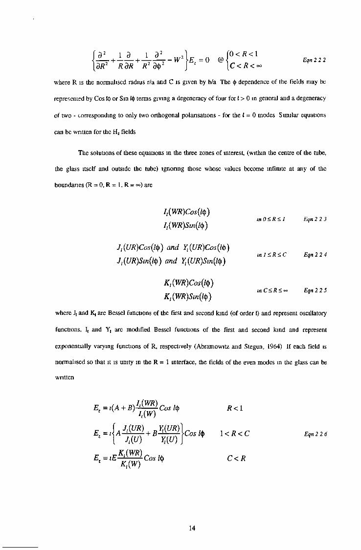
- w 2 \ e z = 0 @0 < R < 1
C < R < ° ° Eqn 2 2 2
where R is the normalised radius r/a and C is given by b/a The § dependence of the fields may be
represented by Cos i<() or Sm i<|) terms giving a degeneracy of four for (> 0 in general and a degeneracy
of two - corresponding to only two orthogonal polarisations - for the I = 0 modes Similar equations
can be written for the Hz fields
The solutions of these equations m the three zones of interest, (within the centre of the tube,
the glass itself and outside the tube) ignoring those whose values become infinite at any of the
boundaries (R = 0, R = 1, R = °o) are
where J{ and K, are Bessel functions of the first and second kind (of order () and represent oscillatory
functions, I< and Y{ are modified Bessel functions of the first and second kind and represent
exponentially varying functions of R, respectively (Abramowitz and Stegun, 1964) If each field is
normalised so that it is unity in the R = 1 interface, the fields of the even modes in the glass can be written
I,(WR)Cos(h|>)
II{WR)Sin(h)>)in 0<R< 1 Eqn 2 2 3
7,(W?)Cas(/(t)) and Y, (UR)Cos(bS}) J,{UR)Sin(l<b) and Yt (UR)Sin(l<\)) in 1 <.R<,C Eqn 2 2 4
K,(WR)Cos(l<Sf) Kl{WR)Sin(l^) in C < R < Eqn 22 5
R< 1
1 < R < C Eqn 226
C < R
14
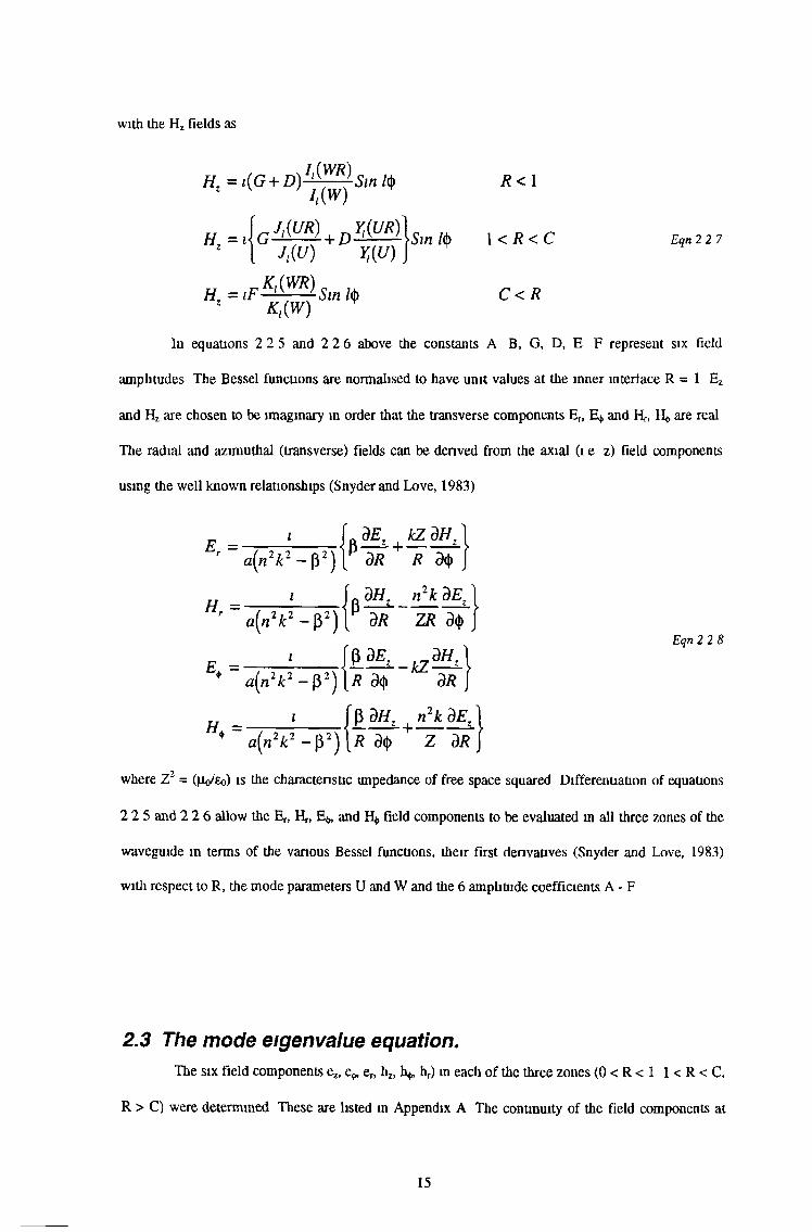
with the H z fields as
H. = i[G + Ü)-^-— Sin /(|) * v ' It{W)
R< 1
1< R < C Eqn 227
C < R
In equations 22 5 and 22 6 above the constants A B, Gt D, E F represent six field
amplitudes The Bessel functions are normalised to have unit values at the inner interface R = 1 Ez
and Hz are chosen to be imaginary in order that the transverse components Er, E0 and H, are real
The radial and azimuthal (transverse) fields can be derived from the axial (i e z) field components
using the well known relationships (Snyder and Love, 1983)
2 2 5 and 2 2 6 allow the Er, and H* field components to be evaluated in all three zones of the
waveguide in terms of the various Bessel functions, their first derivatives (Snyder and Love, 1983) with respect to R, the mode parameters U and W and the 6 amplitude coefficients A - F
2.3 The mode eigenvalue equation.The six field components ez, e ef, hz, h^ hr) in each of the three zones (0<R<1 1<R<C,
R > C) were determined These are listed in Appendix A The continuity of the field components at
Eqn 2 2 8
where Z2 = Qio/Eo) is the characteristic impedance of free space squared Differentiation of equations
15
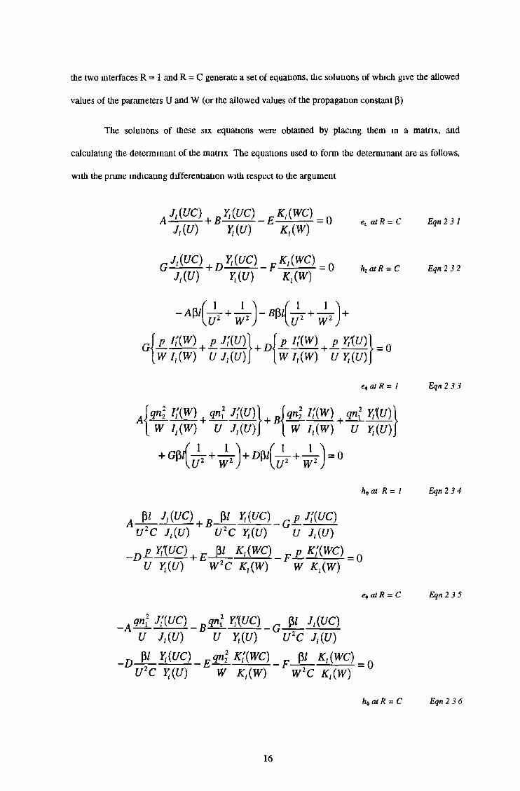
the two interfaces R = 1 and R = C generate a set of equations, the solutions of which give the allowed
values of the parameters U and W (or the allowed values of the propagation constant ¡3)
The solutions of these six equations were obtained by placing them in a matrix, and
calculating the determinant of the matrix The equations used to form the determinant are as follows,
with the prime indicating differentiation with respect to the argument
J,(UC) , ^ ( U C ) e K ,(W C )_J,(U) Y,(U) K ,(W )
ez at R = C Eqn 2 31
C J,(UC) , d Y,(UC) r K , (W C )_ QJ,(U) Yt(U) K,{W) hz at R = C Eqn 2 3 2
e$ at R = 1 Eqn 2 3 3
gn\ i;(W) | gn\ Yt'{U) W I,(W) U Y,(U)
h$at R = / Eqn 2 3 4
A fa j , (u c ) , B p/ Yt{uc) c p j;(uc)U2C J,{U) U2C Y,(U) U J,(U)
D P m o , E pi K,(WC) p k ; ( w c )U Y,(U) W 2C K,(W) W Kt(W)
e+atR = C Eqn 2 3 5
A qnl j;{UC) D gn2 Y({UC) g pI J,(UC)U J t(U) U Y,(U) U 2C J,(U)
D P/ Y,(UC) _ E gn\ K!(WC) _ pI K,(WC) =U 2C Y,(U) W K,(W) W 2C K,(W)
at R = C Eqn 2 36
16
Each pair of U and W values (same p value) that allow the value of the determinant to be
zero (for a range ot I values) is considered to be a valid solution, and therefore an allowed mode,
provided it also meets the cut-off condition (which is discussed in section 2 4)
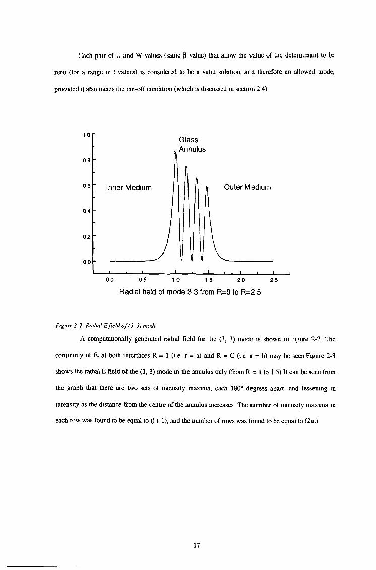
Radial field of mode 3 3 from R=0 to R=2 5
Figure 2-2 Radial E field of (3, 3) mode
A computationally generated radial field for the (3, 3) mode is shown in figure 2-2 The
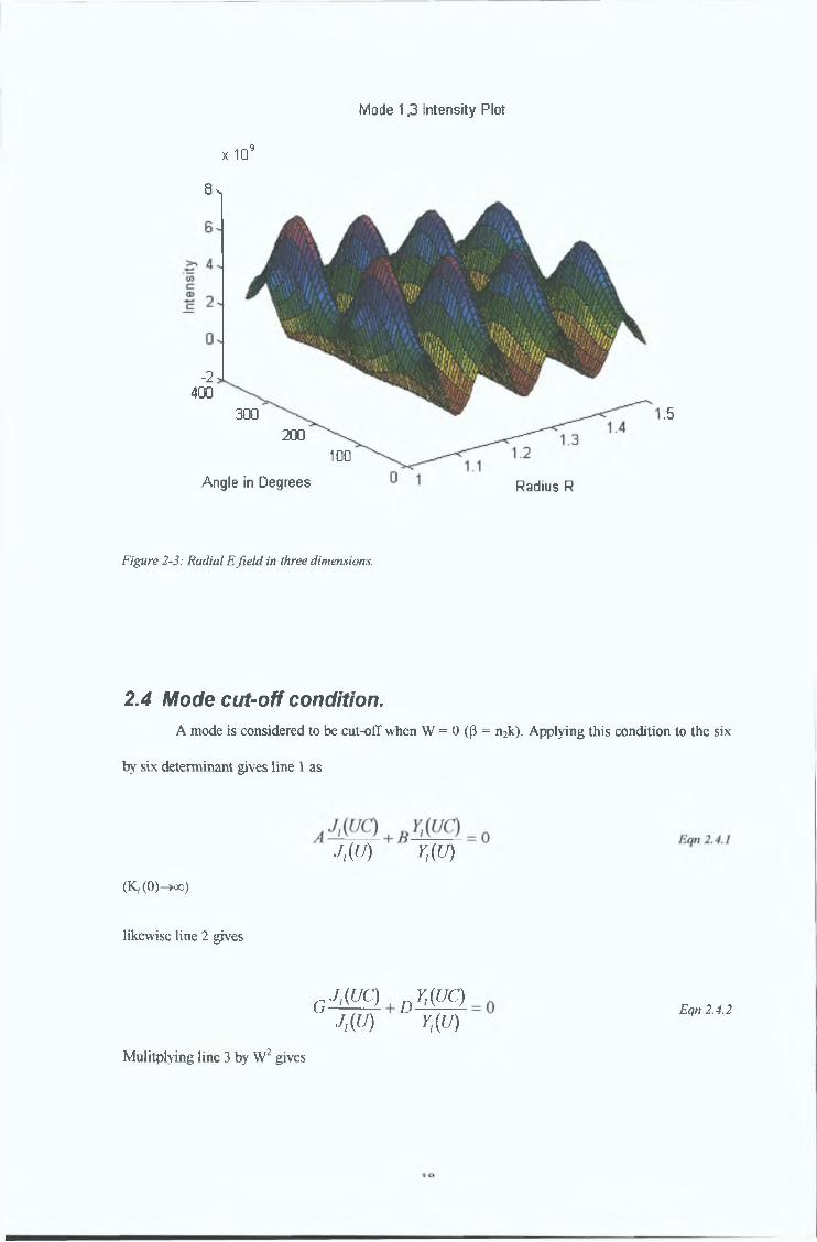
continuity of E, at both interfaces R = 1 (i e r = a) and R = C (i e r = b) may be seen Figure 2-3
shows the radial E field of the (1, 3) mode in the annulus only (from R = 1 to 1 5) It can be seen from
the graph that there are two sets of intensity maxima, each 180° degrees apart, and lessening in
intensity as the distance from the centre of the annulus increases The number of intensity maxima ineach row was found to be equal to (i + 1), and the number of rows was found to be equal to (2m)
17
Mode 1,3 Intensity Plot
X 109
8 V
.5
Figure 2-3: Radial E field in three dimensions.
2.4 Mode cut-off condition.A mode is considered to be cut-off when W = 0 (P = n2k). Applying this condition to the six
by six determinant gives line 1 as
J,(U) r,(u)
(Kf (0)—*»)
likewise line 2 gives
c J , m . rj,(uc)m r,(u)
Eqn 2.4.2
-2 400
300200
100Angle in Degrees Radius R
Mulitplying line 3 by W 2 gives
Similarly line 4 by W 2 gives
- p M - p / f l = 0
=> A + £ = 0Eqn 2 4 3
P /G + P / D = 0
=> G + D = 0
Mulitplying line 5 by W 2 gives
And line 6 by W gives
Eqn 24 4
Eqn 24 5
F = 0
The solution of equations 2 4 land 2 4 3 give the cut-off conditionEqn 2 4 6
J t{VC) Yt{UC)
Ji(U) Yt{U)1 1
= 0Eqn 2 47
or J l (UC)Yl (U ) -Y l(U C)Jl {U) = 0
For each integer value of t (0, 1, 2 ) the above equation has many roots, which are specified by m =
1, 2, 3 Thus an array of U values indexed by (and m (Ut m) mode can be created
Each member of the family of (Ut m)cut-off values is the lowest possible value for a solution to
the six by six determinant for its’ given (t, m) values
Vim > ( * 0tm \ I m J cut- 0ff Eqn 2 4 8
Since the maximum value of U is V (the V number of the waveguide) at which W = 0, the cut-off condition for the (i, m) mode becomes
J l(VC)Yl(V )-Y l(VC)J,(V) = 0 Eqn2 4 9
Soluuons to the above equation are given in Abramowitz and Stegun (1964), equation 9-5-28, page
374 as
Eqn 2 4 10
19
where (3 = mre/C -1
\l = 4i2
p = (U- 1)/8C
q = (H -1) (H - 25) (C3 - 1) / 384C3 (C -1)
r = (n -1) (n2 - 114(1+ 1073) (C5 -1) / 5120C5 (C -1)
(p above is not the propagation constant defined earlier in equation 112)I
Equation 2 4 10 is valid only for p » p / p or
For the fundamental mode (i - 0, m = 1) single mode operation exists for V = 12 6 with C =
1 25 and for V = 6 27 with C = 15(V<rc/(C-l) approximately) Equation 2 4 10 can be used to
extract the maximum value of m for (= 0 modes and yields the value
Expanding equation 2 4 10 to the second term yields a functional relationship between I and m of
where E, F and G are functions of V and C (E = 4, F = 8rcCV and G = 8tc*C / (C - 1)) For a large V
number waveguide (V » > 1) the third term in equation 2 5 2 can be disregarded so that
i f C - lm » P ----^2k C* j
Eqn 2 4 11
2.5 Mode indices (fm).
Eqn 2 51
El2 + Fm+Gm2 = 0 Eqn 2 5 2
El2 + Fm = 0
i e (and m are related in a parabolic fashion forEqn 2 5 3
20
m2
» P( C-l Eqn 2 5 42 rcC3
For the other extreme, i e small m and large I the approximation of equation 2 4 10 no longer holds
Numerical modelling indicates that an equation of the form
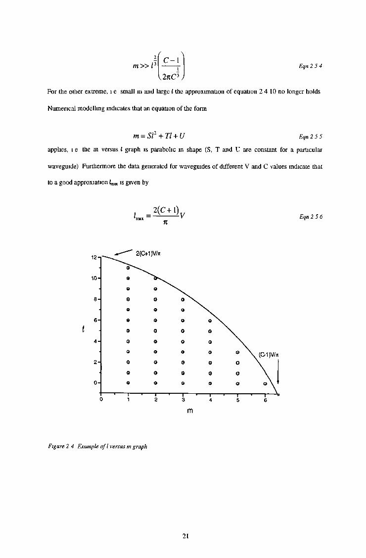
tn = SI2 + TI + U Eqn 255
applies, i e the m versus I graph is parabolic in shape (S, T and U are constant for a particular
waveguide) Furthermore the data generated for waveguides of different V and C values indicate that
to a good approxiaUon is given by
2(C +1)Eqn 2 5 6
Figure 2 4 Example of I versus m graph
21
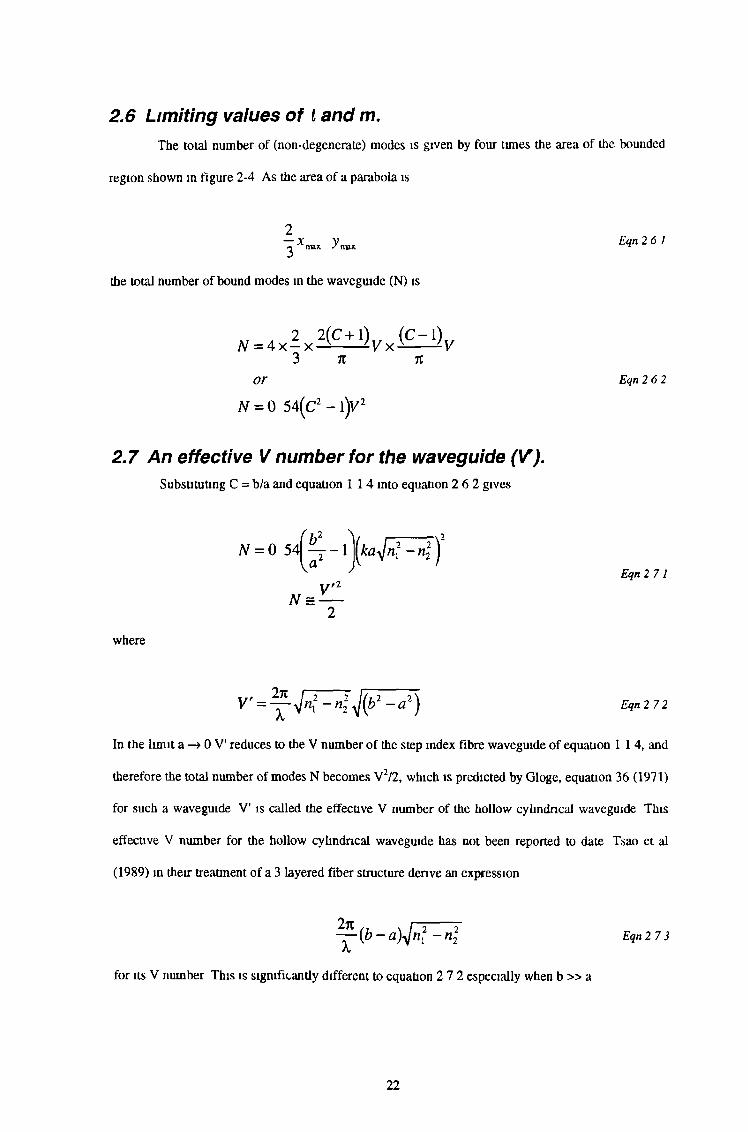
2.6 Limiting values of I and m.The total number of (non-degenerate) modes is given by four times the area of the bounded
region shown m figure 2-4 As the area of a parabola is
22* ™ , Eqn2 6I
the total number of bound modes m the waveguide (N) is
„ , 2 2 ( C + 1) ( C - l ) „N = 4 x — X — -V X - -V3 n %or Eqrt 26 2
N = 0 54(C2 -1 )V 2
2.7 An effective V number for the waveguide (V).Substituting C = b/a and equation 114 into equation 2 6 2 gives
V'2 N = —
2
Eqn 2 71
where
V' = y --y /« !2 - « 2 yj{b2 ~ ° 2) £?n 272
In the limit a->0V' reduces to the V number of the step index fibre waveguide of equation 114, and
therefore the total number of modes N becomes V2/2, which is predicted by Gloge, equation 36 (1971) for such a waveguide Vr is called the effective V number of the hollow cylindrical waveguide This
effecuve V number for the hollow cylindrical waveguide has not been reported to date Tsao et al (1989) in their treatment of a 3 layered fiber structure denve an expression
2n X
for its V number This is significantly different to equation 2 7 2 especially when b » a
22
2.8 Single mode operation.The condition for m max given m equation 2 5 1 may be used to derive the condiuon for single
mode operation of this waveguide Putting m max = 1 yields
(C-l)V<7t
{ b - d ) <
or\a )
TZ Eqn 2 81
(b-a)<
{k)NA
X2NA
i e if the waveguide thickness (b - a) is less than the light wavelength divided by twice the waveguide
numerical aperture NA [NA2 = n2 -n22], only the fundamental (0, 1) mode can propagate in the
waveguide This condition is quoted by Tsao et al (1989) for single mode operation of what they refer
to as a "Ring fibre waveguide" [Equation 9 123 of Tsao 1989] This is referenced m Tsao (1992)
which treats the three layered cylindrical waveguide using Debye potentials The field functions (Er,
E^ Ez) and (Hr, Hz) obtained by Tsao (1992) are identical to those quoted in this analysis when his
third layer refractive index n3 is equated to n2 m this analysis The author was not aware of this paper
when the enclosed analysis was carried out
2.9 The evanescent power fraction of a mode.The mode power m the z direction in all three zones in the waveguide may be obtained from
the Poynting vector
P: = m 2j ( E rH t - E ^ H r ] R d R Eqn 2 9 i
using the limits appropriate to the zone m question, i e (0, 1), (1, C) and (C, <*>) for the inner
cladding the core and the outer cladding, with the integration being made over the cross-sectional
23
area (The radial and azimuthal fields are given previously in equation 2 2 8) As the power ratios in
the evanescent fields only are of interest, the factor of 2n and
C o S 1 ( l § ) d § = TZ E q n 2 9 2
are ignored
2.10 The evanescent power fraction of a mode.The evanescent power fraction of each mode within a waveguide may be calculated from
l>r + i > rf t = ----------- ° C------- E q n 2 1 0 1
using equation 2 9 1 to evaluate Pz Summing over t and m for all allowed modes within a waveguide,
and dividing by the number of modes gives the average evanescent power fraction for a mode within a
particular waveguide
2.11 Conclusions.The above analysis shows that a hollow cylindrical waveguide can act as a light guide when
that light travels in the allowed modes dictated by the eigenvalue equations and the boundary conditions The core and cladding parameters U and W can be predicted for a waveguide of any given dimension for the equations discussed The number of modes that can be sustained by the waveguide
can also be predicted using the above theoretical derivations The power distribution of core guided
light to evanescendy bound light can also be described for each mode in the hollow cylindrical
waveguide
24
2.12 References.
Barlow H M, “A Large Diameter Optical Fiber Waveguide For Exclusive Transmission In The HEu
Mode”, J Phys D Appl Phys 16 1539-1451 (1983)
Barlow H M, “A Cladded Tubular Glass-fiber Guide For Singlemode Transmission” J Phys D
Appl Phys 14 405-412(1981)
Brunner R, Doupouec J, Suchy F and Berta M, “Evanescent -wave Penetration Depth in Capillary
Optical Fibers Challenges For The Liquid Sensing”, Acta Physica Slovaca 45 (4) 491-498 (1995)
Gloge D, “Weakly Guiding Fibres”, Applied Optics 10 pp2252 - 2258 (1971) Eqn 36
Snyder A W and Love J D “Optical Waveguide Theory”, (Chapman & Hall (1983)) Eqn 30-9 p593
Tsao C, “Optical Fibre Waveguide Analysis”, (Oxford University Press, NY (1992)), Section 9 2 pp 300 - 352
Tsao C Y H, Payne D N and Gambling W A, “Modal characteristics of three layered optical fibre waveguides a modified approach”, J Opt Soc Am A, pp 555-563 (1989)
Tsao C YH, Payne D N and Gambling W A, “Modal Characteristics of Three-Layered Optical Fiber Waveguides A Modified Approach”, J Opt Soc Am A 64, 555-563 (1989)
Unger H G, “Planar Optical Waveguides and Fibres”, (Clarendon Press, Oxford (1980))
25
3. Model of hollow cylindrical waveguides - a
computational analysis.
3.1 Introduction.
This chapter describes the computational methods and computer programs used to create an
accurate simulation of the bound modes in a hollow cylindrical waveguide probe Each of the
programs used was written m the Matlab language (which is based on matrices), and runs only in the
Matlab environment A program called Modes m was written to control the other programmes
3.2 Program to determine mode cut-off values.
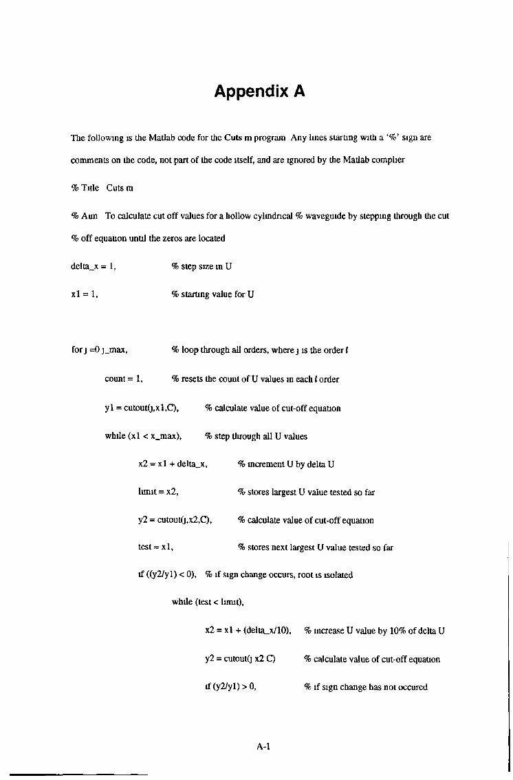
The following flow-chart (figure 3 1) describes the construction of the program used to
calculate the cut-off values for a given waveguide The main program is called Cuts m, and the
program which evaluates the cut-off condition at a particular U, I and C is called Cutout m The
cut-off condition in matrix form is given previously in equation 2 4 7 Any value of U the core mode
parameter, which allows the value of the cut-off condition to be zero is considered to be a cut-off value
for a particular t and m (the mode indices) It can be seen from equation 2 4 7 that the only other
parameter in the equation is the C (= b/a) value This means that there is only one set of cut-off values for any C, regardless of the actual dimensions of the waveguide This set of cut-off values is the output
of Cuts m, and is saved m matrix form The code for both of these programs is given in Appendices A and B
26
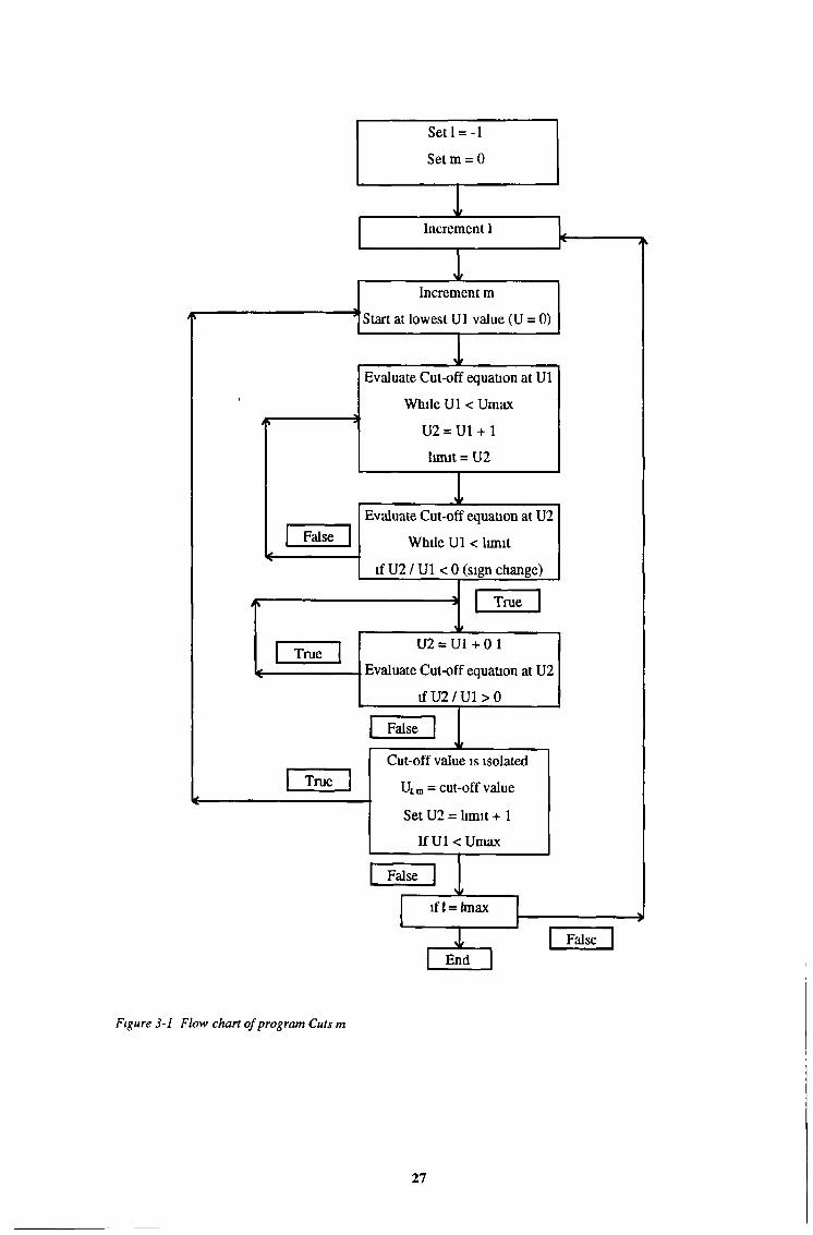
Figure 3-1 Flow chart of program Cuts m
27
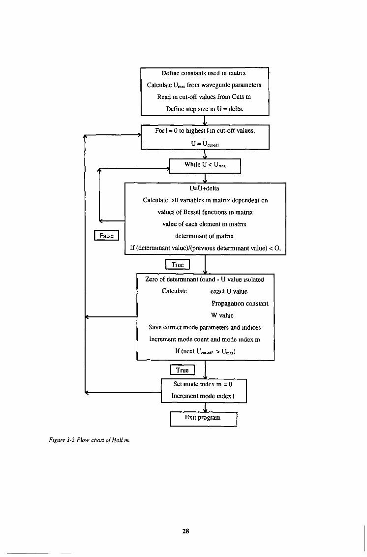
Figure 3-2 Flow chart of Holt m.
28
3.3 Computer program to solve the eigenvalue equation.
This program was called Holl m, the code is listed m Appendix C The purpose ot tins
program is to calculate the allowed U values in the hollow cylindrical waveguide based on the variable
parameters entered by the user To to this, the six eigenvalue equations of equations 2 3 1 to 2 3 6
were placed in a matrix form The determinant of the matrix was then calculated Each value of U
(with a particular I and m) for which the determinant of the matrix equalled zero was considered to be
a bound mode within the waveguide, provided the U value was greater then the appropriate cut-off
value for its' given mode indices (t and m) An incremental substitution method was used to find the
correct U values, with the starting U value being the correct cut-off value, so that this condition was
fullfilled automatically The flow-chart in figure 3-2 shows the logic steps used m Holl m, the code is
given in Appendix C
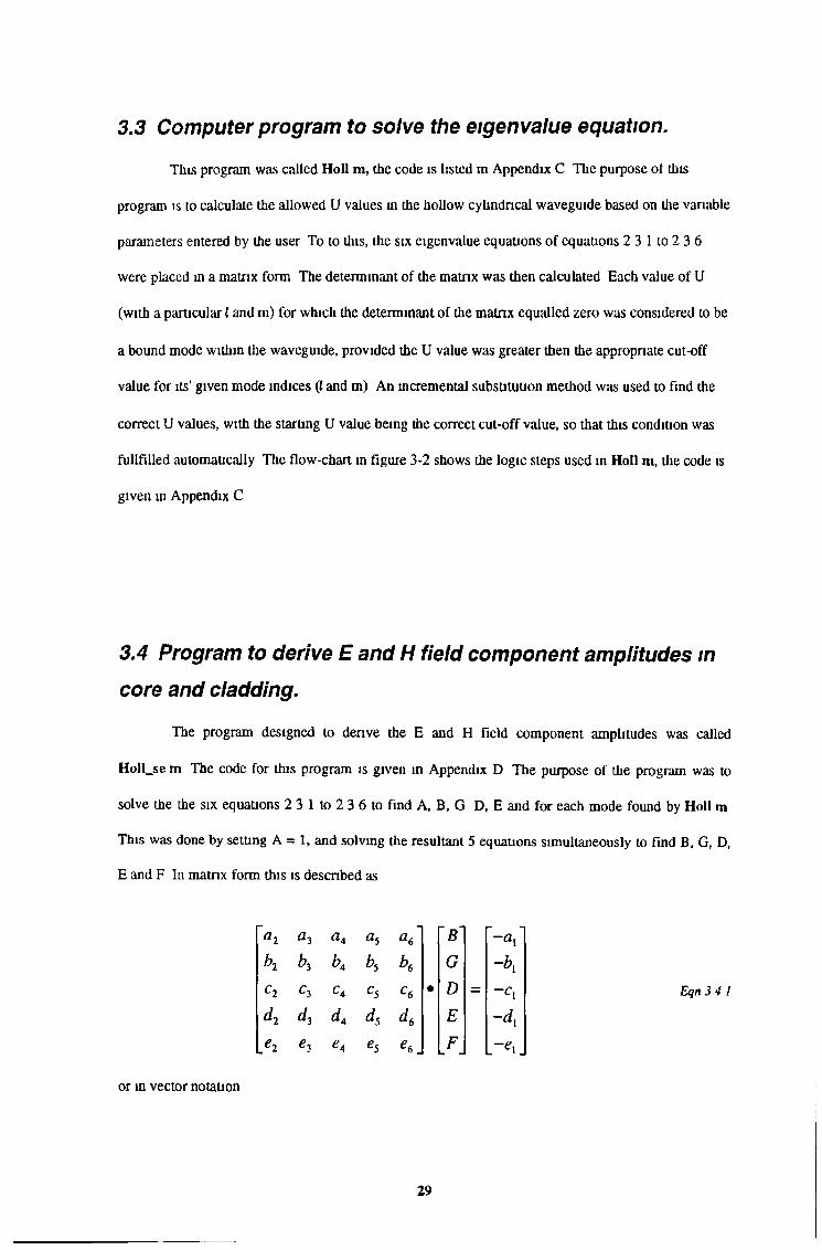
3.4 Program to derive E and H field component amplitudes in
core and cladding.
The program designed to denve the E and H field component amplitudes was called
Holl_se m The code for this program is given in Appendix D The purpose of the program was to
solve the the six equations 231to236 to find A, B, G D, E and for each mode found by Holl m This was done by setting A = 1, and solving the resultant 5 equations simultaneously to find B, G, D, E and F In matrix form this is described as
~a2 a 3 « 4 « 5 a 6 B ~ a \
b2 h K h b6 G -b{
C2 C4 Cs • D =d2 d3 d> ds d6 E -d\J 2 *3 e 4 «5 e6. F r e i .
or in vector notation
29
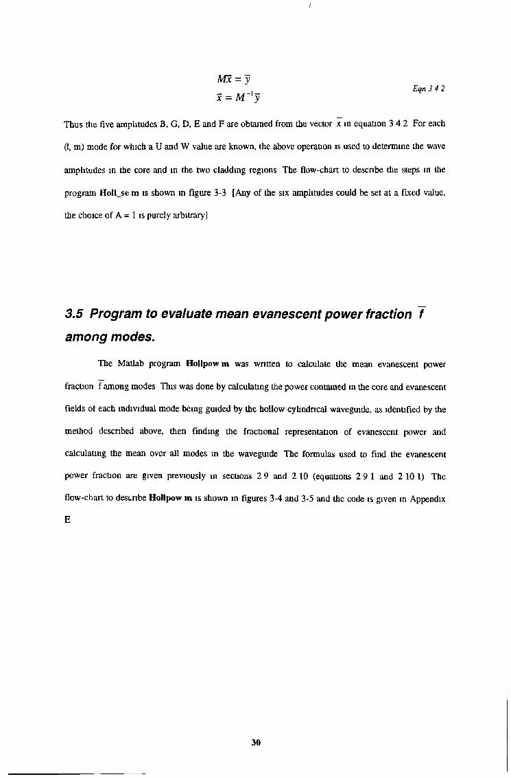
Mx = yX = M~'y
Thus the five amplitudes B, G, D, E and F are obtained from the vector x in equation 3 4 2 For each
(i, m) mode for which a U and W value are known, the above operation is used to determine the wave
amplitudes in the core and m the two cladding regions The flow-chart to describe the steps in the
program HoIl_se m is shown in figure 3-3 [Any of the six amplitudes could be set at a fixed value,
the choice of A = 1 is purely arbitrary]
Eqn 3 4 2
3.5 Program to evaluate mean evanescent power fraction f
among modes.
The Matlab program Hollpowm was written to calculate the mean evanescent power
fraction f among modes This was done by calculating the power contained in the core and evanescent
fields ot each individual mode being guided by the hollow cylindrical waveguide, as identified by the
method described above, then finding the fractional representation of evanescent power and
calculating the mean over all modes in the waveguide The formulas used to find the evanescent
power fraction are given previously in sections 2 9 and 2 10 (equations 2 9 1 and 2 10 1) The
flow-chart to describe Hollpow m is shown in figures 3-4 and 3-5 and the code is given in Appendix E
30
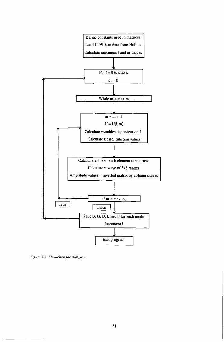
Figure 3-3 Flow-chart for Holljse m
31
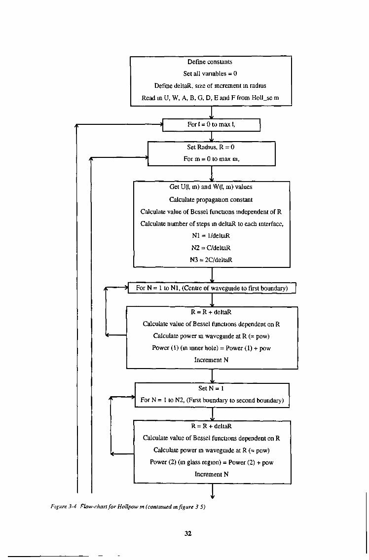
Define constants Set all variables = 0
Define deltaR, size of increment m radius Read in U, W, A, B, G, D, E and F from Holl_se m
For ( = 0 to max I,w
Set Radius, R = 0 For m = 0 to max m,
Get U(i, m) and W(f, m) values Calculate propagation constant
Calculate value of Bessel functions independent of R Calculate number of steps m deltaR to each interface,
N1 = 1/deltaR N2 = C/deltaR N3 = 2C/deltaR
1tFor N - 1 to Nl, (Centre of waveguide to first boundary)
*R = R + deltaR
Calculate value of Bessel functions dependent on R Calculate power in waveguide at R (= pow) Power (1) (in inner hole) = Power (1) + pow
Increment N
it___Set N = 1
For N = I to N2, (First boundary to second boundary)
R = R + deltaR Calculate value of Bessel functions dependent on R
Calculate power in waveguide at R (= pow) Power (2) (in glass region) = Power (2) + pow
Increment N
IFigure 3-4 Flow-chart for Hollpow m (continued in figure 3 5)
32
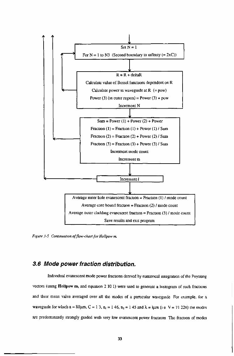
Figure 3-5 Continuation offlow-chart for Hollpow m.
3.6 Mode power fraction distribution.
Individual evanescent mode power fractions derived by numerical integration of the Poynting
vectors (using Hollpow m, and equation 2 10 1) were used to generate a histogram of such fractions
and their mean value averaged over all the modes of a particular waveguide For example, for a
waveguide for which a = 80pm, C = 1 3, n, = 1 46, n2 = 1 45 and X = lpn (l e V= 71 226) the modes
are predominantly strongly guided with very low evanescent power fractions The fraction of modes
33
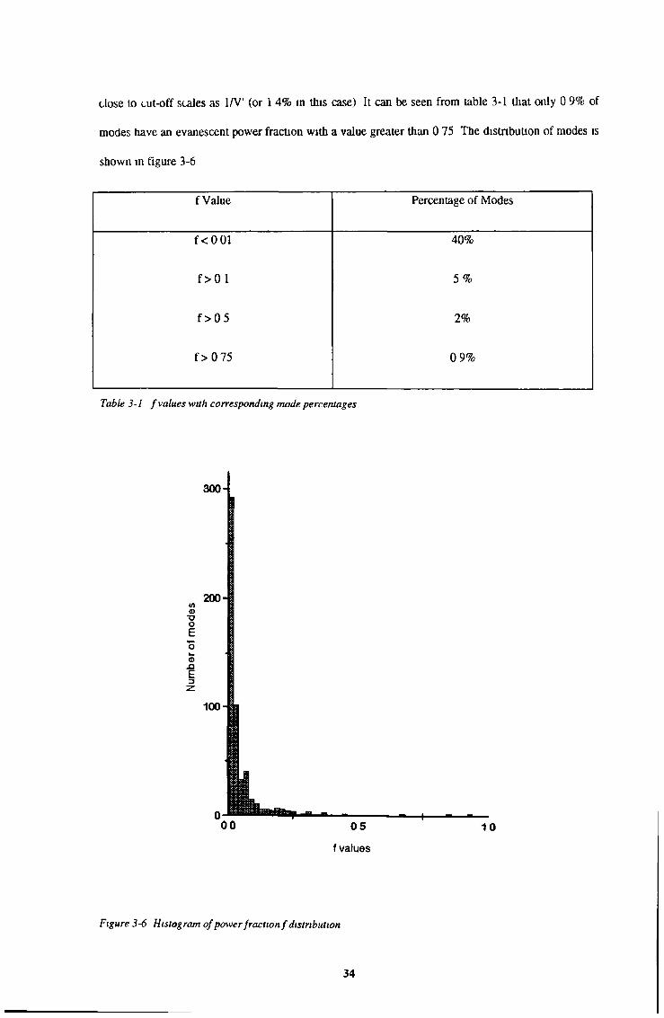
close to cut-off scales as 1/V' (or 1 4% in this case) It can be seen from table 3-1 that only 0 9% of
modes have an evanescent power fraction with a value greater than 0 75 The distribution of modes is
shown in figure 3-6
f Value Percentage of Modes
fcOOl 40%
f > 0 1 5 %
f>0 5 2%
f > 075 0 9%
Table 3-1 f values with corresponding mode percentages
f values
Figure 3-6 Histogram of power fraction f distribution
34
3.7 Dependence of fon V'and (b/a).
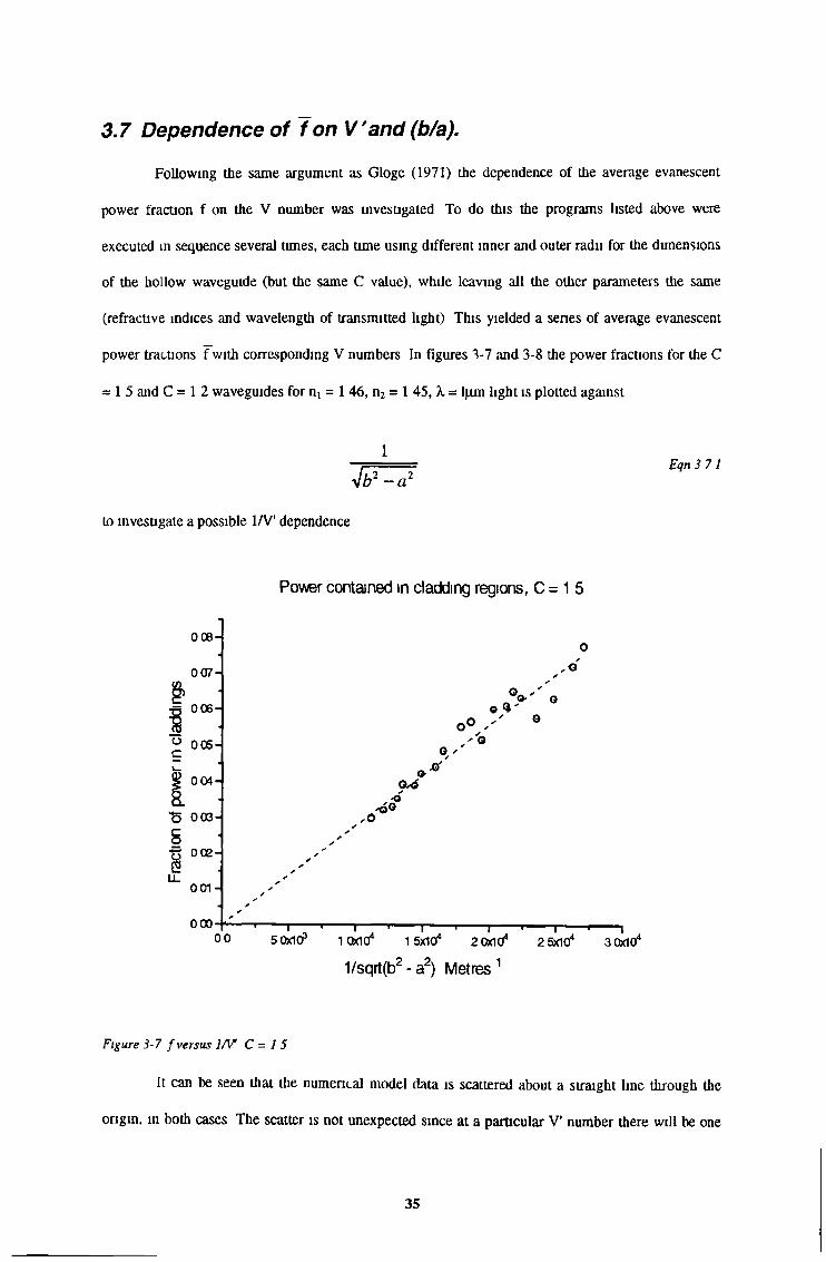
Following the same argument as Gloge (1971) the dependence of the average evanescent
power fraction f on the V number was investigated To do this the programs listed above were
executed in sequence several times, each time using different inner and outer radii for the dimensions
of the hollow waveguide (but the same C value), while leaving all the other parameters the same
(refractive indices and wavelength of transmitted light) This yielded a series of average evanescent
power tractions f with corresponding V numbers In figures 3-7 and 3-8 the power fractions for the C
= 15 and C = 1 2 waveguides for ni = 1 46, n2 = 1 45, X = l tm light is plotted against
1Jb2- a 2
to investigate a possible 1/V' dependence
Power contained in cladding regions, C = 1 5
Eqn 371
Figure 3-7 f versus 1/V C - 1 5
It can be seen that the numerical model data is scattered about a straight line through the
origin, m both cases The scatter is not unexpected since at a particular V' number there will be one
35
mode extremely close to cut-off (W = 0) which will give an unusually high evanescent power fraction
tor that mode
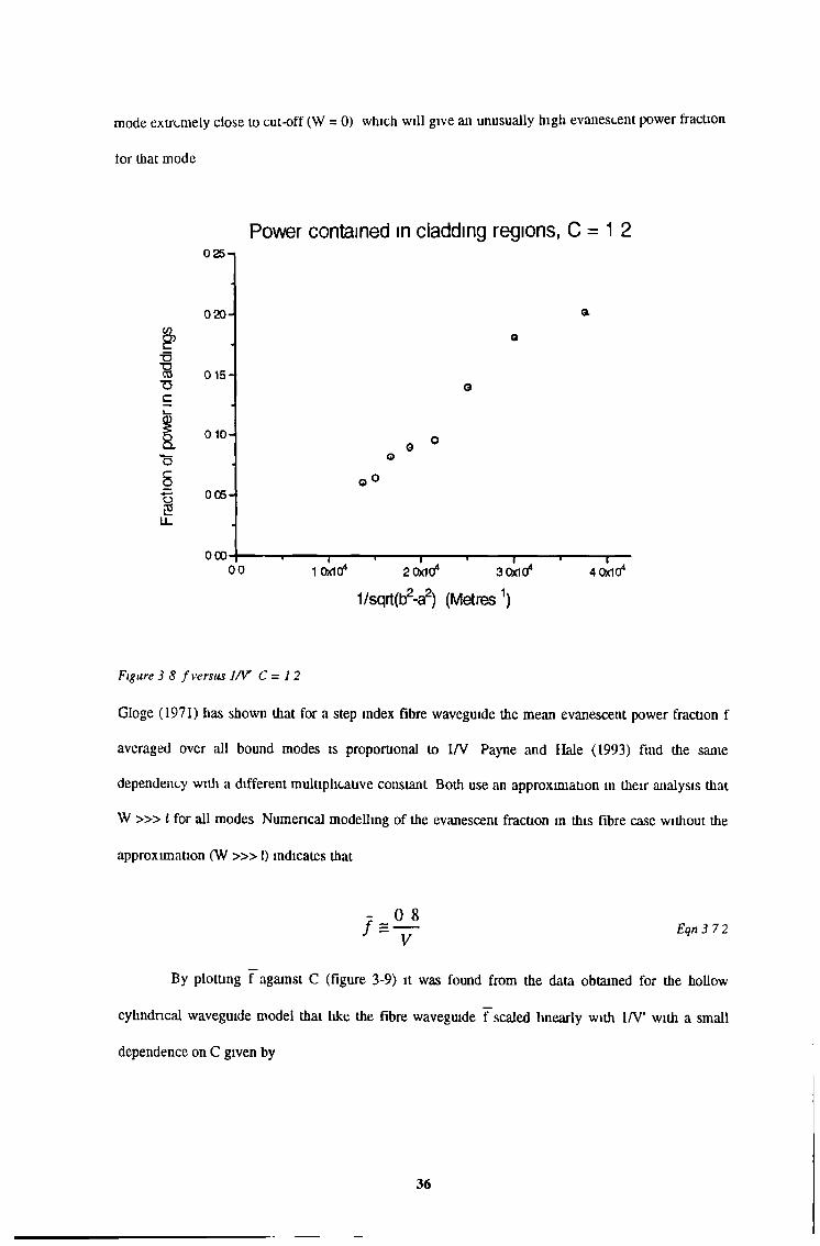
Power contained in cladding regions, C = 1 2
Figure 3 8 f versus 1/V C - 12
Gloge (1971) has shown that for a step index fibre waveguide the mean evanescent power fraction f
averaged over all bound modes is proportional to 1/V Payne and Hale (1993) find the same dependency with a different multiplicative constant Both use an approximation in their analysis that
W » > I for all modes Numerical modelling of the evanescent fraction m this fibre case without the
approximation (W » > t) indicates that
; 0 8/ = — Eqn3 7 2
By plotting f against C (figure 3-9) it was found from the data obtained for the hollow
cylindrical waveguide model that like the fibre waveguide f~scaled linearly with 1/V' with a small
dependence on C given by
36
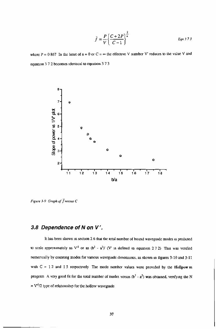
- P [ C + 2P\*
f ~ V { C - l JEqn 3 7 3
where P = 0 867 In the limit of a = 0 or C = «» the effective V number V’ reduces to the value V and
equation 3 7 2 becomes idenucal to equation 3 7 3
Sn
7 A
ts"S. 6- >
$ 5 -
4 -
O 3- CO
2-- T — i----------- 1----1------------ 1--1— |------------- 1--1------------- 1--1--------1 " | i 1---111 12 13 14 15 16 17 18
b/a
Figure 3-9 Graph of f versus C
3.8 Dependence of N on V'.
It has been shown in section 2 6 that the total number of bound waveguide modes is predicted to scale approximately as V'2 or as (b2 - a2)’ (V‘ is defined in equauon 2 7 2) This was verified
numerically by counting modes for various waveguide dimensions, as shown in figures 3-10 and 3-11
with C = 1 2 and 1 5 respectively The mode number values were provided by the Hollpow m
program A very good fit for the total number of modes versus (b2 - a2) was obtained, verifying the N
= V'2/2 type of relationship for the hollow waveguide
37
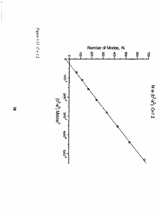
Figure ?-Il
C =
1 2
Number of Modes, N
o § § § § § § §
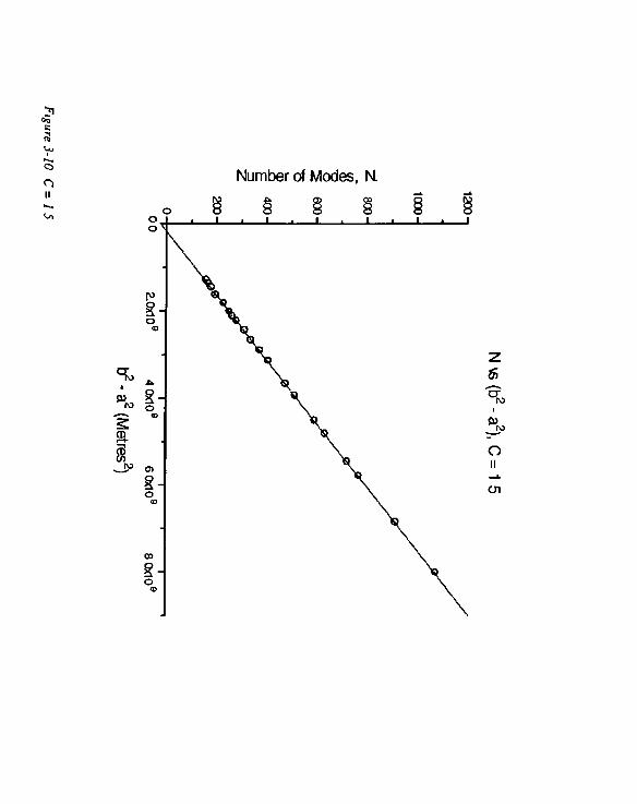
Figure 3-10
C =
1 5
Number of Modes, N.
o § § § § § §
S 1=0
'(se
-zq)
9\N
3.9 Conclusions.
The computer programs listed above represent a model of the effect a hollow cylindrical
waveguide has on light being transmitted through it The model parameters can be varied m terms of
refractive index of the core and cladding, the waveguide dimensions and the wavelength of light being
transmitted through it The model yielded theoretical relationships between the number of modes, N,
the mean evanescent power fraction, f, and the effective V number, V'f and showed the inter
dependence of the various parameters
39
3.10 References.
Gloge D, “Weakly Guiding Fibers”, Appl Opt 10 pp 2252 - 2258 (1971)
Payne F P and Hale Z M, “Deviation from Beer’s Law in Multimode Optical Fiber Evanescent Field
Sensors”, Int J Optoelectronics, 8 (5/6) 743 - 748 (1993)
40
4. Evanescent wave spectrophotometry using a hollow waveguide probe.
4.1 Introduction.The design of an Attenuated Total Reflectance (ATR) Hollow Cylindrical Sensing probe and
an absorbance detection system is described Uniform mode excitation is achieved using a series of
launch step-mdex fibers butt coupled to the ATR probe
4.2 The ATR probe.A length of fused silica hollow tubing of inner diameter (2a) 9 32 m m and outer diameter
(2b) 11 863 m m was chosen as the sensor probe The rod was cut to a length of 280 mm, using a
diamond saw and polished at both ends on a Logitech PM2A Lapping Machine, with a set of water
based grits of decreasing diameter from 10 |im to 1 pm For the polishing the silica was supported in
a stainless steel disk, and kept vertical by strapping to the central shank of the “polishing tree”
Regular inspection of the end (l e cut) surfaces was earned out to ensure that all surface blemishes
were removed by the coarse gnt lapping and polished to a high transparency by the final fine gnt
4.3 Excitation of modes in the probe.As discussed briefly in section 4 1 excitation of the modes in the hollow waveguide was
achieved by butt coupling an array of step index fibers (CeramOptec GmbH OPTRAN H-UV
1000/1035) to one end of the probe This was done using a machined aluminum plug to which the
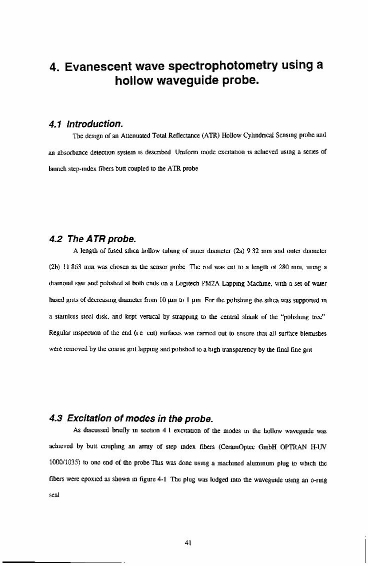
fibers were epoxied as shown in figure 4-1 The plug was lodged into the waveguide using an o-ring seal
41
Fibres
AluminiumPlug
SilicaWaveguide
0-Rings_
42
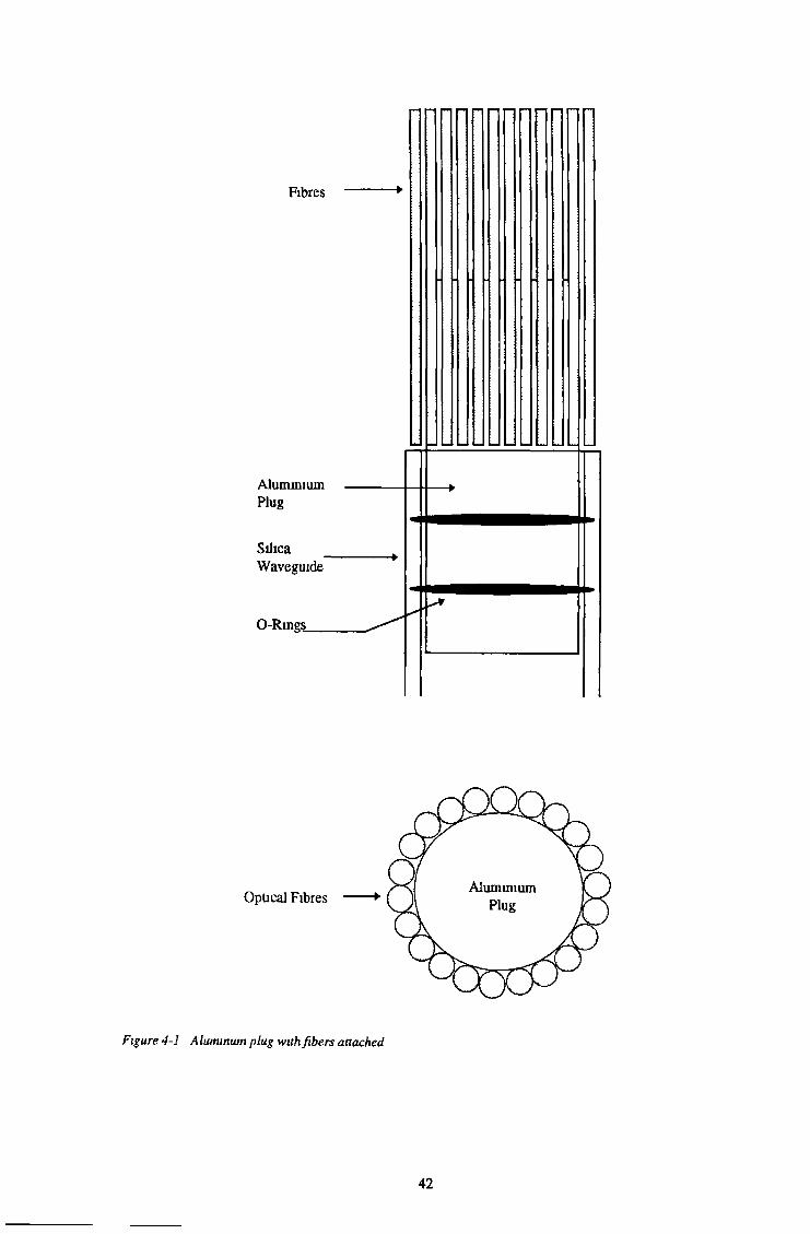
Light from a 20 W Tungsten halogen light source, powered by a 6 V dc supply was focussed
by a 50 mm diameter 65 mm focal length convex-concave lens combinauon (convex effect) into the
fiber bundle as shown m figure 4-2 below To provide stable emittance conditions the lamp was run
below its’ 3 3 A rating, a figure of 2 5 A was found to be sufficient With no liquid surrounding the
probe a bright ring of light was observed at the other end of the probe indicating a uniform excitation
of the modes m the waveguide probe
Concave-convex lens combination
Figure 4-2 Light being focussed into fiber bundle
4.4 Theoretical absorbance of hollow waveguide probe.The probe dimensions listed in 4 1 lead to a value of the dimensionless constant C (= b/a)of
1 2728 from the average values of a series of measurements of a and b The refractive index n! of
fused silica was taken as 1 46 In order to determine the effective V number of the waveguide its’ numerical aperture NA must be determined, l e NA = (nt2 - n22)1/2 The solution used for evaluation
of the probe was Eosm Yellow (C2 0H6 Br4 Na2 05) in Methanol Eosin yellow has an absorption band centred at 524 nm At the concentrations used the refractive index of the solutions were that of
Methanol namely 1 3276 Taking ni = 1 46, n2 = 1 3276 gives a probe numerical aperture of 0 607
Because this numerical aperture is quite large and because the probe was to be excited by light from a
set of step index fibers (of small numerical aperture) butt coupled to one end, the limiting numerical
aperture of the system was the smaller of the two, which m this case was the NA of the fibers This
excitation using fibers will be discussed m a subsequent section Here the value of (n!2 - n22)172 will be
43
taken as the numerical aperture of the fibers, namely 0 37 Using equation 2 7 2 with X = 524 nm the
effective V number of the hollow tube waveguide is then 16281 214 Using equation 3 7 3 the
theoretical mean evanescent power fraction f is then 245 389 x 106 (where P is set at 0 867 and C at
1 2728)
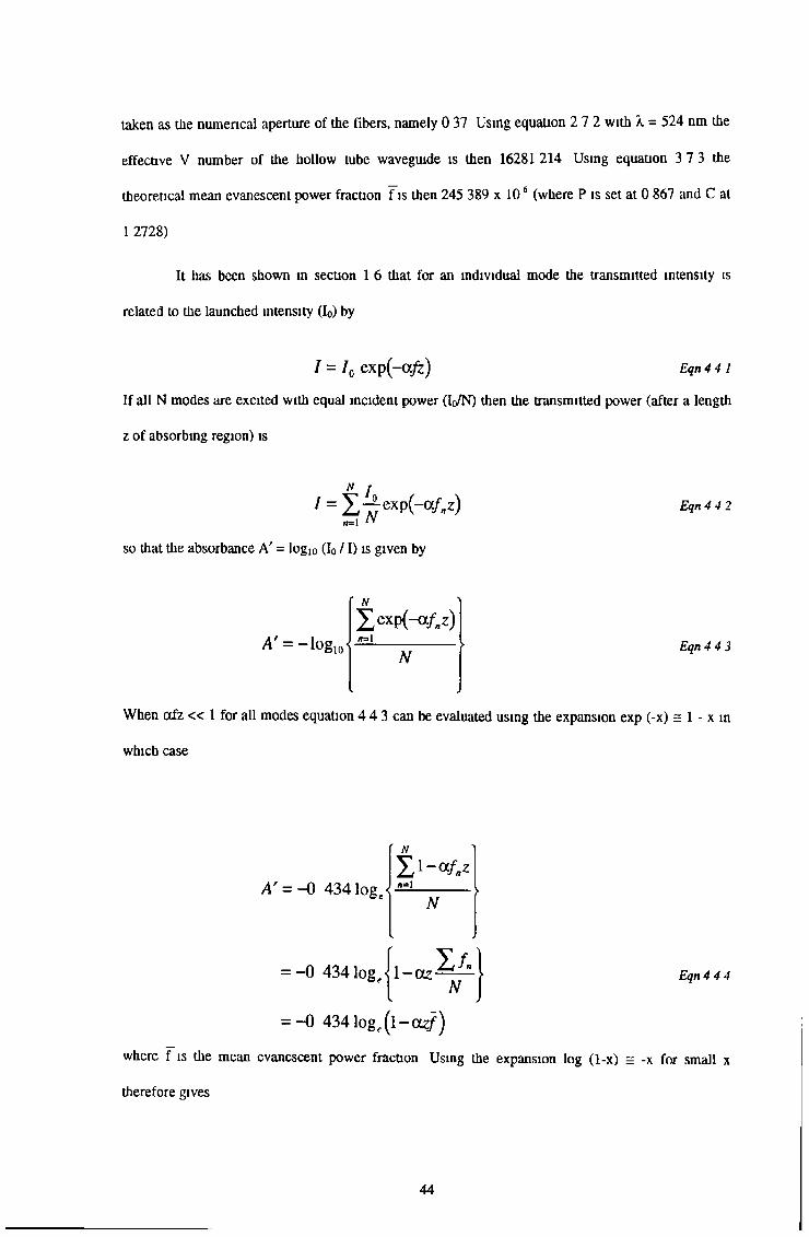
It has been shown in section 1 6 that for an individual mode the transmitted intensity is
related to the launched intensity (I0) by
/ = I0 exp(-OCfc) Eqn 4 41
If all N modes are excited with equal incident power (Io/N) then the transmitted power (after a length z of absorbing region) is
1 = X ^ exp(-oc/„z)*=1 w
so that the absorbance A' = log10 (Io /1) is given by
Eqn 4 4 2
A' = -lo g 10<£ e x p (-qfnz)rp=l
NEqn 44 3
When afz « 1 for all modes equation 4 4 3 can be evaluated using the expansion exp (-x) = 1 - x in which case
A' = - 0 434 log.
= - 0 434 log.
I 1-«/.n=l
N
1 -a zN
Eqn 44 4
= - 0 4341og^(l-oc2f)
where f is the mean evanescent power fraction Using the expansion log (1-x) = -x for small x therefore gives
44
A' = 0 434az/ provided faz« 1 Eqn44 5
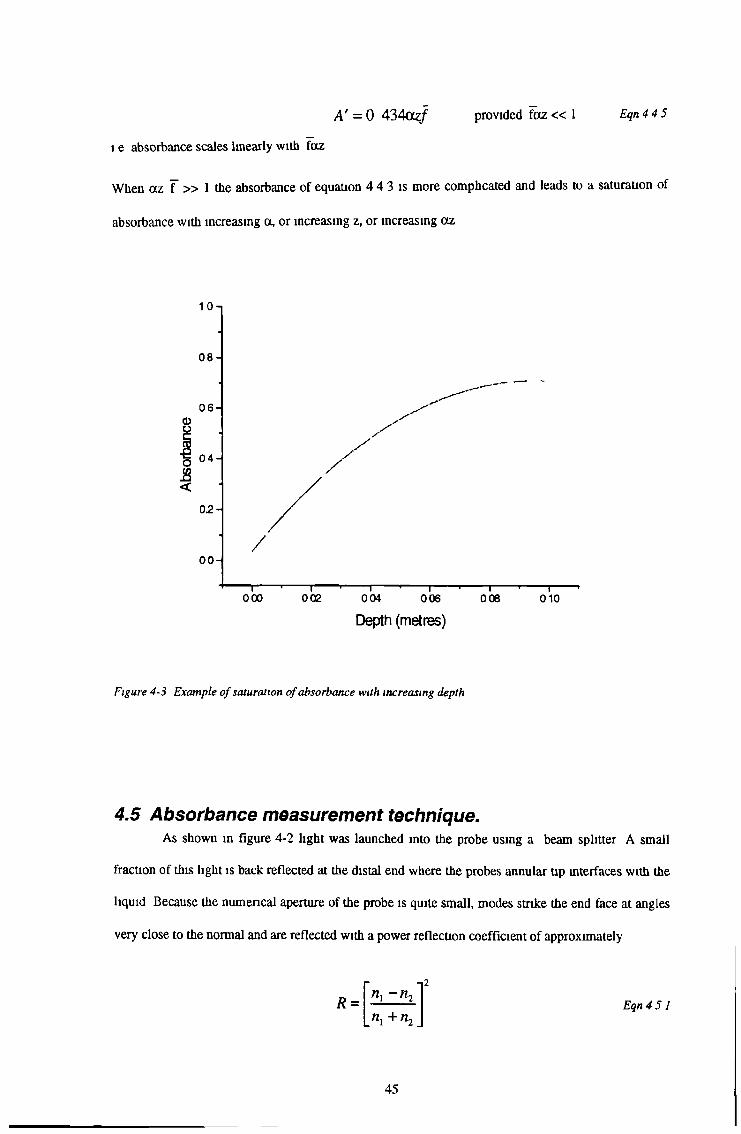
ie absorbance scales linearly with faz
When az T » 1 the absorbance of equation 4 4 3 is more comphcated and leads to a saturation of
absorbance with increasing a, or increasing z, or increasing az
Depth (metres)
Figure 4-3 Example of saturation of absorbance with increasing depth
4.5 Absorbance measurement technique.As shown in figure 4-2 light was launched into the probe using a beam splitter A small
fraction of this light is back reflected at the distal end where the probes annular tip interfaces with the
liquid Because the numerical aperture of the probe is quite small, modes strike the end face at angles
very close to the normal and are reflected with a power reflection coefficient of approximately
R = nx -n2
n\ +n2Eqn 4 51
45
(the Fresnel reflection coefficient for normal incidence) [It is shown in Appendix G that for a
practical range of incident angles 0i the reflection coefficient R is approximately independent of 0,]
If an intensity I0 is launched into the probe (at a wavelength X) then Io exp (- faz) reaches
the endface, Ro Io exp (- faz) is reflected and Ro I0 exp (-2 faz) is returned to the launch fibers This
is based on absorption occunng at an analytical wavelength At a wavelength well removed from the
absorption band - the so-called reference wavelength - a back reflected intensity of R Io occurs (1 e no
atttenuation) Thus an evanescent power absorbance (A') of
is obtained This is the previously derived expression of equation 4 4 5 but doubled for 2 way travel of
the evanescent wave along the probe length z As before equation 4 5 2 apphes provided faz « 1 As
previously defined a is the bulk attenuation coefficient of the absorber and z is the immersion depth of
the probe in the absorber By comparing the back-reflected light intensity at the analytical and
reference wavelength then the absorbance of the probe can be measured
Two interference filters were used to isolate a wavelength band centered at X = 525 nm
(where Eosm Yellow has an absorption band) and X = 430 nm in the blue to one side of the absorption
band The filters were supported on a mechanical slide and could be placed in turn in front of the
entrance window of a Hamamatsu 931A photomultiplier tube The photomultiplier was operated in
the “grounded anode” mode, the detector signal being extracted as a voltage across a 10M ft resistor
The light entering the launch fibers was modulated using a mechanical chopper which operated at a
chopping frequency of 330 Hz The chopper drive unit (Scitec Instruments optical chopper) supplied
the square wave pulse train to synchronise phase sensitive detection with a lock-in amplifier The PM
output was fed by coaxial cable to the signal input of an EG&G model lock-in amplifier (model
950VG) whose post filter time constant was set at 3 seconds
An absorbance measurement then involved recording two output voltages from the lock-in
amplifier corresponding to each optical filter being in the light beam returning to the photomultiplier
Rl,E q n 4 5 2
= (0 434)(2jixz), faz « 1
46
detector A series of back reflected intensity measurements, with the probe enclosed in a light tight
box, was made to determine if any drift occured m either (1) the light source intensity or (11) the
photomultiplier output It was found that the lamp intensity stabilised in 45 minutes after switching
on, and there was no detectable photomultiplier drift over a 2 hour period The PM was powered by a
500 V EHT unit (EMI electron tube division Power Supply PM28B)
4.6 Conclusions.A relatively simple back-reflection ATR probe, excited by light from a tungsten halogen
lamp via an array of step index fibers butt coupled to one end and operated in phase sensitive
detection, was constructed The evanescent light in both the inner hole and surrounding medium may
be used to analyse fluids with absorption bands m the visible using a dip-suck style of approach All
optics are concentrated at one end of the probe
47
5. Experimental absorbances using hollowsilica waveguide.
5.1 Introduction.Absorbance measurements made with the ATR analyser probe discussed in chapter 4 are
reported here Results are compared to the mode model predictions of chapters 2 and 3
5.2 Bulk properties of the absorbing cladding.As stated earlier a solution of Eosin Yellow in Methanol was chosen as the absorbing
cladding with which the hollow cylindrical ATR probe was to be evaluated The bulk absorption
properties of this chemical at X = 524 nm were examined using a SHIMADZU (UV - 1201) UV-VIS
spectrophotometer Solutions of various molar concentrations (1M = 0 69186 gram/cc of solute) were
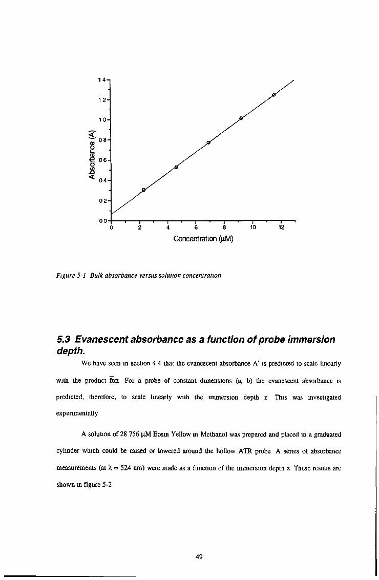
prepared and their bulk absorbances (at 524 nm) were measured In each case a cuvette containing the solution was inserted in the spectrophotometer beam and the beam attenuation compared to that of the
solute (methanol) on its own A graph of absorbance versus solution concentration (figure 5-1) was
prepared and a least-square fit line generated throught the data points (using an “Origin” subroutine)
From the best-fit slope the bulk absorption coefficient a for Eosin Yellow was found For a 1M
solution a was found to be a = 23250 0 m m 1 (or 0 02325 m m 1 jiM l)
For a weaker solution - say of concentration 103 M, the corresponding a value is 1000 times
smaller For evanescent wave absorption the parameter of interest is 7a, where F is the mean evanescent power fraction among the modes
48
Concentration (nM)
Figure 5-1 Bulk absorbance versus solution concentration
5.3 Evanescent absorbance as a function of probe immersion depth.
We have seen in section 4 4 that the evanescent absorbance A' is predicted to scale linearly
with the product fotz For a probe of constant dimensions (a, b) the evanescent absorbance is
predicted, therefore, to scale linearly with the immersion depth z This was investigated experimentally
A solution of 28 756 p.M Eosin Yellow in Methanol was prepared and placed in a graduated
cylinder which could be raised or lowered around the hollow ATR probe A series of absorbance
measurements (at X = 524 nm) were made as a function of the immersion depth z These results are
shown in figure 5-2
49
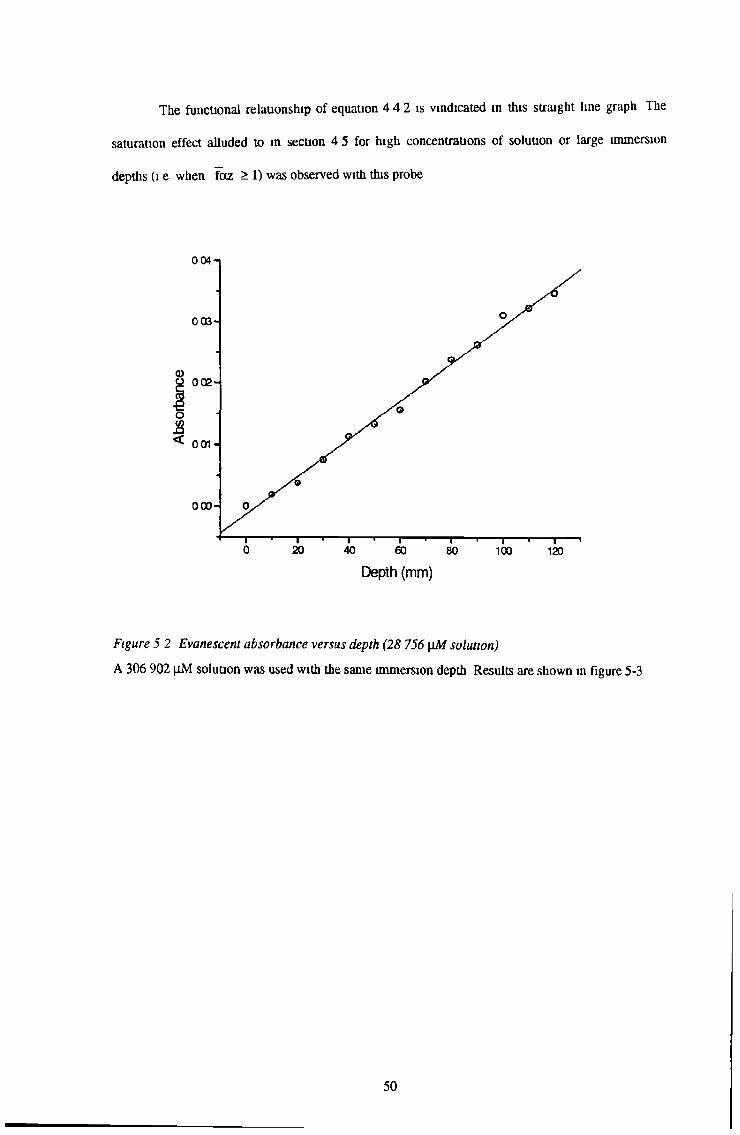
The functional relationship of equation 4 4 2 is vindicated in this straight line graph The
saturation effect alluded to in section 4 5 for high concentrations of solution or large immersion
depths (i e when faz > 1) was observed with this probe
Depth (mm)
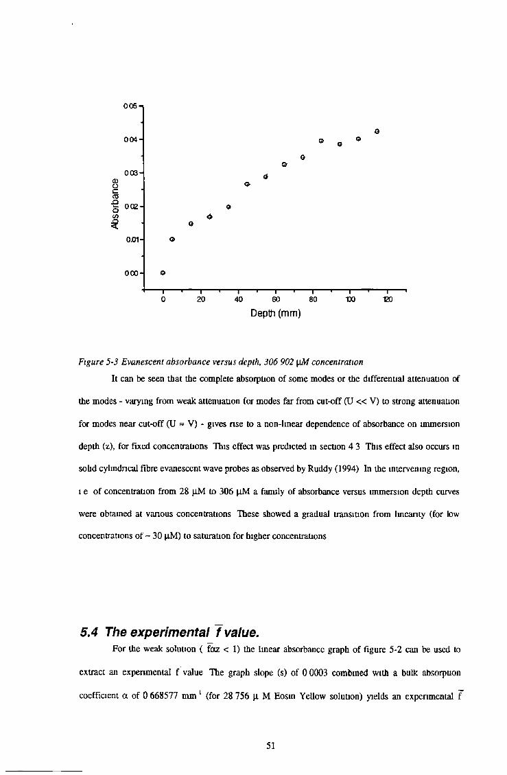
Figure 5 2 Evanescent absorbance versus depth (28 756 \xM solution)A 306 902 tM solution was used with the same immersion depth Results are shown in figure 5-3
50
I
Depth (mm)
Figure 5-3 Evanescent absorbance versus depth, 306 902 \xM concentrationIt can be seen that the complete absorption of some modes or the differential attenuation of
the modes - varying from weak attenuation for modes far from cut-off (U « V) to strong attenuation
for modes near cut-off (U » V) - gives rise to a non-lmear dependence of absorbance on immersion
depth (z), for fixed concentrations This effect was predicted in section 4 3 This effect also occurs in
solid cylindrical fibre evanescent wave probes as observed by Ruddy (1994) In the intervening region,
i e of concentration from 28 |iM to 306 |iM a family of absorbance versus immersion depth curves
were obtained at various concentrations These showed a gradual transition from linearity (for lowconcentrations of ~ 30 |xM) to saturation for higher concentrations
5.4 The experimental f value.For the weak solution ( fotz < 1) the linear absorbance graph of figure 5-2 can be used to
extract an experimental f value The graph slope (s) of 0 0003 combined with a bulk absorption
coefficient a of 0 668577 m m 1 (for 28 756 \i M Eosm Yellow solution) yields an experimental f
51
value of 224 3571 xlO"6 This may be compared to the theoretical value of equation 3 7 3 taking P =
0 867, C = 1 2728, V' = 16281 214 of f = 245 38957 xlO*6 This is a difference of 8 57% It can be
seen that the mode modelling ot chapters 2 and 3 and the experimental measurement of chapter 5 are
m very good agreement
5.5 Conclusions.Experimental measurements of absorbance using a hollow cylindrical ATR probe were used
to extract a mean evanescent power fraction ( 0 among all the bound modes of the waveguide Good
correlation between the experimentally derived f values and that predicted by rigorous mode analysis
for such a waveguide indicates the latter It should be stated that the mode analysis earned out does
not assume the “weakly guiding” approximation (n! = n2) as in general with glass based probes and
liquid absorber solutions that approximation (commonly used in step-index fibre mode analysis) is not valid
52
5.6 References.Ruddy V, "Non linearity of absorbance with sample concentration and path length m evanescent
wave spectroscopy using optical fibre sensors”, Optical Engineenng 33, no 12, pp (3891-2893)
(1994)
53
Appendix A
The following is the Matlab code for the Cuts m program Any lines starting with a ‘% ’ sign are comments on the code, not part of the code itself, and are ignored by the Matlab compiler
% Title Cutsm
% Aim To calculate cut off values for a hollow cylindrical % waveguide by stepping through the cut
% off equation until the zeros are located
de!ta_x =1, % step size in U
xl = 1, % starting value for U
for j =0 j_max, % loop through all orders, where j is the order t
count = 1, % resets the count of U values in each I order
yl = cutout(j,xl,C), % calculate value of cut-off equation
while (xl < x_max), % step through all U values
x2 = xl + delta_x, % increment U by delta U
limit = x2, % stores largest U value tested so far
y2 = cutout(j,x2,C), % calculate value of cut-off equation
test = xl, % stores next largest U value tested so far
if ((y2/yl) < 0), % if sign change occurs, root is isolated
while (test < limit),
x2 = xl + (delta_x/10), % increase U value by 10% of delta U
y2 = cutout(j x2 C) % calculate value of cut-off equation
if (y2/yl) > 0, % if sign change has not occured
end,
if count
end,
if J >0,
xl = x2 + delta_x/10, % increase U value by 10% of
% delta U
yl = cutout(j,xl,C), % calculate value of cut-off% equation
else
slope = (y2 - yl)/(x2 - xl), % sign change has occured
U = xl - (y 1/slope), % calculate correct root value
ucut(j+l,count) = U, % save U value in array
count = count + 1, % increment counter
test = limit+1, % make ‘test’ > ‘limit’
end, % end of 4if(y2/yl) > 0’ statement
yl = y2, % prepare for next run through loop
xl = x2, % prepare for next run through loop
end,
else
yl = y2, % prepare for next nm through loop
xl = x2, % prepare for next run through loop
end, % end of ‘while (test < limit),’ statement
% end of ‘if (y2/yl) < 0)’ statement
== 1, % if no cutoffs are found
break, % exit ‘while (xl < x_max),’ loop
A-2
if ucut(j,l) < x_max, % if all roots of present order I have not yet been tound,
xl = ucut(j+l,l), % start searching at last known U value
end,
else
xl = 6, % reset to lowest U value, to search next I order
end,
ucut(j,) % output to screen all found U values
end, % end of ‘j =0 j_max’ loop
A-3

Appendix B
This program evaluates the cut-off equation at values passed to it from the program that called it in
this case the calling program is Cuts m
% Title Cutout m
% Aim To calculate value of cut off equation at a given U value
function[y_val] = cutout(j,x?C) % defines the function name and the number and value of variables % the function will use
yl = (besselj(j,x) * bessely(j,C*x)), % defines the equation parts used in the function
y2 = (besselj(j,C*x) * bessely(j,x)),
y_val = yl - y2, % calculates the value of the function at the specified parameter values,
% and returns this value to the calling program
B-l
Appendix C
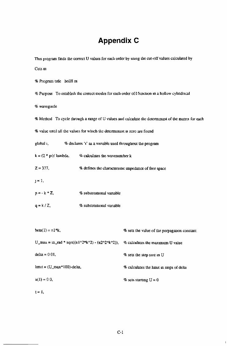
This program finds the correct U values for each order by using the cut-off values calculated by
Cuts m
% Program title holl8 m
% Purpose To establish the correct modes for each order of t function m a hollow cylindrical
% waveguide
% Method To cycle through a range of U values and calculate the determinant of the matrix for each
% value until all the values for which the determinant is zero are found
global 1, % declares V as a variable used throughout the program
k = (2 * pi)/ lambda, % calculates the wavenumber k
Z = 377, % defines the characteristic impedance of free space
p = -k*Z, % substitutional variable
q = k / Z, % substitutional variable
beta(l) = nl*k, % sets the value of the porpagation constant
U_max = in_rad * sqrt((n 1 A2*kA2) - (n2A2*kA2)), % calculates the maximum U value
delta = 0 01, % sets the step size in U
limit = (U_max*100)-delta, % calculates the limit in steps of delta
u(l) = 0 0, % sets starting U = 0
t = 1,
C-l
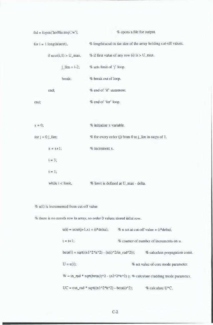
fid = fopenChollSa.tmpVw'); opens a file for output.
for i = l:length(ucut), length(ucut) is the size of the array holding cut-off values.
if ucut(i,l) > U_max, % if first value of any row (i) is > U_max.
j_lim = i-2;
break;
end;
end;
sets limit of ‘j’ loop,
break out of loop,
end of ‘if statement,
end of ‘for’ loop.
x = 0; % initialise x variable.
for j = 0:j_lim; % for every order (j) from 0 to j_lim in steps of 1.
x = x+1; % increment x.
i = 3;
t= 1;
while i < limit, % limit is defined at U_max - delta.
% u(i) is incremented from cut off value
% there is no zeroth row in array, so order 0 values stored in 1st row.
u(i) = ucut(j+l,x) + (t*delta); % u set at cut-off value + (t*delta),
t = t+1; % counter of number of increments on u.
beta(i) = sqrt((nlA2*kA2) - (u(i)A2/in_radA2)); % calculate porpagation const.
U = u(i); % set value of core mode parameter.
W = in_rad * sqrt(beta(i)A2 - (n2A2*kA2)); % calculate cladding mode parameter.
UC = out_rad * sqrt((nlA2*kA2) - beta(i)A2); % calculate U*C.
C-2
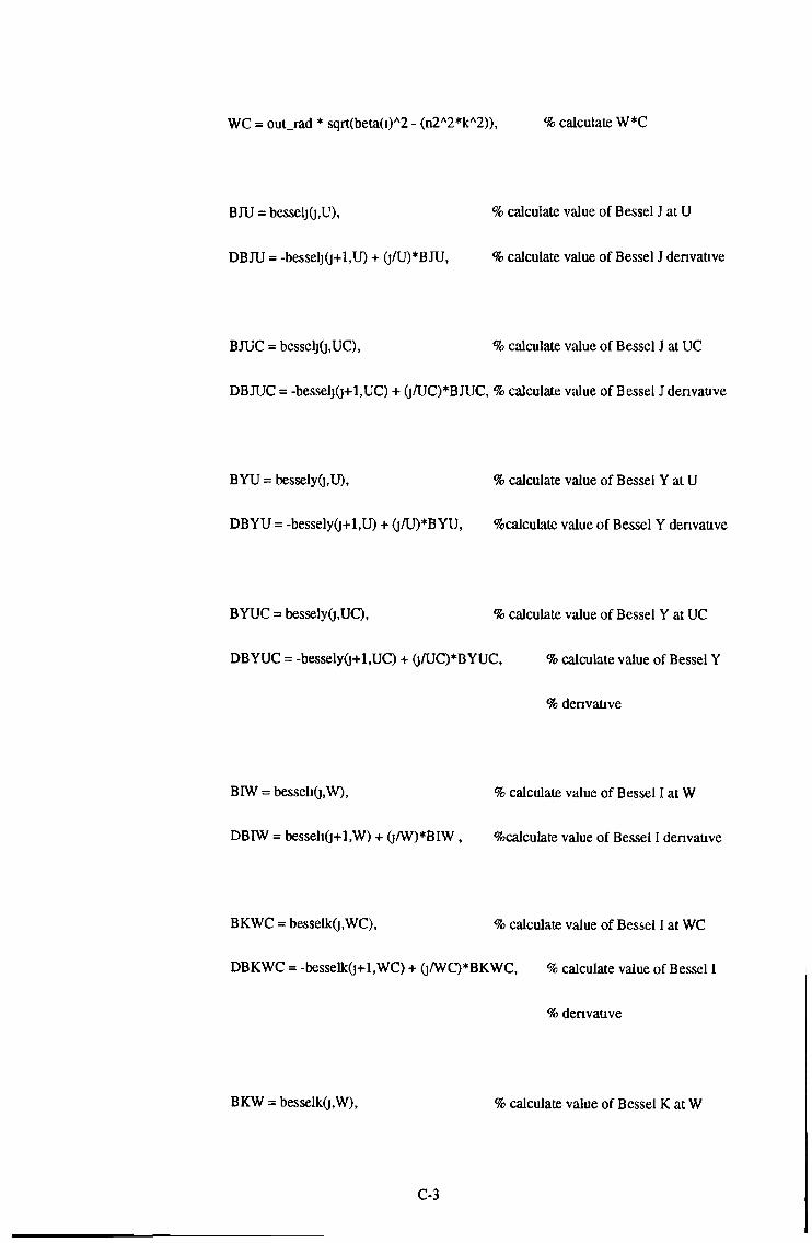
W C = out_rad * sqrt(beta(i)A2 - (n2A2*kA2)), % calculate W*C
BJU = besselj(j,U), % calculate value of Bessel J at U
DBJU = -besselj(j+l,U) + °t° calculate value of Bessel J derivative
BJUC = besseljO,UC), % calculate value of Bessel J at UC
DBJUC = -besselj(j+l,UC) + (j/UC)*BJUC, % calculate value of Bessel J derivative
BYU = bessely(j,U), % calculate value of Bessel Y at U
DBYU = -bessely(j+l,U) + YU, calculate value of Bessel Y derivative
BYUC = bessely(j,UC), % calculate value of Bessel Y at UC
DBYUC = -bessely(j+l,UC) + (j/UC)*BYUC, % calculate value of Bessel Y
% derivative
BIW = besseli(j,W), % calculate value of Bessel I at W
DBIW = besseli(j+l,W) + (j/W)*BIW , calculate value of Bessel I denvauve
BKWC = besselk(j,WC), % calculate value of Bessel I at WC
DBKWC = -besselk(j+l,WC) + (j/WC)*BKWC, % calculate value of Bessel I
% denvauve
BKW = besselk(j,W), % calculate value of Bessel K at W
C-3
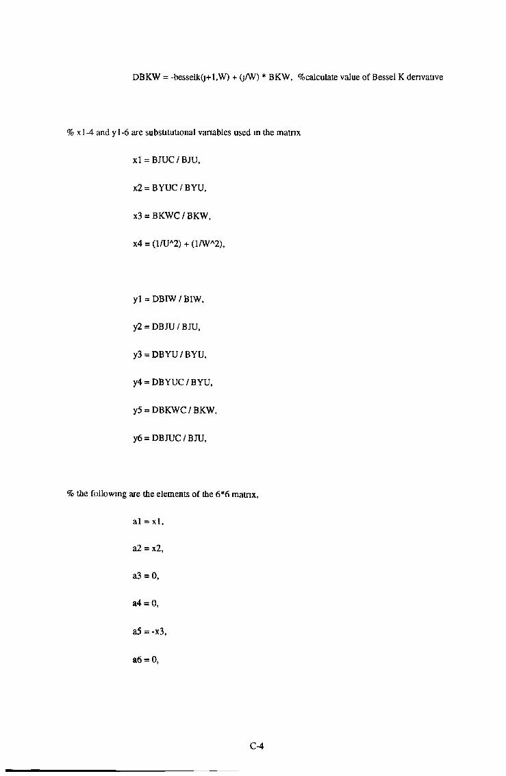
D B K W = -besselk(j+l,W) + (j/W) * BKW, %calculate value of Bessel K derivative
% xl-4 and yl-6 are substitutional variables used in the matrix
xl = BJUC / BJU,
x2 = BYUC / BYU,
x3 = BKWC / BKW,
x4 = (1/UA2) + (1/WA2),
yl = DBIW / BIW,
y2 = DB JU / BJU,
y3 = DBYU/BYU»
y4 = DBYUC / BYU,
y5 = DBKWC / BKW,
y6 = DB JUC / BJU,
% the following are the elements of the 6*6 matrix,
al = xl,
a2 = x2,
a3 = 0,
a4 = 0,
a5 = -x3,
a6 = 0,
C-4
bl = O,
b2 = O,
b3 = xl,
b4 = x2,
b5 = 0,
b6 = -x3,
cl = (-beta(i) * j) * x4,
c2 = (-beta(i) * j) * x4,
c3 = ((p/W)*yl) + ((p/U)*y2),
c4 = ((p/W) * yl) + ((p/U) * y3),
c5 = 0,
c6 = 0,
dl = ((q * n2A2 * yl) / W) + ((q * nlA2 * y2) / U),
d2 = ((q * n2A2 * yl) / W) + ((q * nlA2 * y3) / U),
d3 = beta(i) * j * x4,
d4 = beta(i) * j * x4,
65 = 0,
d6 = 0,
el = (beta(i) * j * xl) / (UA2 * C),
e2 = (beta(i) * j * x2) / (UA2 * C),
C-5
e3 = (-p*y6)/U,
e4 = (-p * y4) / U,
e5 = (beta(i) * j * x3) / (WA2 * C),
e6 = (-p*y5)/W,
fl = (-q * nlA2 * y6) / U,
f2 = (-q * nlA2 * y4) / U,
f3 = (-beta(i) * j * xl)/ (UA2 * C),
f4 = (-beta(i) * j * x2) / (UA2 * C),
f5 = (-q*n2A2*y5)/W,
f6 = (-beta(i) * j * x3) / (WA2 * C),
matrl = [ al a2 a3 a4 a5 a6
blb2b3b4b5 b6
cl c2 c3 c4 c5 c6
dl d2 d3 d4 d5 d6
el e2 e3 e4 e5 e6
n f2 f3 f4 f5 f6], % places each element in the matrix
deter(i) = det(matrl),
m(i) = deter(i)/deter(i-l),
% calculates the determinant of the matrix
% divides determinany value of matrix by
if (m(i) < 0 0),
previous determinant value
if sign change has occured
C-6
if (deter(i-2)) ~= 0 0, % eliminates false roots
U_t(j+l,x) = u(i) - ((deter(i) * delta) / (deter(i) - deter(i-l))),
% calculates exact value of core mode parameter
beta_t(x) = sqrt((nlA2*kA2) - (U_t(j+l,x)A2/in_radA2)),
% calculates value of corresponding propagation constant
W_t(j+l,x) = in_rad* sqrt(beta_t(x)A2 - (n2A2*kA2)),
% calculates value of corresponding cladding mode parameter
fpnntf(fid,'% Of %0f %f %fW,j,x,lLt(j+l,x),W_t(j+l,x)),
% prints f, m, U and W to the output file
flag = 1, % l needs to be incremented by 10
save djc mat, % saves all variables m the workspace
end, % end of true roots ‘if statement
end, % end of sign change ‘if statement
if flag ==1, % if a root has been found
x = x + 1, % increment mode count
t = 1, % reset delta step size to 1
i = i+10 % to separate stored determinant values in ‘deter’ array
flag = 0, % reset flag
end, % end of positive flag ‘if statement
i = i+l, % increment Y counter
ux = ucut(j+l,x) + (t*delta) + 0 01,% ux is a variable used for checking
if ux >= (U_max - 2*delta) % if the next cut-off value is greater than
C-7

end,
end,
fclose('air),
l = limit, % to break out of loop
x = 0, % reset mode counter
u = u*0, % reset u array
deter = deter*0, % reset deter array values
end, % end of if loop
% end of ‘while 1 < limit’ loop
% end of ‘for j =s 0 j_lim’ loop
% closes all open files
C-8
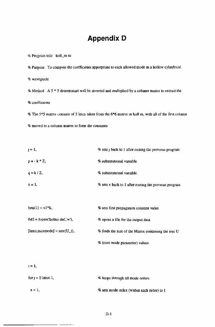
Appendix D
% Program title holl_se m
% Purpose To compute the coefficients apporpnate to each allowed mode m a hollow cylindrical
% waveguide
% Method A 5 * 5 determinant will be inverted and multiplied by a column matrix to extract the
% coefficients
% The 5*5 matrix consists of 5 Imes taken from the 6*6 matrix in holl m, with all of the first column
% moved to a column matrix to form the constants
j = 1, % sets j back to 1 after exiting the previous program
p = - k * Z, % substitutional variable
q = k / Z, % substitutional variable
x = 1, % sets x back to 1 after exiting the previous program
beta( 1) = nl *k, % sets first propagation constant value
fid2 = fopen('hollse dat’/w'), % opens a file for the output data
[IimiUnaxmode] = size(U_t), % finds the size of the Matrix containing the true U
% (core mode parameter) values
i=l,
for j = 0 limit-1, % loops through all mode orders
x — 1, % sets mode index (within each order) to 1
D-l
while x <= maxmode,
eoe = eoe * 0; % matrix to hold coefficient values set to zero.
U = U_t(j+l,x); % U value is retrieved from thè holding matrix.
beta(i) = sqrt((nlA2*kA2) - (UA2/in_radA2)); % claculates thè propagation constant.
W = W_t(j+l,x); % W value is retrieved from thè holding matrix.
UC = out_rad * sqrt((nlA2*kA2) - beta(i)A2); % calculâtes U*C.
W C = out_rad * sqrt(beta(i)A2 - (n2A2*kA2)); % calculâtes W*C.
BJU = besselj(j,U); % calculâtes value of bessel J at U.
DB JU = -besselj(j+l,U) + (j/U)*BJU; % calculâtes derivative of bessel J at U.
B JUC = besselj(j,UC); % calculâtes value of bessel J at UC.
DBJUC = -besselj(j+l,UC) + (j/UC)*BJUC; % calculâtes derivative of bessel J at UC.
B YU = bessely(j,U); % calculâtes value of bessel Y at U.
DBYU = -bessely(j+l,U) + (j/U)*B YU; % calculâtes derivative of bessel Y at U.
B YUC = bessely(j,UC); % calculâtes value of bessel Y at UC.
DBYUC = -bessely(j+l,UC) + (j/UC)*BYUC; % calculâtes derivative of bessel Y at UC.
BIW = besseli(j,W); % calculâtes value of bessel I at W.
DBIW = besseli(j+l,W) + (jAV)*BIW ; % calculâtes derivative of bessel I at W.
D-2
BKWC = besselk(j,WC), % calculates value of bessel K at W C
DBKWC = -besse!k(j+l,WC) + (j/WC)*BKWC, % calculates derivative of bessel K at WC
BKW = besselk(j,W), % calculates value of bessel K at W
DBKW = -besselk(j+l,W) + (j/W) * BKW, % calculates derivative of bessel K at W
% xl-4 and y 1-6 are substitutional variables used m the matrix
xl = BJUC / BJU,
x2 = BYUC / BYU,
x3 = BKWC/BKW,
x4 = (1/UA2) + (1/Wa2)t
yl = DBIW / BIW,
y2 = DBJU/BJU,
y3 = DBYU / BYU,
y4 = DB YUC / BYU,
y5 = DBKWC/BKW,
y6 = DB JUC / BJU,
if j == 0, % for zero order modes only separatemethod is
tempi = ((n2A2 * yl)/W) + ((nlA2 * y2)/U), % used to calculate coefficients
D-3
temp2 = ((n2A2 * yl)/W) + ((nlA2 * y3)/U),
coe(l) = (-tempi)/(temp2), % first coefficient is found
coe(4) = (xl + (x2 * coe(l))) / x3, % fourth coefficient is found
coe(2) = 0, % all others are set to zero
coe(3) = 0,
coe(5) = 0,
else % if mode order is not zero
% the following are the elements of the 5*5 matrix,
a2 = x2,
a3 = 0,
a4 = 0,
a5 = -x3,
a6 = 0,
c2 = (-beta(i) * j) * x4,
c3 = ((p/W) * yl) + ((p/U) * y2)t
c4 = ((p/W) * yl) + ((p/U) * y3),
c5 = 0,
c6 = 0,
d2 = ((q * n2A2 * yl) / W) + ((q * niA2 * y3) / U),
d3 = beta(i) * j * x4,
d4 = beta(i) * j * x4,
D-4
d5 = 0,
d6 = 0,
e2 = (beta(i) * j * x2) / (UA2 * C),
e3 = (-p * y6) / U,
e4 = (-p*y4)/U,
e5 = (beta(i) * j * x3) / (WA2 * C),
e6 = (-p*y5)/W,
f2 = (-q * nlA2 * y4) / U,
f3 = (-beta(i) * j * xl) / (UA2 * C),
f4 = (-beta(i) * j * x2) / (UA2 * C),
f5 = (-q * n2A2 * y5) / W,
f6 = (-beta(i) * j * x3) / (WA2 * C),
matrl = [ a2 a3 a4 a5 a6 % puts each element of the 5*5 matrix in the correct
c2 c3 c4 c5 c6 % position
d2 d3d4d5 d6
e2 e3 e4 e5 e6
f2 f3 f4 f5 f6 ],
% the folowing are the elements of the column matnx
al = -xl,
cl = (beta(i) * j) * x4,
D-5
dl = ((-q * n2A2 * yl) / W) - ((q * nlA2 * y2) / U),
el = (-beta(i) * j * xl) / (UA2 * C),
fl = (q * nlA2 * y6) / U,
matr2 = [al, cl, dl, el, fl], % sets up the column matrix
coe = matrl \ matr2, % multiplies inverse of matrl by column matrix
end, % the ‘V is a special matlab character for this operation
fpnntf(fid2/\n% Of % Of %4f % 4f,j,x,U_tO+l,x),W_t(j+l,x)),
fpnntf(fid2,' % 5f % 5f % 5f % 5f % 5f\n,,coe(l),coe(2),coe(3),coe(4),coe(5)),
% the order, mode index m, U value, W value and the corresponding coefficients are output to a file
if x < maxmode, % if the last mode in a given order has not been reached
if U_t(j+l,x+l) == 0, % if the next mode of that order is zero
x = maxmode+1, % make x > maxmode
end,
end, % end of ‘x < maxmode’ loop
x = x+1, % increment x
end, % end of ‘while x <= maxmode’ loop
end, % end of ‘for j = 0 limit-1’ loop
fclose('air), % close all open files
save c \hollse mat % save variable values in a matlab workspace file
D-6
Appendix E
% Title hollpow m
% Object To calculate the power ratio in a hollow cylindrical waveguide
% Method To numerically integrate over all allowed modes in annulus
j = 1, % set mode order no back to 1
p = - k * Z, % substitutional variable
q = k / Z, % substitutional variable
x = 1, % set mode order index to 1
beta(l) = nl*k, % set first value of propagation constant
AA= 1,
the
% AA is first coefficient, and was set to 1 in previous program to enable
% calculation of the other coefficients
fid = fopen(’hollse dat'/r'), opens the file to which Hollse m saved the results of its run
in_data = fscanf(fid,'%f\n'), % reads in the data as one column
fclose(fid), % closes the file
limit = length(in_data), % calculates the number of variables in the column of data
i = l, % set index equal to 1, the first element of the data column
while i <= limit, % read in nine values for each single mode
j = m_data(i), % each mput value is assigned a label and stored
E-l
x = in_data(i+l),
U_t(j+l>x) = in_data(i+2),
Wj(j+l,x) = in_data(i+3),
BB(j+l,x) = in_data(i+4),
CCQ+l,x) = in_data(i+5),
DD(j+l,x) = in_data(i+6),
EE(j+l,x) = in_data(i+7),
FF(j+l,x) = in_data(i+8),
1 = 1+9, % index incremented by nine to the next set of nine values
end, % end of data storage loop
j Jimit = m_data(i-9), % sets the maximum value of j
[qwe,x_limit] = size(U_t), % finds the size of the array holding the U values
U_t(j Jimit,x_limit+l) = 0, % increases the array columns by 1, and sets that column = 0
fidl = fopen('holJpow5 datVw’X % opens a file for output data
FI =0,
F2 = 0,
F3 = 0,
mode_count = 0,
forj = OjJimit,
x = 0,
the variables that will store the power fractions are set to 0
while x < x Jimit,
x = x + 1,
the mode counter is set to 0
loop through all the mode orders
% sets mode index to 0
while mode index is less than its maximum value
increment mode index
E-2
U s= U_t(j+l,x), % retneve corresponding U value
W = W_t(j+l,x), % retneve corresponding W value
beta = sqrt((nlA2*kA2) - (UA2/in_radA2)), % calculate corresponding prop const
BJU = besselj(j,U), % calculates bessel J at U
DB JU = -besselj(j+l,U) + (j/U)*B JU, % calculates denvative of bessel J at U
BYU = bessely(j,U), % calculates bessel Y at U
DBYU = -bessely(j+l,U) + (j/U)*B YU, % calculates denvative of bessel Y at U
BIW = besseli(j,W), % calculates bessel I at W
DBIW = besseli(j+l,W) + (j/W)*BIW , % calculates denvative of bessel I at W
BKW = besselk(j,W), % calculates bessel K at W
DBKW = -bessel(j+l,W) + (jAV) * BKW, % calculates denvative of bessel K at W
% the following are substitutional vanables
al = (beta * (AA + BB(j+l,x))) / (W * BIW),
a2 = (p * j * (CC(j+l,x)+DD(j+l,x))) / (WA2 * BIW),
a3 = (beta * j * (CC(j+l,x)+DD(j+l,x))) / (WA2 * BIW),
a4 = (q * n2A2 * (AA+BB(j+l,x))) / (W * BIW),
bl = (-beta * AA) / (U * BJU),
E-3
b2 = (-beta * BB(j+l,x)) / (U * BYU),
b3 = (-p * j * CC(j+l,x)) / (UA2 * BJU),
b4 = (-p * j * DD(j+l,x)) / (UA2 * BYU),
b5 = (-beta * j * CCO+l,x)) / (UA2 * BJU),
b6 = (-beta * j * DD(j+l,x)) / ( UA2 * BYU),
b7 = (-q * nlA2 * AA) / (U * BJU),
b8 = (-q * nlA2 * BBO+l,x)) / (U * BYU),
cl = (beta * EE(j+l,x)) / (W * BKW),
c2 = (p * j * FF(j+l,x)) / (WA2 * BKW),
dl = (beta * j * FF(j+l,x)) / (WA2 * BKW),
d2 = (q * n2A2 * EEO+l,x)) / (W * BKW),
el = (-beta * j * (AA+BB(j+l,x))) / (WA2 * BIW),
e2 = (p * (CCO+l,x)+DDO+l,x))) / (W * BIW),
fl = (beta * (CC(j+1,x)+DD(j+1,x))) / (W * BIW),
12 = (-n2A2 * q * j * (AA+BBO+l,x))) / (WA2 * BIW),
gl = (beta * j * AA) / (UA2 * BJU),
g2 = (beta * j * BB(j+l,x)) / (UA2 * BYU),
E-4
g3 = (-p*CC(j+U))/(U*BJU),
g4=(-p*DDQ+l,x))/(U*BYU),
hi = (-beta * CC(j+l,x)) / (U * BJU),
h2 = (-beta * DD(j+l,x)) / (U * BYU),
h3 = (nlA2 * q * AA) / (UA2 * BJU),
h4 = (nlA2 * q * BB(j+l,x)) / (UA2 * BYU),
11 = (-beta * j * EE(j+l,x)) / (WA2 * BKW),
12 = (p * FFû+l.x)) / (W * BKW),
jl = (beta * FF(j+l,x)) / (W * BKW),
j2 = (-n2A2 * q * j * EE(j+l,x)) / (WA2 * BKW),
< ******ft*************************************************************************
R_minl =0 0,
R_min2 = 1,
R_min3 = C,
R_min4 = 2*C,
deltaR = 0 01,
sets the smallest radius of the waveguide
% radius at inner interface of cladding and core
radius at inner interface of cladding and core
% radius at outer surface of cladding
% step size used to increment radius
maxNl = R_min2 / deltaR, number of steps from R = 0 to R = 1
maxN2 = ((R_min3 - R_min2)*2) / deltaR, % number of steps from R = 1 to R = C
maxN3 = (R_min4 - R_min3) / deltaR* % number of steps from R = C to 2*C
E-5
for N = 1 maxNl, % from R = 0 to R = 1
R = R_mml + (N * deltaR), % calculate radius
suml = 0,
UR = R * in_rad * sqrt((nlA2*kA2) - betaA2), % U*R
W R = R * uwad * sqrt(betaA2 - (n2A2*kA2)), %W*R
BIWR = besseli(j,WR), % bessel I at W*R
DBIWR = besseli(j+l,WR) + (j/WR)*BIWR , % derivative of bessel
% I at W*R
terml = (al * DBIWR) + ((a2 * BIWR)/R), % substitutional variables
term2 = ((a3 * BIWR)/R) + (a4 * DBIWR),
term3 = ((el * BIWR)/R) + (e2 * DBIWR),
term4 = (fl * DBIWR) + ((f2 * BIWR)/R),
total(l) = (terml * term2) - (term3 * term4),
total(l) = abs(total(l)), % calculates power at each radius
suml = suml + (total(l) * R * deltaR), % running total of power values
end, % end of inner section loop
sum2 = 0,
for N = 1 maxN2 % from R = 1 to R = C
R = R_min2 + (N* deltaR), % calculates radius
E-6
UR = R *m_rad * sqrt((nlA2*kA2) - betaA2), % U*R
W R = R * in_rad * sqrt(betaA2 - (n2A2*kA2)), % W*R
BJUR = besselj(j,UR), % bessel J at UR
DBJUR = -besselj(j+l,UR) + (j/UR)*BJUR, % denvative of bessel J at UR
BYUR = bessely(j,UR), % bessel Y at UR
DBYUR = -bessely(j+l ,UR) + YUR, % denvaüve of bessel
% Y at UR
% substitutional variables
tenni = (bl * DBJUR) + (b2 * DBYUR) + ((b3 * BJUR)/R) + ((b4 *BYUR)/R),
term2 = ((b5 * BJUR)/R) + ((b6 * BYUR)/R) + (b7 * DBJUR) + (b8 *DBYUR),
term3 = ((gl * BJUR)/R) + ((g2 * BYUR)/R) + (g3 * DBJUR) + (g4 *DBYUR),
tenn4 = (hi * DBJUR) + (h2 * DBYUR) + ((h3 * BJUR)/R) + ((h4 *BYUR)/R),
total(2) = (terml * term2) - (tenn3 * tenn4),
total(2) = abs(total(2)), % calculates power at each radius
sum2 = suml + (total(2) * R * deltaR),% running total of power values
end, % end of glass annulus loop
E-7
for N = 1 maxN3, % from R = C to 2*C
R = R_mm3 + (N * deltaR), % calculates radius
UR = R * in_rad * sqrt((nlA2*kA2) - betaA2), % U*R
W R = R * m_rad * sqrt(betaA2 - (n2A2*kA2)), % W*R
BKWR = besselk(j,WR), % bessel K of W R
DBKWR = -besselk(j+l,WR) + (j/WR)*BKWR, % derivative of bessel
% K of WR
% substitutional variables
terml = (cl * DBKWR) + ((c2 * BKWR)/R),
tenn2 = ((dl * BKWR)/R) + (d2 * DBKWR),
term3 = ((il * BKWR)/R) + (i2 * DBKWR),
tenn4 = (jl * DBKWR) + ((j2 * BKWR)/R),
total(3) = (terml * term2) - (term3 * term4),
total(3) = abs(total(3)), % calculates power at each radius
sum3 = sum3 + (total(3) * R * deltaR), % running total of power values
end, % end of outer cladding loop
% power fractions for each section of the waveguide are calculated
R1 = suml/(suml + sum2 + sum3),
R2 - sum3/(suml + sum2 + sum3),
R3 = sum2/(suml + sum2 + sum3),
sum3 = 0,
E-8
fpnntf(fidl,'% Of %Of %4f % 4f % 4e % 4e % 4e % 4e\n\
j, x,U,W,R 1 ,R2,R3 ,R 1+R2),
FI = FI + Rl,
F2 = F2 + R2,
F3 = F3 + R3,
mode_count = mode_count + 1,
if U_t(j+l*x+l) == 0,
x = x_limit,
end,
end,
end,
fclose(fidl),
FI = Fl/mode_count
F2 = F2/mode_count
F3 = F3/mode_counu
% outputs mode parameters and power fractions
% running totals of power fractions
% mode count is incremented
% if last mode for this order has been reached
% break out of mode index loop, move to next
% mode
%end of x loop
%end ofj loop
% close output file
% output average power fractions to screen
E-9
Appendix F
This program controls the running of all the other programs needed to calculate power fractions for
the hollow cylindrical waveguide probe Variables named in this program become common to all the
programs called by this one
% Title Modes m
% Aim To combine all steps to calculate power fractions m a hollow cylindrical waveguide
% The following are commands to obtain information from the program user
nl = mput('Enter the refractive index of the glass '),
n2 = mput('Enter the refractive index of the cladding
lambda = input(rWhat is the excitation wavelength 7 ')»
in_rad = input(*What is the inner radius dimension 7 ')»
out_rad = mputCWhat is the outer radius dimension 7 ’),
% the following are examples of values that could be used by the program
% n l = 1 46
%n2 = 1 45
% lambda = le-6
%in_rad = 80e-6
%out_rad = 100e-6
C = out_rad/m_rad, % ratio of inner radius to outer radius
F-l

k = (2 * pi)/ lambda,
Z = 377,
% defines the wavenumber, k
% the charactenstis impedance of free space
x_max = (m_rad * sqrt((nlA2*kA2) - n2A2 * kA2)) + 30, % max x value used in finding cut-off
% values
j_max = x_max + 35, % max j value used m finding cut-off values
cuts, % each program is called in order of use
holl,
holl_se,
hollpow,
F-2
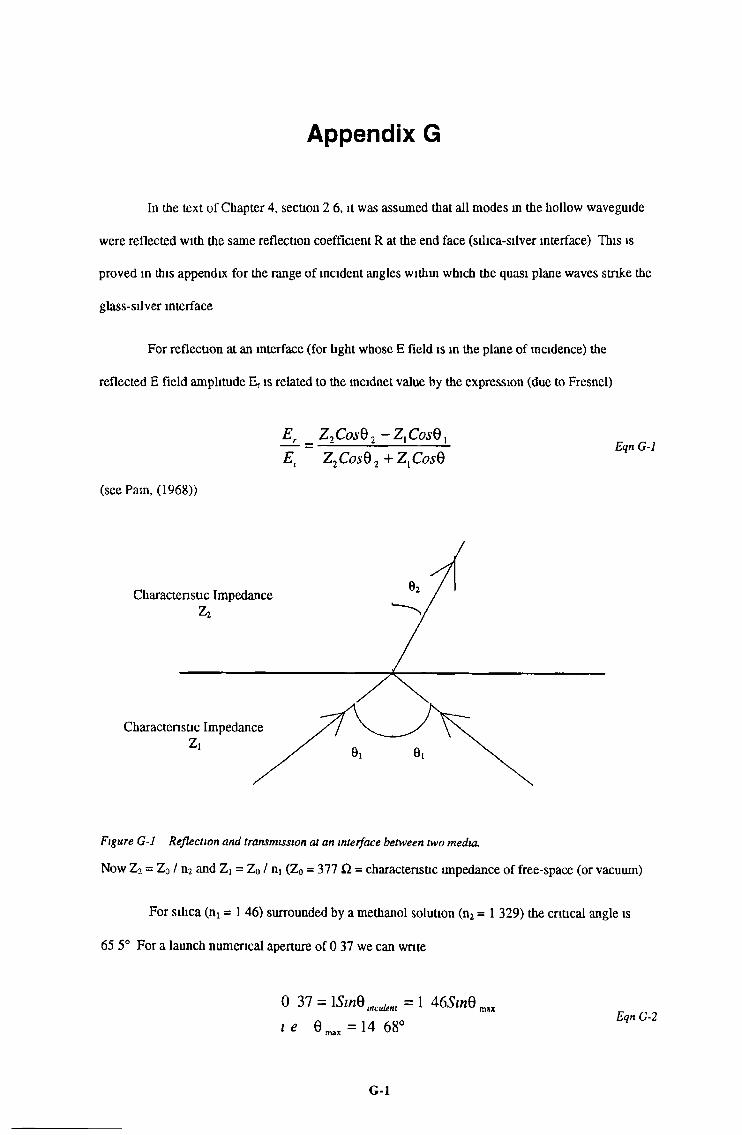
Appendix G
In the text of Chapter 4, section 2 6, it was assumed that all modes in the hollow waveguide
were reflected with the same reflection coefficient R at the end face (silica-silver interface) This is
proved in this appendix for the range of incident angles within which the quasi plane waves strike the
glass-silver interface
For reflection at an interface (for light whose E field is in the plane of incidence) the
reflected E field amplitude Er is related to the incidnet value by the expression (due to Fresnel)
Er Z2Cas0 2 - Z. Cas0,— = — ----- 1---- 1-------L Eqn G-lEx Z2Cos02 + Z {Cos6
(see Pam, (1968))
Figure G-l Reflection and transmission at an interface between two media.
Now Z2 = Zo / n2 and Zi = Z0 / n! (Z0 = 377 Ì2 = characteristic impedance of free-space (or vacuum)
For silica (ni = 1 46) surrounded by a methanol solution (n2 = 1 329) the critical angle is
65 5° For a launch numerical aperture of 0 37 we can write
.< 0 =14 68° *"0J
G-l
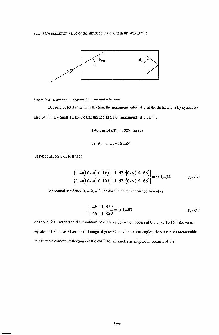
0max is the maximum value of the incident angle within the waveguide
Figure G-2 Light ray undergoing total internal reflection
Because of total internal reflection, the maximum value of 9, at the distal end is by symmetry
also 14 68° By Snell’s Law the transmitted angle 02 (maximum) is given by
1 46 Sin 14 68° = 1 329 sin (02)
1 e 02 (maximum) = 16 165
Using equation G-l, R is then
(1 46)[Co.v(l6 16)]-1 329[Co,(l4 68)] = q (1 46)[Cos(l6 16)]+1 329[Cay(l4 68)]
At normal incidence 0i = 02 = 0, the amplitude reflection coefficient is
1 4 6 - ! 329 = 0 0487
Eqn G-3
Eqn G-41 46+1 329or about 12% larger than the minimum possible value (which occurs at 0j (max) of 16 16°) shown in
equation G-3 above Over the full range of possible mode incident angles, then it is not unreasonable to assume a constant reflection coefficient R for all modes as adopted in equation 4 5 2
G-2
Appendix F References.Pam HJ “The Physics of Vibrations and Waves” (Wiley & Sons NY, 1968) Chapter 7, p208
G-3
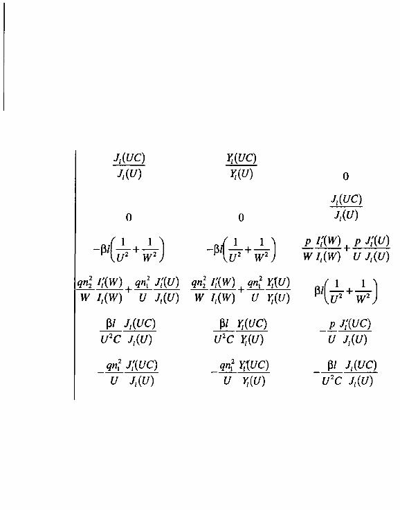
M u e )J,(U)
0
qn\ i;(W ) | qn\ J¡{U) W 7,(IV) U J,(U)
ß/ j,mU2C J,(U)
qn¡ J'AUC) U Jt{U)
Y<(UC)m
0
qnj m | qn\ Yt{U) W l,(W ) U Y,(U)
ß/ Y,{UC) U2C Y,(U)W YXUC) U Yt(U)
J,(UC)J,(U)
p m , p j;{u)W It(IV) U J,(U)
0
p jguc)U J,(U)
ß/ J,(UC)U2C J,(U)
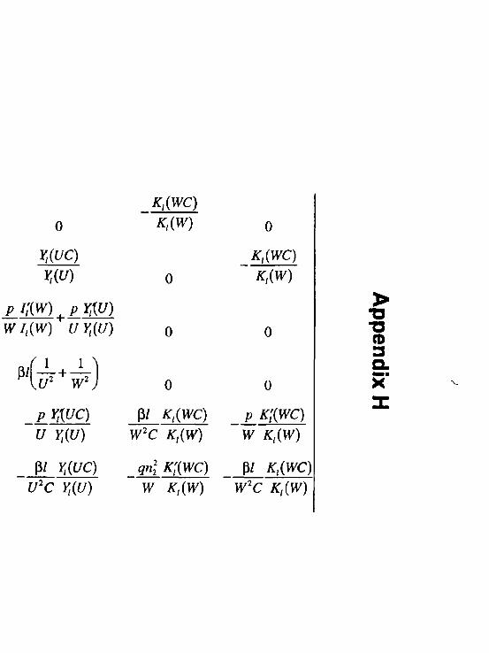
K,(WC)
Y,(UC)Y,(U)
p i; (w) | p YXU) W I,(W) U Yt(U)
0
P Y,{UC) U Y,(U)P/ Y,{UC)
U2C Yt{U)
K,(W )
0
0
0
p/ Kt{WC) W2C K,(W)
qnl K;(WC)
K,(WC)K,(W)
0
0
p k ;(w c )W K,(W)PI K,(WC)
0
W K,(W) W2C K,{W)
Appendix H


![Optical Surface Microtraps based on Evanescent Waves · Optical Surface Microtraps based on Evanescent Waves Dissertation zur Erlangung des Doktorgrades an der ... [Fol02]. While](https://img.pdfslide.us/doc/110x75/5bdee43809d3f2647f8b63e5/optical-surface-microtraps-based-on-evanescent-optical-surface-microtraps-based.jpg)