Embed Size (px)
Citation preview

1
NGWU JAPHET IFEANYI
PG/M.ENG/2007/42922
EVALUATION OF VIABILITY OF A CRUDE OIL RESERVOIR USING
PETROPHYSICAL PARAMETERS (A CASE STUDY OF AGBARA OIL
WELL RESERVOIR IN THE NIGER-DELTA BASIN)
Mechanical Engineering
A THESIS PRESENTED IN PARTIAL FULFILMENT OF THE REQUIREMENTS FOR THE AWARD OF DEGREE OF MASTER OF ENGINEERING (M.ENG) IN
MECHANICAL ENGINEERING.
Webmaster
2009
UNIVERSITY OF NIGERIA

2
EVALUATION OF VIABILITY OF A CRUDE OIL RESERVOIR
USING PETROPHYSICAL PARAMETERS
(A CASE STUDY OF AGBARA OIL WELL RESERVOIR IN
THE NIGER-DELTA BASIN)
BY
NGWU JAPHET IFEANYI
PG/M.ENG/2007/42922
DEPARTMENT OF MECHANICAL ENGINEERING
UNIVERSITY OF NIGERIA, NSUKKA
SUPERVISOR: PROF A.O.ODUKWE
NOVEMBER,2009
1
EVALUATION OF VIABILITY OF A CRUDE OIL
RESERVOIR USING PETROPHYSICAL PARAMETERS
(A CASE STUDY OF AGBARA OIL WELL RESERVOIR IN
THE NIGER-DELTA BASIN)
BY
NGWU JAPHET IFEANYI
PG/M.ENG/2007/42922
A THESIS PRESENTED IN PARTIAL FULFILMENT OF THE
REQUIREMENTS FOR THE AWARD OF DEGREE OF MASTER OF
ENGINEERING (M.ENG) IN MECHANICAL ENGINEERING.
DEPARTMENT OF MECHANICAL ENGINEERING
UNIVERSITY OF NIGERIA, NSUKKA
NOVEMBER,2009.

2
CERTIFICATION
Ngwu Japhet Ifeanyi, a post-graduate student in the department of
Mechanical Engineering, with registration number PG/M.ENG/2007/42922, has
satisfactorily completed the requirements for the course and research work of the
degree of master of engineering in mechanical engineering with option in Industrial
Engineering and Management.
The work embodied in this thesis is original and has not been submitted in
part or in full for any other diploma or degree of this or any other university.
_____________________ _______________________
Ngwu Japhet Ifeanyi Engr. Prof. A. O. Odukwe
Student Project Supervisor
Date…………………….. Date……………………….
_____________________ _______________________
Engr. Prof. S. O. Onyegegbu External Examiner
Head of Department Date………………………..
Date…………………

3
ACKNOWLEDGEMENTS
My sincere gratitude goes to the Almighty God for the enablement and guidance, for
he alone is the source of all knowledge in the mystery of the trinity.
Unique appreciation goes to my project supervisor, Prof. A. O. Odukwe, for the
excellent supervisory skills provided during the planning and review of every phase
of this work. My sincere thanks goes to my sub-supervisor, Engr. Dr. Stephen
Nwanya for his total commitment and guidance in actualizing this noble task.
I am deeply indebted to my immediate family members, especially my elder brother,
Mr. Clifford Emeka Ngwu, whom without his encouragement and financial support,
this work should have died in my mind.
I also wish to express my deep gratitude to the management and staff of Chevron
Nigeria Limited, and Schlumberger Nig Ltd, for their immense corporation given to
me, especially in obtaining their individual data.
Special thanks also goes to some of my postgraduate course mates for their
wonderful encouragements rendered to me at some difficult stages of this work.
It is my fervent hope that every reader of this work will be motivated to know the
most economical means of evaluating the viability of a crude oil reservoir.

4

5
ABSTRACT
This research work is aimed at determining the most economical means of estimating the
quantity of hydrocarbon saturations in a particular reservoir and the evaluation of oil ultimate
recovery using the recovery factor (RF) equations that have been developed. In order to
achieve this aim, a model called Area-depth concept model was developed using Agbara oil
well reservoir in Niger-Delta as a case study. This model is an extension of the existing
volumetric model which has been found insufficient in the evaluation of reservoir viability.
The method considers a reservoir as an enclosed volume element and to planimeter the
isopachous or horizon map drawn from a reservoir cross-section. The integral of the reservoir
volume was taken and the values of bulk gas sand volume, Vg, and bulk oil sand volume,
VO, were analytically estimated from the cumulative bulk volume plot (CBV plot). Using the
collected field data and the necessary related petro-physical parameters, the stock tank oil
initially in place (STOIIP) in the reservoir and the recoverable quantity were analytically
estimated from the CBV Plot. In this study, an evaluation of actual log readings from Niger-
Delta were collected and used to calculate the connate water saturations in order to determine
the productive oil zones in a reservoir by using Achie’s Equations. Equilibrium initialization
algorithm was also used to determine pressure gradient in a particular reservoir . The
research also covered the basic economic measures that are related to oil production.
Considering the related petrophysical parameters involved in the evaluation, the
reservoir was found to contain an oil deposit of 295.8 x 10⁶ stock tank barrel (stb).
The amount recovered for a case where there is a strong aquifer influx was 153.82 x
106 stb. The amount of recovery for a case where there is no aquifer influx was 136.1
x 106 stb. These results showed that the reservoir investigated was economically
viable. It is hoped that this study will be helpful for efficient, quick collection, processing
and interpretation of drilling data to analytically give the accurate estimation of recoverable
hydrocarbon in a particular reservoir in order to achieve optimum yield.

6
TABLE OF CONTENTS
Title page i
Approval page ii
Acknowledgement iii
Abstract iv
Table of contents v
List of figures viii
List of tables ix
List of symbols x
CHAPTER ONE
1.0 Introduction 1
1.1 Objectives of the Study 2
1.2 Significance of the Study 2
1.3 Limitations of the Study 2
1.4 Methodology 3
CHAPTER TWO
2.0 Literature Review 5
2.1 Background of the Study 5
2.2 Petrophysical Evaluation 9
CHAPTER THREE
3.0 Research Methodology 33
3.1 Area-Depth Concept Model 33
3.2 Modification of Formula for Estimation using Volumetric Method 36
3.3 Mathematical Analysis of Reservoir Geometry by Area-Depth
Concept Model using Horizon or Isopachous Map 36
3.4 Assumptions in the Application of Area –Depth Concept Model 38
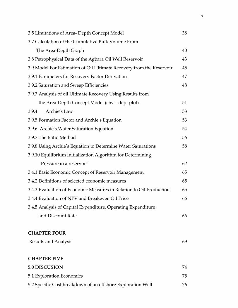
7
3.5 Limitations of Area- Depth Concept Model 38
3.7 Calculation of the Cumulative Bulk Volume From
The Area-Depth Graph 40
3.8 Petrophysical Data of the Agbara Oil Well Reservoir 43
3.9 Model For Estimation of Oil Ultimate Recovery from the Reservoir 45
3.9.1 Parameters for Recovery Factor Derivation 47
3.9.2 Saturation and Sweep Efficiencies 48
3.9.3 Analysis of oil Ultimate Recovery Using Results from
the Area-Depth Concept Model (cbv – dept plot) 51
3.9.4 Archie’s Law 53
3.9.5 Formation Factor and Archie’s Equation 53
3.9.6 Archie’s Water Saturation Equation 54
3.9.7 The Ratio Method 56
3.9.8 Using Archie’s Equation to Determine Water Saturations 58
3.9.10 Equilibrium Initialization Algorithm for Determining
Pressure in a reservoir 62
3.4.1 Basic Economic Concept of Reservoir Management 65
3.4.2 Definitions of selected economic measures 65
3.4.3 Evaluation of Economic Measures in Relation to Oil Production 65
3.4.4 Evaluation of NPV and Breakeven Oil Price 66
3.4.5 Analysis of Capital Expenditure, Operating Expenditure
and Discount Rate 66
CHAPTER FOUR
Results and Analysis 69
CHAPTER FIVE
5.0 DISCUSION 74
5.1 Exploration Economics 75
5.2 Specific Cost breakdown of an offshore Exploration Well 76

8
5.3 Analysis of the Economic viability of Agbara oil well reservoir
using the total cost expenditure 78
5.4 Formation Evaluation 78
5.5 Well Test Analysis 79
5.6 Importance of Well Test Analysis 80
5.7 Common Types of Reservoir 81
5.8 Application of Fluid Pressure To Determine Gas Oil Contact(GOC),
Gas Water Contact(GWC), Oil Water Contact(OWC) 82
5.9 Pressure and Temperature Gauge Placement 83
5.9.1 Gauge Performance Check 84
5.9.2 Pressure Programming and Interpretation for RFT Analysis 85
5.9.3 Laboratory Analysis of Oil Samples 86
CHAPTER SIX
6.0 Conclusion 87
6.1 Recommendations 88
References
Appendix

9
LIST OF FIGURES
Fig. 4.1. Disciplinary Contributions to Reservoir Flow Modeling 24
3.1 Horizon Map 36
3.2 Cross-Section of an Oil Reservoir 36
3.3 (A) Dome Shaped Structure of a Reservoir with
Top and Base Areas 37
(B) Plan View of a Reservoir Cross Section. 37
3.4: Area – Depth Graph 40
3.5: Cumulative Bulk Volume Plot 42
3.6 Initial Condition of a reservoir 46
3.7 Abandonment Condition of a Reservoir 46
3.8 Saturations and Sweep Efficiency 48
3.9: Data from Actual Log Readings Taken in the Niger-Delta 59
3.10 Depths for Initialization Algorithm 62

10
LIST OF TABLES
Table 2.1: Quick check sand and shale indicator 31
(Resistivity and Gamma Ray)
2.2 Measurement corrections 32
3.1 Values of top and bottom areas 39
3.2 Cumulative bulk volume plot 41

11
LIST OF SYMBOLS
gastheofsSaturationSg S
oiltheofsSaturationSo
F= Net- to – gross ratio
Boi = Initial oil formation volume factor
Ei = Initial gas expansion factor
Ew = Sweep efficiency to water drive
Ssw = connate water saturation
Eg = Sweep efficiency to gas drive
Sorw = Residual oil saturation to water drive
Sorg = Residual oil saturation to gas drive
Ha =Abandonment Oil Column,
= porosity,
Ct = electrical conductivity of the fluid saturated rock.
Cw = the brine saturation
m = Cementation exponent of the rock (usually in the range 1.8-2.0).
n = saturation exponent (usually close to 2).
Rt = Fluid saturated rock resistivity
Rw = the brine resistivity
Sw = fraction of pore volume occupied by water,
F = formation factor, a coefficient equal to the ratio of the resistivity of a 100%
saturated rock to the resistivity of the water solution contained in that rock
Rt = True resistivity of the un-invaded zone.
Rw= Resistivity of the formation water.
ℓ = Density
g = Acceleration due to gravity

12
h = Change in Height
i = Annual inflation rate
Q = Number of times interest is compounded each year
N = Number of years of the expenditure schedule
ΔE(k) = expenses incurred during a time period k
ΔNp(k) = incremental oil production during period k
ROR = Rate of Return
Pun = price per unit quantity produced during year n,
Qn = Quantity produced during year n
Po = present price of oil
)(kNo
p = incremental oil production during period K
rateoductionq Pr
tyPermeabiliK
ityVis cos
AreationalCrossA sec
gradientessureL
PPr
BVg =Gas flooded zone
BVw = Water flooded zone
BVo = Abandonment oil zone
Boa = Formation volume factor at abandonment condition
Vb = Bulk vo
typermeabiliAbsoluteK
oiltotypermeabiliEffectiveK
oiltotypermeabililativeK
o
ro
Re

13
SCFbblfactorvolumeformationgasInitialB
SCFgasreservoirInitialG
STBbblfactorvolumeformationOilB
STBoilproducedCumulativeN
STBbblfactorvolumeformationoilInitialB
STBoilreservoirInitialN
gi
o
p
oi
/,
,
/,
,
/,
,
bblwaterreservoirInitialW
SCFbblfactorvolumeformationGasB
STBSCFratiooilgasSolutionR
STBSCFratiooilgasproducedCumulativeR
STBSCFratiooilgassolutionInitialR
SCFreservoirtheingasfreeofAmountG
g
so
p
soi
f
,
/,
/,
/,
/,
,
1
1
,
,
,
,
,intinf
/,
,
PsiilitycompressibisothermalFormationC
bblspacevoidInitialV
saturationwaterInitialS
PsiapressurereservoiraverageinChangeP
PsiilitycompressibisothermalWaterC
bblreservoiroluxWaterW
STBbblfactorvolumeformationWaterB
STBwaterproducedCumulativeW
f
f
wi
w
e
w
p

14
CHAPTER ONE
1.0 INTRODUCTION
Generally, the major oil companies maintain their own research and
development (R&D) records and also, nurture in-house technological and
engineering skills acquisition schemes. For this reason, some companies see the core
activities needed before oil exploration as unrealistic if carried out, externally.
They now preserve only what is essential to evaluating the cost of exploration
from a particular reservoir.
These core activities include the formation evaluation technique, which is
applied to determine hydrocarbon saturation in a given reservoir, the determination
of oil- in- place (OIP) or stock Tank Oil initially in Place (STOIIP) and the application
of ultimate Recovery Factor (URF), based on analysis of some petrophysical
parameters using current technology.
This research work gives attention to determining the most economical means
of estimating the percentage of hydrocarbon saturation in a particular reservoir, and
its recovery factor. A model called, Area – Depth concept model was developed to
analytically estimate the quantity of crude oil deposits in a reservoir, using Agbara
oil well reservoir as a case study. The basic economic measures that are related to oil
production were evaluated. In this research, Archies’ Law was applied in the
determination of water saturations at different zones in a particular reservoirs based
on the log data of the petrophysical parameters from the Agbara oil well reservoir,
in the Niger-Delta basin. This helps to determine the productive oil zones by
estimating the percentage of hydrocarbon saturations in the reservoir. This study
would help reduce considerably the overall cost involved in executing recovery
process from a particular reservoir in order to achieve optimum yield.
There is no doubt in the fact that the world has consumed approximately 40
percent of the estimated recoverable reserves, i.e. more than one- third of the easily
recoverable reserves have been found and consumed (Stela Shamon,1998).

15
When 50 percent of recoverable reserve is reached, production will inevitably
go down because of the difficulty of extracting the rest. The only hope of extending
the world’s oil reserve is to make a quantum leap in production from 35% to 60%.
1.1 OBJECTIVES OF THE STUDY
1. To estimate the quantity of recoverable hydrocarbon in a reservoir and
evaluate the recovery factor, by using the related petrophysical parameters.
2. To improve the efficacy of volumetric method in reservoir evaluation by
using the area-depth concept model.
3. To determine the productive oil zones in a particular reservoir , by the use of
Archie’s equations.
4 To develop initialization algorithm for determination of
pressure gradient in a reservoir.
5 To evaluate the basic economic measures in relation to oil production.
1.2 SIGNIFICANCE OF THE STUDY
The significance of this research work will include:
Provision of a background for easy interpretation of resulting drilling data
before and during exploration.
Reduction in the overall drilling costs from a reservoir.
Improvement on the quality and quantity of crude oil recovered from a
particular reservoir
Reduction in the cost of energy to consumers
1.3 LIMITATIONS OF THE STUDY
1. First, it would be impossible within the short time frame of this study to
conduct extensive oral or written interviews outside Port Harcourt
2. Secondly, time factor would also not permit to deal exhaustively with the
issues of management views arising from the first constraint.
3. Thirdly, the values of the petrophysical parameters from log readings used
for these evaluations are only dependent upon the precision and accuracy of
the instrument used.

16
1.4 METHODOLOGY
The information for this study will be obtained from the following sources;
Publications such as: Learned journals ,Internet and Seminars.
Research findings from Schlumberger oil services Ltd and Chevron Nigeria Ltd, in
Port Harcourt.
Data collected from actual drill samples during fieldwork was used for the
analysis of formation evaluation. They were collated and analyzed. These data
include the petro-physical parameters like porosity, permeability, resistivity,
shaliness, lithology and formation temperature. These data would be used to
evaluate the viability of a reservoir, by the use of formation factor and Archie’s
Equation. Also, information on economic and management considerations would be
obtained from interviews and observations during a visit to some selected
companies in the Niger- Delta area.
The processes, economics and management of enhanced drilling techniques
are pre-requisite for the actualization of these objectives.
Formation evaluation (Otherwise referred to as log Interpretation) is the
process whereby physically measurable properties are translated into petrophysical
parameters of interest. Some of the major petro-physical parameters that would be
used in this research work, to determine and evaluate the viability of a crude oil
reservoirs are as follows:
Resistivity (R) :- The reluctance of a unit volume of formation (matrix + fluid)
to the flow of electrical current
Porosity (ø):- This is the percentage of void space in a unit volume of rock.
Hydrocarbon saturation (S): This is the percentage of pore space filled with
hydrocarbons (gas or oil).
Permeability (K):- This is the measure of the specific flow capacity or ease
with which fluid flows.
Lithology (L):- This is the study of rocks to determine their character and
composition

17
Shaliness (Vsh):- The fraction of a very fine grained detrital sedimentary rock
composed of silt and clay. It is the volume of shale in a particular rock
formation.
Water saturation (Sw)-: The percentage of the porous fraction of formation
that contains water.

18
CHAPTER TWO
2.0 LITERATURE REVIEW
2.1 BACKGROUND OF THE STUDY
The volumetric method for estimating oil in place is based on log and core analysis
data to determine the bulk volume, the porosity and the fluid saturations, and on
fluid analysis to determine the oil volume factor. Under initial condition 1 ac-ft of
bulk oil productive rock contains:
1.2)1(7758tan SwxxOilkStock
But for oil reservoirs under volumetric control there is no water influx to replace the
produced oil, so it must be replaced by gas, of which its saturation increases as the
oil saturation decreases. If Sg is the gas saturation and Bo is the oil formation volume
factor at abandonment conditions, then 1 a c-ft of bulk rock contains;
2.2
)1(7758tan
0
gw SSxxOilkStock
Where 7758 barrels is the equivalent of 1 ac-ft (Allan and Sun, 2003).
The volume element of a reservoir that is considered porous is called the rock
porosity and the fraction of the pore space that is occupied by connate water is
called the connate water saturation Swc. Hence the pore space filled by hydrocarbon
called the hydrocarbon pore volume (HCPV), is given by;
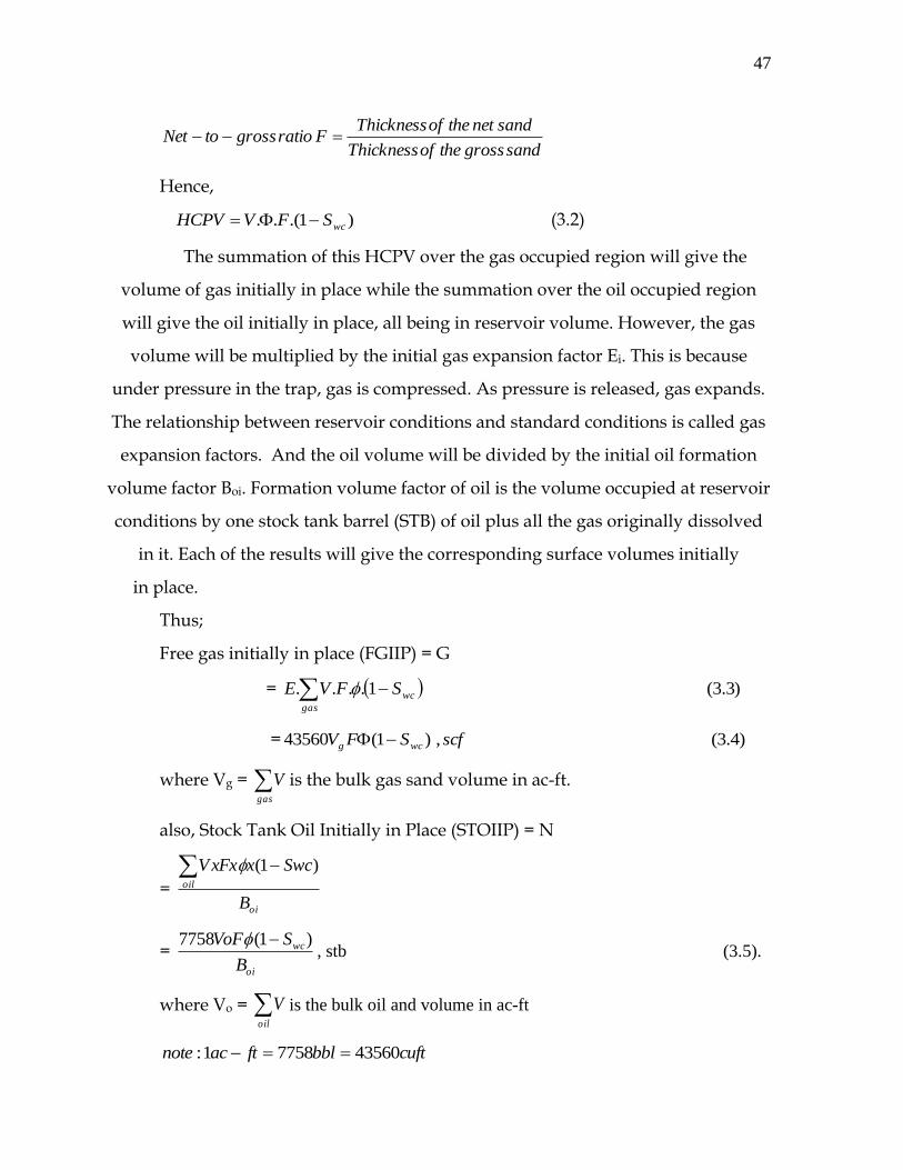
3.2)1( wcSxxVHCPV
The summation of the hydrocarbon pore volume over the gas occupied region will
give the volume of the gas initially in place while the summation over the oil region
will give the oil initially in place all being in reservoir volume (Green and Whillite,
1998). In a reservoir evaluation using the volumetric method, the reservoir system is
considered to be a container whose volume represents the quantity of oil in place.
The porosities and fluid saturation are obtained from core analysis.
For an oil system, there is an amount of water present from origin called connate
water. This is the water in the oil and gas bearing parts of a petroleum reservoir

19
above the transition zone. This water is important because it reduces the amount of
pore space available to oil and gas and it also affects their recovering. Connate water
is generally not uniformly distributed throughout the reservoir but varies with the
permeability and lithology. (Schlumberger Well Evaluation Conference, (SWEC),
1997).
Thus, the fluid saturation with the systems is given by:
.1.:
1
WCSS
SS
o
WCO
A volumetric balance states that since the volume of a reservoir (as defined
by its initial limits) is a constant, the algebraic sum of the volume changes of the oil,
free gas, water, and rock volumes in the reservoir must be zero(Everdingen et al,
1953). For example if both the oil and gas reservoir volumes decrease, the sum of
this two decreases must be balanced by changes, equal in magnitude to the water
and rock volumes.
The ratio of the initial gas cap volume to the initial oil volume, symbol is
given as: volumeoilreservoirInitial
m volumegas freereservoir initial
The value of m is determined from log and core data and from well completion data,
which frequently helps to locate the gas oil and water oil contacts. The ratio m is
known in many instances much more accurately than the absolute values of the gas
cap and the oil zone volume (Firroozabadi, 1996). In the evaluation of the reservoirs
that are produced simultaneously by the three major mechanisms of depletion drive,
segregation or gas cap drive and water drive, it is of practical interest to determine
the relative magnitude of each of these mechanisms that contribute to the
production of oil in the reservoir.
The principal problems in preparing the contour map are the proper
interpretation of net sand thickness from the well logs and the outlining of the
productive area of the field as defined by the fluid contacts, faults, or permeability
barriers on the subsurface contour map.
20
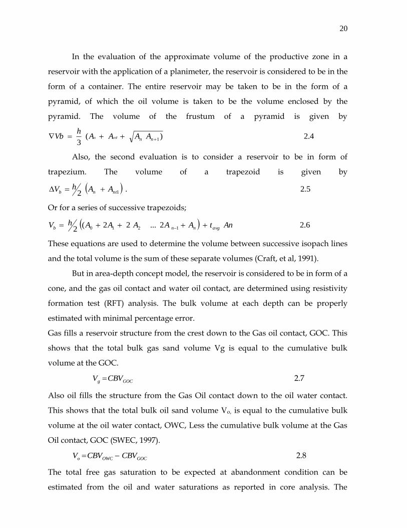
In the evaluation of the approximate volume of the productive zone in a
reservoir with the application of a planimeter, the reservoir is considered to be in the
form of a container. The entire reservoir may be taken to be in the form of a
pyramid, of which the oil volume is taken to be the volume enclosed by the
pyramid. The volume of the frustum of a pyramid is given by
4.2)(3
1 nn AAAAh
Vb ntIn
Also, the second evaluation is to consider a reservoir to be in form of
trapezium. The volume of a trapezoid is given by
5.2.2 1ntnb AAhV
Or for a series of successive trapezoids;
6.22...22(2 1210 AntAAAAAhV avgnnb
These equations are used to determine the volume between successive isopach lines
and the total volume is the sum of these separate volumes (Craft, et al, 1991).
But in area-depth concept model, the reservoir is considered to be in form of a
cone, and the gas oil contact and water oil contact, are determined using resistivity
formation test (RFT) analysis. The bulk volume at each depth can be properly
estimated with minimal percentage error.
Gas fills a reservoir structure from the crest down to the Gas oil contact, GOC. This
shows that the total bulk gas sand volume Vg is equal to the cumulative bulk
volume at the GOC.
GOCg CBVV 2.7
Also oil fills the structure from the Gas Oil contact down to the oil water contact.
This shows that the total bulk oil sand volume Vo, is equal to the cumulative bulk
volume at the oil water contact, OWC, Less the cumulative bulk volume at the Gas
Oil contact, GOC (SWEC, 1997).
GOCOWCo CBVCBVV 2.8
The total free gas saturation to be expected at abandonment condition can be
estimated from the oil and water saturations as reported in core analysis. The

21
expectation is based on the assumption that, while being removed from the well, the
core is subjected to fluid removal by the gas expansion liberated from the residual
oil. This process is somewhat similar to the depletion process in the reservoir.
In the case of reservoirs under hydraulic control, where there is no
appreciable decline in reservoir pressure, water influx is either inward and parallel
to the bedding planes as found in thin, relatively steep dipping beds (edge-water
drive), or upward where the producing oil zone (column) is underlain by water
(bottom water drive). Also, no free gas saturation develops in the oil zone and the
oil volume at abandonment remains the initial oil formation volume factor, Bo
(Green and Whilhite, 1998).
The above equations do not take into account the major petrophysical
parameters to be considered in the evaluation of ultimate recovery and recovery
factors. For example, the gas flooded zone, BVg, which consists of the gross bulk
volume for gas, sweep efficiency to gas drive, and the residual oil saturation to gas
drive. Water flooded zone, BVw, which consists of gross bulk volumes for water,
sweep efficiency to water drive and residual oil saturation to water drive.
Abandoned oil zone, BVa, which consist of the gross bulk volume to oil and the
abandonment oil column, Ha.
In petrophysics, Archie’s law relates the in-situ electrical conductivity of
sedimentary rock to its porosity and brine saturation.
)9.2(SCCm
ww
m
t
Reformulated for electrical resistivity, the equation reads;
10.2S
RR n
wm
wt
It is purely empirical law attempting to describe ion flow (mostly sodium and
chlorine) in clean, consolidated sands, with varying intergranular porosity. Electrical
conduction is assumed not to be present within the rock grains or in fluids other
than water.

22
To evaluate a physical formation, the parameters that are needed are its
porosity, hydrocarbon saturation, bed thickness, and permeability. Resistivity
measurement along with porosity and water resistivity allows to infer the water
saturation (Sw) of a formation’s pore space and thus to derive its hydrocarbon
content (1-Sw). (Frank Shray, 1997). The resistivity of a clean formation is
proportional to the brine with which it is fully saturated. The constant of
proportionality is called the formation resistivity factor, F. If Ro is the resistivity of a
non-shaly formation sample saturated with brine of resistivity, Rw, then
)11.2(w
o
R
RF
For a given porosity, the ratio w
o
R
Rremains nearly constant for all values of Rw
below about one ohm. However, the more the resistive waters, the value of F is
reduced as the Rw rises, and the grain size of the sand decreases. This phenomenon
is attributed to a greater proportionate influence of the surface conductance of the
grains in fresher waters. The formation factor is a function of the porosity, the pore
structure and pore size.(Archie, 1982). In a formation containing oil or gas the
resistivity is a function not only of the formation factor F, and water resistivity Rw,
but also of water saturation Sw.
2.2 PETROPHYSICAL EVALUATION
A Petrophysical evaluation of a reservoir requires the followings:
1. an estimate of the volume of hydrocarbons present and,
2. the rate at which they can be produced.
Volume of hydrocarbons present at any point in reservoir is dependent on porosity
(ø) (volume of pores between rock minerals) and fluid distribution within the pores.
Rate of production is dependent on permeability which is controlled by the
number, size and interconnection of pores.
2.3 POROSITY
This is the pore space available for hydrocarbon accumulation. Porosity, ø is defined
as the ratio of the void space in a rock formation to the bulk volume of the rock. It is

23
a measure of the space in a rock not occupied by the solid structure or framework of
the rock.
Mathematically,
p
p
VvolumeBulk
VvolumePorePorosity
,
, (2.12)
gp
p
VVolumeGrainVVolumePore
VVolumePore
,,
,
b
gb
b
p
V
VV
V
V )( (2.13)
Formulated in terms of densities:
)(
)(.:
fg
bgPorosity
(2.14)
Where ℓf = Density of the saturating fluid. Porosity measurement is necessary to
enable us identify lithology and calculate saturation water while or after drilling
(Allan and Sun,2003)
TYPES OF POROSITY
A). Primary porosity: This is sometimes called “original porosity” because it is an
inherent characteristic of the rock and established during initial deposition. It
is influenced by particle size, shape, sorting, packing and amount of
cementing. Sandstone, shale, chalks, crystalline rocks and oolitic limestone
generally have primary porosity. Primary porosity is responsible for almost
all economical accumulation of oil in sandstone.
B). Secondary Porosity: these results from various types of geological activities
that occur after sediment had been deposited. In this type of porosity, the
shape and size of the pores, their position in the rock and their mode of
interconnection bear no direct relation to the form of the sedimentary
particles. It may result from and be modified by solution, traction, fractures
and joints, recrystallization and dolomitization ,cementation and compaction.

24
Most of the reservoirs characterized by secondary porosity are composed of
carbonate rocks,(e.g. limestone and dolomite).
C) Absolute porosity: This is a measure of the total Pore spaces in a rock as a
function of the Bulk volume regardless of whether the pores are connected or
not. It is also called total porosity.
D) Effective porosity: A measure of the interconnected pore spaces as a function
of bulk volume. It is defined as the ratio of the volume of interconnected pore
space to the total bulk volume of the rock. It is this type of porosity that is
responsible for the migration of oil to well bore. Only this allows crude oil to
flow and be produced.
2.4 FORMATION VOLUME FACTOR FOR OIL, β0
Formation volume Factor of oil is the volume occupied at reservoir conditions
by one stock tank barrel (STB) of oil plus all the gas originally dissolved in it.
conditionsdardsatoilkstockofVolume
conditionsreservoiratgasdissolvedoilofVolumeO
tantan
Oil formation Volume Factor (FVF) is required for both reservoir and production
system calculations. The reservoir engineer must be able to relate stock tank
volumes to reservoir volumes at various pressures under constant reservoir
temperatures.
The volume of oil entering the stock tank at the surface is less than the
volume of oil which flows into the well bore from the reservoir.
The most important factor is the evolution of gas from the oil as pressure is
decreased from reservoir pressure to surface conditions. This causes a large decrease
in oil volume if there is a significant amount of dissolved gas.
Other minor changes include the expansion of the remaining oil due to
reduction in pressure. But this is somewhat offset by the contraction of the oil due to
the reduction in temperature.

25
2.5 TOTAL FORMATION VOLUME FACTOR
The total amount of gas produced at the surfaces can of course exceed the solutions
gas since, in addition to dissolved gas, some free gas may also be produced.
The produced gas ratio, R, may therefore be split into two components,
)( ss RRRR (2.15)
The first component, Rs Scf/STB is the solution gas oil ratio, GOR< which when
taken down to the reservoir with one STB of oil will dissolve in the oil at the
prevailing reservoir conditions to yield β0 reservoir with one STB of oil will dissolve
in the oil at the prevailing reservoir conditions to yield β0 reservoir barrels (RB or
res. bbL) of oil plus dissolved gas.
The second component, R- Rs, Scf/STB, is the free gas which when taken
down to the reservoir will occupy a volume of:
(R-Rs) Scf
BRRBx
STB
scf gsg
)( res.bbls (2.16)
:. The total reservoir ( underground) hydrocarbon with withdrawal associated with
one STB of oil is:
gsot BRRBB )( (1.17)
This is called the total formation volume factor, βt
2.6 PERMEABILITY
The permeability of a porous rock is a measure of its ability to transmit fluids. The
magnitude of this fluid- passing property known as permeability is related to the
number, size, shape and continuity of the pores within the rock. A medium of high
permeability will pass fluids with relative ease, while one of low permeability will
pass fluids with difficulty.
A darcy of permeability defined as one in which one centilitre of fluid of one
centipoise ( i.e the viscosity of water at 680F) would flow through a portion of sand
one centimeter in length and having one square centimeter of areas through which
to move if the pressure drop across the sand is one atmosphere.
Permeability is represented by the letter K, and it is usually measured in
millidarcies, md.

26
The permeabilities of hydrocarbon – bearing rocks like sandstone range from a few
millidarcies to several thousand millidarcies. Generally, a sandstone with
permeability lower than one millidarcies is considered to be a non- producer
( Craft, et al.,1991).
Base on experiments by a French engineer, Henry Darcy, permeability is the
constant K in the equation.
L
PKAq
(2.18)
TYPES OF PERMEABILITY
A. Absolute permeability: This is a measure of the Ease of flow of a single fluid
through the porous medium, K.
B. Effective permeability: This is the permeability of a rock to a particular fluid
in the presence of other fluids.
Relative Permeability: This is the ratio of Effective permeability to the Absolute permeability
K
KK
oro . (2.19)
2.7 ROCK COMPRESSIBILITY
Rock compressibility depends on its
- Grain compressibility, Cr and
- Pore compressibility, Cp and
The external bulk of the rock is subjected to constant overburden pressure which the
internal fluid pressure is gradually reduced.
Accordingly, the grains (rock matrix) expand causing a corresponding
reduction in pore space. More fluid would be expelled from the pore spaces than
would be expected from fluid expansion alone.
Rock compressibility also known as formation compressibility Cf may be
given as prf CCC (2.20)
Where Cr = rock grain compressibility and Cp = pore volume compressibility
From most petroleum reservoirs, the change in rock grain volume is much less than
the change in porosity .

27
Accordingly, Cf = Cp = -
dp
dv
v
1 (2.21)
Total compressibility, Ct, The compressibility of Rock and Fluids Together is Given
as ; fggwwoot CCSCSCSC (2.22)
The total compressibility ranges from 10-5 to 10-4 psi-1 for systems above the
bubble point pressure( Green and Wilhite,1998).
When the system drops below the bubble point, the compressibility increases as the
pressure drop
Rock compression affects
- rock matrix, Cr
- pore space, Cp
Formation compression Cf = Cr + cp O
:. Cf = C (2.23)
dp
dv
vv
dvC
10 (2.24)
2.8 DETERMINATION OF OIL –IN-PLACE
OIL- IN- PLACE (OIP): The oil – in- place is the total volume of oil accumulated in
the pores of the reservoir. It could be measure in Stock Tank Barrel, STB or Reservoir
Barrels, RB.
The methods for determination of oil- in- place are:
1 Volumetric method (2) Material Balance method (3) Simulation modeling and (4)
decline curve Analysis method.
2.9 VOLUMETRIC METHOD OF ESTIMATING INITIAL OIL IN PLACE IN
RESERVOIR
The method considers a reservoir system to be a container whose volume
represents the quantity of oil in place. If there is a reservoir with a given porosity ,
then the volume of oil, water and gas in the system is given by:
sg
sw
o
volumeunitporosityGas
volumeunitporosityWater
SvolumeunitporosityOil
)(
)(
)(

28
The porosities and fluid saturations are obtained from core analysis. The area extent
of the reservoir is measured in Acre and the oil column is measured in Feet.
Hence from dimensional analysis, initial oil in place,
= 3615.5
343560
ft
Ibbl
ftacreI
ftXXso
3615.57758
ft
bbiso Xplaceinoilinitial
If the reservoir area is A acres and the oil column is lft, then the initial oil is
place in given by:
Initial oil in place =ftacre
bblftxacrexAxh so
7758
=> Initial oil in place = bblAh so7758 (2.25)
#For an oil system, there is an amount of water present from origin called connate
water. This is the water in the oil- and gas bearing parts of a petroleum reservoir
above the transition zone. It is also called interstitial water. Connate water is
important primarily because it reduces the amount of pore space available to oil and
gas and it also affects their recovering. Connate water is generally not uniformly
distributed throughout the reservoir but varies with the permeability and lithology.
(Schlumberger Well Evaluation Conference,(SWEC),1997).
Thus, the fluid saturation within the system is given by:
1 weo SS (2.26)
:. weo SS 1
Thus initial oil in place is given by;
Initial oil in place= stbShA we)1(7758 (2.27)
Bringing this quantity down to atmospheric condition, we have that the
hydrocarbon in place, which is commonly called the Stock Tank Oil Initially In Place
(STOIIP) is given as:
stbB
SwhASTOIIP
o
)1(7758 (2.28)
Refer To Appendix B for Conversions

29
2.9.1 MATERIAL BALANCE METHOD FOR ESTIMATION OF CRUDE OIL
RESERVE IN A RESERVOIR
The Material Balance Equation, MBE, is the balancing of inventory such as rig
platforms and other rig facilities in the reservoir. The general MBE is of the form:
TOTAL PRODUCTION = TOTAL EXPANSION
The general material balance equation is simply a volumetric balance, which
states that since the volume of a reservoir (as defined by its initial limits) is a
constant, the algebraic sum of the volume changes of the oil, free gas, water, and
rock volumes in the reservoir must be zero (Everdingen, Timmerman and
McMahon,1953). For example, if both the oil and gas reservoir volumes decrease, the
sum of these two decreases must be balanced by changes equal in magnitude to the
water and rock volumes. If the assumption is made that complete equilibrium is
attained at all times in the reservoir between the oil and its solution gas, it is possible
to write a generalized material balance expression relating the quantities of oil, gas
and water produced, the average reservoir pressure, the quantity of water that may
have encroached from the aquifer, and finally the initial oil and gas content of the
reservoir. In developing this mathematical model, the following production,
reservoir and laboratory data are involved.
1. The initial reservoir pressure and the average reservoir pressure at successive
intervals after the start of production.
2. The stock tank barrels of oil produced, at any time or during any production
interval.
3. The total standard cubic feet of gas produced.
When gas is injected into the reservoir, this will be the difference between the total
gas produced and that returned to the reservoir.
4. The ratio of the initial gas cap volume to the initial oil volume, symbol m.
volumeoilreservoirInitial
volumegasfreereservoirInitialm

30
If this value can be determined with reasonable precision, there is only one
unknown (N) in the material balance on volumetric gas cap reservoirs, and two (N
and We) in water-drive reservoirs. The value of m is determined from log and core
data and from well completion data, which frequently helps to locate the gas-oil and
water oil contacts. The ratio in is known in many instances much more accurately
than the absolute values of the gas cap and oil zone volumes(Firoozabadi,1996).
5. The gas the oil volume factors and the solution gas-oil ratios. These are
obtained as functions of pressure by laboratory measurements on bottom-hole
samples by the differential and flash liberation methods.
6. The quantity of water that has been produced.
7. The quantity of water that has been encroached into the reservoir from the
aquifer.
For simplicity, the derivation is divided into the changes in the oil, gas, water,
and rock volumes that occur between the start of production any time t. the change
in the rock volume is expressed as a change in the void space volume, which is
simply the negative of the change in the rock volume. In the development of the
general material balance equation, the following terms are used:
CHANGE IN THE OIL VOLUME
Initial reservoir oil volume = oiNB
Oil volume at time, t, and pressure, op BNNP )( (2.29)
change in oil volume = opoi BNNNB )( (2.30)
CHANCE IN FREE GAS VOLUME
NBoi
GBgim
volumeoilinitialto
gasfreeinitialofRatio
Initial free gas volume = GBgi = NmBoi (2.31)
solutionin
remainingSCF
produced
gasSCF
produced
gasSCF
dissolvedandfree
gasinitialSCF
tatgas
freeSCF ,

31
]SOSoi RNpCNRpNpNRBgi
NmBoiGf
(2.32)
BgNpNRpNpBgi
NmBoi
ttimeatvolumegas
freeservoirRNR SOiSOi
Re
BgNpNRpNpBgi
NmBoiNmBoi
volumegasfree
inChangeRNR SOSOi
(2.33)
CHANGE IN WATER VOLUME
pwwBwPwwBwww
cwpwecwpwevolumewater
inChange
e
(2.34)
CHANGE IN THE VOID SPACE VOLUME
Initial void space volume = Vf
)35.2(PCVPCVVV ffffffvolumespace
voidinChange
Or, because the change in void space volume is the negative of the
change in rock volume:
)36.2(PCV ffvolumerock
voidinChange
Combing the changes in water and rock volumes into a single, term, yields the
following:
i.e. change in water volume + change in rock volume
PCVPWWBW ffcwpwe
Recognizing that Swi
NmBoiNBoifthatandwifW VSV
1and by substitution,
then:

32
Change in water volume + change in rock volume
Pfwiw
wi
oioipwe
cscS
NmBNBWBW
1
)37.2(
11 P
wi
fwiwoipwe
s
cscNBmWBW
Equating the changes in the oil and free gas volumes to the negative of the changes
in the water and rock volumes and expanding all terms,
NpBgRsoNBgRsoNpRpBg
NRsoiBgBgi
NmBoiBgNmBoiNpBoNBoNBoi
)38.2(
11 P
wi
fwiwoipwe
s
cscNBmWBW
Now, adding and subtracting the term soigp RBN then;
gppsoi
gi
goi
oiopooiBRNBgNR
B
BNmBNmBBNNBNB
soigpsoigpsogpsog RBNRBNRBNRNB
)39.2(P
wi
fwiwsoippwe
sI
cscRNmIWBW
Then grouping the terms:
gsosoiopgsosoioooioi BRRBNBRRBBNNmBNB (
)40.2(PsI
cscNBmIWBW
B
BNmBNBRR
wi
fwiw
oipwe
gi
goi
pgsoip

33
Now writing tgsosoiotitioi BBRRBandBBB where Bt is
the two phase formation volume factor, as defined by the equation,
sooigot RRBBB
gi
g
tigoiptpttiB
BINmBBRRBNBBN
)41.2(PsI
cscBNmIWBW
wi
fwiwtipwe
This equation is the general volumetric material balance equation. ( Green and
Wilhite,1998).
It can be rearranged into the following form that is useful:
PsI
cscBNmIBB
B
NmBBBN
wi
fwiw
tigig
gi
titit
)42.2(pwgsoipppe WBBRRBNW
Each term on the left-hand side of equation 2.42 accounts for a method of
fluid production, and each term on the right-hand side represents an amount of
hydrocarbon or water production. The first two terms on the left-hand side account
for the expansion of any oil and/or gas zones that might be present. The term
accounts for the change in void space, which is the expansion of the formation and
cannot water. The fourth term is the amount of water influx that has occurred into
the reservoir. On the right-hand side, the first term represents the production of oil
and gas and the second term represent the water production. The mathematical
model by material balance method can be arranged to apply to any of the different
types of reservoirs.
For example, in an undersaturated oil reservoir, m=o, and thus, equation
(2.42), reduces to:
e
wi
fwiw
titit WPsI
cscBNBBN

34
pwgsoiptp WBBRRBN (2.43)
For gas reservoirs, equation 2.42, can be modified by recognizing that
gitippp GBNmBthatandGRN and substituting these terms into
equation (2.43), then:
ewiSI
fCwiSwC
gitigigtit WPGBNBBBGBBN
pwgoiptp WBBNRGBN (2.44)
When working with gas reservoirs, there is no initial oil amount, therefore, N and
Np are equal to zero. Therefore, the general material balance equation for a gas
reservoir can be obtained as the form;
pwgpewiSI
fCwiSwC
gigigWBBGWPGBBBG
(2.45)
In the study of reservoirs that are produced simultaneously by the three
major mechanisms of depletion drive, segregation or gas cap drive and water drive,
it is of practical interest to determine the relative magnitude of each of these
mechanisms that contribute to the production. Pirson(1958), rearranged the material
balance equation (2.42), to obtain three fractions whose sum in one. That is, the
Depletion Drive Index (DDI), the Segregation Drive Index (SDI), and the Water-
Drive Index (WDI) ( Pirson,1958).
When all the three drive mechanisms are contributing to the production of oil
and gas from the reservoirs, the compressibility term in equation 2.45, is negligible
and can be ignored. Moving the water production term to the left-hand side of the
equation, the following is obtained:
pwegiggiB
tiBmN
tit WBWBBBBN
p
gsoiptp BRRBN
Dividing through by the term on the right hand side of the equation:

35
gsoiptp
giggiB
tiNmB
gBsoiRpRtBpNtiBtBN
BRRBN
BB
46.21
gBsoiRpRtBpN
pWwBeW
The numerators of these three fractions that result on the left hand side of
equation (2.46) are the expansion of the initial oil zone, the expansion of the initial
gas zone, and the net water influx, respectively. The common denominator is the
reservoir volume of the cumulative gas and oil production expressed at the lower
pressure, which evidently equals the sum of the gas and oil zone expansions plus
the net water influx, then using the abbreviations of Prof. Pirson:
1 WDISDIDDI (2.47)
Finally, the general schilthwise material balance equation (2.42), can be
rearranged and solved for N, the initial oil in place:
PwiSI
fCwiSwC
tiBmIgiBgBgiBtimB
tiBtB
pWwBeWgBsoiRpRtBpN
N
(2.48)
If the expansion term due to the compressibilitie’s of the formation and
connate water can be neglected, as they usually are in a saturated reservoir, then
equation 2.48 becomes:
giBgBgiBtimB
tiBtB
pWwBeWgBsoiRpRtBpN
N
(2.49)
2.9.2 ADVANTAGES OF APPLYING MATERIAL BALANCE METHOD FOR
ESTIMATION OF OIL IN A RESERVOIR
1. Determination of initial oil in place
2. Calculation of water influx
3. Calculation of fluid contact movement
4. Prediction of the future recoveries

36
5. Prediction of reservoir pressures
6. Prediction of effect of production rate and/or injection rate (gas or water) on
reservoir pressure
7. Aquifer match of historical production leads to performance prediction.
2.9.3 RESERVOIR SIMULATION MODEL
Modern reservoir simulators are computer programs that are designed to
model fluid flow in porous media. Applied reservoir simulation is the use of these
programs to solve reservoir flow problem.
Modern reservoir management is generally defined as a continuous process
that optimizes the interaction between data and decision making during the life
cycle of a field. More specifically, reservoir management of hydrocarbon reservoirs
is defined as the allocation of resources to optimize hydrocarbon recovery from a
reservoir while minimizing capital investments and operating expenses
(Firoozabadi,1996). The primary objective in a reservoir management study of
hydrocarbon reservoir is to determine the optimum conditions needed to maximize
the economic recovery of hydrocarbons from a prudently operated field.
2.9.4 REASON FOR RESERVOIR SIMULATION
1. Corporate impact
Cash flow prediction
Need economic forecast of hydrocarbon price
2. Reservoir Management
Coordinate Reservoir management activities
Evaluate project performance
Interpret/ understand Reservoir behavior
Model sensitivity to estimated Data
Determine need for additional data
Estimate project life
Predict Recovery versus time
Compare different recovery processes

37
Plan Development or operational changes
Maximize Economic recovery
2.9.5 CONSENSUS MODELLING
This is the application of a computer simulation to the description of fluid flow in a
reservoir. The computer simulator, and the input data set is called the reservoir flow
model.
Many different disciplines contribute to the preparation of the input data set
of a flow model. The information is integrated during the reservoir flow modeling
process, and the concept of the reservoir is qualified in the reservoir simulator.
Fig 2.1 Disciplinary contributions to reservoir flow modeling
(Haldorsen and Damsleth, 1993).
Refer to Appendix C for planning of reservoir simulation
Seismic Petrophyscis Fluid
Properties
Geological
model
Numerical
Simulation
Model
Wells
Wells
Calibration of observations and production
data interpretations
Facilities
Model GRID
Effects

38
2.9.6 ESTIMATION OF OIL RESERVE IN A RESERVOIR USING DECLINE
CURVE ANALYSIS
The relationship between flow rate and time for producing wells assuming constant
flowing pressure, is found as;
1 n
t
qaq
d
d (2.50)
where a and n are empirically determined constants. The empirical constant n
ranges from 0 to 1(Arps, 1945).
Solutions to E.g. (2.50) shows the expected declined in flow rate as the production
time increase. Fitting an equation of the form of Eq (2.50) to flow rate data is
referred to as decline curve analysis. Three decline curves have been identified
based on the value of n.
the exponential decline curve corresponds to n= o. It has the solution
at
ieqq (2.51)
Where qi is initial rate and a is a factor that is determined by fitting Eq (2.51) to well
or field data.
The hyperbolic decline curve corresponds to a value of n in the range 0 < n< 1. The
rate solution has the form.
n
i
n qnatq (2.52)
where qi is initial rate and a is a factor that is determined by fitting Eq (2.52) to well
or field data.
The harmonic decline curve corresponds to n = 1. The rate solution is equivalent to
Eq (2.52) with n= 1, thus;
11 iqnatq (2.53)
where qi is initial rate and a is a factor that is determined by fitting Eq (2.53) to well
or field data.
Decline curves are fit to actual data by plotting the logarithm of observed rates
versus time t. The semilog plot yields the following equation for exponential decline:
atqq i lnln (2.54)

39
Eq (2.54) has the form bmxy , for a straight line with slope m and intercept b. In
the case of exponential decline, time t corresponds to the independent variable x, lnq
corresponds to the dependent variable y, Inqi is the intercept b, and – a is the slope
m of the straight line. Cumulative production for decline curve analysis is the
integral of the rate from the initial rate qi at time t = 0 to the rate q at time t.
For example, the cumulative production of oil in a reservoir, Np, for the
exponential decline case is given as:
t
itp
a
qqqdN
0 (2.55)
The decline factor a is for the exponential decline case and is found by rearranging
Eq (2.55)
Thus:itq
qa
ln1 (2.56)
2.9.7 RECOVERY FACTORS (RF)
The Recovery factor is the fraction of the Hydrocarbon initially in place (HCIIP), that
is deemed recoverable. Thus:
)57.2()( RFHCIIPURRECOVERYULTIMATE
The recovery factor is dependent on reservoir/ hydrocarbon characteristics,
recovery method, operating conditions and economics
( Schlumberger Well Evaluation Conference, 1997)
1. Reservoir characteristics as they affect RF
(a) Hydrocarbon column: This is the initial vertical distance between the
shallowest and deepest hydrocarbon points in the structure. At
abandonment, a certain minimum column will be left behind. This is called
the abandonment column. Ha. This is because a finite thickness of
hydrocarbon column must exist in the reservoir for the hydrocarbon to flow
into the producing well. This minimum depends on the type of well and
whether or not there is simultaneous presence of water and gas in the case of
an oil reservoir. The smaller the abandonment column, the higher the
recovery factor.

40
Other reservoir characteristics which affect recovery factor are:
(a) Presence or absence of gas
(b) Aquifer strength
(c) Residual saturations
(d) Permeability
(e) Heterogeneity
(f) Initial Reservoir pressure
Hydrocarbon characteristics as they affect RF
a) Viscosity
b) Density
c) Gas oil Ratio, GOR
2.9.7 RECOVERY FACTORS (RF)
There are different types of Recovery method which are normally applied during
exploration process. The method to be adopted depends on the nature of the
reservoir.
Primary recovery method: In primary oil recovery method, the recovery factor is
dependent on the natural reservoir energy. These are mainly the strength of aquifer
support and gas cap drive available. In the absence of these, the only energy
available would be due to the dissolved gas (solution gas drive) and reservoir
compaction. Both of these would usually result in recovery factors less than 10%.
However, the presence of a strong aquifer support or gas cap drive could lead to
recovery factors of 30 to 60%(Roman Talamantaz,1996).
ECONOMICS
The economic factors that affect Recovery Factor are:
- Location: The location of a hydrocarbon field affects the recovery
factor as the cost of production from certain remote areas will make
the production of certain volumes uneconomical while the same
volumes in a favourable location will have a non zero recovery factor.
- Price: This determines to a large extent not only the cut off for volumes
to be developed but also the cut off oil rate that can be allowed. Both of

41
these impact on the amount of oil that can be recovered and hence on
the recovery factor.
2.9.8 OPERATING CONDITIONS
The operating conditions that affect the recovery factor are:
- Government Regulations: These include minimum well spacing
requirements, duration of license and abandonment policy. All these
impact on the recovery factor.
- Environmental Regulations: This mainly affects disposable water
quality and gas fanning rules. The more stringent these regulations,
the lower the recovery factor.
- Overhead/operating cost: This affects the economic cut off oil rate. The
lower the operating cost, the lower the cut off oil rate and hence the
higher the recovery factors.
2.9.9 FORMATION EVALUATION
Until the drill bit penetrates the formation through the process of drilling a well, the
presence of petroleum in any formation remains unknown. At best, our geologists
and geophysicists can only suggest a probable structure (spot) where petroleum is
thought to exist. In the oil industry, there are methods the petroleum engineer
employs to locate and determine the quantity of petroleum in formation. In
addition, the evaluation and analysis of the information from the methods also
enable the petroleum engineer to determine and design the most efficient
programme to deplete the reservoir. The use and interpretation of these methods
and information provided by them is referred to as formation evaluation. The sole
objective of formation evaluation is to determine hydrocarbon saturation in a given
reservoir. Different formation Evaluation techniques are applied during the course
of well completion with the sole purpose of achieving one or more of the followings:
1. Identify a potential pay zone – by well log and core analysis.
2. The formation properties such as porosity, permeability and
fluid saturation – By well log and core analysis.
3. The fluid type – By well log, core log and well testing.

42
2.9.10 QUALITATIVE METHOD IN FORMATION EVALUATION
The first step in log interpretation should be to become familiar with the overall
aspects of the log in order to determine which areas are potential zones of interest.
This is done best through qualitative log interpretation.
To do this, the log analyst must try to gather information about typical
responses in the area being drilled. By knowing what tool responses are expected for
various lithologies, it is possible to view the log quite quickly and identify possible
areas of interest which can then be scrutinized more closely.
The log analyst should have in mind some criteria based on experience that
will allow him to identify the zones of interest and to divide the log into zones
which can be used for more detailed scrutiny (typically these will be hydrocarbon
and water bearing sands).
The resistivity of any formation is a function of the fluid type present in the
pore spaces of the matrix. Resistivity is mainly the function of the amount of water
in that formation and the resistivity of the water itself. Salt water is conductive,
while the rock grains and fresh water usually have very low conductivities. In the
Niger-Delta, saline water usually has a resistivity of 0.6 to 2 ohmm, depending on
the concentration of ions and the presence of hydrocarbons. Fresh water is not
common at depths more than 4000ft True Vertical Depth(TVD) and a resistivity
greater than approximately 3 ohmm may indicate a potential hydrocarbon-bearing
zone( Baker,1996).
Gamma ray baselines in the area are usually around 100 – 120 API and any
gamma ray drop below 65% of the shale baseline is generally a good indication of a
sand. Obviously, the cut-off value of the criteria may vary depending on the local
conditions and expected lithologies.
The combination of resistivity, gamma-ray neutron porosity, and rotational
density give a good indication of lithology, except in the presence of a gas. Tight
limestone is characterized by the density overlying the neutron porosity, with
Maximum Rotational Density (ROMT) = 2.71 g/cm3 and Thermal Neutron Porosity
(TNPH) = 0 (the tool is calibrated to match a water filled limestone). A tight
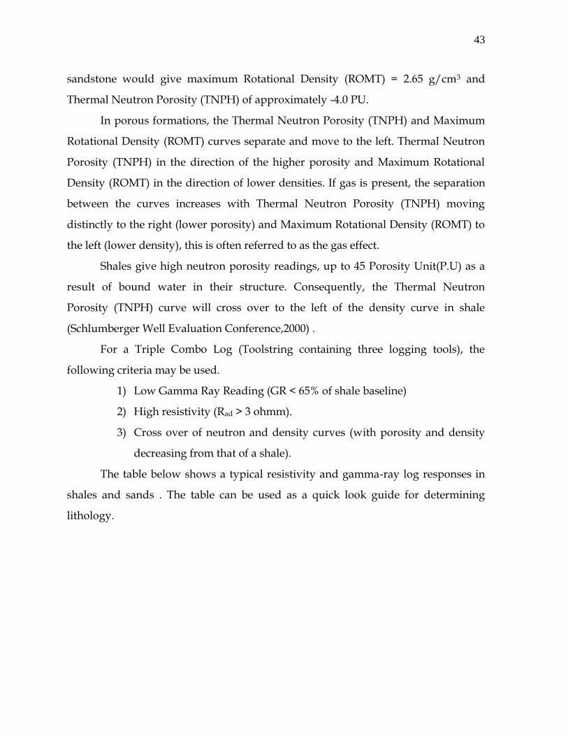
43
sandstone would give maximum Rotational Density (ROMT) = 2.65 g/cm3 and
Thermal Neutron Porosity (TNPH) of approximately -4.0 PU.
In porous formations, the Thermal Neutron Porosity (TNPH) and Maximum
Rotational Density (ROMT) curves separate and move to the left. Thermal Neutron
Porosity (TNPH) in the direction of the higher porosity and Maximum Rotational
Density (ROMT) in the direction of lower densities. If gas is present, the separation
between the curves increases with Thermal Neutron Porosity (TNPH) moving
distinctly to the right (lower porosity) and Maximum Rotational Density (ROMT) to
the left (lower density), this is often referred to as the gas effect.
Shales give high neutron porosity readings, up to 45 Porosity Unit(P.U) as a
result of bound water in their structure. Consequently, the Thermal Neutron
Porosity (TNPH) curve will cross over to the left of the density curve in shale
(Schlumberger Well Evaluation Conference,2000) .
For a Triple Combo Log (Toolstring containing three logging tools), the
following criteria may be used.
1) Low Gamma Ray Reading (GR < 65% of shale baseline)
2) High resistivity (Rad > 3 ohmm).
3) Cross over of neutron and density curves (with porosity and density
decreasing from that of a shale).
The table below shows a typical resistivity and gamma-ray log responses in
shales and sands . The table can be used as a quick look guide for determining
lithology.

44
Table 2.1: Quick Check Sand and Shale Indicator (Resistivity and Gamma Ray).
FORMATION AND
FLUID TYPE
CURVES COMMENTS
Shale Generally low resistivity and
high gamma ray counts
Gas filled clean sand Usually very high resistivity.
Low gamma ray counts
Oil filled clean sand Usually high resistivity low
gamma ray counts
Fresh water filled clean
sand
Usually high resistivity. Low
gamma ray counts
Salt water filled clean
sand
Usually low resistivity. Low
gamma ray counts
Fresh water filled silty
sand
Usually high resistivity. Low
gamma ray counts
Radioactive fresh water,
Gas or oil filled sand
Elevated gamma ray counts.
High resistivity.
KEY: Gamma Ray Curve (GR): (), Reistivity Curve (RES): ( )
Special notes: Possible pay sands or zones of interest generally have high resistivity
and low gamma ray. It is difficult to distinguish between fresh water, oil and gas
filled sands with resistivity and gamma ray only. It is therefore useful to consider
porosity and density to solve this problem. Shaly sands tend to have elevated
gamma ray counts and may be difficult to spot at first glance. Radioactive sands
have high gamma ray counts and may appear similar to shales, a spectral gamma
ray tool is advised if these type of sands are expected.
2.9.14 QUANTITATIVE METHODS
The data usually presented on final logs for client are usually corrected for
borehole effects, so that the measurements more accurately represent the physical
properties of the formation. The usual correction that apply up to this point are
shown below.

45
TABLE 2.2 MEASUREMENT CORRECTIONS
Measurement Symbol Corrections applied
Gammay Ray GR Hole size (bit), tool size, mud
weight
Attenuation Deep Resistivity Rad Borehole Compensated
Phase Shallow Resistivity Rps Borehole compensated
Thermal Neutron Density TNPH Hole size (bit), tool size,
borehole salinity, formation
salinity, matrix type, mud
hydrogen index
Bulk density RHOB Spine and ribs correction
Maximum Rotational
Density
ROMT Spine and ribs correction
SOURCE: Adaptation from “People and Technology”; A Directional Drilling
Training manual by Schlumberger.
At this point, a qualitative analysis is performed (as described in the previous
section) to determine the general properties of the log. Once the log has been
divided into zones by the qualitative analysis and the engineer has identified the
areas of interest, it is possible to undertake a more thorough and detailed numeric
analysis of the data (Texier and Alger,1965).
Several steps are usually taken to improve the accuracy of the data and to
employ empirical or theoretical relationships to the measured parameters to come
up with useful results which can be used to assess the potential of hydrocarbon
recovery from the formation. The steps that are taken usually involve determining
the quantity of hydrocarbon present in the formation and the economic viability of
producing it. Three other important economic factors usually considered before
embarking on production of hydrocarbon from a given reservoir include;
1) Estimation of the quality of recoverable hydrocarbon in the reserviour
2) Estimation of the recovery factor
3) And the evaluation of the financial potential of producing the reservoir

46
CHAPTER THREE
3.0 RESEARCH METHODOLOGY AND DATA ORGANIZATION
3.1 AREA-DEPTH CONCEPT MODEL
This model is developed in order to improve the efficacy of the volumetric
method in reservoir evaluations. Area-Depth concept involves a mathematical
analysis of the reservoir geometry. It uses subsurface and isopachous (horizon) map
based on the data from the electric logs, cores, drill stem and production tests. A
subsurface contour map shows lines connecting points of equal elevations on the top
of a marker bed and therefore shows geologic structure. The engineer uses this map
to determine the bulk productive volume of the reservoir. The volume is obtained
by planimetering the areas between the isopach lines of the entire reservoir or of the
individual units under consideration.
3.2 MODIFICATION OF FORMULA FOR ESTIMATION USING VOLUMETRIC
METHOD
The fraction of the volume element V that is porous is called the rock porosity
ø, and the fraction of the pore space that is occupied by connate water is called the
connate water saturation, Swc.
wcgwcg SSSS 11
Also, 1 wco SS
wco SS 1
Therefore, the saturations of gas or oil in any of the regions in a reservoir is given by
the factor , )1( wcS
Hence, the pore space that is filled by hydrocarbon (Called the Hydrocarbon
Pore Volume (HCPV) is;
)1.(. wcSVHCPV (3.1)
But in practice, there may be some parts of the sand that are not porous and
are discounted with what is called the net-to-gross ratio F where F is the fraction of
the total sand volume that is considered to be porous.
47
sandgrosstheofThickness
sandnettheofThicknessFratiogrosstoNet
Hence,
)1.(.. wcSFVHCPV (3.2)
The summation of this HCPV over the gas occupied region will give the
volume of gas initially in place while the summation over the oil occupied region
will give the oil initially in place, all being in reservoir volume. However, the gas
volume will be multiplied by the initial gas expansion factor Ei. This is because
under pressure in the trap, gas is compressed. As pressure is released, gas expands.
The relationship between reservoir conditions and standard conditions is called gas
expansion factors. And the oil volume will be divided by the initial oil formation
volume factor Boi. Formation volume factor of oil is the volume occupied at reservoir
conditions by one stock tank barrel (STB) of oil plus all the gas originally dissolved
in it. Each of the results will give the corresponding surface volumes initially
in place.
Thus;
Free gas initially in place (FGIIP) = G
= )3.3(1.... wc
gas
SFVE
= )4.3(,)1(43560 scfSFV wcg
where Vg = gas
V is the bulk gas sand volume in ac-ft.
also, Stock Tank Oil Initially in Place (STOIIP) = N
= oi
oil
B
SwcxxFxV )1(
= oi
wc
B
SVoF )1(7758 , stb (3.5).
where Vo = oil
V is the bulk oil and volume in ac-ft
cuftbblftacnote 4356077581:

48
Considering equations 3.4 and 3.5 ,the petrophysical parameters like the gas
expansion factor, E, porosity ,ø, connate water saturation, Swc ,net-to-gross ratio, F
and initial formation volume factor, Boi can easily be determined by the use of
electronic log recording tools. For example, ø, Swc, F are derived from petrophysical
analysis of well logs and cores.
The fluid properties Ei and Boi are derived from Pressure-Volume-
Temperature (PVT) analysis of fluid samples and correlations.
The fluid contacts, GOC, OWC are determined from petrophysical logs or
Resistivity Fluid Test (RFT) pressure analysis.
The major problem in reservoir evaluations for determination of STOIIP and
FGIIP has always been the difficulty in resolving the quantities Vg and Vo in a
particular reservoir . Area – Depth concept model is then developed to analytically
estimate these parameters Vg and Vo and also used to resolve the oil ultimate
recovery by evaluation of the recovery factor.

49
3.3 MATHEMATICAL ANALYSIS OF RESERVOIR GEOMETRY BY AREA-
DEPTH CONCEPT MODEL USING HORIZON OR ISOPACHOUS MAP
9000
Fig. 3.1 Horizon Map.
Source: Drilling Profile Map in Agbara oil Well Reservoir by Chevron Nig. Ltd.
GOC
OWC
water water 8800ft
Consider the dome shaped structure of a reservoir with top and base areas in
fig. 3.12 whose horizon map is shown in fig. 3.10. Take a horizontal elemental
volume slice, Dv of thickness Δft at say a depth of dft. This volume element would
be approximately a hollow cylinder of height dΔft (section view). The inner hollow
area (almost circular surrounded by dots in plan view) will be equal to Abase which is
the area of the base surface at the depth of the slice. The outer area (shaded in plan
view) will be equal to Atop which is the area of the top surface at the depth of the
Free Gas
Oil + Solution Gas
8560ft
Fig. 3.2 Cross-Section of an oil reservoir
(B)
(A)
well

50
slice. The reservoir elemental volume is equivalent to the annular volume of the
cylinder. Thus,
HeightareaAnnulardV
ftacredAAdV basetop )(.: (3.6)
Atop
dD
Abase dD
Section x-x
dV = (Atop – Abase) dD
CBV1 =
d
crestD
basetop
d
crest
dDAAdV
(a) (b)
Fig. 3.3: (a) Dome Shaped structure of a reservoir with top and base areas
(b) Plan view of a reservoir cross section.
X X
Plan

51
3.4 ASSUMPTIONS IN THE APPLICATION OF AREA –DEPTH CONCEPT
MODEL
1) The areas enclosed by the lines of the top and base areas in the area -depth graph
assume to be the cumulative bulk sand volume of the hydrocarbons at
corresponding depths in the reservoir.
dCBV =
d
crestD
basetop
d
crest
ftacredDAAdV )7.3(,
2) By the evaluation of the CBV at different depths, a graph of CBV against depth
gives the volume enclosed by the structure from the crest to any depth d.
3.5 LIMITATIONS OF AREA- DEPTH CONCEPT MODEL
1. Zero-Dimensional: Entire reservoir is treated as tank characterized by one
pressure point.
2. Effect of area-pressure gradients, temperature and flow rates are not
considered (space and time not in equation).
3. Uncertainties in the ratio of the initial free gas volume to the initial reservoir
oil volume also affect the calculations.
4. Accuracy only depends on the precision of the equipment used in calculating
the petrophysical parameters.

52
TABLE 3.1 VALUES OF TOP AND BOTTOM AREAS OF THE RESERVOIR
DEPTH PLANIMETER
UNITS FOR TOP
AREA
TOP AREA FROM
P. UNITS
CONVERSION
PLANIMETER
UNITS FOR
BOTTOM AREA
BOTTOM AREA
FROM P. UNITS
CONVERSION
Ft P. UNITS Mac P. UNITS Mac
8400 0.00 0.00
8500 90.00 0.49
8600 200.00 1.08 0.00 0.00
8700 320.00 1.73 90.00 0.49
8800 420.00 2.27 200.00 1.08
8900 520.00 2.81 320.00 1.73
9000 600.00 3.24 420.00 2.27
Refer to Appendix B for Planimeter readings and conversions

53
Fig 3.4: Area – Depth graph
3.6 CALCULATION OF THE CUMULATIVE BULK VOLUME FROM THE
AREA-DEPTH GRAPH IN FIGURE 3.4
(1) CBV8500
Macft
ABBCABCAbyenclosedAreaCBV
50.2410049.05.0
5.08500
(2) CBV8600
MacftCBV
Macft
BDDEBCbyBCEDBenclosedareaBut
BCEDBbyenclosedAreaCBV
BCEDBbyenclosedAreaABCAAreaADEAbyenclosedAreaCBV
1035.785.24
5.78100)08.149.0(5.0
)(5.0
8600
8500
8600
Refer to Appendix B for CBV Calculations at subsequent depths.
AREA DEPTH GRAPH
0
0.49
1.08
1.73
2.27
2.81
3.24
0
0.49
1.08
1.73
2.27
0
0.5
1
1.5
2
2.5
3
3.5
8300 8400 8500 8600 8700 8800 8900 9000 9100 DEPTH(FT)
AREA(MAC)
TOP AREA BASE AREA
A B
C
D
E
F
G
H
I
J
K
L
M
TOP AREA
BASE AREA

54
Table 3.2
SUMMARY TABLE OF THE CUMULATIVE BULK VOLUME CALCULATED
FROM THE AREA-DEPTH PLOT
DEPTH
(ft)
CBV VALUES
(Macft)
8400 0.00
8500 24.50
8600 103.00
8700 219.00
8800 340.5
8900 454.00
9000 556.50
Finally, the cumulative bulk volume (CBV) – Depth plot is then plotted as in
fig. 3.5 below.

55
Fig 3.5: Cumulative bulk volume plot
Since gas fills the structure from the crest down to the Gas Oil Contact, GOC,
it follows that the total bulk gas sand volume Vg is equal to the cumulative bulk
volume at the GOC.
GOCg CBVV (3.8)
Also, since oil fills the structure from the GOC down to the OWC, it follows
that the total bulk oil sand volume Vo is equal to the cumulative bulk volume at the
OWC less the cumulative bulk volume at the GOC.
GOCOWCo CBVCBVV (3.9)
From the graph of the cumulative bulk volume (CBV) in fig. 3.5. Cumulative bulk
volume, CBV at Gas Oil Contact (GOC) is found to be 64.3 ma-cft, while CBV at Oil
Water Contact (OWC) is found to be 340.5 Macft.
But from equation (3.8),
Bulk gas sand volume , GOCg CBVV
CUMULATIVE BULK VOLUME PLOT
0
24.5
103
219
340.5
454
556.5
0
100
200
300
400
500
600
8300 8400 8500 8600 8700 8800 8900 9000 9100 DEPTH(FT)
BULK
VOLUME
(macft)
Series1
(64.3)
(340.5)
GOC
OWC

56
But CBVGOC is at 8560 ft, from the RFT pressure analysis of GOC indicated on
the horizon map.
Then from the CBV-Depth graph,
Bulk gas sand volume MacftCBVV GOCg 3.64
Also, in equation (3.9);
Bulk oil sand volume
GOCOWCo CBVCBVV
But CBVowc is at a depth of 8800f, from the RFT pressure analysis of OWC indicated
on the horizon map.
CBVowc = 340.5macft (From the CBV – Depth Graph ).
Vo = 340.5– 64.3 = 276.2 Macft.
3.7 PETRO-PHYSICAL DATA OBTAINED FROM AGBARA OIL WELL
RESERVOIR .
Porosity (Ф) 25%
Connate water saturation swc 15%
Initial oil formation volume factor 1.23 rb/stb
Initial gas expansion factor 250 5cf/cf
Sand considered tight (non-porous) 20%
Sweep efficiency to water drive 0.8
Sweep efficiency to gas drive or gas expasion 0.7
Residual oil saturation to gas Sorg 0.15
Residual oil saturation to water, Sorw 0.2
Gas saturation 0.02
Initial oil formation volume factor, Boi 1.23rb/stb
Net – to – gross sand ratio (F) 0.8

57
Then, using the equation (3.4),
scfESFVFGIIP wcg ,)1(43560 .
=> FGIIP = 43560 x 250 x 64.3 x 106 x 0.8 x 0.25 x (1-0.15)
= 119.0 x 10⁶scf.
Also, from equation (3.15),
stbB
SFVSTOIIP
oi
wco ,)1(7758
stb6
6
108.295
23.1
)15.01(25.08.01020.2767758

58
3.8 MODEL FOR ESTIMATION OF OIL ULTIMATE RECOVERY FROM THE
RESERVOIR
RECOVERY FACTOR (RF)
The recovery factor is the fraction of the hydrocarbon initially in place
(HCIIP) that is deemed recoverable. Thus:
)10.3()(covRe RFHCIIPUReryUltimate
VOLUMETRIC ESTIMATION OF OIL RECOVERY FACTOR
These estimates are obtained by making certain assumptions regarding
displacement efficiency, residual saturations, abandonment columns and drive
mechanism based on experience in an operating area. Usually, these are by
correlations based on reservoir and crude properties. The estimation is done using
the area-depth graph for the reservoir.
Consider the structural cross section of the reservoir of fig. 3.6 which is at
initial condition with an original gas cap, an oil column and a water leg. Also, fig. 3.7
shows the condition of the reservoir at the end of the reservoir’s producing life. Due
to production, the gas has expanded from the level of the original GOC to the
position of the final GOC sweeping a gross bulk volume of BVg. At the same time,
the water expanded from level of the original OWC to the position of the final OWC,
sweeping a gross bulk volume of BVw. The remaining or abandonment oil bulk
volume is BVa, and has a height Ha. It can be seen that Ha is the distance between the
final GOC and the final OWC.

59
STRUCTURAL CROSS SECTION OF RESERVOIR Area-Depth Graph
Original GOC
Depth
Original OWC
Fig. 3.6
Area
ABANDONMENT CONDITION
STRUCTURAL CROSS SECTION OF RESERVOIR
Ha
fig. 3.7 Area
Original GOC BVg
Final GOC BVa
Final OWC BVw
Original OWC BVw
INITIAL CONDITION

60
3.9.1 PARAMETERS FOR RECOVERY FACTOR DERIVATION
A) Gas Flooded Zone BVg . In the gas flooded zone, the following exist:
* Gross bulk volume for gas, BVg: This is the gross bulk volume between the original
GOC and the final GOC.
* Sweep efficiency to gas drive Eg. This is the fraction of BVg in which the displacing
gas enters the pores to reduce the oil saturation to Sorg. The other fraction (1-Eg) of
BVg is bypassed and no advancing gas enters any of its pores.
* Residual oil saturation to gas drive Sorg: This is the minimum (irreducible) oil
saturation that is achieved in the process of displacing the oil by the gas. In this
model, it is assumed to be the oil saturation throughout the fraction of BVg into
which gas enters the pores i.e. Eg of BVg.
B) Water Flooded Zone BVw. The water flooded zone consists of parameters such
as:
* Gross bulk volume for water, BVw: This is the gross bulk volume between the
original OWC and the final OWC.
* Sweep efficiency to water drive Ew: This is the fraction of BVw in which the
displacing water enters to the pores to reduce the oil saturation to Sorg. The other
fraction (1 – Eg) of BVg is bypassed and no advancing gas enters any of its pores.
* Residual oil saturation to water drive Sorw: This is the minimum (irreducible) oil
saturation that is achieved in the process of displacing the oil by the water. In this
model, it is assumed to be the oil saturation throughout the fraction of BVw into
which water enters the pores i.e. Ew of BVw.
C) Abandoned Oil Zone BVa
* Gross bulk volume BVa: This is the gross bulk volume between the final GOC and
the final OWC occupied by the remaining oil at abandonment. No part of this zone
has experienced any flooding by gas or water.
* Abandonment Oil Column, Ha: This is the vertical height of the abandoned oil
zone. Hence, it is the vertical distance between the final GOC and the final OWC.
D) Trapped Gas Saturation Sg: This is the saturation of the gas liberated from the oil
as a result of reservoir pressure decline that is still trapped in the oil zones. It is

61
equal to the liberated gas saturation as long as this gas saturation is less than the
critical gas saturation. Thereafter, it is equal to the critical gas saturation since this is
the maximum gas saturation that can remain trapped in the oil zone.
3.9.2 SATURATION AND SWEEP EFFICIENCIES
From the definitions of the above parameters for recovery factor, the oil
saturation in the three zones, BVg, BVa and BVw are as shown below.
1) GAS FLOODED BULK
VOLUME BVg
Eg BVg (1-Eg) BVg
2) REMAINING OIL BULK
VOLUME BVa
BVa
3) WATER FLOODED
BULK VOLUME BVw
EwBVw (1-Ew) BVw
Fig. 3.8 Flooded and by-passed regions for recovery evaluations
GAS FLOODED BULK VOLUME, BVg
This zone is divided into two parts. The flooded part which has a volume
EgBVg has an oil saturation Sorg. The bypassed part has a volume (1-Eg) BVg. In this
bypassed area, the oil saturation has only been reduced by the value of the liberated
trapped gas saturation and hence has an oil saturation of 1-Swc – Sg. Therefore, the
remaining oil volume in this zone is:
)1()1( gwcggorgggog SSBVESBVEFV
So = Sorg So =
1- Swc - Sg
By passed volume
So = 1- Swc - Sg Not affected
So = Ssro So =
1- Swc - Sg

62
)1)(1( gwcgorggg SSESEBVF (3.11)
WATER FLOODED BULK VOLUME, BVw
This zone is divided into two parts. The flooded part which has a volume
EwBVw, has an oil saturation of Sorw The bypassed part has a volume (1-Ew)BVw and
has an oil saturation of gwc SS 1
Hence, the remaining oil volume in this zone is:
)12.3()1)(1(
)1()1(
gwcworwww
gwcwworwwwow
SSESEBVF
SSBVESBVEFV
THE ABANDONMENT OIL ZONE, BVa
No part of this zone is flooded by gas or water. The oil saturation in this zone
has only been reduced from the initial value of 1 - Swc to 1 – Swc – Sg, only by oil
remaining trapped gas saturation. Therefore, the oil remaining in this zone is:
)13.3()1( gwcaoa SSBVFV
But the Recovery Factor, RF is given by
placeininitiallyOil
OilmainingplaceininitiallyOil
placeininitiallyOil
oducedOilRF
Re
Pr
placeininitiallyOil
OilmainingRF
Re1.: (3.14)
With all the oil volumes expressed at stock tank conditions by dividing the oil
initially in place and remaining oil in reservoir volumes by Boi and Boa respectively.
Boi and Boa are the initial and abandonment oil formation volume factors
respectively.
oi
wc
B
SBVFSTOIIPplaceininitiallyOil
)1(
oa
oaowog
B
VVVOilmaining
)(Re
(3.15)

63
)16.3(1
111111
wcoa
gwcagwcworwwwgwcgorgggoi
SBVB
SSBVSSESEBVSSESEBVBRF
volumebulksandoilgrossinitialTotalBVBVBVBVNote awg :
It is the assignment of values to the sweep efficiencies, residual saturations,
the size and location of the abandonment oil column that forms the subjects of
reservoir engineering.
Ew and Eg: These depend mainly on the oil viscosity (or actually mobility
ratio) and the level and trend of heterogeneity. Companies usually have a
correlation based on oil viscosity, rock types and net to gross ratio for these
parameters. These are usually based on field experience and simulation
studies.
Sorw and Sorg: These depend on the rock type and average values for each rock
type should be available based on past measurements on cores.
BVg/BVw: The relative values of BVg and BVw depends on the aquifer
strength and the amount of excess gas that has been produced.
If there is no aquifer influx, then BVw is zero and the final OWC is equal to
the original OWC while the final GOC is equal to the original OWC less Ha.
If there is a strong aquifer with little or no reservoir pressure drop and there
was no excess gas production, then BVg is zero and the final GOC is equal to the
original GOC while the final OWC is equal to the original GOC plus Ha.
Apart from these two unequally defined conditions, all other values of BVg
and BVw are possible. BVg can even be negative. Hence at the initial stage,
assumptions have to be made regarding the likely relative values of BVg and BVw
based on the experience in the area. In the Niger-Delta, most fields enjoy strong
aquifer support and BVg is usually of the order of 0 to 20% BVw.
Ha: The thickness of the abandonment column is dependent mainly on the
type of production wells, oil viscosity and the reservoir type. The presence of a large
gas cap together with an active aquifer will result in a larger value of Ha, than a
reservoir without a gas cap with only a strong aquifer. Also, horizontal wells will

64
result in smaller Ha than conventional wells. The lower the oil viscosity, the smaller
the Ha.
3.9.3 ANALYSIS OF OIL ULTIMATE RECOVERY USING RESULTS FROM THE
AREA-DEPTH CONCEPT MODEL (CBV – DEPT PLOT)
(Related Petro-physical Parameters used are The core Analysis and Log Reading
from Agbara Oil Well Reservoir)
The recorded reservoir log readings:
Sweep efficiency to water drive, Ew = 0.8, connate water saturation Ssw = 0.15
Sweep efficiency to gas drive, Eg = 0.7
Residual oil saturation to water drive, Sorw = 0.2.
Residual oil saturation to gas drive, Sorg = 0.15.
Abandonment oil column, Ha = 40ft.
Trapped gas saturation Sg = 0.02.
a) It was found that at the GOC section, Gas flooded zone BVg = 0, and
Abandonment Oil Formation volume factor, Boa = 1.21rb/stb
b) Also, at OWC section, water flooded zone, BVw = 0, and Abandonment Oil
Formation Volume Factor, Boa = 1.17 rb/stb.
Initial oil formation volume factor, Boi = 1.23 rb/stb.
If there is a strong aquifer with little or no reservoir pressure drop and
there is no excess gas production, then Bvg = 0, and final GOC =
Original GOC, and Final OWC = Original GOC + Ha. If there is no
aquifer influx, then BVw = 0, and Final OWC = Original OWC, and
Final GOC = Original OWC – Ha.
OIL ULTIMATE RECOVERY FOR CASE WHERE THERE IS
STRONG AQUIFER.
a) Since BVg = O, final GOC = Original GOC = 8560ft, Final OWC = Final GOC + Ha
= 8560 + 40 = 8600ft.
Using the relation BVa = CBVowc – CBVaoc
BVa = CBV8600 – CBV8560 = 103 – 64.3 = 38.3 Mac ft (from CBV-Depth graph).
Also, BVw = CBV8800 –CBV8600 = 340.5 – 103 = 237.5 Mac-ft

65
But BV = BVa + BVw + BVg = 38.3 + 237.5 = 275.8 Mac-ft.
Applying the recovery factor equation (3.26), we have;
RF = 1 - Boi BVg [EgSorg+ (1-Eg) (1-Swc-Sg)]+BVw [EwSorw+(1-Ew)(1-Swc-Sg)]+BVa(1-Swc-Sg)
BoaBV(1-Swc)
RF = 1 – 1.25 237.5 [0.8x0.2+ (1-0.8)x(1-0.15-0.02)]+38.3x(1-0.15-0.02) = 0.52
1.21x275.8x0.85
Therefore, Oil Ultimate Recovery, UR = STOIIP x RF = 295.8x106x0.52
= 153.82 x 10⁶ Mstb.
Refer to Appendix B for a Case Where There is no Aquifer Influx

66
3.9.4 ARCHIE’S LAW
In petrophysics, Archie’s law relates the in-situ electrical conductivity of
sedimentary rock to its porosity and brine saturation:
)17.3(SCCm
ww
m
t
Reformulated for electrical resistivity, the equation reads.
)18.3(S
RR n
wm
wt
The factor m
1 is also called formation factor.
It is purely empirical law attempting to describe ion flow (mostly sodium and
chlorine) in clean, consolidated sands, with varying intergranular porosity. Electrical
conduction is assumed not to be present within the rock grains or in fluids other
than water.
3.9.5 FORMATION FACTOR AND ARCHIE’S EQUATION
It has been established experimentally that the resistivity of a clean formation
is proportional to the brine with which it is fully saturated. The constant of
proportionality is called the formation resistivity factor, F.
If Ro is the resistivity of a non-shaly formation sample saturated with brine of
resistivity, Rw, then
)19.3(w
o
R
RF
For a given porosity, the ratio w
o
R
Rremains nearly constant for all values of Rw
below about one ohm. However, experiments show that in more resistive waters, the
value of F is reduced as the Rw rises, and the grain size of the sand decreases. This
phenomenon is attributed to a greater proportionate influence of the surface
conductance of the grains in fresher waters. The formation factor is a function of the
porosity, the pore structure and pore size. Archie proposed the following
relationship.

67
maF
(Archie’s equation). (3.20).
Where m is the cementation factor, and the constant of proportionality, a, are
obtained empirically.
Satisfactory results are usually obtained with;
,
62.015.2
F (3.20a).
2
1
F (3.20b)
Equation (3.30a) is often referred to as the Humble Formula and in order to
eliminate the fractional cementation exponent, it is sometimes shortened to;
)20.3(81.02
cF
3.9.6 ARCHIE’S WATER SATURATION EQUATION
To evaluate a physical formation, the parameters that are needed are its
porosity, hydrocarbon saturation, bed thickness, and permeability. Resistivity
measurement along with porosity and water resistivity allow us to infer the water
saturation (Sw) of a formation’s pore space and thus to derive its hydrocarbon
content (1-Sw).
Neither oil nor gas conducts electrical current; both are excellent insulators.
Indeed, oil is widely used as an insulator in some electrical equipment. Thus, in a
formation containing oil or gas, the resistivity is a function not only of the formation
factor, F, and water resistivity Rw, but also of water saturation, Sw.
Water saturation Sw, is the fraction of the pore volume occupied by formation
water and the hydrocarbon saturation Sh is the fraction of the pore volume occupied
by hydrocarbons.
in sands
In compacted formations
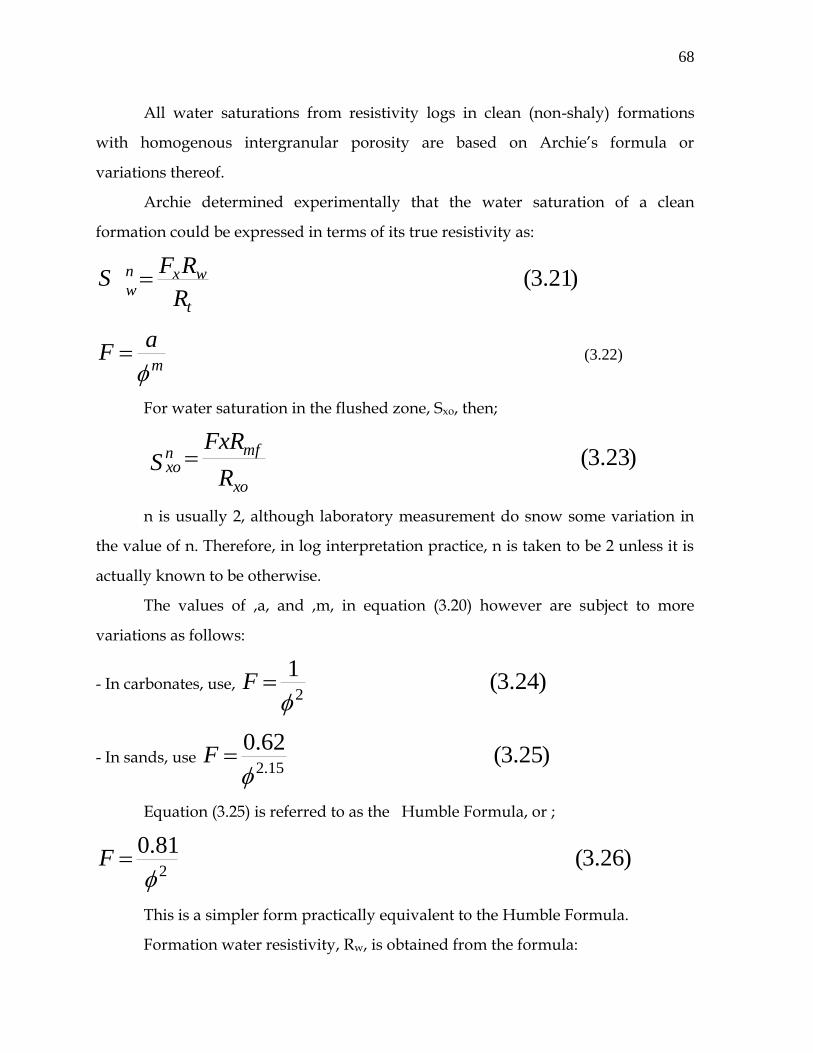
68
All water saturations from resistivity logs in clean (non-shaly) formations
with homogenous intergranular porosity are based on Archie’s formula or
variations thereof.
Archie determined experimentally that the water saturation of a clean
formation could be expressed in terms of its true resistivity as:
)21.3(t
wxn
w R
RFS
m
aF
(3.22)
For water saturation in the flushed zone, Sxo, then;
)23.3(xo
mfnxo
R
FxRS
n is usually 2, although laboratory measurement do snow some variation in
the value of n. Therefore, in log interpretation practice, n is taken to be 2 unless it is
actually known to be otherwise.
The values of ,a, and ,m, in equation (3.20) however are subject to more
variations as follows:
- In carbonates, use, )24.3(12
F
- In sands, use )25.3(62.015.2
F
Equation (3.25) is referred to as the Humble Formula, or ;
)26.3(81.02
F
This is a simpler form practically equivalent to the Humble Formula.
Formation water resistivity, Rw, is obtained from the formula:

69
wtt
wFxRR
F
RR (in shale) (3.27).
)28.3()( sandwetInRFROr wo
For clean water bearing zones, i.e. 100% water saturated formations,
wot RFRR (3.29)
And Sw = 1.
Combining equation (3.21) and (3.24) yields:
t
ww
R
RxS 2
2 1
(in carbonates) (3.30).
Combining equations (3.21) and (3.26) yields
t
ww
R
RxS 2
2 81.0
(in sands) (3.31)
As previously noted, Ro is a special case of Rt, i.e. if wet sand is being considered.
Instead of shale, Archie’s equation will be rewritten as;
02
2 81.0
R
RxS
ww
(in wet sands) (3.32).
3.9.7 THE RATIO METHOD
If n = 2 and divide equation (3.21) by (3.23), this gives;
w
mf
t
xo
xo
w
R
R
RR
SS
/2
(3.33).
This equation gives the ratio of Sw to Sxo and no knowledge of F or porosity is
needed. Rxo can be found from, say, the compensated Dual Resistivity (CDR) tool
after invasion has occurred, Rt from induction tools like CDR and the ratio Rmf/Rw
from measured values or charts.
The ratio Sw/Sxo is valuable in itself as an index of oil movability.

70
If Sw/Sxo = 1, then no hydrocarbon have been moved by invasion whether or
not the formation contains hydrocarbons. If Sw/Sxo is almost 0.5 or less, movable
hydrocarbons are indicated.
To determine Sw, from equation (3.33), Sxo must be known. For moderate
invasion and average residual oil saturation, an empirical relation between Sw and
Sxo has been found useful as follows:
Sxo = (Sw)1/5, inserting this into equation (3.33), gives;
)34.3(
85
w
mf
t
xo
wR
R
R
RS
The values of Sw/Sxo along with and Sw are useful in evaluating the
reservoir.
From this set of equations, water resistivity, Rw can be calculated using
equation (3.27) and (3.28).
Water saturation, Sw can be calculated using equations (3.30), (3.31), (3.32),
(3.43).
The true resistivity of the formation, Rt and the porosity can be calculated
or more accurately measured using a Compensated Dual Resistivity (CDR) and a
compensated Density Neutron (CDN) tool respectively.
And the hydrocarbon saturation can easily be obtained using the equation:
)35.3(1 wh SS
Any log can thus be interpreted using the obtained values of:
The water saturation, Sw
The hydrocarbon saturation, Sh,
The Resistivity Rt, Ro, Rxo or Rw
The porosity from CDN measurement and the ratio Sw/Sxo.

71
3.9.8 USING ARCHIE’S EQUATION TO DETERMINE WATER SATURATIONS
From fig 3.9 below (all the indicated values are obtained from actual log
readings), the following interpretations would be in order:
A) Zone A and C are potential Hydrocarbon bearing zones.
B) Zones B and D are water bearing zones
C) Zone B and from 7300ft downwards are hydrocarbon (oil) water contact
(OWC) zones.
Since the formation is homogenous, we can analyze the log by calculating the
formation water resistivity Rw for zone D, the water saturation, Sw, for zones A, B,
and C and hence the hydrocarbon saturation Sh for zones A, B and C as follows:

72
GR
0 API 150
RESISTIVITY
0 m 10
POROSITY
50 %
A
7350’
Rt
=4m
Sand
Shale
B
C
7400’
Rt=0.4m
Rt=8m
=0.3
=0.07
Shale
Sand
D
7500’
Ro=0.3m
=0.35
Fig. 3.9: Data from actual log readings taken in the Niger-Delta
Source: Chevron Nigeria Limited, Port Harcourt.
Note: Before using the values of resistivities indicated in the diagram to calculate for
water saturation, there is need to make use of the appropriate correction charts to
correct for borehole and shoulder bed (bed-thickness) effects.
- Calculation of formation water resistivity Rw for zone D.
Zone D is predominantly wet sand, therefore from equation (3.29),:
wo RFR

73
For sandy formations, using equation (3.26), :
2
81.0
F
Substitute F, into equation (3.28),then;
2
81.0
wo
RxR
)36.3(81.0
2
ow
xRR
From the log readings of Fig 9,
R0 = 0.3, and = 0.35
=> Rw = 045.081.0
3.035.0 2
x
0hm-m
Calculation of water saturation Sw for Zone A. Using equation (3.31) Archie’s
Equation for sandy Formations, gives;
t
w
w R
RxS 2
2 81.0
From fig. 3.9, Rt = 4 ohm-m, = 0.3 and Rw = 0.045 ohm-m as calculated for
the homogenous formation.
=> 32.04
045.0
3.0
81.02
2 ww
SxS
%32 wS
Calculation of water saturation Sw, for zone B
Again, using equation (3.31), (Archie’s equation for sandy formation), gives:
t
ww
R
RxS
2
2 81.0
From fig 3.9, Rt = 0.4 ohm-m, = 0.3 Rw = 0.045 ohm-m as calculate for the
homogenous formation.
=> %10014.0
045.0
3.0
81.02 SS ww
x

74
Calculation of water saturation Sw, for Zone C
Also, using equation (3.31), (Archie’s equation for sandy formations):
t
w
w R
RxS 2
2 81.0
Where Rt = 8ohm-m, from fig 3.9 = 0.35 and Rw = 0.045ohm-m as calculated
for the homogenous formation.
%95
96.04.0
045.0
35.0
81.02
2
SS wwx

75
3.9.10 EQUILIBRIUM INITIALIZATION ALGORITHM FOR DETERMINING
PRESSURE IN A RESERVOIR
Fig. 3.10 Depths for Initialization Algorithm
Suppose a grid block (reservoir cross section) has a gas-oil contact (GOC) and
a water-oil contact (WOC) as shown in figure 3.10 above. The pressure at GOC is
PGOC. Similarly, the pressure at WOC is PWOC. The initial oil phase pressure
assigned to the grid block is determined by PWOC, PGOC and the depth of the node
(midpoint) relative to the respective contact elevations.
The oil density ROwoc and water density RWwoc at WOC are calculated using
the pressure PWOC. The water-oil capillary pressure PCOW is calculated for the
gridblock at the midpoint elevation EL using the densities at WOC.
Considering the equation for pressure,
)47.3(hgP
From the gridblock in figure 3.10, analogously,
PCOW = )48.3(.144
1ELWOCRORW wocwoc
The initial water saturation SWI for the gridblock is calculated at the
midpoint elevation using PCOW and the following algorithm:
EL(+) (+)
(+)
y
x
Datum
WOC
GOC

76
1) IF PCOW ≥ PWOC at irreducible water saturation Swr, Set SWI = Swr
2) If PCOW ≤ PCOW at water saturation, Sw = 1, set SWI = 1.
3) If PCOW (Sw=1) < PCOW < PCOW (Sw=Swr), then interpolate the value of
SWI from the user-input water-oil capillary pressure curve.
The notation PCOW (Sw=1) should be read as the variable (PCOW) is
evaluated at Sw=1, since PCOW is a function of Sw. Similarly, the notation PCOW
(Sw=Swr) says that the variable PCOW is evaluated at Sw=Swr.
A similar calculation is performed to determine initial oil phase pressure at
the GOC using gas and oil densities. The gas density RGGOC and Oil Density ROGOC
at GOC are calculated using the pressure PGOC. The gas-oil capillary pressure
PCGO is calculated for the gridblock at the midpoint elevation EL using the
densities at GOC, thus:
PCGO = ).49.3().(144
1ELGOCRGRO GOCGOC
The initial gas saturation (SGI) and initial oil saturation (SOI) for the
gridblock are calculated at the midpoint elevation using PCGO, the previous
calculation of SWI, and the following algorithm.
a) If PCGO ≤ PCGO at total liquid saturation S1 = 1, set SGI = 0.
b) If PCGO ≥ PCGO at SL = Swr, set SGI = 1 – SWI
c) If PCGO (SL = 1) < PCGO < PCGO (SL=Swr), then, interpolate the value of SGI
from the user-input water-oil capillary pressure curve.
The notation PCGO (SL = 1) should be read as the variable PCGO is evaluated
at SL = 1 since PCGO is a function of SL. Similarly, the notation PCGO (SL = Swr) says
that the variable PCOW is evaluated at SL = Swr
Oil saturation is obtained from equation ; S0 + Sw + Sg = 1
The initial oil phase pressure is calculated using the saturations determined
above to define the appropriate pressure gradient. The algorithm for calculating P
follows:
CASE 1: IF SWI = 1, then,

77
P = PWOC +
)50.3()1(
144
1
S
RW
w
woc
PCOW
WOCEL
CASE 2: If SOI > O, then
P = PWOC - )51.3(.144
1ELWOCROwoc
CASE 3: If SGI>O and SOI = O, then
P = PWOC + WOCELROwoc 144
1
ELGOCROGOC 144
1
)52.3()1(144
1 gGOCc SPCGOGOCELRO
A natural gas-water system can be initialized by setting PWOC = PGOC and
WOC = GOC + E, where E is an incremental displacement such as 1ft.

78
3.4.1 BASIC ECONOMIC CONCEPT OF RESERVOIR MANAGEMENT
Economic analyses are an essential aspect of a reservoir management study.
The economic performance of a prospective project is often the deciding factor in
determining whether to undertake a project. Consequently, it is important to be
aware of basic economic concepts and factors that may affect the economic
performance of a project.
3.4.2 DEFINITIONS OF SELECTED ECONOMIC MEASURES
1. Discount Rate – Factor to adjust the value of money to a base year.
2. Net Present Value (NPV) – Value of cash flow at a specified discount rate.
3. Discounted Cash Flow Return On Investment (DCFROI) or Internal Rate of
Return (IRR) – Discount rate at which NPV = 0
4. Discount Payout Time – Time when NPV = 0
5. Profit-to-Investment (PI) Ratio – Undiscounted cash flow without capital
investment divided by total investment.
3.4.3 EVALUATION OF ECONOMIC MEASURES IN RELATION TO OIL
PRODUCTION
NPV is the difference between the present value of revenue R and the present
value of expenses E,
i.e.
)53.3(ERNPV
Taking Δ (K) as the expenses incurred during a time period K, then E may be written
as
NXQ
OKk
E )54.3(
Q
i1
E(K)
Also, for revenue R, ;

79
NXQ
OKk
E )55.3(
Q
i1
R(K)
where ΔR(k) is revenue obtained during time period K, and i is the annual
interest or discount rate. Equations (3.54) and (3.55) include the assumptions that i
and i' are constants over the life of the project, but i and i' are not necessarily equal.
These assumptions help to compute the present value of money expended relative to
a given inflation rate i' and compare the result to the present value of revenue
associated with a specified interest or discount rate i.
3.4.4 EVALUATION OF NPV AND BREAKEVEN OIL PRICE
The NPV and breakeven oil price for an oil production project can be
obtained from the above analysis as an illustration of the concepts. The base year
can be specified for present value calculations as the year when the project begins. In
this case, no initial revenue and the initial expense is just initial investment II, thus,
ΔR(o) = 0 and ΔE (o) = 11 (3.56)
Substitute Eq (3.53) and (3.55), into Eq (3.52) gives;
NXQ
OK
NXQ
kkk
IINPV )57.3(
Q
i'1
E(K)
Q
i1
R(K)
1
But revenue from the sale of oil during period K has the form,
ΔR(k) = Po )58.3()(Q
i1 KNP
k
Notice that the value of produced gas is assumed negligible in the case.
Combining Eq (3.56), (3.57), and (3.58) yields NPV for this project.
)59.3(
Q
i'1
)(11
Q
i1
)(Q
i'1
;11
NXQ
kk
NXQ
kk
k
okE
kNP
NPVthusP

80
where Po k
Q
i'1 ΔNP (k) = ΔR(k)
The incremental oil production in Eq. (3.59) is typically obtained as a forecast
using reservoir engineering methods like decline curve analysis, material balance
analysis, or reservoir simulation. The oil production profile used in the economic
analysis may represent both historical and predicted oil recovery.
A balance oil price Poe for a specified rate of return = ROR and production
profile is calculated by setting NPV = 0, as the breakeven conditions in Eq. (3.59).
Rearranging the resulting equation and setting Po=Poe gives the estimate of
breakeven oil price as:
)60.3(
)(1
1
1
)(11
1
'
1'
NXQ
k
pk
QROR
k
Qi
NXQ
kk
Qi
oe
kN
kE
P
3.4.5 ANALYSIS OF CAPITAL EXPENDITURE, OPERATING EXPENDITURE
AND DISCOUNT RATE
Revenue can be expressed as ;
R = )61.3()1(1
N
nn
nn
r
QPNPV
The quantity produced can be volume of oil or gas, kilowatt – hours of
electricity or any other appropriate measure of resource production.(Sharma,2003).
Expenses include capital expenditure, CAPEXn during year n, operating
expenditure, OPEXn during year n, and taxes TAXn during year n. Capital
expenditures are the cost of facilities such as offshore platforms and pipelines.
Operating expenses include on-going expenses such as salaries and maintenance
costs.
Then, the resulting expression for expenses is;
)62.3()1(1
N
nn
nnn
r
TAXOPEXCAPEXE
Substituting equations (3.60) and (3.61), into equation (3.52) gives;

81
)63.3()1(1
N
nn
nnnnn
r
TAXOPEXCAPEXQPNPV
Equation 3.62 above shows that NPV depends on the price of the resources,
the quantity of the produced resource, discount rate, capital expenditures, operating
expenditures and taxes.

82
CHAPTER FOUR
RESULTS AND ANALYSIS
The Agbara oil well reservoir investigated using the area-depth concept model was
viable. This is because, considering the related petrophysical parameters involved in
the evaluation, the reservoir was found to contain an oil deposit of 295.8 x 10⁶ stb.
Also, for the recovery factor evaluation of the reservoir, it was found the amount of
oil recovered, out of this deposit depends on the presence or absence of aquifer
influx. This was seen from the calculation of the ultimate recovery (UR) of the oil
from the reservoir. For example, the amount recovered for a case where there is a
strong aquifer influx was 153.82 x 10⁶ stb. The amount of recovery for a case where is
no aquifer influx was 136.1 x 10⁶ stb. These results showed that the reservoir
investigated was economically viable.
This method of evaluating reservoir viability is believed to be more economical
and direct in the calculation of Stock Tank Oil Initially In Place(STOIIP) and the
Ultimate Recovery Factor (URF) analysis. Although it depends on the type of the
reservoir equipment used and other uncertainties in measurements of the
petrophysical parameters.
ANALYSIS OF THE MAJOR PETROPHYSICAL PARAMETERS IN THE
RESERVOIR EVALUATION
EFFECTIVE POROSITY
This is a measure of the interconnected pore spaces as a function of bulk volume. It is the
ratio of the volume of interconnected pore space to the total volume of the rock. Effective
porosity is responsible for the migration of oil to the well bore.
b
gb
b
p
V
VV
V
VPorosity
Where Vb = Bulk volume of rock, Vp = pore Volume of rock Vg = Grain Volume of Rock.
The porosity of rock for the reservoir evaluated was 0.25. In the calculation of porosity of a
reservoir rock, sample of the core was measured to determine its length and diameter. Then,
the bulk volume, Vb, was calculated from the relation; Bulk volume,
pVVwherev
m ,1

83
Considering the mass of the oil sample and its gravity, Vp was then determined.
In another reservoir with different value of porosity, the oil deposit would be different
depending on its value. The higher the effective porosity of the rock in any reservoir, the
higher the yield and vice versa.
PERMEABILITY (K)
The absolute permeability K, of a rock is a measure of its ability to transmit a fluid when
saturated fully by the fluid as defined through Darcy’s law. It is a property of the rock and is
independent of the fluid.
The effective permeability of rock to a fluid K (Sf) is a measure of the ability of the rock to
transmit the fluid in the presence of other fluids. This depends on the saturation of the fluid
with Kf B(Sf) increasing from zero at critical saturation.
The relative permeability of a fluid krf (Sf) is the ratio of the ability of a rock to
transmit the fluid when partially saturated by the fluid to its ability to transmit the same fluid
when fully saturated by it.
Thus;
oilforK
SKSK
waterforK
SKSK
fluidanyforK
SKSK
wowro
wwwrw
ff
frf
,
,
,)(
Application of Darcy’s Law
The basic law governing fluid flow in a porous medium is Darcy’s law. The law states that
the average velocity of flow through a porous medium is proportional to the rate of pressure
change in the direction of flow l
p
d
d, and inversely proportional to the fluid viscosity, µ.
Mathematically ,L
pKAq
The negative sign is because flow is positive in the direction of reducing pressure
PA
LqK
The permeability is directly proportional to the rate of production of oil from the reservoir
rock, area of the reservoir rock and pressure change. It is also inversely proportional to the
viscosity and the rock gradient.

84
The permeability of Agbara oil well reservoir was very high. That was the reason
why there was an ultimate oil recovery of up to 153.82x10⁶
stb. The fluid flow between the
rock interconnected pores was high because of the low viscosity of the oil.
FORMATION VOLUME FACTOR
This is the volume occupied at reservoir conditions by one stock tank barrel of oil plus all the
gas originally dissolved in it. The volume of oil entering the stock tank at the surface is less
than the volume of oil which flows into the well bore from the reservoir.
This change is due to the following factors.
The most important factor is the evolution of gas from the oil as pressure is decreased
from reservoir pressure to surface conditions. This causes a large decrease in oil
volume if there is a significant amount of dissolved gas.
Other minor changes include the expansion of the remaining oil due to reduction in
pressure. But this is somewhat offset by the contraction of the oil due to the reduction
in temperature.
The evaluated Agbara Oil well has an initial formation volume factor of 1.23 rb/stb. The
lower the amount of formation volume factor, the higher the amount of stock tank oil initially
in place (STOIIP). And if the FVF is high, this will considerably lead to a lower yield of oil
in place in the reservoir. The same is applicable to another type of reservoir, regardless of the
values of other petrophysical parameters of the reservoir in question.
Net-To- Gross Ratio
In the reservoir rocks, there are some parts of sand that are not porous. These sands are
discounted with what is known as the net-to-gross ratio, F, where F is the fraction of the total
sand volume that is considered to be porous.
sandgrosstheofThickness
sandnettheofThicknessFRatioGrossToNet ,
The estimation of net-to-gross ratio on a field wide scale was accomplished by integrating
rock property trends and high quality 3-Dimensional Seismic Data. Accurate estimates of
sand volume fraction (1-Vsh) are obtainable from a simple linear interpolation between the
Acoustic Impedance (A1) – Shear Impedance (S1) trends. Four angle range stacks from a 3-
dimensional survey over the reservoir were calibrated and constrained by available well
control and simultaneously inverted to A1-S1 cross plot. The impedance volume closely
matches the upscale log data and were combined using linear interpolation between the sand

85
and shale trends to create a sand fraction volume. Integration of the sand fraction over the
gross reservoir thickness provides an estimate of Net –To – Gross ratio at any x-y Location.
Net –To – Gross evaluation is often a key issue in reservoir characterization projects.
In Agbara oil well reservoir, the Net – To – Gross Ratio, F, was found to be 0.8. This
high value of F accounted for the high yield of oil deposit in the reservoir and also
contributed to high recovery factor evaluation.
In most cases, if F is not considered and effectively measured, it normally affects the
oil yield.
HYDROCARBON POTENTIAL PAY ZONES IN A RESERVOIR USING
ARCHIES’ LAW
From the results obtained in the application of Archie’s law by combining the
related petrophysical parameters in calculating water and hydrocarbon saturations,
the different zones can be analyzed as follows;
ANALYSIS OF DIFFERENT ZONES
ANALYSIS OF ZONE A
Analysis of this zone shows that the hydrocarbon saturation of zone A is;
1-Sw = 1-0.32 = 0.68 = 68%.
This implies that zone A is hydrocarbon bearing formation. This can be
attributed to the very high porosity of 0.3 for Zone A.
ANALYSIS OF ZONE B
The calculated water saturation for Zone B is 99%, implying that it contains
100% water.
ANALYSIS OF ZONE C
The hydrocarbon saturation for zone C is 1-Sw = 1-0.96 = 0.04 = 4%. This
implies that this is not a hydrocarbon bearing formation despite the high resistivity.
This is because of the very low porosity of 0.07 for zone C.

86
EQUILIBRIUM INITIALIZATION ALGORITHM
From the algorithm developed for pressure determination in a reservoir, it was
shown that the major factors to consider in this algorithm are;
A, The initial water saturation of the reservoir(SWI).
B, The pressure at the water oil contact (PWOC).
C, The initial gas saturation of the reservoir (SGI).
D, The initial oil saturation of the reservoir (SOI).
E, The pressure at the gas-oil contact (PGOC).
F, The application of user-input water – oil capillary

87
CHAPTER FIVE
5.0 DISCUSION
In the evaluation of a reservoir, the contractor has to consider the viability of
the reservoir. This is done by estimating the quantity of stored oil in the reservoir.
That is , the calculation of the Stored Tank Oil Initially In Place (STOIIP), by taking
into account , the geometry and the related petrophysical parameters of the
reservoir. It is not feasible to extract all the oil stored in a reservoir, no matter the
sensitivity or accuracy of equipment used and the experience of the drilling
contractors. At abandonment condition, oil is still left in the well. So, before drilling
a particular well, the engineers have to justify the economic level of the reservoir.
This is achieved by estimating the recovery factor, which is the amount of hydro-
carbon that is deemed recoverable from a particular reservoir. This recovery factor
(RF) analysis helps companies to know the maximum quantity of oil that can be
drilled out from the well. It also helps to now the budget estimates to be made
before production starts. Also in a reservoir with variable quantity of hydrocarbon
at different zones, the stored oils in these zones can be calculated by the combination
of related petrophysical parameters using Archie’s law.
In this study, area-depth concept model was used to estimate the STOIIP in a
reservoir. The recovery factor of Agbara oil well was properly analyzed by this
concept. It was shown that the reservoir is economically viable. This model was
developed to analytically estimate the initial oil in place and the recovery factor in a
particular reservoir. This method of reservoir evaluation could be seen to be more
economical and direct although its efficacy depends solely on the sensitivity and
accuracy of the equipment used for the analysis of the well logs and cores. It also
depends on the experience of the drilling engineers and the reservoir conditions, if
the related petrophysical parameters are considered and measured accurately. In
this research, initialization algorithm was developed for determination of pressure
gradient in a reservoir. This pressure check helps the engineers to have an idea of
the reservoir conditions in order to prevent lost circulation and kick effects, during
drilling.

88
On the economic analysis of a reservoir, if the production quantity N, is
known, the expenses to be incurred are the capital expenditure which are the cost
facilities such as off sure platforms and pipeline arrangement. Also, the operating
expenses like the salaries of workers and maintenance costs are to be analyzed.
5.1 EXPLORATION ECONOMICS
For the optimization of drilling operations, there is need to specify the yardstick by
which performance is measured. The most relevant yardstick is cost per meter or foot drilled.
Overall cost must be looked at since individual costs can be misleading. To optimize drilling
economics, the objectives of the well must be achieved as economically as possible. In order
to do this, the cost allocations and proportions in drilling operations must be understood. The
need is to reduce the expenditure without affecting safety or efficiency.
COST SPECIFICATIONS
Exploration cost can be broken down into three groups:
1. Fixed cost
2. Daily cost
3. Unit cost
Fixed costs: These are the costs that are determined mainly by the nature of the well and
include the following:
i. Wellheads
ii. Site preparation
iii. Casing
iv. Cementing
v. Tubing
vi. Packers

89
Daily cost: Daily costs are related to the time spent on the operation. On offshore rigs, they
are usually the largest items of expenses and are listed below:
i. Payments to drilling contractors
ii. Tool rental (iii) Payments to specialist services
iv. Lubricating wages etc. (v) Fuel
vi. Drilling consumables (rope, soap and dope)
vii. Transport of materials
Unit Costs: This is the price of a unit or a commodity such as the price per tonne of barryte
or benetonite. This can be optimized in the tending process and good site supervision can
ensure that consumption is not excessive.
5.2 SPECIFIC COST BREAKDOWN OF AN OFFSHORE EXPLORATION
WELL
This is a breakdown of costs associated with a typical exploration well. The total time
spent on the well is 60 days.
FIXED COSTS
Fixed item Cost in Naira (N) (Thousands) % of Well Cost
Location survey 1600 6.20
Rig Mob/demob 2700 10.40
Casing 5700 21.90
Wellheads 1800 6.90
Drill bits 1400 5.40
Cementing 1700 6.50
Electric Logging 3200 12.30
Coring 600 2.30
Testing Equipment 1000 3.80
Rig Positioning 80 0.30
Total =N20500 Total =76.00%
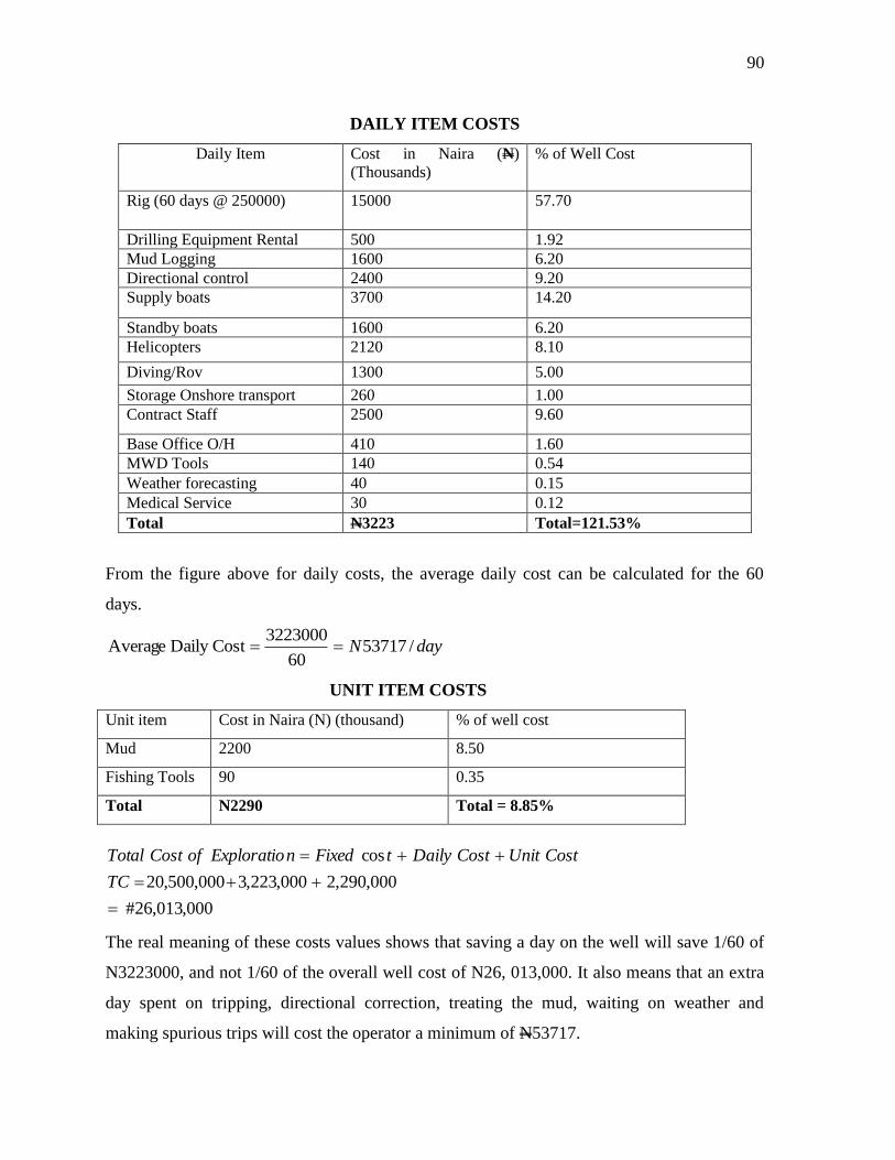
90
DAILY ITEM COSTS
Daily Item
Cost in Naira (N)
(Thousands)
% of Well Cost
Rig (60 days @ 250000) 15000 57.70
Drilling Equipment Rental 500 1.92
Mud Logging 1600 6.20
Directional control 2400 9.20
Supply boats 3700 14.20
Standby boats 1600 6.20
Helicopters 2120 8.10
Diving/Rov 1300 5.00
Storage Onshore transport 260 1.00
Contract Staff 2500 9.60
Base Office O/H 410 1.60
MWD Tools 140 0.54
Weather forecasting 40 0.15
Medical Service 30 0.12
Total N3223 Total=121.53%
From the figure above for daily costs, the average daily cost can be calculated for the 60
days.
dayN /5371760
3223000CostDaily Average
UNIT ITEM COSTS
Unit item Cost in Naira (N) (thousand) % of well cost
Mud 2200 8.50
Fishing Tools 90 0.35
Total N2290 Total = 8.85%
000,013,26#
000,290,2000,223,3000,500,20
cos
TC
CostUnitCostDailytFixednExploratioofCostTotal
The real meaning of these costs values shows that saving a day on the well will save 1/60 of
N3223000, and not 1/60 of the overall well cost of N26, 013,000. It also means that an extra
day spent on tripping, directional correction, treating the mud, waiting on weather and
making spurious trips will cost the operator a minimum of N53717.
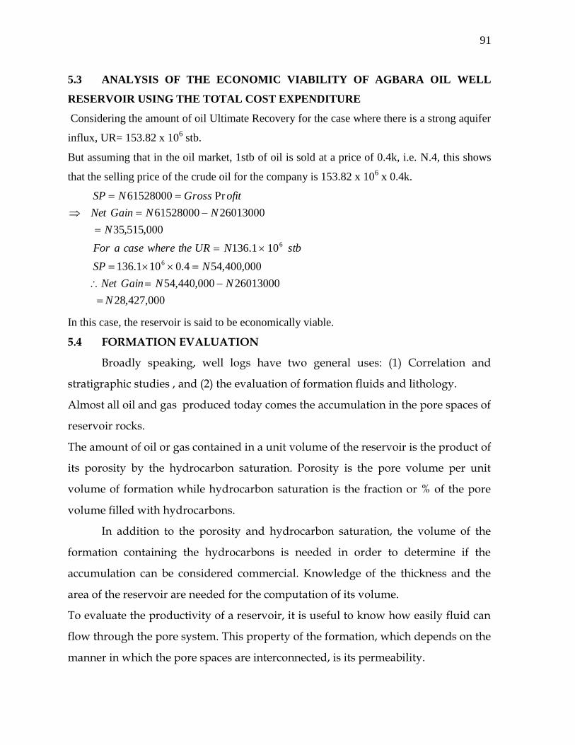
91
5.3 ANALYSIS OF THE ECONOMIC VIABILITY OF AGBARA OIL WELL
RESERVOIR USING THE TOTAL COST EXPENDITURE
Considering the amount of oil Ultimate Recovery for the case where there is a strong aquifer
influx, UR= 153.82 x 10⁶ stb.
But assuming that in the oil market, 1stb of oil is sold at a price of 0.4k, i.e. N.4, this shows
that the selling price of the crude oil for the company is 153.82 x 106 x 0.4k.
000,427,28
26013000000,440,54
000,400,544.0101.136
101.136
000,515,35
2601300061528000
Pr61528000
6
6
N
NNGainNet
NSP
stbNURthewherecaseaFor
N
NNGainNet
ofitGrossNSP
In this case, the reservoir is said to be economically viable.
5.4 FORMATION EVALUATION
Broadly speaking, well logs have two general uses: (1) Correlation and
stratigraphic studies , and (2) the evaluation of formation fluids and lithology.
Almost all oil and gas produced today comes the accumulation in the pore spaces of
reservoir rocks.
The amount of oil or gas contained in a unit volume of the reservoir is the product of
its porosity by the hydrocarbon saturation. Porosity is the pore volume per unit
volume of formation while hydrocarbon saturation is the fraction or % of the pore
volume filled with hydrocarbons.
In addition to the porosity and hydrocarbon saturation, the volume of the
formation containing the hydrocarbons is needed in order to determine if the
accumulation can be considered commercial. Knowledge of the thickness and the
area of the reservoir are needed for the computation of its volume.
To evaluate the productivity of a reservoir, it is useful to know how easily fluid can
flow through the pore system. This property of the formation, which depends on the
manner in which the pore spaces are interconnected, is its permeability.

92
This project has shown mainly the determination of water saturation using fix
values of porosity. It also explains how logs are used to obtain valuable information
about permeability, lithology, and producibility and to distinguish between oil and
gas.
Among the major parameters obtained directly from logs, resistivity is of
particular importance. It is essential to saturation determinations. Resistivity
measurements are used singly and in combination, to deduce formation resistivity
in the uninvaded formations. That is, beyond the zone contaminated by borehole
fluids, and also close to the borehole, where mud filtrate has largely replaced the
original fluids. Resistivity measurements, along with porosity and water resistivity ,
are to obtain values of water saturations. Saturation values from both shallow and
deep resistivity measurements are to evaluate the producibility of a formation.
5.5 WELL TEST ANALYSIS
Well test analysis as the name implies is the analysis of reservoir pressure
response.
These pressure responses are obtained from Pressure Recorders.
In the past, pressure recorders are lowered to the bottom of the well with the
aid of Amerada within the lubricator. Recently the practice is to place electronic
recorders permanently to retrieve information on the reservoir pressure and
temperature response.
STANDARD TESTS
The main purpose of test design is to plan a dynamic measurement sequence
and to select hardware to ensure that data acquired at the well site satisfies the test
objective and is cost efficient.
Some common well test types are; closed-chamber test,
Constant-pressure flow,
Formation-test, horizontal well test, impulse test, multilayer transient test,
multiwell interference test, pumped-well test, stabilized-flow test, step-rate test,
resistivity formation test etc.

93
5.6 IMPORTANCE OF WELL TEST ANALYSIS
Conducting well test enables us to;
Obtain reservoir fluid (oil, gas and water) samples for analysis.
Measure the maximum flow rate deliverable from the formation.
Determine reservoir and well conditions representative of the production
performance.
Analysis of the well test data enables the determination of
Average reservoir pressure
Well bore static and flowing gradients
Permeability (K)
Reservoir extent (boundary) and architecture
Skin factor (damage or stimulation)
Average pressure I’
Productivity indices.

94
5.7 COMMON TYPES OF RESERVOIR
There are three main types of reservoirs which includes
Oil reservoir
Gas reservoir
Geothermal reservoir (steam, super heated aquifer)
Test carried out on oil reservoir is called OIL WELL TEST, and test carried out on
gas reservoir is called GAS WELL TEST.
Common types of test
The choice of test type depends on test objective but the common test types includes;
a) Drawdown test (FG/DD/SG)
b) Buildup test (FG/BU/SG)
c) Drill stem test
d) Interference test
e) Back pressure test (Gas well)
FG flowing gradient, DD drawdown
SG static gradient,
BU builds up.
WELL TEST ANALYSIS HELP TO EVALUATE;
Production potential
Well damage
Average reservoir pressure
Formation characteristic
Collection of fluid samples
BASIC DATA REQUIREMENT
Rate, pressure and tune
Core/log data
RFT plots
Structural map
Well completion diagram

95
Near by test results
5.8 APPLICATION OF FLUID PRESSURE TO DETERMINE GOC, GWC, OWC.
(a). Contact (Hydrocarbon Column) Determination
Where the fluid contacts (OWC, GWC, GOC) are not obtainable directly from
well log either due to tool failure, poor hole conditions (washouts) shaly formations
or the structural location of the well then well pressure can be measured to
determine them.
The first step is to establish an appropriate water line by measuring water
pressures in the vicinity of the hydrocarbon region. Then:
(1). To determine Oil-Water Contact (OWC) or Gas-Water Contact (GWC) in any
sand-Measure pressure from at least 3 depths in the hydrocarbons in that
send to establish the oil or gas line as the case may be. The intersection of the
oil line with the water the given the position of the OWC while the
intersection of the gas line with the water line gas the GWC. Remember that if
only gas and water have been seen then there is the possibility for an oil film
in between. Smaller the effect of errors due to tool positioning and accuracy.
So choose depths as far apart as possible within the zone under evaluation.
Attempt to take pressures especially for contact determination in one run. Re-
runs/calibrations/depth correlations could make some difference.
Give regard to hole conditions-washouts. Tight formations, etc while
selecting depths for pressure measurement. Also avoid depths too close to
contacts and formation boundaries.
All depths must be converted to a common vertical reference depth. Usually
TVDs which is the vertical depth below the mean sea level. Place more
confidence in points requiring less deviation corrections due to possible
errors in calculating these corrections as well as errors in the deviation data
themselves.
While hydrostatics implies straight line relation of pressure with depth.
Graphical solutions are preferred to algebraic solutions as there are many

96
subtle revelations that usually only appear on plots. Be careful not to regress
out useful trends! Be contions about joining pressure points across barriers.
Always be guided by typical gradients. Do not just get the best line through
the points (the best line may be the wrong line). There may be more straight
line and totally different interpretation.
Be aware that as in all extrapolations, the farther away from the region of
measured data you are the less the confidence in the results. Remember spill
points and other structural limits.
Make sure the water line is applicable to the hydrocarbon region you are
evaluation (SITP,2000).
5.9 PRESSURE AND TEMPERATURE GAUGE PLACEMENT
The following procedure are observed for down-hole gauge or recorder
placement;
1) Fro offshore well tests two sets of electronic recorder called upper and lower
gauges are run below the Tester Valve. These gauges are usually placed 4ft or
6ft apart as the case may be. Generally for onshore, one recorder is enough.
2) In both onshore and offshore at least one recorder should be run above, the
chokes or above the tester valve if no chokes are available.
3) All the electronic recorders is use mush have mechanical pressure recorders
as a back-up. A minimum of one mechanical temperature recorder should
also be used for back-up.
4) At least one pressure recorder should be ported so as record annular
pressure.
5) One recorder set consisting of electronic pressure/temperature recorder
should be run as close to the perforation as possible (Bottom gauge).
6) One recorder set consisting of electronic pressure/temperature recorder and
mechanical pressure recorder should be run approximately midway between
the tester value and perforation, if this distance is significant (top gauge).
7) Pressure and temperature elements should be selected such that formation
pressure and temperatures fall within the application range to enable

97
recorder survive bull-heading pressure if required. In absence of better data,
bull-heading pressure may be assumed to be 1.0 to 1.2 psi per foot of depth.
8) Recorder operating times (mechanical check and operating frequencies)
should be selected, to allows for the total running-in time plus the total of all
the anticipated flow and shut-in times. Running-in time should be based on
similar tests offsetting walls. When data are unavailable running-in time can
be approximated as 1 hour per 1000 it of depth per 4 hours for final rig-up.
9) Time delays of pressure switch start should not be relied on for all electronic
recorders.
10) Pressure STOPS should be made near the vicinity of gas lift Mandrels, close to
the top and bottom of sand to capture contacts and around the perforation
intervals. Stop duration should be at least 15 minutes for all electronic
recorders.
5.9.1 GAUGE PERFORMANCE CHECK
Once the recorders have been retrieved a qualitative analysis of the pressure
charts is performed to verify that the test was successful. This is otherwise referred
to as Quality Check.
Points to be examined includes the following;
a) Did the recorder work?
b) Were all the flow and build-up period recorded?
c) Are the top and bottom recorder charts similar appearance?
d) Is the final hydrostatic pressure similar to the initial hydrostatic pressure?
e) Do the recorded pressures correlated to what actually occurred.
f) Are the charts and data analyzable?
GAUGE PERFORMANCE CHECK PROCEDURE
1) Load the pressure test data from the diskette (ASCII FILE) for the top and
bottom gauges.
2) From the menu command, zip on difference and activate the difference plot.
3) For the table of data locate
i) Flow period

98
ii) Early build-up
iii) Late build-up
iv) Static period
4) With the zoom facility pick ranges on each of the selected flow periods and
examine the responses of both gauges.
5) Repeat the process for temperature gauges.
5.9.2 PRESSURE PROGRAMMING AND INTERPRETATION FOR RFT ANALYSIS
Fluid pressures are measured using the open hole RFT tool run wire line
usually after the resistivity and porosity logs. To a limited extent, cased hole
RFT is carried out where sever hole problems prevent open hole RFT logging.
The tool is normally fitted with both a strain gauge and quartz crystal gauge.
Always use the quartz gauge for interpretation. The strain gauge (less
susceptible to failure but less accurate) should be a health check that all is
well with the quartz gauge. Ensure that all gauges are properly calibrated
before use.
State clearly the objectives of the pressure programme and make sure how all
the pressure points relate to these objectives. Try to see how points could
fulfill multiple objectives to minimize the total number of points. RFT is very
expensive because apart from the logging costs. The pressure readings are
taken while the tools is not only stationary but properly pressed (could say
clamped) to the formation. This greatly increases the chance of getting the
tool stuck after making a pressure reading. The last thing you want to
imagine is getting stuck and possibly loosing the entire well that has been
drilled at considerable cost while making a pressure measurement that could
have been avoided.
Establish a water line in the vicinity of the hydrocarbon bearing sands at any
opportunity of running the tool regardless of the specific objectives of the
particular well. This could be used in interpreting pressures in other well in

99
the field where water intervals are not encountered. It may indeed save the
drilling of an appraisal well.
Two points always form a straight line so you need at last a third point to
confirm the existence of the line.
5.9.3 LABORATORY ANALYSIS OF OIL SAMPLES
Data usually obtained from laboratory analysis include;
1) Original reservoir temperature of person
2) Pressure volume relation at one or more temperature are of which is always
the reservoir temperatures
3) Variation of surface separator pressure with and amounts of gas liberated as
shrinkage of oil resulting from separator process.
4) Differential gas liberation and oil shrinkage data
5) Density and specific volume of reservoir fluid.
6) Variation of oil viscosity with pressure at reservoir pressure to atmospheric
pressure also viscosity of stock tank oil.
100
CHAPTER SIX
6.0 CONCLUSION
Almost all oil and gas produced today comes from accumulation in the pore spaces of
reservoir rocks. The amount of oil or gas contained in a unit volume of the reservoir is the
product of its porosity and the hydrocarbon saturation. In addition to the porosity and
hydrocarbon saturation, the volume of the formation containing the hydrocarbons is needed
in order to determine if the accumulation can be considered commercial.
In this study, the initial oil and gas volumes was calculated from depth contour maps
(horizon maps), reservoir rocks and fluid properties of the Agbara oil well reservoir, which
was used as a case study. The results obtained from the analysis of the area – depth graph and
cumulative bulk volume graph, shows that the fluid saturations in the reservoir structure was
clearly estimated. Also, the recovery factor estimates was done. These estimates are obtained
by making certain assumptions regarding displacement efficiency, residual saturations,
abandonment columns and drive mechanisms based on experience in an operating area.
Usually, these are by correlations based on reservoir and crude properties. Sweep efficiencies
depend on oil and reservoir properties obtained from correlations based on local experience
and simulation studies. Residual saturations depend on rock type obtained from measured
averages from different rock types. Abandonment column height depend on reservoir/ oil
characteristics and well type.
To evaluate the viability of a reservoir, it is useful to know how easily fluid can flow
through the pore system. This property of the formation, which depends on the manner in
which the pore spaces are interconnected, is its permeability. This project has shown the
determination of initial oil reserve in a reservoir and the recovery factor estimates, using fix
values of related petrophysical parameters. It also explains how logs are used to obtain
valuable information about permeability, lithology and connate water saturations, and to
distinguish between oil and gas.
Resistivity measurements, along with porosity and water resistivity, are used to obtain
values of water saturation. Saturation values from both shallow and deep resistivity
measurements were compared to evaluate the viability of an oil reservoir formation.
The results obtained from the evaluation of Agbara oil well showed that the reservoir is
economically viable.

101
6.1 RECOMMENDATIONS
From the findings of this research, I wish to recommend as follows:
(A) There is need to carry out intensive research on reservoir evaluations in order to explore
and evaluate the economic and technological improvements and advantages of alternative
energy sources like oil shales and the biomass-fuel plants over fossil fuels.
(B) I also recommend that more drilling related areas be covered in the future with a more
comprehensive view on oil management.
(C) In reservoir evaluations, I recommend that there is need to improve on the quality of the
scientific log reading tools as the reservoir data needed for evaluation depend on the accuracy
and precision of this equipment.
REFERENCES
Allan J. and Q. Sun (2003): Controls on Recovery factor in Fractured
Reservoirs. SPE Annual Technical Conference.
Archie, E.G. (1982):The Electrical Resistivity Log. As an aid in
Determining some Reservoir Characteristics. Pet Tech, vol.5.
Arps, J.J. (1945): Analysis of Define Curves. Transaction of AIME, Volume
160
Craft, B.C. M.F. Hawkins and R.E. Terry (1991): Applied petroleum
Reservoir Engineering. Second Edition, Englewood Cliffs, New
Jersey Prentice Hall.
Firoozabadi, A (1996), :Recovery Mechanism In Fractured Reservoir And Field
Performance. Journal of Candian petroleum Engineers Formation
Evaluation.
Frank Shray (1997): Logging While Drilling Interpretation. The Four
Dimensions; Seminar Manual, Nigeria.

102
Green, D. W. and G.P. Whihite (1998): Enhanced Oil Recovery Richardson.
Texas Society of Petroleum Engineers.
Halderson. H.H. and Damsleth E. (1993): Challenges in Reservoir
Characterization. American Association of Petroleum Geologist Bulletin,
Volume 77, No. 4.
Lecture Note from Shell Intensive Training Program, SITP, (2000), In Nigeria.
Roman Talamantez (1996): Log Interpretation Principles and Applications.
Seminar Manual. USA.
Ron Baker (1996): A Primal of Oil Well Drilling. 5th Edition, Petroleum
Extention Services, Austin Texas, in Cooperation with international
association of drilling contractors, Houstin, texas.
Schlumberger Wire Line and testing (1993): People and Technology. A
directional Drilling Training manual by Schlumberger, Houston.
Schlumberger Wire Line and testing (1997): Well Evaluation Conference in
Nigeria.
Schlumberger Wire Line and testing (2000): Well Evaluation Conference in
Nigeria.
Sharma P.C. (2003): “A Textbook of Production Engineering. S.Chand and
Company LTD, 7361, New Delhi.
Sylvain Pirson J. (1958): Elements of Oil Reservoir Engineering (2nd
Ed). Ed.
New York: McGraw Hill
Texier, M.P. and Alger R. P (1965): Combine Logs Pinpoint Reservoir and
Resistivity. Biggs, R. P. Carpenter, B.N. PET TECH.
The Times: Weekened Money by Stella Shemon (1998): http//www. the times.
Co.uk/news.
Timmerman E.H. Mcmahon J.J. and Everdinen A.F. (1953): Application of the
Material Balance Equation to a partial water- Drive Reservoir. Trans.
AIME.

103
SAMPLE
QUESTIONNAIRE
AND
APPENDIX

104
APPENDIX A
QUESTIONARE
SAMPLE OF QUESTIONNAIRE
Dear Respondent,
My name is Ngwu Japhet Ifeanyi. I am a postgraduate student of University
of Nigeria, Nsukka Department of Mechanical Engineering. I am carrying out a
project work on reservoir evaluation.
The questions below are intended to provide information about the use of
petrophysical parameters in the evaluation of a crude oil reservoir.
Please, fill the boxes or fill in relevant information in the gap provided. Also
where necessary, kindly provide data in the spaces provided. Your kind co-
operation in sincerely answering the questions will provide a basis for the use of
petrophysical parameters in the evaluation of a crude oil reservoir
A: GENERAL INFORMATION
1. Respondent’s position in the company:
2. Name and address of your company:
3. Number of years you have worked in the company
4. Year the company is established 19
5. Types of ownership:
Sole proprietorship
Partnership
Public limited company
Public liability company
Joint venture
6. Describe your company ownership structure;
1) Wholly indigenous

105
2) Wholly expatriate
3) Indigenous %
4) and expatriate %
7. Indicate the engineering services offered by your company:
Engineering design/consultancy
Engineering construction/installation
Maintenance and calibration company
Engineering services, design, installation and maintenance
Exploration and mining company
Oil servicing company
Others (specify):
B: QUESTIONS ON RESERVOIR EVALUATION
8. What is an oil reservoir?
9. What is the mechanism behind the production of oil in a reservoir?
10. What are the main petrophysical parameters needed for reservoir
evaluations?
11. Does this company have standard established methods for determination of
STOIIP? Yes: No:
12. If yes, which type of method does the company normally use and why the
method?
13. Are there established methods of analyzing petrophysical logs from a
particular reservoir by your company? Yes: No:
14. If yes, name the petrophysical parameter and the method of analysis
________________________________________________
15. Does your company have electronic log tools for petrophysical analysis or
do they hire external contractors? ? Yes: No:
16. If yes, what are the name of the tools and how are they used specifically?

106
17. During the estimation of oil reserve in a reservoir, does it purely depend
on the precision and accuracy of the equipment used?
Yes: No:
18. What are the terms GOC and OWC and how are they determined in a
particular reservoir?
19. How is planimeter used in the determination of area at a particular reservoir?
20. What is a net-to-gross sand ratio and how is it determined in a particular
reservoir?
21. Does connate water saturation have a standard value or does it differ
according to the nature of a reservoir?
22. Please Sir, what is RFT analysis?
23. Why is the net-go-gross ratio F, important in oil estimation in a reservoir?
24. How is the net-go-gross sand ratio, F, porosity Ø, and connate water
saturations Swc determined in a particular reservoir?
25. What are the necessary petrophysical parameters needed for recovery
factor evaluations?
26. What happens at the Gas zone, Oil zone and Water zone in the
abandonment conditions?
27. Is there any laboratory test analysis of an oil sample from a particular
reservoir before drilling?
28. What is well test analysis?
29. What are the different test analysis conducted on well and type of
equipment used?
30. Do you people apply the volumetric method of estimation in
determination of STOIIP? Yes: No:
31. If no, does it mean that volumetric method is insufficient?

107
32. What need to be added in this method for it to be applicable in reservoir
evaluation?
33. How is the pressure gradient determined in a reservoir and the need for pressure
analysis before drilling? ________________________________________________
34. How can Archie’s law be applied in the analysis of hydrocarbon zones in a
particular reservoir? ____________________________________
35 What are the basic economic factors to consider during exploration from a
particular reservoir? ___________________________________________________

108
APPENDIX B
CONVERSION
43560FT2 = 1 ACRE – Ft
43560Ft3 = 1 acre ft = 1
1 acre ft 43560Ft3
Vo = Ah ø S0 acre – ft x 43560ft3
1 acre – ft
:. V0 = 43560 Ah ø S0 – Ft3
But 5.615ft3 = 1bbl
V0 = 43560 Ah ø S0 – ft3 x 1bbL
5.615ft3
:. Vo = 7758 Ah ø S0- rb .
From Equation (1.6), we have
Sw + S0 + Sg = 1,
where Sg 0 (vaporizes)
:. Sw + S0 = 1
S0 = 1- Sw
Therefore, V0 = 7758Ah ø (1-Sw) stb
β0
Where Vo = Volume of Oil
A = Area of the reservoir
h = Height of the reservoir
ø = Porosity of the reservoir
β0 = Formation volume factor
Unit stb = stock Tank Barrel
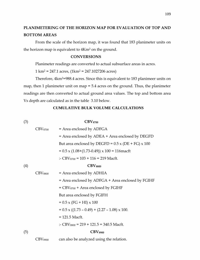
109
PLANIMETERING OF THE HORIZON MAP FOR EVALUATION OF TOP AND
BOTTOM AREAS
From the scale of the horizon map, it was found that 183 planimeter units on
the horizon map is equivalent to 4Km2 on the ground.
CONVERSIONS
Planimeter readings are converted to actual subsurface areas in acres.
1 km2 = 247.1 acres, (1km2 = 247.1027206 acres)
Therefore, 4km2=988.4 acres. Since this is equivalent to 183 planimeer units on
map, then 1 planimeter unit on map = 5.4 acres on the ground. Thus, the planimeter
readings are then converted to actual ground area values. The top and bottom area
Vs depth are calculated as in the table 3.10 below.
CUMULATIVE BULK VOLUME CALCULATIONS
(3) CBV8700
CBV8700 = Area enclosed by ADFGA
= Area enclosed by ADEA + Area enclosed by DEGFD
But area enclosed by DEGFD = 0.5 x (DE + FG) x 100
= 0.5 x (1.08+(1.73-0.49)) x 100 = 116macft
:- CBV8700 = 103 + 116 = 219 Macft.
(4) CBV8800
CBV8800 = Area enclosed by ADHIA
= Area enclosed by ADFGA + Area enclosed by FGIHF
= CBV8700 + Area enclosed by FGIHF
But area enclosed by FGIFH
= 0.5 x (FG + HI) x 100
= 0.5 x ((1.73 – 0.49) + (2.27 – 1.08) x 100.
= 121.5 Macft.
:- CBV8800 = 219 + 121.5 = 340.5 Macft.
(5) CBV8900
CBV8900 can also be analyzed using the relation.

110
Bulk volume = (sum of the difference in TOP & Base) x (8900-8800)
2
= (2.81 – 1.73) + (2.27-1.08) x (8900 x 8800)
2
= 113.5 Macft
:- CBV8900 = BV8900 + CBV8800
= 113.5 + 340.5 = 454.00Macft.
(6) CBV9000
CBV9000 is analyzed as:
Bulk volume = (3.24-2.27) + (2.81-1.73) x (9000-8900)
2
= 102.5macft
:- CBV9000 = BV9000 + CBV8900
= 102.50 + 454.00 = 556.50 Macft
OIL ULTIMATE RECOVERY FOR CASE WHERE THERE IS NO AQUIFER
INFLUX
A case where there is no aquifer and BVw=0.00, Boa = 1.17 rb/stb
Since BVw = O, Final OWC = Original OWC = 8800ft, Boa=1.23 rb/stb
Final GOC = final OWC – Ha = 8800-40 = 8760ft
But BVa = CBVowc – CBVaoc
BVa = CBV8800 – CBV8760 = 340.5 – 291.5 = 49Macft (from graph)
BVg = CBV8760 – CBV8560 = 291.5 – 64.3 = 227.3 Mac-ft.
But BV = BVa + BVg + BVw = 49 + 227.3 + O = 276.3 Mac-ft.
Applying the recovery factor equation (3.26)
RF = 1 – Boi {BVg[Eg Sorg + (1-Eg)(1-Swc-Sg)] + BVw [Ew Sorw+(1-Ew)(1-Swc-Sg)]+BVa(1-Swc-Sg)}
BoaBV(1-Swc)
:- RF = 1 – 1.23 {227.3[0.7 x 0.15 + (1-0.7) x (1-0.15-0.02)]+49 x (1-0.15-0.02)] = 0.46
1.17 x 276.3 x 0.85
=> Oil Ultimate Recovery = STOIIP x RF
= 295.8 x 106 x 0.46 = 136.1 x 10⁶ Mstb.

111

112
APPENDIX C
PLANNING OF RESERVOIR SIMULATION
PROBLEM DEFINITION
Clear statement of objectives and scope of the simulation study.
Well studies – coning/well testing
Cross section (2D) studies – cupping, vertical heterogeneity, pseudo, landing
depths/completing intervals.
Element studies – vertical /horizontal well completion, well interference,
fault scal, arcal sweep
Full field studies – HCIIP, key appraisal parameters, development options,
reservoir management.
DATA GATHERING
Structural – formation tops, fault sealing potentials
Maps/geological model.
Reservoir description – Rock types/distribution correlations, baffle extent –
logs, cores and deposition model.
Rock properties per type -, Kn, Ky- Logs/cores/ wells tests /RFT- MDT
(Resistively formation Test multiple Dimensional Test) – Kr, S0r Pc, Cf- special
core analysis
Fluid properties – PVT studies
Fluid contacts – Logs,RFT
Aquifer Data – material balance.
MODEL CONSTRUCTION
GIRDING – grid block size just enough to capture variation 1-20k
Averaging /assignment of rock properties
Input of fluid properties
Initialization Data- original fluid contacts
Aquifer data input
Well data input – location, kn, skw, lift and constraints, production data.

113
MODEL VALIDATION
Limitalization – check values of STOIIP, FGIIP and contacts
History matching in honesty + common sense
- matching parameters
- Pressure profile ( time/arcal)
- Well GOR
- Fluid contacts
- Rates
- Matching variables ( what to adjust within honest realistic ranges,
discuss with geologist).
K, Kv/Kh values and profiles
Relative permeabilities – Block/ well
Fault seals
Aquifer parameters
FORECASTING
Reward of development activities/decisions
off take level
Well type, number and location
fluid injection type, location and volumes
Surface facility constraints
Tiring of activities – infill, recompletion, artificial lift, injection, etc.
REPORTING
Objectives
Model description
Model validity – quality of match /sensitivity, further data requirement and
assumptions.
Results of scenario studies
Optimum development option and forecast

114
PRODUCTION FORECATING
True production forecast should be from one or more of the techniques considered
so far:
Material balance analysis
Analytical recovery calculations
Numerical reservoir simulation studies.