Evaluation of various Algorithms to detect acoustic Feedback · PDF fileS. Braun: Feedback Detection 3 ... frequencies between about 200 and 5000 Hz . The howling has a very narrow-band

Evaluation of various Algorithmsto detect acoustic Feedback

Toningenieur Projekt

Sebastian Braun

Betreuung: DI Hannes Pomberger

Graz, February 19, 2012

institut für elektronische musik und akustik

Abstract

Annoying howling caused by acoustic feedback is an omnipresent problem inamplified live-sound situations. There are some algorithms that detect feedbackhowling frequencies automatically and try to eliminate these via notch filters. Forthe detection of the feedback frequencies, several different approaches and criteriaare available, that can be used separately or in combination. The proposed algo-rithms shall be implemented and evaluated in a suitable simulation environment.In this work, a new evaluation method is designed, that is more objective than theproposed evaluation in literature. Two evaluation methods are introduced, but thefinal evaluation focuses on the new developed method.Further, the improvement of the detection algorithms by using a Constant-Q-Analysis, and the additional use of a second microphone are investigated. Thissecond microphone can gather additional information, such as the estimation ofmaximum stable gain (MSG) of the amplification system and might improve theperformance.The evaluation results of several detection criteria form a basis for an advanceddesign of a feedback detector.

S. Braun: Feedback Detection 3

Contents

1 Introduction 5

1.1 How occurs feedback howling? . . . . . . . . . . . . . . . . . . . . . . . 5

1.2 Notch filter based howling suppression . . . . . . . . . . . . . . . . . . 6

2 Available Criteria 7

2.1 Single-feature criteria . . . . . . . . . . . . . . . . . . . . . . . . . . . 7

2.2 Multi-feature criteria . . . . . . . . . . . . . . . . . . . . . . . . . . . . 9

3 Implementation and optimization 9

3.1 Peak picking algorithm . . . . . . . . . . . . . . . . . . . . . . . . . . . 10

3.2 Improvement of the PHPR algorithm . . . . . . . . . . . . . . . . . . . 10

3.3 Cascade temporal criterion IPMP with other criteria as post-processor . . 11

3.4 Constant-Q Analysis . . . . . . . . . . . . . . . . . . . . . . . . . . . . 12

3.5 Two Microphone Method . . . . . . . . . . . . . . . . . . . . . . . . . 12

4 Evaluation of the criteria 14

4.1 First Environment . . . . . . . . . . . . . . . . . . . . . . . . . . . . . 14

4.1.1 Evaluation method . . . . . . . . . . . . . . . . . . . . . . . . . 14

4.1.2 Defining the true howling frequencies . . . . . . . . . . . . . . . 15

4.1.3 Problems of this simulation method . . . . . . . . . . . . . . . . 16

4.2 New Simulation Environment . . . . . . . . . . . . . . . . . . . . . . . 16

4.2.1 Additional criterion: HBPF . . . . . . . . . . . . . . . . . . . . 18

5 Simulation results 18

5.1 First simulation method . . . . . . . . . . . . . . . . . . . . . . . . . . 18

5.1.1 Temporal development of Hitrate and False Alarm Rate . . . . . 19

5.2 Comparison of CQT vs. DFT . . . . . . . . . . . . . . . . . . . . . . . 20

5.3 New Real-time simulation method . . . . . . . . . . . . . . . . . . . . . 22


5.3.1 Evaluation of single criteria . . . . . . . . . . . . . . . . . . . . 22

5.3.2 Evaluation of additional post-processing criteria IPMP and HBPF 24

5.3.3 Comparison and evaluation of the best performing features . . . . 25

5.4 Subjective evaluation with PD patch . . . . . . . . . . . . . . . . . . . 28

6 Conclusion and outlook 29


1 Introduction

Almost everyone who visits pop/rock-concerts from time to time, has experienced asituation where the public adress (PA) system started to howl due to acoustic feedback.Whereas at live-music events a qualified sound engingeer is usually present at any time,especially in speech reinforcement situations a technical supervisor is not present oravailable. But even a properly equalized PA system does not guarantee a howling-freesystem. If the microphone positions are not static, i.e. a microphone is moved over thestage, the transfer functions change and new situations can occur, that weren’t takeninto account and cause unstable feedback. To handle this problem, an adaptive feedbackcanceller is a good solution. The focus of this work lies on the detection of feedbackhowling frequencies, not on cancelling or suppression methods.

1.1 How occurs feedback howling?

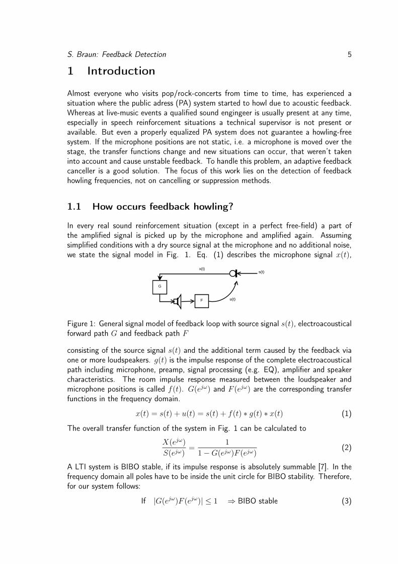
In every real sound reinforcement situation (except in a perfect free-field) a part ofthe amplified signal is picked up by the microphone and amplified again. Assumingsimplified conditions with a dry source signal at the microphone and no additional noise,we state the signal model in Fig. 1. Eq. (1) describes the microphone signal x(t),

s(t)x(t)

F

G

u(t)

Figure 1: General signal model of feedback loop with source signal s(t), electroacousticalforward path G and feedback path F

consisting of the source signal s(t) and the additional term caused by the feedback viaone or more loudspeakers. g(t) is the impulse response of the complete electroacousticalpath including microphone, preamp, signal processing (e.g. EQ), amplifier and speakercharacteristics. The room impulse response measured between the loudspeaker andmicrophone positions is called f(t). G(ejω) and F (ejω) are the corresponding transferfunctions in the frequency domain.

x(t) = s(t) + u(t) = s(t) + f(t) ∗ g(t) ∗ x(t) (1)

The overall transfer function of the system in Fig. 1 can be calculated to

X(ejω)

S(ejω)=

1

1−G(ejω)F (ejω)(2)

A LTI system is BIBO stable, if its impulse response is absolutely summable [7]. In thefrequency domain all poles have to be inside the unit circle for BIBO stability. Therefore,for our system follows:

If |G(ejω)F (ejω)| ≤ 1 ⇒ BIBO stable (3)


This means that for certain poles in the transfer function Eq. (2), our system getsunstable, even if a bounded (stable) input signal is given. Depending on the unstablefrequency pole, we perceive this unstability as howling, since it occurs most frequent atfrequencies between about 200 and 5000 Hz . The howling has a very narrow-band likecharacter similar to a single sine component, because usually only one single frequencyis unstable.

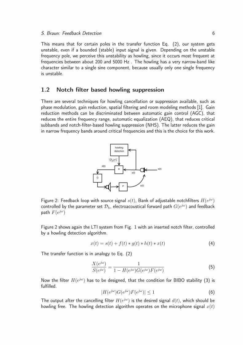
1.2 Notch filter based howling suppression

There are several techniques for howling cancellation or suppression available, such asphase modulation, gain reduction, spatial filtering and room modeling methods [1]. Gainreduction methods can be discriminated between automatic gain control (AGC), thatreduces the entire frequency range, automatic equalization (AEQ), that reduces criticalsubbands and notch-filter-based howling suppression (NHS). The latter reduces the gainin narrow frequency bands around critical frequencies and this is the choice for this work.

s(t)H

howlingdetection

x(t)

F

G

d(t)

u(t)

Figure 2: Feedback loop with source signal s(t), Bank of adjustable notchfilters H(ejω)controlled by the parameter set Dh, electroacoustical forward path G(ejω) and feedbackpath F (ejω)

Figure 2 shows again the LTI system from Fig. 1 with an inserted notch filter, controlledby a howling detection algorithm.

x(t) = s(t) + f(t) ∗ g(t) ∗ h(t) ∗ x(t) (4)

The transfer function is in analogy to Eq. (2)

X(ejω)

S(ejω)=

1

1−H(ejω)G(ejω)F (ejω)(5)

Now the filter H(ejω) has to be designed, that the condition for BIBO stability (3) isfulfilled.

|H(ejω)G(ejω)F (ejω)| ≤ 1 (6)

The output after the cancelling filter H(ejω) is the desired signal d(t), which should behowling free. The howling detection algorithm operates on the microphone signal x(t)


and outputs a set of howling frequencies for each time frame. These detected frequenciesform together with other filter design parameters the parameter set Dh(t). A notch filterdesign needs at least the center frequency, the gain reduction value and a bandwidth.An advanced notch-filter design can include a time-variant design for all parameters, notonly the center frequency. In simpler implementations some of the parameters can keptstatic, e.g. the notch-filter bandwidth.

2 Available Criteria

The paper of Toon van Waterschoot and Marc Moonen [2] is used as a starting pointfor this work. It provides a collection of various criteria for feedback howling detection.In this section, the criteria and the evaluation method proposed in [2] are explained.

The idea behind the criteria is the following: The microphone signal x(t) is bufferedand framed with a buffer size of N and hop-size R, windowed and transformed into thefrequency domain via FFT.

x(t) = [x(t+R−N) ... x(t+R− 1)]T (7)

X(ωk, t) =N−1∑n=0

w(tn)x(tn)e−jωktn (8)

As not stated different, the values N = 4096, R = 12N and a Blackman window for w(t)

are used at a sampling frequency fs = 44100 Hz. The spectra X(ωk, t) are processed bya peak picking algorithm, that delivers the angular frequencies ωi of the detected peaksas a set of “howling candidates” Dω(t). The feedback detection algorithms operateon this set of M howling candidates and calculate a certain criterion value for everyhowling candidate ωi ∈ Dω(t). If this value exceeds a threshold, the null hypothesis -H0: howling does not occur - is rejected, otherwise no howling is detected.

The simplest criterion is to take a fixed power threshold value, e.g. P0 = 85 dB SPL todecide whether a frequency bin contains feedback or not. Waterschoot collected 6 suchcriteria and one, that merges two of these into a new criterion.

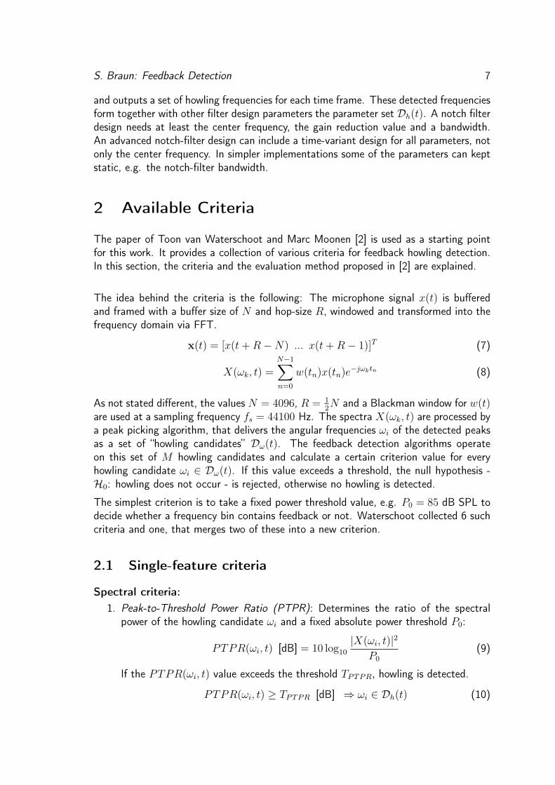
2.1 Single-feature criteria

Spectral criteria:1. Peak-to-Threshold Power Ratio (PTPR): Determines the ratio of the spectral

power of the howling candidate ωi and a fixed absolute power threshold P0:

PTPR(ωi, t) [dB] = 10 log10|X(ωi, t)|2

P0

(9)

If the PTPR(ωi, t) value exceeds the threshold TPTPR, howling is detected.

PTPR(ωi, t) ≥ TPTPR [dB] ⇒ ωi ∈ Dh(t) (10)


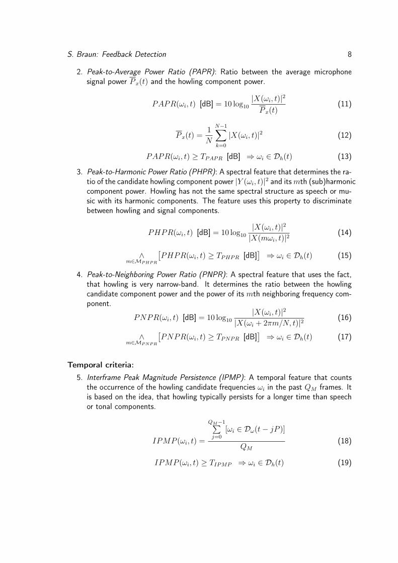
2. Peak-to-Average Power Ratio (PAPR): Ratio between the average microphonesignal power P x(t) and the howling component power.

PAPR(ωi, t) [dB] = 10 log10|X(ωi, t)|2

P x(t)(11)

P x(t) =1

N

N−1∑k=0

|X(ωi, t)|2 (12)

PAPR(ωi, t) ≥ TPAPR [dB] ⇒ ωi ∈ Dh(t) (13)

3. Peak-to-Harmonic Power Ratio (PHPR): A spectral feature that determines the ra-tio of the candidate howling component power |Y (ωi, t)|2 and its mth (sub)harmoniccomponent power. Howling has not the same spectral structure as speech or mu-sic with its harmonic components. The feature uses this property to discriminatebetween howling and signal components.

PHPR(ωi, t) [dB] = 10 log10|X(ωi, t)|2

|X(mωi, t)|2(14)

∧m∈MPHPR

[PHPR(ωi, t) ≥ TPHPR [dB]

]⇒ ωi ∈ Dh(t) (15)

4. Peak-to-Neighboring Power Ratio (PNPR): A spectral feature that uses the fact,that howling is very narrow-band. It determines the ratio between the howlingcandidate component power and the power of its mth neighboring frequency com-ponent.

PNPR(ωi, t) [dB] = 10 log10|X(ωi, t)|2

|X(ωi + 2πm/N, t)|2(16)

∧m∈MPNPR

[PNPR(ωi, t) ≥ TPNPR [dB]

]⇒ ωi ∈ Dh(t) (17)

Temporal criteria:

5. Interframe Peak Magnitude Persistence (IPMP): A temporal feature that countsthe occurrence of the howling candidate frequencies ωi in the past QM frames. Itis based on the idea, that howling typically persists for a longer time than speechor tonal components.

IPMP (ωi, t) =

QM−1∑j=0

[ωi ∈ Dω(t− jP )]

QM

(18)

IPMP (ωi, t) ≥ TIPMP ⇒ ωi ∈ Dh(t) (19)


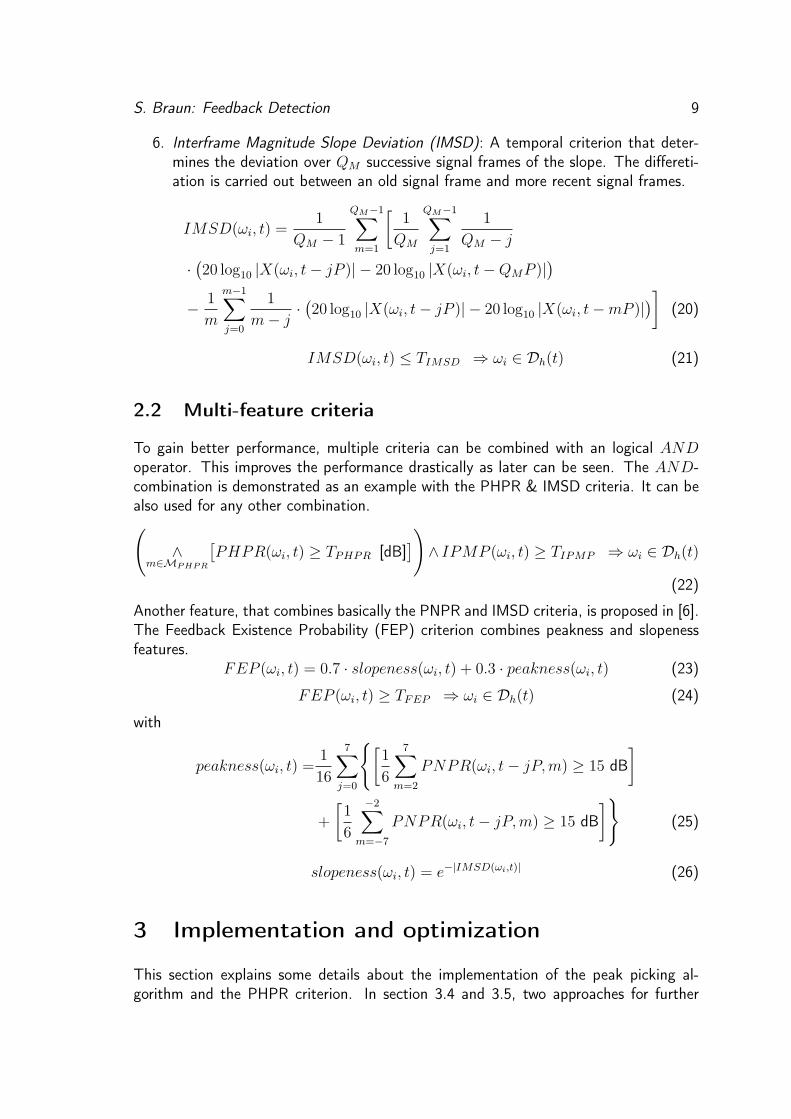
6. Interframe Magnitude Slope Deviation (IMSD): A temporal criterion that deter-mines the deviation over QM successive signal frames of the slope. The differeti-ation is carried out between an old signal frame and more recent signal frames.

IMSD(ωi, t) =1

QM − 1

QM−1∑m=1

[1

QM

QM−1∑j=1

1

QM − j

·(20 log10 |X(ωi, t− jP )| − 20 log10 |X(ωi, t−QMP )|

)− 1

m

m−1∑j=0

1

m− j·(20 log10 |X(ωi, t− jP )| − 20 log10 |X(ωi, t−mP )|

)](20)

IMSD(ωi, t) ≤ TIMSD ⇒ ωi ∈ Dh(t) (21)

2.2 Multi-feature criteria

To gain better performance, multiple criteria can be combined with an logical ANDoperator. This improves the performance drastically as later can be seen. The AND-combination is demonstrated as an example with the PHPR & IMSD criteria. It can bealso used for any other combination.(

∧m∈MPHPR

[PHPR(ωi, t) ≥ TPHPR [dB]

])∧ IPMP (ωi, t) ≥ TIPMP ⇒ ωi ∈ Dh(t)

(22)

Another feature, that combines basically the PNPR and IMSD criteria, is proposed in [6].The Feedback Existence Probability (FEP) criterion combines peakness and slopenessfeatures.

FEP (ωi, t) = 0.7 · slopeness(ωi, t) + 0.3 · peakness(ωi, t) (23)

FEP (ωi, t) ≥ TFEP ⇒ ωi ∈ Dh(t) (24)

with

peakness(ωi, t) =1

16

7∑j=0

{[1

6

7∑m=2

PNPR(ωi, t− jP,m) ≥ 15 dB]

+

[1

6

−2∑m=−7

PNPR(ωi, t− jP,m) ≥ 15 dB]}

(25)

slopeness(ωi, t) = e−|IMSD(ωi,t)| (26)

3 Implementation and optimization

This section explains some details about the implementation of the peak picking al-gorithm and the PHPR criterion. In section 3.4 and 3.5, two approaches for further


perfomance improvement are introduced. 3.5 is not included in the evaluation process,because we could not find a way, that the approach contributes to a performance im-provement. But it gives the possibility to estimate the maximum stable gain of a system.

3.1 Peak picking algorithm

The peak picking algorithm 1 - here shown for the spectral magnitude A(k) = |X(ωk)|with k = 0...N

2- searches for changes in the its deviation A′(k) from positive to negative

values. These are local maxima of A(k),

A′(k) = A(k)− A(k + 1); (27){A′(k) ≥ 0 ∧ A′(k + 1) ≤ 0} ⇒ ωk ∈ Dω

This algorithm delivers the set of peaks Dω(t). After that we drop peak values for k = 0,since a DC peak is not useful and also k = N

2− 7 ... N

2, because it is easier for the

implementation of some algorithms (PNPR, FEP), which operate on the picked peaks.At frequencies near 20 kHz the damping through loudspeakers and the air is usually thathigh, that acoustic feedback won’t occur there in a practical scenario.

3.2 Improvement of the PHPR algorithm

As stated in Eq. (14), there could occur two problems:– What if a peak with a continuous frequency |Y (ωi, t)| lies between two DFT bins|Y (ωk, t)| and |Y (ωk+1, t)|?

– What if the multiplication by the factors m does not correspond exactly to the har-monic component and misses it by some neighbor bins?

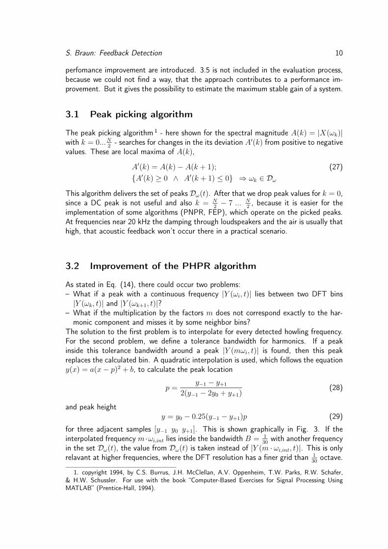
The solution to the first problem is to interpolate for every detected howling frequency.For the second problem, we define a tolerance bandwidth for harmonics. If a peakinside this tolerance bandwidth around a peak |Y (mωi, t)| is found, then this peakreplaces the calculated bin. A quadratic interpolation is used, which follows the equationy(x) = a(x− p)2 + b, to calculate the peak location

p =y−1 − y+1

2(y−1 − 2y0 + y+1)(28)

and peak heighty = y0 − 0.25(y−1 − y+1)p (29)

for three adjacent samples [y−1 y0 y+1]. This is shown graphically in Fig. 3. If theinterpolated frequency m ·ωi,int lies inside the bandwidth B = 1

30with another frequency

in the set Dω(t), the value from Dω(t) is taken instead of |Y (m · ωi,int, t)|. This is onlyrelavant at higher frequencies, where the DFT resolution has a finer grid than 1

30octave.

1. copyright 1994, by C.S. Burrus, J.H. McClellan, A.V. Oppenheim, T.W. Parks, R.W. Schafer,& H.W. Schussler. For use with the book “Computer-Based Exercises for Signal Processing UsingMATLAB” (Prentice-Hall, 1994).


0 5 10 15 20 25 300

0.5

1

1.5

signal

picked peaks

parabolic interpolated peak locations

threshold

Figure 3: Peak picking and interpolation for PHPR

3.3 Cascade temporal criterion IPMP with other criteria aspost-processor

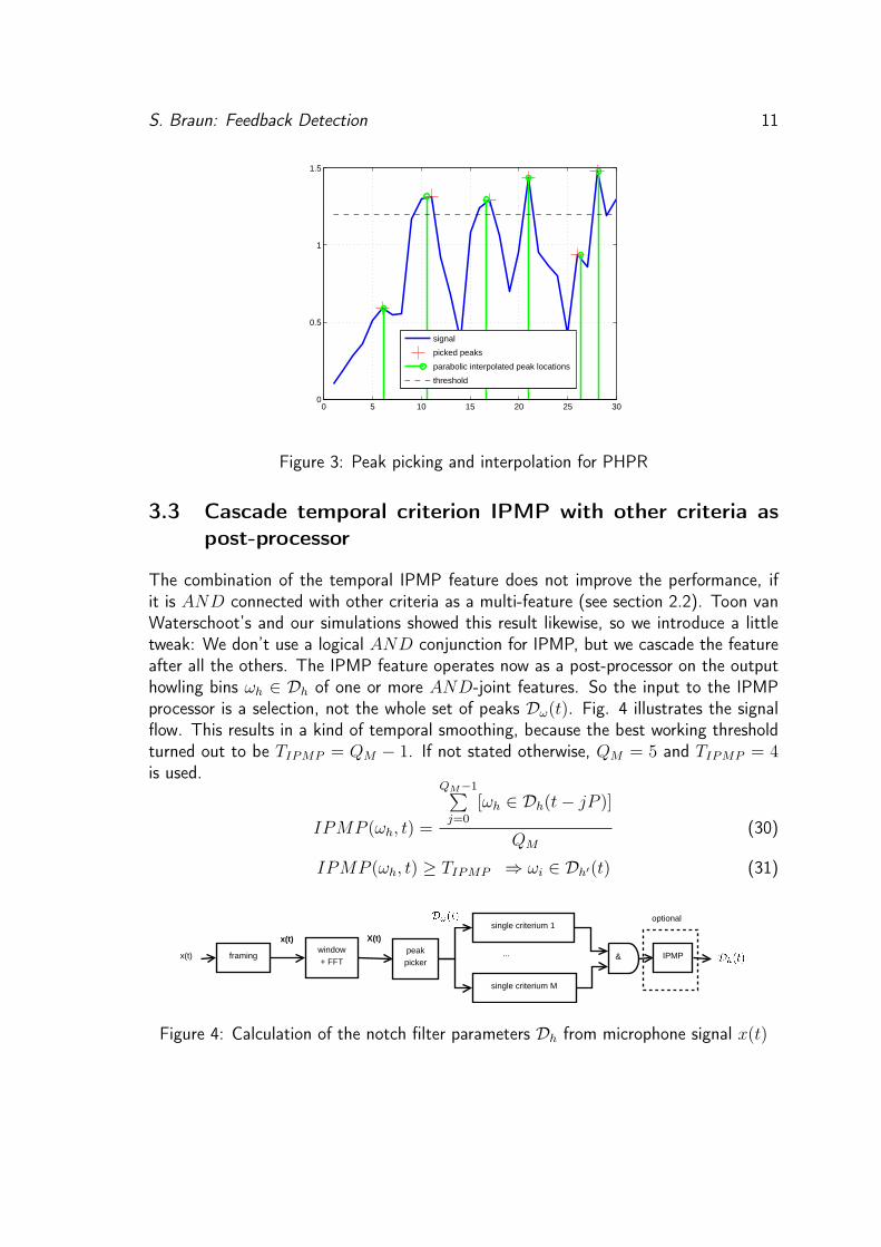
The combination of the temporal IPMP feature does not improve the performance, ifit is AND connected with other criteria as a multi-feature (see section 2.2). Toon vanWaterschoot’s and our simulations showed this result likewise, so we introduce a littletweak: We don’t use a logical AND conjunction for IPMP, but we cascade the featureafter all the others. The IPMP feature operates now as a post-processor on the outputhowling bins ωh ∈ Dh of one or more AND-joint features. So the input to the IPMPprocessor is a selection, not the whole set of peaks Dω(t). Fig. 4 illustrates the signalflow. This results in a kind of temporal smoothing, because the best working thresholdturned out to be TIPMP = QM − 1. If not stated otherwise, QM = 5 and TIPMP = 4is used.

IPMP (ωh, t) =

QM−1∑j=0

[ωh ∈ Dh(t− jP )]

QM

(30)

IPMP (ωh, t) ≥ TIPMP ⇒ ωi ∈ Dh′(t) (31)

framing

x(t) X(t)

single criterium 1

single criterium M

... & IPMPx(t)window+ FFT

peakpicker

optional

Figure 4: Calculation of the notch filter parameters Dh from microphone signal x(t)


3.4 Constant-Q Analysis

The spectral criteria PHRP and PNPR show a strongly varying performance The givenlinear frequency resolution of the DFT is quite low at lower octaves and high at theupper octaves, A logarithmic frequency resolution would fit a perceptive grid for musicalcontent as howling components better. The Constant-Q-Transformation (CQT) [3] isa suited time-to-frequency domain transformation for this problem. It allows a spectralanalysis holding logarithmic spaced spectral bins with equal bandwidth.The CQT of a discrete-time signal x(n) is defined by

XCQ(k, n) =

n+bNk/2c∑j=n−bNk/2c

x(j)a∗k(j − n+Nk/2) (32)

where the basis functions ak(n), also called time-frequency atoms are

ak(n) =1

Nk

w

(n

Nk

)exp

[−i2πn

fkfs

]. (33)

w denotes a window function and the center frequencies obey

fk = f12k−1B . (34)

The frequency dependent window length Nk computes as follows, with 0 < q ≤ 1 beinga scaling factor and B the number of bins per octave.

Nk =qfs

fk(21B − 1)

(35)

For the implementation in Matlab, the CQT-Toolbox published in [5] was used, thatgives a quick usable and efficient implementation of a constant-Q transform.

3.5 Two Microphone Method

An additional idea to get better performance of howling detection algorithms is to usea second microphone capsule, coincident or spatially separated, to get more informationand calculate the features from this second microphone signal. But since the information,the second microphone picks up, is not really different to the first microphone, the featurecalculation cannot be improved further.At least we can use the second capsule to calculate the actual gain factor a, that is placedin the electroacoustical forward path G(ejω) = a ·Gn(e

jω) with max(Gn(ejω)) = 1.

y1(t) = V1s(t) + aH1y1(t); ⇒ y1(t) =V1x(t)

1− aH1

(36)

y2(t) = H2x(t) + y1(t) · aV2 = H2x(t) +V1x(t)

1− aH1

· aV2 (37)


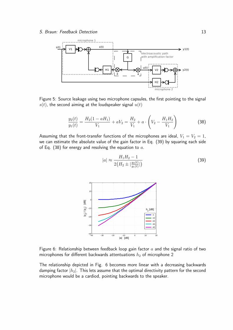
Figure 5: Source leakage using two microphone capsules, the first pointing to the signals(t), the second aiming at the loudspeaker signal u(t)

y2(t)

y1(t)=

H2(1− aH1)

V1

+ aV2 =H2

V1

+ a ·

(V2 −

H1H2

V1

)(38)

Assuming that the front-transfer functions of the microphones are ideal, V1 = V2 = 1,we can estimate the absolute value of the gain factor in Eq. (39) by squaring each sideof Eq. (38) for energy and resolving the equation to a.

|a| ≈ H1H2 − 1

2(H2 ± |y2(t)

y1(t)|) (39)

−40 −30 −20 −10 0 10 20−40

−30

−20

−10

0

10

20

|a| [dB]

|y2| /

|y1|

[dB

]

0

−10

−20

−30

−40

h2 [dB]

Figure 6: Relationship between feedback loop gain factor a and the signal ratio of twomicrophones for different backwards attentuations h2 of microphone 2

The relationship depicted in Fig. 6 becomes more linear with a decreasing backwardsdamping factor |h2|. This lets assume that the optimal directivity pattern for the secondmicrophone would be a cardiod, pointing backwards to the speaker.


4 Evaluation of the criteria

The evaluation as Toon van Waterschoot et al. did, seemed to have some weak points.After discussing the realization according to his method, another new developed methodto evaluate the algorithms is presented.

4.1 First Environment

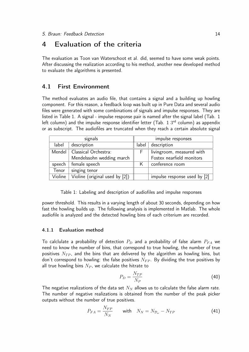
The method evaluates an audio file, that contains a signal and a building up howlingcomponent. For this reason, a feedback loop was built up in Pure Data and several audiofiles were generated with some combinations of signals and impulse responses. They arelisted in Table 1. A signal - impulse response pair is named after the signal label (Tab. 1left column) and the impulse response identifier letter (Tab. 1 3rd column) as appendixor as subscript. The audiofiles are truncated when they reach a certain absolute signal

signals impulse responseslabel description label description

Mendel Classical Orchestra:Mendelssohn wedding march

F livingroom, measured withFostex nearfield monitors

speech female speech K conference roomTenor singing tenorVioline Violine (original used by [2]) impulse response used by [2]

Table 1: Labeling and description of audiofiles and impulse responses

power threshold. This results in a varying length of about 30 seconds, depending on howfast the howling builds up. The following analysis is implemented in Matlab. The wholeaudiofile is analyzed and the detected howling bins of each criterium are recorded.

4.1.1 Evaluation method

To calclulate a probability of detection PD and a probability of false alarm PFA weneed to know the number of bins, that correspond to true howling, the number of truepositives NTP , and the bins that are delivered by the algorithm as howling bins, butdon’t correspond to howling: the false positives NFP . By dividing the true positives byall true howling bins NP , we calculate the hitrate to

PD =NTP

NP

(40)

The negative realizations of the data set NN allows us to calculate the false alarm rate.The number of negative realizations is obtained from the number of the peak pickeroutputs without the number of true positives.

PFA =NFP

NN

with NN = NDω −NTP (41)


0 0.1 0.2 0.3 0.4 0.5 0.6 0.7 0.8 0.9 10

0.1

0.2

0.3

0.4

0.5

0.6

0.7

0.8

0.9

1PNPR

PFA

PD

m ∈ {±2}

m ∈ {±2, ±3}

m ∈ {±2, ±3, ±4}

m ∈ {±1, ±2, ±3}

m ∈ {±3, ±4, ±5}

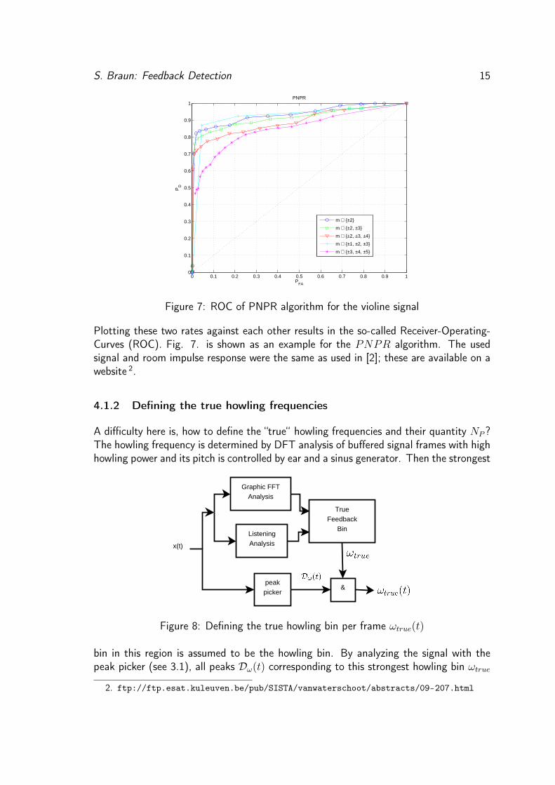
Figure 7: ROC of PNPR algorithm for the violine signal

Plotting these two rates against each other results in the so-called Receiver-Operating-Curves (ROC). Fig. 7. is shown as an example for the PNPR algorithm. The usedsignal and room impulse response were the same as used in [2]; these are available on awebsite 2.

4.1.2 Defining the true howling frequencies

A difficulty here is, how to define the “true“ howling frequencies and their quantity NP ?The howling frequency is determined by DFT analysis of buffered signal frames with highhowling power and its pitch is controlled by ear and a sinus generator. Then the strongest

peakpicker

Graphic FFTAnalysis

ListeningAnalysis

TrueFeedback

Bin

x(t)

&

Figure 8: Defining the true howling bin per frame ωtrue(t)

bin in this region is assumed to be the howling bin. By analyzing the signal with thepeak picker (see 3.1), all peaks Dω(t) corresponding to this strongest howling bin ωtrue

2. ftp://ftp.esat.kuleuven.be/pub/SISTA/vanwaterschoot/abstracts/09-207.html


are assumed to be true howling and not so the rest. This process is schematically shownin Fig. 8.

4.1.3 Problems of this simulation method

As in this method a precomputed audio file that already contains feedback is used tocalculate the feedback criteria from it, several problems arise:– With increasing file length, the howling gets more prominent.– In the sequence where the feedback level has already built up higher over the signal,

it is easy for the algorithms to detect the howling frequency.– The false alarm rate is therefore dependent on the file length, respectively on how fast

the feedback builds up and is powerful in the signal.With this method the criteria are only comparable, if one single audio file is used. Asaudio material can differ drastically, the method is not objective for all sound sources,only for the one specific tested case. For that reason another test scenario is developedas follows.

4.2 New Simulation Environment

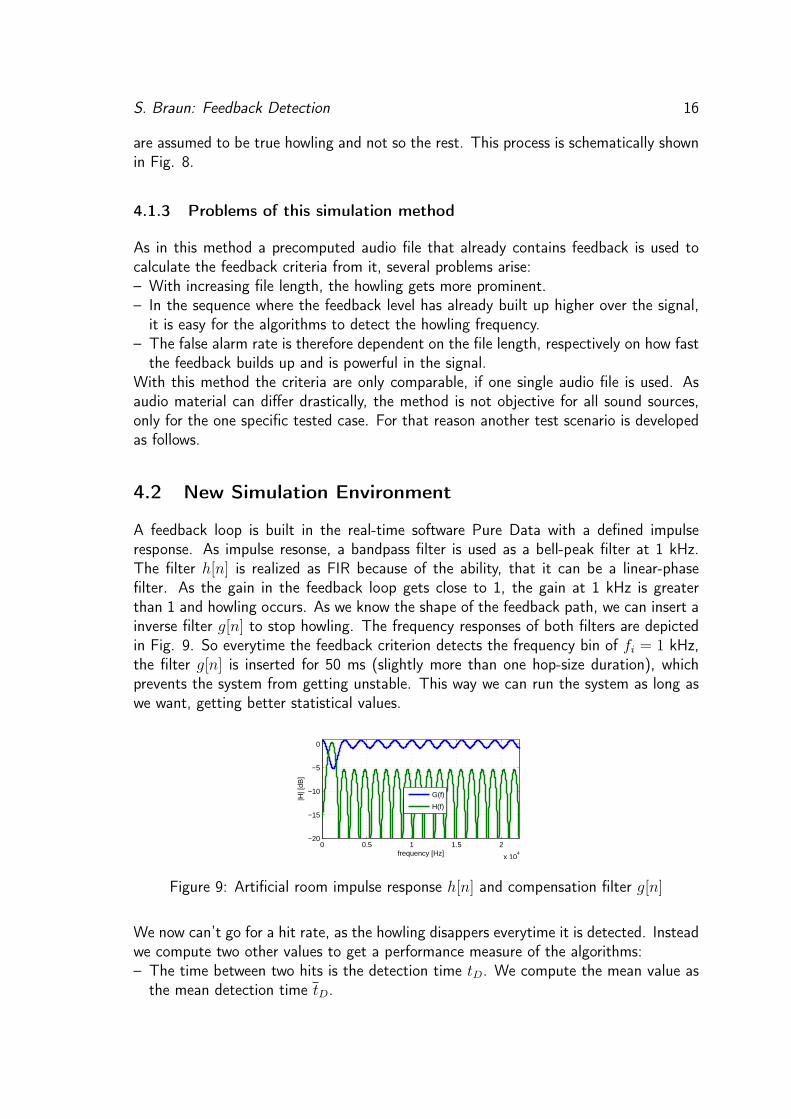
A feedback loop is built in the real-time software Pure Data with a defined impulseresponse. As impulse resonse, a bandpass filter is used as a bell-peak filter at 1 kHz.The filter h[n] is realized as FIR because of the ability, that it can be a linear-phasefilter. As the gain in the feedback loop gets close to 1, the gain at 1 kHz is greaterthan 1 and howling occurs. As we know the shape of the feedback path, we can insert ainverse filter g[n] to stop howling. The frequency responses of both filters are depictedin Fig. 9. So everytime the feedback criterion detects the frequency bin of fi = 1 kHz,the filter g[n] is inserted for 50 ms (slightly more than one hop-size duration), whichprevents the system from getting unstable. This way we can run the system as long aswe want, getting better statistical values.

0 0.5 1 1.5 2

x 104

−20

−15

−10

−5

0

frequency [Hz]

|H| [

dB]

G(f)

H(f)

Figure 9: Artificial room impulse response h[n] and compensation filter g[n]

We now can’t go for a hit rate, as the howling disappers everytime it is detected. Insteadwe compute two other values to get a performance measure of the algorithms:– The time between two hits is the detection time tD. We compute the mean value as

the mean detection time tD.


– The signal power of the whole feedback loop. The longer the algorithm needs todetect and cancel the right howling frequency, the higher the signal power rises.

The signal can influence the mean detection time tD since it can take longer for howlingto build up, if the signal power is very weak or zero right after the filter g[n] is deactivated.The other way round, tD can be very short if the signal power is great. So if we takethe average signal power, we have a quite good measure for how much howling occursin the system, until it gets detected and cancelled.

To get a relative value, a second reference feedback loop is built with the filters h[n] andg[n] always activated. We now measure the signal power of the actual feedback loopES(t) and the reference system Eref (t) and can get a relative power value in Eq. (42)by dividing the mean values. E describes how much additional signal power is added byhowling because of the system being unstable.

E =ES(t)

Eref (t)(42)

The system is depicted in Fig. 10 with the actual feedback loop on top and the referenceloop below. Since the filter g[n] introduces a delay of d samples to the forward path, adelay expressed as Dirac-Delta function δ[n] compensates the path without g[n]. Theonly purpose of the reference loop is to calculate Eref . The gain factor a controls theamount of feedback. If |ah[n]| > 1 for one frequency bin (1 kHz in this case), the systemgets unstable and starts howling at this frequency.

Figure 10: Feedback loop and reference loop. The detection algorithm switches the filterg[n] in for 50 ms to keep the loop stable.


Testsignals To reduce the effort of the simulation, three test signals are chosen. Theyhave already been presented in section 4.1. We chose only single instrument sources,since in a given situation it is more likely that we have a close-miking setup. The threetest samples are the Violine, a singing Tenor and female Speech, that are labeled likely.

4.2.1 Additional criterion: HBPF

A new criterion is introduced because of the signal-interactive behaviour of this newdeveloped evaluation method. In contrast to the method proposed in 4.1, it mattershere especially in terms of the detection speed, that can’t be measured with the methodof section 4.1.The detected howling frequencies Dh(t) are straight used to steer the set of notch-filters.A further idea, how to lower the detection of false howling frequencies, is based on thisassumption: Only one frequency per time frame can be a true howling feedback, allothers are assumed to be false detected ones. To prevent this, only the Highest Bin PerFrame (HBPF) from the set Dh(t) is taken, that means the howling component withthe greatest power. Using this additional criterion, only one notchfilter can be changedor set per frame.

HBPF (ωh, t) = max(|X(ωh, t)|

)(43)

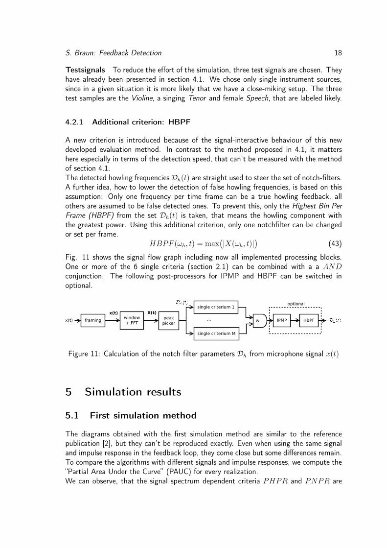
Fig. 11 shows the signal flow graph including now all implemented processing blocks.One or more of the 6 single criteria (section 2.1) can be combined with a a ANDconjunction. The following post-processors for IPMP and HBPF can be switched inoptional.

Figure 11: Calculation of the notch filter parameters Dh from microphone signal x(t)

5 Simulation results

5.1 First simulation method

The diagrams obtained with the first simulation method are similar to the referencepublication [2], but they can’t be reproduced exactly. Even when using the same signaland impulse response in the feedback loop, they come close but some differences remain.To compare the algorithms with different signals and impulse responses, we compute the“Partial Area Under the Curve” (PAUC) for every realization.We can observe, that the signal spectrum dependent criteria PHPR and PNPR are


influenced by some characteristics of the signals or impulse responses, for example ifthe howling frequency bin is shared with a harmonic part of the signal, or the howlingfrequency lies exactly between two bins. For the other features, the tendencies remainmore constant in relative manner. The simplest features PTPR and PAPR seem tobe the best though.

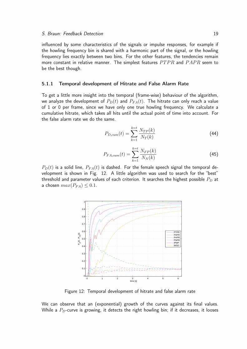
5.1.1 Temporal development of Hitrate and False Alarm Rate

To get a little more insight into the temporal (frame-wise) behaviour of the algorithm,we analyze the development of PD(t) and PFA(t). The hitrate can only reach a valueof 1 or 0 per frame, since we have only one true howling frequency. We calculate acumulative hitrate, which takes all hits until the actual point of time into account. Forthe false alarm rate we do the same.

PD,cum(t) =k=t∑k=1

NTP (k)

NT (k)(44)

PFA,cum(t) =k=t∑k=1

NFP (k)

NN(k)(45)

PD(t) is a solid line, PFA(t) is dashed. For the female speech signal the temporal de-velopment is shown in Fig. 12. A little algorithm was used to search for the “best”threshold and parameter values of each criterion. It searches the highest possible PD ata chosen max(PFA) ≤ 0.1.

0 1 2 3 4 5 60

0.1

0.2

0.3

0.4

0.5

0.6

0.7

0.8

0.9

1

time [s]

PD

(t)

, PF

A(t

)

PTPRPAPRPHPRPNPRIPMPIMSD

Figure 12: Temporal development of hitrate and false alarm rate

We can observe that an (exponential) growth of the curves against its final values.While a PD-curve is growing, it detects the right howling bin; if it decreases, it looses


the howling. IPMP has the smallest problem with losing the howling, because it is justkind of a temporal smoothing filter. Fig. 12 also points out very good that the resultsof the ROC-Curves differ, depending on the audiofile length. One can read the temporalprobability values by just cutting vertically through the curves at one specific point oftime.The PAPR algorithm has found the true howling frequency from the beginning. But theproblem of this evaluation method is clarified most with the PAPR-curve: The longerthe audio segment is, the more PFA grows against zero. So this evaluation methoddiminishes the evaluation emphasis of the critical phase, where the howling begins tobuild up and is not louder than the signal. But this is the critical and essential phase ofsuch an algorithm. If the howling power lies already several dB over the signal power,it is easy to detect the howling. The early phase where howling builds up, is where thealgorithms should later operate at, because if they detect howling, it will be immediatelynotched out. That’s the reason why the second evaluation method in 4.2 is developed.

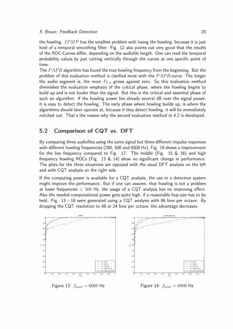
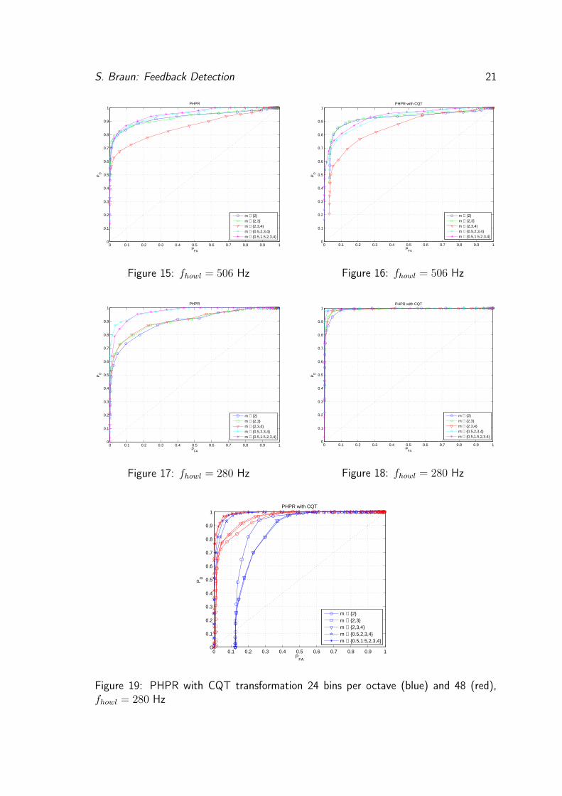
5.2 Comparison of CQT vs. DFT

By comparing three audiofiles using the same signal but three different impulse responseswith different howling frequencies (280, 506 and 6008 Hz), Fig. 18 shows a improvementfor the low frequency compared to Fig. 17. The middle (Fig. 15 & 16) and highfrequency howling ROCs (Fig. 13 & 14) show no significant change in performance.The plots for the three situations are opposed with the usual DFT analysis on the leftand with CQT analysis on the right side.

If the computing power is available for a CQT analysis, the use in a detection systemmight improve the performance. But if one can assume, that howling is not a problemat lower frequencies < 500 Hz, the usage of a CQT analysis has no improving effect.Also the needed computational power gets quite high, if a reasonable hop-size has to beheld. Fig. 13 - 18 were generated using a CQT analysis with 96 bins per octave. Bydropping the CQT resolution to 48 or 24 bins per octave, the advantage decreases.

0 0.1 0.2 0.3 0.4 0.5 0.6 0.7 0.8 0.9 10

0.1

0.2

0.3

0.4

0.5

0.6

0.7

0.8

0.9

1PHPR

PFA

PD

m ∈ {2}m ∈ {2,3}m ∈ {2,3,4}m ∈ {0.5,2,3,4}m ∈ {0.5,1.5,2,3,4}

Figure 13: fhowl = 6008 Hz

0 0.1 0.2 0.3 0.4 0.5 0.6 0.7 0.8 0.9 10

0.1

0.2

0.3

0.4

0.5

0.6

0.7

0.8

0.9

1PHPR with CQT

PFA

PD

m ∈ {2}m ∈ {2,3}m ∈ {2,3,4}m ∈ {0.5,2,3,4}m ∈ {0.5,1.5,2,3,4}



0 0.1 0.2 0.3 0.4 0.5 0.6 0.7 0.8 0.9 10

0.1

0.2

0.3

0.4

0.5

0.6

0.7

0.8

0.9

1PHPR

PFA

PD

m ∈ {2}m ∈ {2,3}m ∈ {2,3,4}m ∈ {0.5,2,3,4}m ∈ {0.5,1.5,2,3,4}


0 0.1 0.2 0.3 0.4 0.5 0.6 0.7 0.8 0.9 10

0.1

0.2

0.3

0.4

0.5

0.6

0.7

0.8

0.9

1PHPR with CQT

PFA

PD

m ∈ {2}m ∈ {2,3}m ∈ {2,3,4}m ∈ {0.5,2,3,4}m ∈ {0.5,1.5,2,3,4}


0 0.1 0.2 0.3 0.4 0.5 0.6 0.7 0.8 0.9 10

0.1

0.2

0.3

0.4

0.5

0.6

0.7

0.8

0.9

1PHPR

PFA

PD

m ∈ {2}m ∈ {2,3}m ∈ {2,3,4}m ∈ {0.5,2,3,4}m ∈ {0.5,1.5,2,3,4}


0 0.1 0.2 0.3 0.4 0.5 0.6 0.7 0.8 0.9 10

0.1

0.2

0.3

0.4

0.5

0.6

0.7

0.8

0.9

1PHPR with CQT

PFA

PD

m ∈ {2}m ∈ {2,3}m ∈ {2,3,4}m ∈ {0.5,2,3,4}m ∈ {0.5,1.5,2,3,4}


0 0.1 0.2 0.3 0.4 0.5 0.6 0.7 0.8 0.9 10

0.1

0.2

0.3

0.4

0.5

0.6

0.7

0.8

0.9

1PHPR with CQT

PFA

PD

m ∈ {2}m ∈ {2,3}m ∈ {2,3,4}m ∈ {0.5,2,3,4}m ∈ {0.5,1.5,2,3,4}

Figure 19: PHPR with CQT transformation 24 bins per octave (blue) and 48 (red),fhowl = 280 Hz


Fig. 19 shows the low-frequency howling file with 24 (blue) and 48 (red) bins/octave.With 48 bins/octave there is still a small improvement to Fig. 17, using just 24 binsmight be a quality decrease. Another advantage of a CQT analysis is the variable windowlength, decreasing with the frequency. This might be useful for a howling detection aswell, since lower frequencies build up slower than high frequencies. This corresponds tothe low hop-size of the CQT at the bottom and a high hop-size on the top.

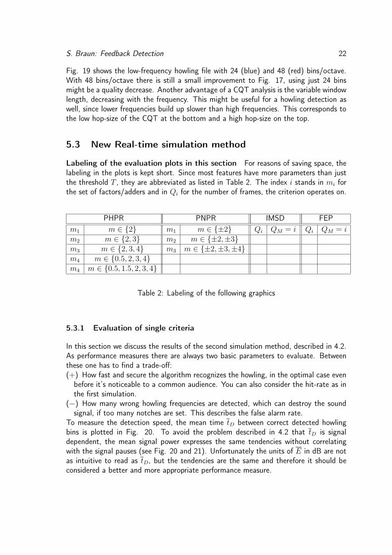
5.3 New Real-time simulation method

Labeling of the evaluation plots in this section For reasons of saving space, thelabeling in the plots is kept short. Since most features have more parameters than justthe threshold T , they are abbreviated as listed in Table 2. The index i stands in mi forthe set of factors/adders and in Qi for the number of frames, the criterion operates on.

PHPR PNPR IMSD FEPm1 m ∈ {2} m1 m ∈ {±2} Qi QM = i Qi QM = im2 m ∈ {2, 3} m2 m ∈ {±2,±3}m3 m ∈ {2, 3, 4} m3 m ∈ {±2,±3,±4}m4 m ∈ {0.5, 2, 3, 4}m4 m ∈ {0.5, 1.5, 2, 3, 4}

Table 2: Labeling of the following graphics

5.3.1 Evaluation of single criteria

In this section we discuss the results of the second simulation method, described in 4.2.As performance measures there are always two basic parameters to evaluate. Betweenthese one has to find a trade-off:(+) How fast and secure the algorithm recognizes the howling, in the optimal case even

before it’s noticeable to a common audience. You can also consider the hit-rate as inthe first simulation.

(−) How many wrong howling frequencies are detected, which can destroy the soundsignal, if too many notches are set. This describes the false alarm rate.

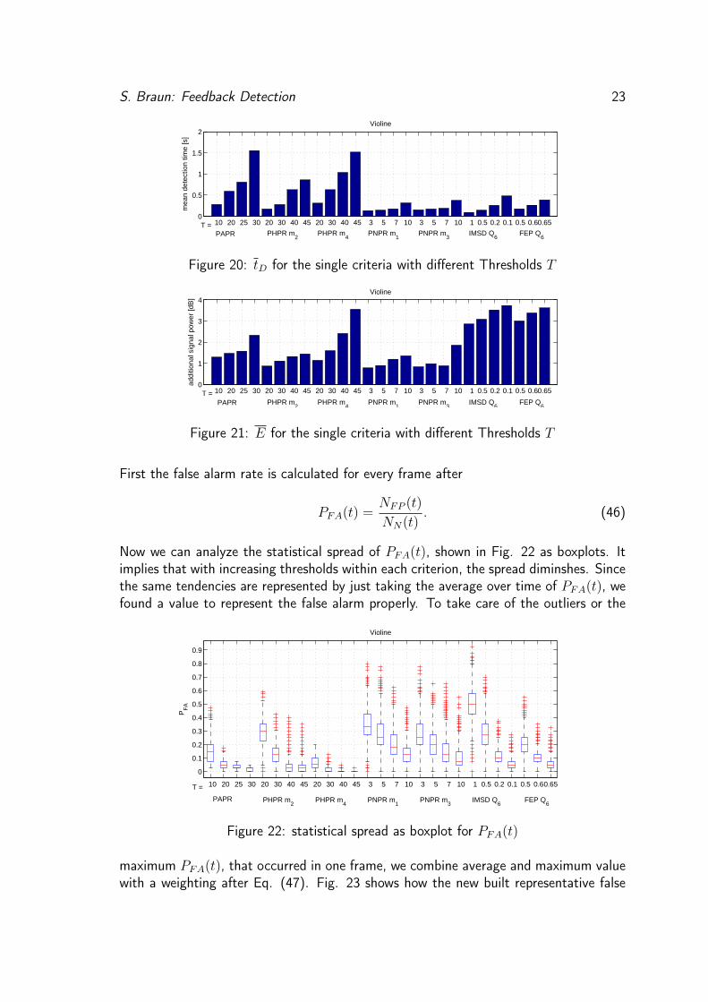
To measure the detection speed, the mean time tD between correct detected howlingbins is plotted in Fig. 20. To avoid the problem described in 4.2 that tD is signaldependent, the mean signal power expresses the same tendencies without correlatingwith the signal pauses (see Fig. 20 and 21). Unfortunately the units of E in dB are notas intuitive to read as tD, but the tendencies are the same and therefore it should beconsidered a better and more appropriate performance measure.


10 20 25 30 20 30 40 45 20 30 40 45 3 5 7 10 3 5 7 10 1 0.5 0.2 0.1 0.5 0.60.650

0.5

1

1.5

2Violine

mea

n de

tect

ion

time

[s]

T =PAPR PHPR m

2PHPR m

4PNPR m

1PNPR m

3IMSD Q

6FEP Q

6

Figure 20: tD for the single criteria with different Thresholds T

10 20 25 30 20 30 40 45 20 30 40 45 3 5 7 10 3 5 7 10 1 0.5 0.2 0.1 0.5 0.60.650

1

2

3

4

addi

tiona

l sig

nal p

ower

[dB

]

Violine

T =PAPR PHPR m

2PHPR m

4PNPR m

1PNPR m

3IMSD Q

6FEP Q

6

Figure 21: E for the single criteria with different Thresholds T

First the false alarm rate is calculated for every frame after

PFA(t) =NFP (t)

NN(t). (46)

Now we can analyze the statistical spread of PFA(t), shown in Fig. 22 as boxplots. Itimplies that with increasing thresholds within each criterion, the spread diminshes. Sincethe same tendencies are represented by just taking the average over time of PFA(t), wefound a value to represent the false alarm properly. To take care of the outliers or the

10 20 25 30 20 30 40 45 20 30 40 45 3 5 7 10 3 5 7 10 1 0.5 0.2 0.1 0.5 0.60.65

0

0.1

0.2

0.3

0.4

0.5

0.6

0.7

0.8

0.9

PF

A

Violine

T =

PAPR PHPR m2

PHPR m4

PNPR m1

PNPR m3

IMSD Q6

FEP Q6

Figure 22: statistical spread as boxplot for PFA(t)

maximum PFA(t), that occurred in one frame, we combine average and maximum valuewith a weighting after Eq. (47). Fig. 23 shows how the new built representative false


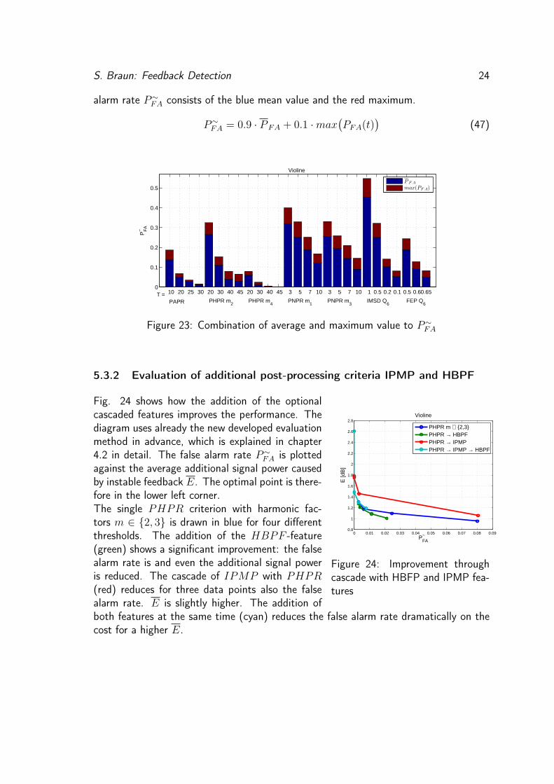
alarm rate P∼FA consists of the blue mean value and the red maximum.

P∼FA = 0.9 · P FA + 0.1 ·max

(PFA(t)

)(47)

10 20 25 30 20 30 40 45 20 30 40 45 3 5 7 10 3 5 7 10 1 0.5 0.2 0.1 0.5 0.60.650

0.1

0.2

0.3

0.4

0.5

Violine

PF

A~

T =PAPR PHPR m

2PHPR m

4PNPR m

1PNPR m

3IMSD Q

6FEP Q

6

PF A

max(PF A)

Figure 23: Combination of average and maximum value to P∼FA

5.3.2 Evaluation of additional post-processing criteria IPMP and HBPF

0 0.01 0.02 0.03 0.04 0.05 0.06 0.07 0.08 0.090.8

1

1.2

1.4

1.6

1.8

2

2.2

2.4

2.6

2.8

PFA~

E [d

B]

Violine

PHPR m ∈ {2,3}PHPR → HBPFPHPR → IPMPPHPR → IPMP → HBPF

Figure 24: Improvement throughcascade with HBFP and IPMP fea-tures

Fig. 24 shows how the addition of the optionalcascaded features improves the performance. Thediagram uses already the new developed evaluationmethod in advance, which is explained in chapter4.2 in detail. The false alarm rate P∼

FA is plottedagainst the average additional signal power causedby instable feedback E. The optimal point is there-fore in the lower left corner.The single PHPR criterion with harmonic fac-tors m ∈ {2, 3} is drawn in blue for four differentthresholds. The addition of the HBPF -feature(green) shows a significant improvement: the falsealarm rate is and even the additional signal poweris reduced. The cascade of IPMP with PHPR(red) reduces for three data points also the falsealarm rate. E is slightly higher. The addition ofboth features at the same time (cyan) reduces the false alarm rate dramatically on thecost for a higher E.


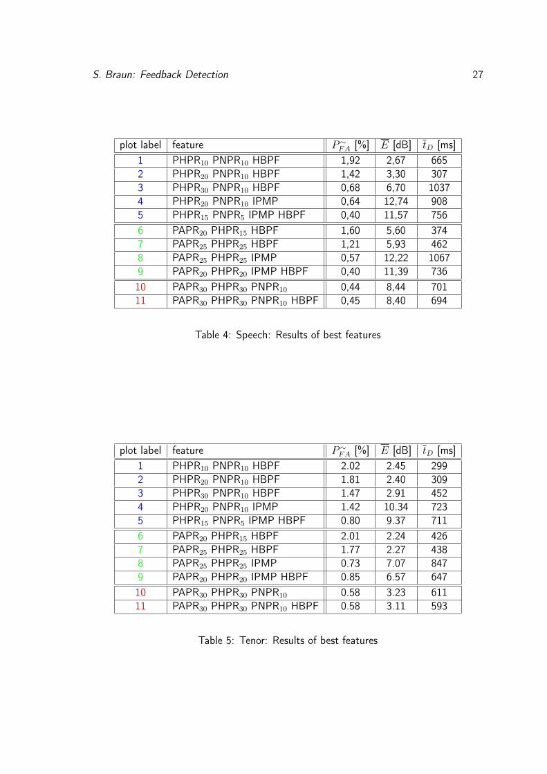
5.3.3 Comparison and evaluation of the best performing features

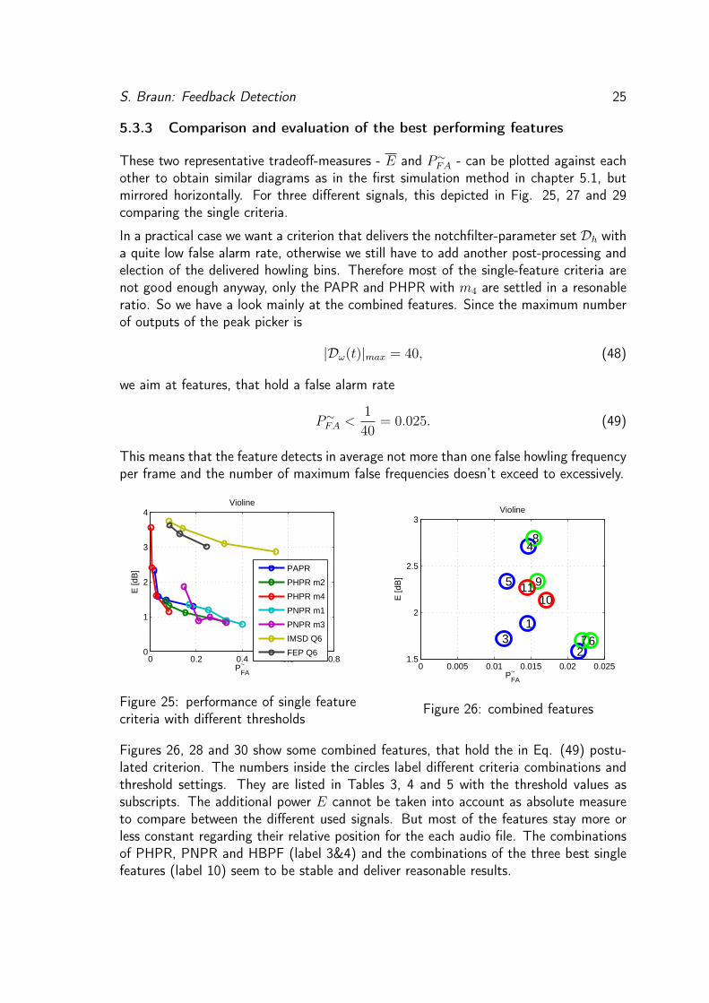
These two representative tradeoff-measures - E and P∼FA - can be plotted against each

other to obtain similar diagrams as in the first simulation method in chapter 5.1, butmirrored horizontally. For three different signals, this depicted in Fig. 25, 27 and 29comparing the single criteria.

In a practical case we want a criterion that delivers the notchfilter-parameter set Dh witha quite low false alarm rate, otherwise we still have to add another post-processing andelection of the delivered howling bins. Therefore most of the single-feature criteria arenot good enough anyway, only the PAPR and PHPR with m4 are settled in a resonableratio. So we have a look mainly at the combined features. Since the maximum numberof outputs of the peak picker is

|Dω(t)|max = 40, (48)

we aim at features, that hold a false alarm rate

P∼FA <

1

40= 0.025. (49)

This means that the feature detects in average not more than one false howling frequencyper frame and the number of maximum false frequencies doesn’t exceed to excessively.

0 0.2 0.4 0.6 0.80

1

2

3

4

PFA~

E [d

B]

Violine

PAPR

PHPR m2

PHPR m4

PNPR m1

PNPR m3

IMSD Q6

FEP Q6

Figure 25: performance of single featurecriteria with different thresholds

0 0.005 0.01 0.015 0.02 0.0251.5

2

2.5

3

PFA~

E [d

B]

Violine

1

2 3

4

5

6 7

8

9

1011

Figure 26: combined features

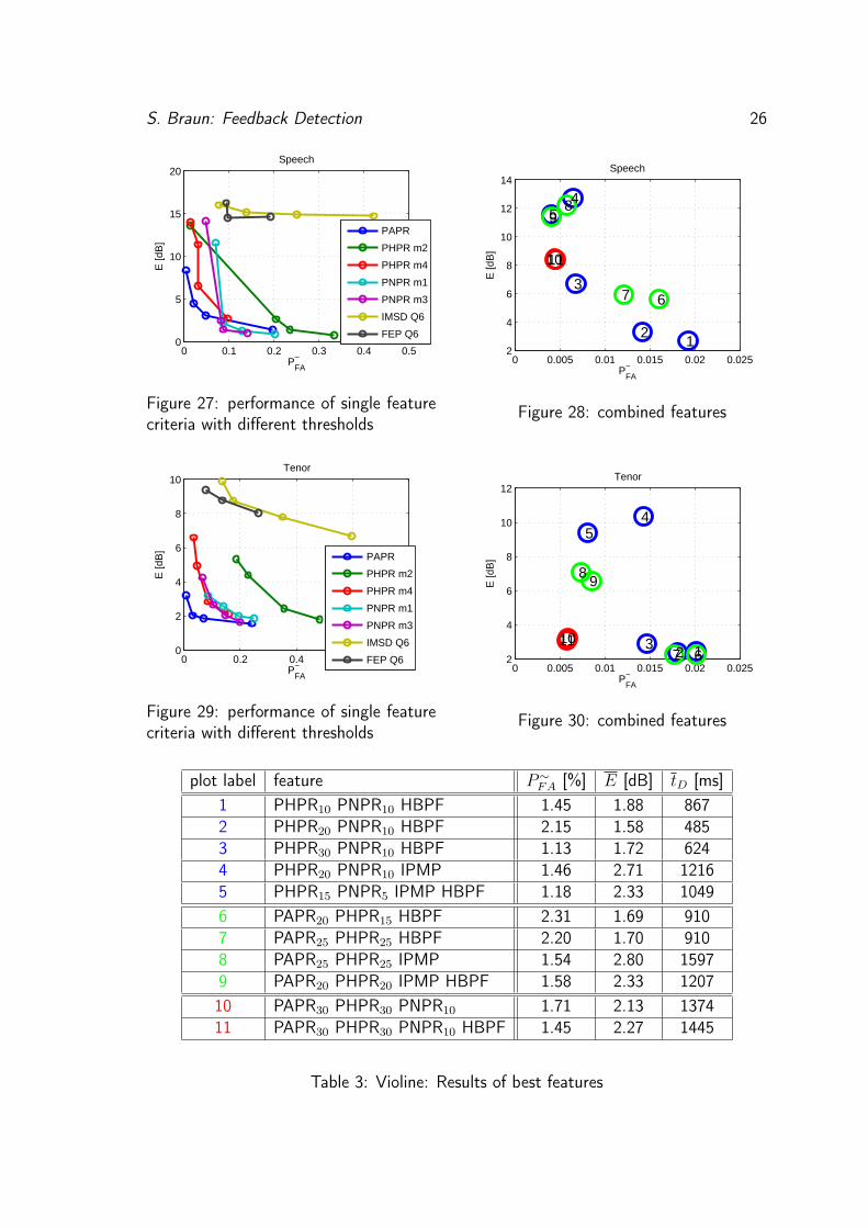
Figures 26, 28 and 30 show some combined features, that hold the in Eq. (49) postu-lated criterion. The numbers inside the circles label different criteria combinations andthreshold settings. They are listed in Tables 3, 4 and 5 with the threshold values assubscripts. The additional power E cannot be taken into account as absolute measureto compare between the different used signals. But most of the features stay more orless constant regarding their relative position for the each audio file. The combinationsof PHPR, PNPR and HBPF (label 3&4) and the combinations of the three best singlefeatures (label 10) seem to be stable and deliver reasonable results.


0 0.1 0.2 0.3 0.4 0.50

5

10

15

20

PFA~

E [d

B]

Speech

PAPR

PHPR m2

PHPR m4

PNPR m1

PNPR m3

IMSD Q6

FEP Q6


0 0.005 0.01 0.015 0.02 0.0252

4

6

8

10

12

14

PFA~

E [d

B]

Speech

1 2

3

4 5

6 7

8 9

1011


0 0.2 0.4 0.6 0.80

2

4

6

8

10

PFA~

E [d

B]

Tenor

PAPR

PHPR m2

PHPR m4

PNPR m1

PNPR m3

IMSD Q6

FEP Q6


0 0.005 0.01 0.015 0.02 0.0252

4

6

8

10

12

PFA~

E [d

B]

Tenor

1 2 3

4 5

6 7

8 9

1011


plot label feature P∼FA [%] E [dB] tD [ms]

1 PHPR10 PNPR10 HBPF 1.45 1.88 8672 PHPR20 PNPR10 HBPF 2.15 1.58 4853 PHPR30 PNPR10 HBPF 1.13 1.72 6244 PHPR20 PNPR10 IPMP 1.46 2.71 12165 PHPR15 PNPR5 IPMP HBPF 1.18 2.33 10496 PAPR20 PHPR15 HBPF 2.31 1.69 9107 PAPR25 PHPR25 HBPF 2.20 1.70 9108 PAPR25 PHPR25 IPMP 1.54 2.80 15979 PAPR20 PHPR20 IPMP HBPF 1.58 2.33 120710 PAPR30 PHPR30 PNPR10 1.71 2.13 137411 PAPR30 PHPR30 PNPR10 HBPF 1.45 2.27 1445

Table 3: Violine: Results of best features



1 PHPR10 PNPR10 HBPF 1,92 2,67 6652 PHPR20 PNPR10 HBPF 1,42 3,30 3073 PHPR30 PNPR10 HBPF 0,68 6,70 10374 PHPR20 PNPR10 IPMP 0,64 12,74 9085 PHPR15 PNPR5 IPMP HBPF 0,40 11,57 7566 PAPR20 PHPR15 HBPF 1,60 5,60 3747 PAPR25 PHPR25 HBPF 1,21 5,93 4628 PAPR25 PHPR25 IPMP 0,57 12,22 10679 PAPR20 PHPR20 IPMP HBPF 0,40 11,39 73610 PAPR30 PHPR30 PNPR10 0,44 8,44 70111 PAPR30 PHPR30 PNPR10 HBPF 0,45 8,40 694

Table 4: Speech: Results of best features


1 PHPR10 PNPR10 HBPF 2.02 2.45 2992 PHPR20 PNPR10 HBPF 1.81 2.40 3093 PHPR30 PNPR10 HBPF 1.47 2.91 4524 PHPR20 PNPR10 IPMP 1.42 10.34 7235 PHPR15 PNPR5 IPMP HBPF 0.80 9.37 7116 PAPR20 PHPR15 HBPF 2.01 2.24 4267 PAPR25 PHPR25 HBPF 1.77 2.27 4388 PAPR25 PHPR25 IPMP 0.73 7.07 8479 PAPR20 PHPR20 IPMP HBPF 0.85 6.57 64710 PAPR30 PHPR30 PNPR10 0.58 3.23 61111 PAPR30 PHPR30 PNPR10 HBPF 0.58 3.11 593

Table 5: Tenor: Results of best features


5.4 Subjective evaluation with PD patch

A patch is developed in Pure Data for a real-time subjective evaluation. Two optionscorresponding to the evaluation methods are available:– Feedback_Detection_only.pd: A “static” implementation, where a audiofile con-

taining a growing howling component is played back. The algorithm detects thehowling and attenuates it down via notchfilters.

– fb_sim_and_cancel.pd: A “dynamic” implementation containing a feedback loopwith a measured room impulse response. After having chosen the algorithm andsetting it up, a signal can be played back through a feedback loop. By turning upthe feedback gain, the system starts to get unstable and to howl. If the algorithm isset up properly it will detect the howling and set a notchfilter, so that the system isstable again.

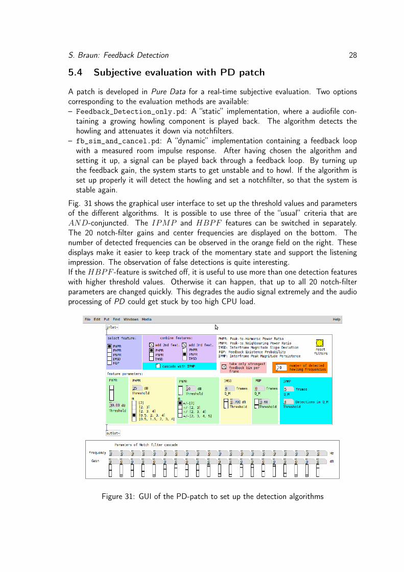
Fig. 31 shows the graphical user interface to set up the threshold values and parametersof the different algorithms. It is possible to use three of the “usual” criteria that areAND-conjuncted. The IPMP and HBPF features can be switched in separately.The 20 notch-filter gains and center frequencies are displayed on the bottom. Thenumber of detected frequencies can be observed in the orange field on the right. Thesedisplays make it easier to keep track of the momentary state and support the listeningimpression. The observation of false detections is quite interesting.If the HBPF -feature is switched off, it is useful to use more than one detection featureswith higher threshold values. Otherwise it can happen, that up to all 20 notch-filterparameters are changed quickly. This degrades the audio signal extremely and the audioprocessing of PD could get stuck by too high CPU load.

Figure 31: GUI of the PD-patch to set up the detection algorithms


Notch-filter design The control and design algorithm for the bank of 20 notch-filtersis kept as simple as possible. Nevertheless, it this algorithm is essential for a subjectivegood performance of the howling canceller, so some tweaks are listed here.– Blocksize: N = 2048 samples, N/2 overlapping, fs = 441001

s.

– Fixed notch-filter bandwidth: 130

octave.– If a frequency is within the bandwidth, where already a notchfilter was or is set, the

same existing filter with its center frequency unchanged is used.– Gain-reduction value: -3 dB. Everytime a new or before existing howling frequency

is detected, the corresponding notch-filter gain is reduced by -3 dB until a maximumvalue of -30 dB.

– Gain-make-up value: +2 dB. If a notch-filter gain was not reduced for some consec-utive frames, the filter gain is made up by +2 dB again until it reaches 0 dB or isreduced again.

– Time constant: 2 sec. Make-up gain by +2 dB after 10 frames, if no correspondinghowling frequency is detected.

This design ensures a smooth operation of not too fast gain reductions, which can annoythe listener. After some time, notch-filters are taken out again, if they are not neededanymore. This can be due to a change of the room situation. If a feedback frequencywould be always present, it levels to a stable reduction value.

6 Conclusion and outlook

By implementing and examinating the most common feedback howling detection crite-ria, a good overview of the state of the art is gathered. A new, more stable methodfor evaluation is developed and applied. Moreover, a method to estimate the feedbackloop gain by using a second microhpone is proposed, but could not be tested sufficientlywithin the framework of this work.The most effective algorithms focus on the short-time spectrum. The incorporation oftemporal features gives a little more stability (i.e. reduction of false alarm), but at thecost of a much slower reaction time.

To get a perceptual motivated evaluation of the algorithms, a subjective listening testshould be considered for future work. But that includes also strongly the notch-filtercontrolling and design. The effects of spectral distortion by setting unneeded notch-filters is an important information to design a good algorithm. Since the algorithms arecoded in Matlab and Pure Data, they can form the basis of a following research anddevelop a more advanced method to control and design the notch-filter parameters.


References

[1] Waterschoot, Toon van and Moonen, Marc: “50 Years of Acoustic Feedback Con-trol: State of the Art and Future Challenges”, Proc. IEEE, vol. 99, no. 2, Feb.2011, pp. 288-327.

[2] Waterschoot, Toon van & Moonen, Marc: “Comparative evaluation of howlingdetection criteria in notch-filter-based howling suppression”, AES Journal vol. 58,no. 11, Leuven, 2010

[3] J. C. Brown, “Calculation of a constant Q spectral transform“, J. Acoust. Soc.Am., vol. 89, no. 1, pp. 425-434, 1991.

[4] J. C. Brown and M. S. Puckette, ”An efficient algorithm for the calculation of aconstant Q transform“, J. Acoust. Soc. Am., vol. 92, no. 5, pp. 2698-2701, 1992.

[5] Schörkhuber, Christian and Klapuri, Anssi: ”Constant-Q Transform Toolbox forMusic Processing“, 7th Sound and Music Computing Conference, Barcelona, Spain,2010.

[6] N. Osmanovic, V. E. Clarke, and E. Velandia, ”An In-Flight Low Latency AcousticFeedback Cancellation Algorithm“,123rd AES Convention, J. Audio Eng. Soc., 2007Oct., convention paper 7266.

[7] Horn, Martin and Dourdoumas, Nicolaos, ”Regelungstechnik“, Pearson Studium,München 2004.

Documents

Evaluation of various Algorithms to detect acoustic Feedback · PDF fileS. Braun: Feedback Detection 3 ... frequencies between about 200 and 5000 Hz . The howling has a very narrow-band