Evaluation of Ultrasonic Snow Depth Sensors for U.S. Snow ...ccc.atmos.colostate.edu/pdfs/...etal-evaluating_snow_depth_sensors.pdf · Evaluation of Ultrasonic Snow Depth Sensors

Evaluation of Ultrasonic Snow Depth Sensors for U.S. Snow Measurements

WENDY A. RYAN AND NOLAN J. DOESKEN

Department of Atmospheric Science, Colorado State University, Fort Collins, Colorado

STEVEN R. FASSNACHT

Watershed Science Program, Colorado State University, Fort Collins, Colorado

(Manuscript received 1 December 2006, in final form 12 September 2007)

ABSTRACT

Ultrasonic snow depth sensors are examined as a low cost, automated method to perform traditional snowmeasurements. In collaboration with the National Weather Service, nine sites across the United States wereequipped with two manufacturers of ultrasonic depth sensors: the Campbell Scientific SR-50 and the JuddCommunications sensor. Following standard observing protocol, manual measurements of 6-h snowfall andtotal snow depth on ground were also gathered. Results show that the sensors report the depth of snowdirectly beneath on average within �1 cm of manual observations. However, the sensors tended to under-estimate the traditional total depth of snow-on-ground measurement by approximately 2 cm. This is mainlyattributed to spatial variability of the snow cover caused by factors such as wind scour and wind drift.

After assessing how well the sensors represented the depth of snow on the ground, two algorithms werecreated to estimate the traditional measurement of 6-h snowfall from the continuous snow depth reportedby the sensors. A 5-min snowfall algorithm (5MSA) and a 60-min snowfall algorithm (60MSA) werecreated. These simple algorithms essentially sum changes in snow depth using 5- and 60-min intervals ofchange and sum positive changes over the traditional 6-h observation periods after compaction routines areapplied. The algorithm results were compared to manual observations of snowfall. The results indicated thatthe 5MSA worked best with the Campbell Scientific sensor. The Campbell sensor appears to estimatesnowfall more accurately than the Judd sensor due to the difference in sensor resolution. The Judd sensorresults did improve with the 60-min snowfall algorithm. This technology does appear to have potential forcollecting useful and timely information on snow accumulation, but determination of snowfall to the currentrequirement of 0.1 in. (0.25 cm) is a difficult task.

1. Introduction

Snowfall and snow depth measurements are impor-tant to a variety of disciplines including commerce,transportation, winter recreation, and water supplyforecasting. The western United States depends onsnowfall for 75% of their annual water supply(Doesken and Judson 1997). For most of the UnitedStates outside of the high, mountainous regions of theWest, the National Weather Service (NWS) is the pri-mary source for snow measurements. Surface observa-tions available from the NWS currently include severalhundred airport weather stations across the country

where observations of many weather elements aretransmitted hourly. This network is supplemented byNWS historic Cooperative Observer Network (NRC1998) with several thousand weather stations measuringtemperature and precipitation once daily. In the early1990s the NWS began deploying the Automated Sur-face Observing System (ASOS) at major U.S. airportsin conjunction with the Federal Aviation Administra-tion and the Department of Defense. The ASOS mea-sures a variety of meteorological components includingtemperature, humidity, wind speed and direction, pre-cipitation amounts, presence and type of precipitation,sky condition, visibility and obstructions to vision, andbarometric pressure. ASOS does not measure tradi-tional snow parameters, except for the liquid equivalentof snow. Since its beginning, ASOS has used a heatedtipping-bucket rain gauge to record precipitation in-cluding rain and the water content of solid precipitation

Corresponding author address: Wendy A. Ryan, 1371 GeneralDelivery, Colorado State University, Fort Collins, CO 80523-1371.E-mail: [email protected]

MAY 2008 R Y A N E T A L . 667

DOI: 10.1175/2007JTECHA947.1

© 2008 American Meteorological Society

JTECHA947

(Doesken and McKee 1999). The use of this type ofgauge creates problems of underreporting precipita-tion particularly for snow falling at temperatures sev-eral degrees below freezing (Doesken and McKee1999). However, ASOS is now converting the precipi-tation gauge to the all-weather precipitation gauge(AWPAG), which is a weighing-type gauge and morecapable of measuring nonliquid precipitation (NWS2004).

Prior to the recent deployment of ASOS, many citieshad snowfall records dating back to the late 1800s.Many of these long-term snowfall station records werediscontinued or transferred to stations some distanceaway that may not be representative (McKee et al.2000). There is a definite need and interest in qualitylong-term snowfall records in the United States, yetRobinson (1989), who studied historic snowfall records,found that there are very few locations across the coun-try with complete and accurate snow measurementrecords. Implementation of ASOS further magnifiedthis problem. An ongoing study of snowfall trends inthe United States has documented decades of observa-tional inconsistency, even when only manual observa-tions at long-term stations are considered (Kunkel et al.2007). This study aims to evaluate the use of ultrasonicsnow depth sensors to restore snowfall and snow depthmeasurements at ASOS and other automated stationsand to potentially achieve a higher degree of data con-tinuity.

a. Traditional snow measurements

The traditional NWS snow measurements consistedof gauge precipitation, snowfall, snow depth, and (at asubset of stations) snow water equivalent (SWE).Gauge precipitation is defined as the amount of liquidequivalent obtained by an NWS nonrecording, stan-dard precipitation gauge (NWS 2006). Snowfall is de-fined as the maximum accumulation of new snow sincethe last observation and is customarily measured manu-ally with a ruler on a snow measurement board. Themeasurement board is cleared after each observation.Snow depth is defined as the total depth of snow on theground at the time of observation and includes both oldand new snow on undisturbed surfaces. The measure-ment of snow depth may be the average of several totaldepth measurements to obtain a representative sample(NWS 1996). Gauge precipitation is measured to thehundredth of an inch, snowfall is measured to the tenthof an inch, and total snow depth is observed to thewhole inch. Airport weather stations traditionally mea-sured snowfall every 6 h, while Cooperative ObserverNetwork stations typically measure once a day.

This evaluation of ultrasonic snow depth sensors for

measuring total depth of snow on ground and freshsnowfall estimation from changes in total snow depth isdone with respect to manual measurements assumed tobe “ground truth.” Uniformity and consistency inmanual measurements were strongly encouraged withinthe team of cooperators who helped collect data fromour test sites. However, there is inherent uncertainty inmanual measurements due to the fact that snow melts,settles, blows, and drifts and does not accumulate uni-formly on the ground. Depending on the time of day,the frequency, the measurement surface (i.e., grass,snow measurement board, etc.), the extent of nonuni-formity in snow accumulation, and the overall care anddetail of the individual observers, variability in manualobservations must be expected. The authors are notaware of studies that have quantified this uncertainty interms of measurement error, but would easily expect itto be in the magnitude of �25%. The authors will quan-tify this in future research as it is not in the scope of thecurrent study; however, it will impact a transition frommanual to automated snow measurements.

b. Ultrasonic snow depth sensors

Ultrasonic depth sensors (USDS) have been underdevelopment since the early 1980s (Goodison et al.1984) with recent implementation into the Snow Te-lemetry (SNOTEL) network (Lea and Lea 1998).These sensors send out an ultrasonic (50 kHz) soundpulse and measure the time it takes to reach the groundor snow surface and reflect back to the sensor. Theultrasonic pulse projects downward over a cone of 22°(Fig. 1). It is important to ensure that there is no inter-ference with the 22° cone such as trees, wires, installa-tion hardware, etc. The time for the pulse to return tothe transducer is adjusted for the speed of sound in airbased on measured air temperature, and the timing isconverted to a distance via internal algorithms.

To adjust the speed of sound in air (Vsound) in metersper second for the ambient air temperature (Ta) inkelvins, Eq. (1.1) is used:

Vsound � 331.4�Ta �273.15�0.5. �1.1�

The distance the sound pulse travels decreases as snowaccumulates on the ground, thus reducing the time forthe pulse to return to the sensor.

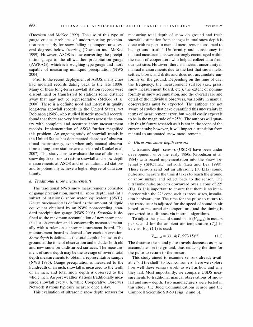
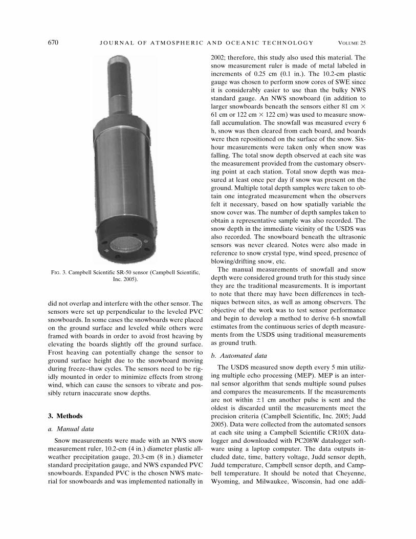
This study aimed to examine sensors already avail-able “off the shelf” to local consumers. Here we explorehow well these sensors work, as well as how and whythey fail. Most importantly, we compare USDS mea-surements to traditional manual observations of snow-fall and snow depth. Two manufacturers were tested inthis study, the Judd Communications sensor and theCampbell Scientific SR-50 (Figs. 2 and 3).

668 J O U R N A L O F A T M O S P H E R I C A N D O C E A N I C T E C H N O L O G Y VOLUME 25

2. Study sites

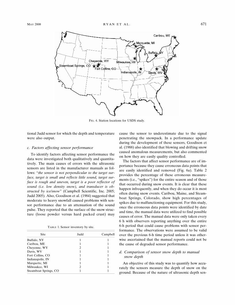
This research project included nine sites (Fig. 4)throughout the coterminous United States that testedboth the Judd Communications and Campbell Scien-tific depth sensors with manual measurements duringthe 2004/05 snow season (Table 1). Additional siteswere a part of the study, but only those stations whereJudd, Campbell, and manual observations were takencoincidently will be shown here. Six sites were locatedat NWS forecast offices. The Davis, West Virginia, site

was an NWS Cooperative site whose observer volun-teered for the project. Other non-NWS sites were FortCollins and Steamboat Springs, Colorado. Sites werechosen on willingness to participate, although theamount of snow historically received was also takeninto account. Because of technical problems, the use ofthe data from Caribou, Maine, and Indianapolis, Indi-ana, are limited.

The siting of USDS is very important to achievingquality data. A site sheltered from wind effects (i.e., aforested clearing) would be an ideal condition; how-ever, this is rarely available. Each individual site wasresponsible for mounting and installing the sensors andplacing them as close to the customary observing pointas possible to ensure similar exposure. The basic setupwas similar for each site (Fig. 5).

The sensors were calibrated to read zero snow depthon a level, white expanded polyvinylchloride (PVC)snowboard under snow-free conditions. Snowboardsizes were either 81 cm � 61 cm or 122 cm � 122 cmdepending on the height the sensors were mounted offthe ground. Different sizes were used to ensure the 22°cone was completely within the bounds of the snow-boards. Sensors were mounted perpendicular to thesurface of interest at a height of 0.5 to 10 m off theground depending on the historic maximum snow depthat each location. The sensors were mounted as close aspossible to each other in order to minimize spatial vari-ability and allow direct comparison of measurements.The sensors also needed to be far enough apart that the22° cone of influence utilized by the ultrasonic pulsesFIG. 2. Judd Communications depth sensor (Judd 2005).

FIG. 1. Diagram showing the 22° cone utilized by the ultrasonic sensors (Judd 2005).

MAY 2008 R Y A N E T A L . 669

did not overlap and interfere with the other sensor. Thesensors were set up perpendicular to the leveled PVCsnowboards. In some cases the snowboards were placedon the ground surface and leveled while others wereframed with boards in order to avoid frost heaving byelevating the boards slightly off the ground surface.Frost heaving can potentially change the sensor toground surface height due to the snowboard movingduring freeze–thaw cycles. The sensors need to be rig-idly mounted in order to minimize effects from strongwind, which can cause the sensors to vibrate and pos-sibly return inaccurate snow depths.

3. Methods

a. Manual data

Snow measurements were made with an NWS snowmeasurement ruler, 10.2-cm (4 in.) diameter plastic all-weather precipitation gauge, 20.3-cm (8 in.) diameterstandard precipitation gauge, and NWS expanded PVCsnowboards. Expanded PVC is the chosen NWS mate-rial for snowboards and was implemented nationally in

2002; therefore, this study also used this material. Thesnow measurement ruler is made of metal labeled inincrements of 0.25 cm (0.1 in.). The 10.2-cm plasticgauge was chosen to perform snow cores of SWE sinceit is considerably easier to use than the bulky NWSstandard gauge. An NWS snowboard (in addition tolarger snowboards beneath the sensors either 81 cm �61 cm or 122 cm � 122 cm) was used to measure snow-fall accumulation. The snowfall was measured every 6h, snow was then cleared from each board, and boardswere then repositioned on the surface of the snow. Six-hour measurements were taken only when snow wasfalling. The total snow depth observed at each site wasthe measurement provided from the customary observ-ing point at each station. Total snow depth was mea-sured at least once per day if snow was present on theground. Multiple total depth samples were taken to ob-tain one integrated measurement when the observersfelt it necessary, based on how spatially variable thesnow cover was. The number of depth samples taken toobtain a representative sample was also recorded. Thesnow depth in the immediate vicinity of the USDS wasalso recorded. The snowboard beneath the ultrasonicsensors was never cleared. Notes were also made inreference to snow crystal type, wind speed, presence ofblowing/drifting snow, etc.

The manual measurements of snowfall and snowdepth were considered ground truth for this study sincethey are the traditional measurements. It is importantto note that there may have been differences in tech-niques between sites, as well as among observers. Theobjective of the work was to test sensor performanceand begin to develop a method to derive 6-h snowfallestimates from the continuous series of depth measure-ments from the USDS using traditional measurementsas ground truth.

b. Automated data

The USDS measured snow depth every 5 min utiliz-ing multiple echo processing (MEP). MEP is an inter-nal sensor algorithm that sends multiple sound pulsesand compares the measurements. If the measurementsare not within �1 cm another pulse is sent and theoldest is discarded until the measurements meet theprecision criteria (Campbell Scientific, Inc. 2005; Judd2005). Data were collected from the automated sensorsat each site using a Campbell Scientific CR10X data-logger and downloaded with PC208W datalogger soft-ware using a laptop computer. The data outputs in-cluded date, time, battery voltage, Judd sensor depth,Judd temperature, Campbell sensor depth, and Camp-bell temperature. It should be noted that Cheyenne,Wyoming, and Milwaukee, Wisconsin, had one addi-

FIG. 3. Campbell Scientific SR-50 sensor (Campbell Scientific,Inc. 2005).


tional Judd sensor for which the depth and temperaturewere also output.

c. Factors affecting sensor performance

To identify factors affecting sensor performance thedata were investigated both qualitatively and quantita-tively. The main causes of errors with the ultrasonicsensors are listed in the manufacturer manuals as fol-lows: “the sensor is not perpendicular to the target sur-face, target is small and reflects little sound, target sur-face is rough and uneven, target is a poor reflector ofsound (i.e. low density snow), and transducer is ob-structed by ice/snow” (Campbell Scientific, Inc. 2005;Judd 2005). Also, Goodison et al. (1984) suggested thatmoderate to heavy snowfall caused problems with sen-sor performance due to an attenuation of the soundpulse. They reported that the surface of the snow struc-ture (loose powder versus hard packed crust) may

cause the sensor to underestimate due to the signalpenetrating the snowpack. In a performance updateduring the development of these sensors, Goodison etal. (1988) also identified that blowing and drifting snowcaused anomalous measurements, but also commentedon how they are easily quality controlled.

The factors that affect sensor performance are of im-portance because they cause erroneous data points thatare easily identified and removed (Fig. 6a). Table 2provides the percentage of these erroneous measure-ments (i.e., “spikes”) for the entire season and of thosethat occurred during snow events. It is clear that thesehappen infrequently, and when they do occur it is mostoften during snow events. Caribou, Maine, and Steam-boat Springs, Colorado, show high percentages ofspikes due to malfunctioning equipment. For this study,once the erroneous data points were identified by dateand time, the manual data were utilized to find possiblecauses of error. The manual data were only taken every6 h with observers reporting anything over the entire6-h period that could cause problems with sensor per-formance. The observations were assumed to be validover the previous 6-h time period unless it was other-wise ascertained that the manual reports could not bethe cause of degraded sensor performance.

d. Comparison of sensor snow depth to manualsnow depth

An objective of this study was to quantify how accu-rately the sensors measure the depth of snow on theground. Because of the nature of ultrasonic depth sen-

TABLE 1. Sensor inventory by site.

Site Judd Campbell

Buffalo, NY 1 1Caribou, ME 1 1Cheyenne, WY 2 1Davis, WV 1 1Fort Collins, CO 1 1Indianapolis, IN 1 1Marquette, MI 1 1Milwaukee, WI 2 1Steamboat Springs, CO 1 1

FIG. 4. Station locations for USDS study.

MAY 2008 R Y A N E T A L . 671

sors having “noisy” data (Fig. 6b), moving averageswere applied to create a smooth snow depth time seriesfor comparison. Both 1- and 3-h moving averages wereapplied to the data to give a better understanding ofwhich amount of smoothing worked best for each sen-sor at each site. The main reason for the data smoothingwas the sensor data resolution, which for the Judd is 3mm (Judd 2005) and the Campbell 0.1 mm (CampbellScientific, Inc. 2005). The total depth of snow on theground can be an average of several depth measure-ments to obtain a representative measurement, if spa-tial variability is deemed present. To minimize the ef-fects of spatial variability, the snow depth on the boardsbeneath the sensors was also measured. Both of themeasurements were then paired with the USDS read-ing. To describe errors associated with both mea-surements the average difference, standard devia-tion of difference, mean absolute error, and root-mean-square errors (RMSEs) were calculated for eachcomparison. The root-mean-square error for themeasurements was normalized by the average snow

depth at each location (J. zumBrunnen, ColoradoState University, 2005, personal communication).This was done in order to compare the RMSE fromsite to site. For example, an RMSE at a site with 25 cmof annual snowfall is much more significant than thesame RMSE at a site receiving 150 cm of annual snow-fall.

e. Six-hour snowfall algorithm

To create a snowfall algorithm, 6-h snowfall was cal-culated from the 5-min sensor data. This calculationwas done using two different methods, a 5-min snowfallalgorithm and a 60-min snowfall algorithm. Using onlythe change in snow depth every 6 h would cause snow-fall to be omitted if it accumulated and melted withinthe 6-h period.

1) FIVE-MINUTE SNOWFALL ALGORITHM (5MSA)

The first method used a 5-min time step for calculat-ing snowfall according to Eq. (3.1) where t is time in

FIG. 5. Site photos: (a) Buffalo, NY; (b) Cheyenne, WY; and(c) Davis, WV.


minutes, i is time in hours, j is the number of 5-minintervals, and ds is snow depth. If the sensor snow depthincreased over the 5-min period the difference wastaken and called 5-min snowfall. If the depth did notincrease a zero was entered. The 5-min snowfall valueswere then summed over the 6-h observation intervalsused by each site to obtain the 5-min snowfall algorithmfor 6-h snowfall (6HSF5MSA):

6HSF5MSA � �i

i�6

�j�0

11

�dst�5� dst

� for all �dst�5� dst

� � 0.

�3.1�

2) SIXTY-MINUTE SNOWFALL ALGORITHM

(60MSA)

The second method took the change in snow depthover a 60-min interval according to Eq. (3.2). The posi-tive 60-min changes in snow depth were summed overthe 6-h observation periods to create the 60-min snow-fall algorithm for 6-h snowfall (6HSF60MSA):

6HSF60MSA � �i

i�6

�dst�60� dst

� for all �dst�60� dst

� � 0.

�3.2�

Both of these methods were performed on both 1-and 3-h moving averages in order to determine the ef-fect of smoothing as well as the degree of smoothingrequired by each sensor to accurately estimate 6-hsnowfall.

3) COMPACTION

Both of the above methods calculated snowfall oversmall time periods that do not take into account com-paction of the snowpack over the longer 6-h period.Once the 6-h snowfall values were calculated, compac-tion by both metamorphism and overburden were con-sidered. Metamorphism takes into account the break-down of snow crystals resulting in a compacted snowdepth, while overburden considers the weight of newsnow overlying old snow. Temperature-based compac-tion equations were obtained from the SNTHERM.89one-dimensional snowpack model by Jordan (1991),who modified Anderson’s (1976) equations. This com-paction model was chosen since temperature wasreadily available.

TABLE 2. Percentage of data spikes for the entire season and those occurring during snow events.

Site Judd—entire season Judd—during snow Campbell—entire season Campbell—during snow

Buffalo, NY 0.26 40.40 0.01 100.00Caribou, ME 8.86 1.82 14.01 3.88Cheyenne, WY 0.00 55.00 0.00 0.00Davis, WV 0.04 94.44 0.00 0.00Fort Collins, CO 0.05 86.96 0.13 20.31Indianapolis, IN 0.00 0.00 0.00 0.00Marquette, MI 2.54 13.58 0.18 65.67Milwaukee, WI 0.00 4.17 0.00 0.00Steamboat Springs, CO 6.24 3.13 17.85 31.94

FIG. 6. Marquette, MI, example of raw sensor data (top) show-ing erroneous data points and (bottom) demonstrating normalvariation.

MAY 2008 R Y A N E T A L . 673

4) STATISTICS

The statistics used to describe how well the algo-rithms performed included percent difference in totalseasonal snowfall accumulation, a Nash–Sutcliffe R-squared (Nash and Sutcliffe 1970) on the cumulativeseasonal snowfall, and MAE on the incremental 6-hsnowfall measurements. The percent difference in sea-sonal totals describes how well the sensors did at mea-suring the total seasonal accumulations. The Nash–Sutcliffe R-squared described how well the cumulativesensor estimated snowfall modeled the cumulativemanual snowfall pattern. A perfect Nash–Sutcliffe R-squared is 1.0 with negative values indicating that theobserved mean manual 6-h snowfall is a better predic-tor than the model; it is a measure of the model effi-ciency. The MAE described how well the calculatedsensor 6-h snowfall values matched the manual 6-hsnowfall measurements. The errors of commission(CEs) and errors of omission (OEs) were also calcu-

lated to describe what proportion of time the algo-rithms correctly reported the occurrence or nonoccur-rence of snowfall. The CEs illustrate the proportion oftime the sensors reported snowfall when none was mea-sured manually. The OEs illustrate the proportion oftime the sensors reported no snowfall when snowfallwas measured manually.

4. Results

a. Comparison of automated and manual snow depth

1) SENSOR COMPARISON TO DEPTH AT SENSORS

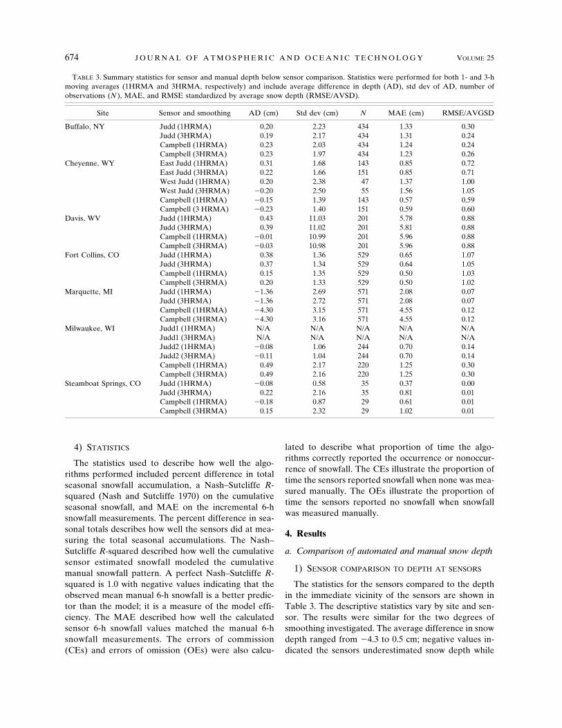
The statistics for the sensors compared to the depthin the immediate vicinity of the sensors are shown inTable 3. The descriptive statistics vary by site and sen-sor. The results were similar for the two degrees ofsmoothing investigated. The average difference in snowdepth ranged from �4.3 to 0.5 cm; negative values in-dicated the sensors underestimated snow depth while

TABLE 3. Summary statistics for sensor and manual depth below sensor comparison. Statistics were performed for both 1- and 3-hmoving averages (1HRMA and 3HRMA, respectively) and include average difference in depth (AD), std dev of AD, number ofobservations (N ), MAE, and RMSE standardized by average snow depth (RMSE/AVSD).

Site Sensor and smoothing AD (cm) Std dev (cm) N MAE (cm) RMSE/AVGSD

Buffalo, NY Judd (1HRMA) 0.20 2.23 434 1.33 0.30Judd (3HRMA) 0.19 2.17 434 1.31 0.24Campbell (1HRMA) 0.23 2.03 434 1.24 0.24Campbell (3HRMA) 0.23 1.97 434 1.23 0.26

Cheyenne, WY East Judd (1HRMA) 0.31 1.68 143 0.85 0.72East Judd (3HRMA) 0.22 1.66 151 0.85 0.71West Judd (1HRMA) 0.20 2.38 47 1.37 1.00West Judd (3HRMA) �0.20 2.50 55 1.56 1.05Campbell (1HRMA) �0.15 1.39 143 0.57 0.59Campbell (3 HRMA) �0.23 1.40 151 0.59 0.60

Davis, WV Judd (1HRMA) 0.43 11.03 201 5.78 0.88Judd (3HRMA) 0.39 11.02 201 5.81 0.88Campbell (1HRMA) �0.01 10.99 201 5.96 0.88Campbell (3HRMA) �0.03 10.98 201 5.96 0.88

Fort Collins, CO Judd (1HRMA) 0.38 1.36 529 0.65 1.07Judd (3HRMA) 0.37 1.34 529 0.64 1.05Campbell (1HRMA) 0.15 1.35 529 0.50 1.03Campbell (3HRMA) 0.20 1.33 529 0.50 1.02

Marquette, MI Judd (1HRMA) �1.36 2.69 571 2.08 0.07Judd (3HRMA) �1.36 2.72 571 2.08 0.07Campbell (1HRMA) �4.30 3.15 571 4.55 0.12Campbell (3HRMA) �4.30 3.16 571 4.55 0.12

Milwaukee, WI Judd1 (1HRMA) N/A N/A N/A N/A N/AJudd1 (3HRMA) N/A N/A N/A N/A N/AJudd2 (1HRMA) �0.08 1.06 244 0.70 0.14Judd2 (3HRMA) �0.11 1.04 244 0.70 0.14Campbell (1HRMA) 0.49 2.17 220 1.25 0.30Campbell (3HRMA) 0.49 2.16 220 1.25 0.30

Steamboat Springs, CO Judd (1HRMA) �0.08 0.58 35 0.37 0.00Judd (3HRMA) 0.22 2.16 35 0.81 0.01Campbell (1HRMA) �0.18 0.87 29 0.61 0.01Campbell (3HRMA) 0.15 2.32 29 1.02 0.01


positive values indicated they overestimated. The stan-dard deviation of average difference ranged from 0.58to 11 cm. The mean absolute error (MAE) ranged from0.37 to 6.0 cm. The normalized RMSE ranged from 0to 1.1.

Figure 7 shows plots of Buffalo, New York, sensorsnow depth plotted with manual snow depth next toeach sensor. Both sensors overestimated the observed

depth by an average of 0.2 cm with a standard deviationof 2.2 cm for the Judd and 2.0 cm for the Campbell. TheMAE for the Judd was 1.3 cm and 1.2 cm for the Camp-bell. The normalized RMSE was 0.24 for both.

2) SENSOR COMPARISON TO TOTAL SNOW DEPTH

To illustrate the importance of using several depthmeasurements to obtain a representative total snow

FIG. 7. Buffalo, NY, manual depth at sensors plotted with automated data for the (top)Judd and (bottom) Campbell sensors for the snow season 2004/05.

MAY 2008 R Y A N E T A L . 675

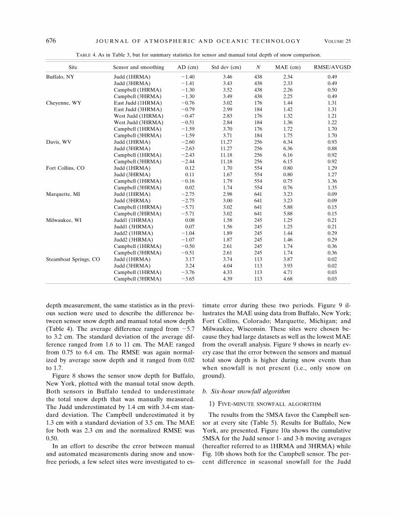
depth measurement, the same statistics as in the previ-ous section were used to describe the difference be-tween sensor snow depth and manual total snow depth(Table 4). The average difference ranged from �5.7to 3.2 cm. The standard deviation of the average dif-ference ranged from 1.6 to 11 cm. The MAE rangedfrom 0.75 to 6.4 cm. The RMSE was again normal-ized by average snow depth and it ranged from 0.02to 1.7.

Figure 8 shows the sensor snow depth for Buffalo,New York, plotted with the manual total snow depth.Both sensors in Buffalo tended to underestimatethe total snow depth that was manually measured.The Judd underestimated by 1.4 cm with 3.4-cm stan-dard deviation. The Campbell underestimated it by1.3 cm with a standard deviation of 3.5 cm. The MAEfor both was 2.3 cm and the normalized RMSE was0.50.

In an effort to describe the error between manualand automated measurements during snow and snow-free periods, a few select sites were investigated to es-

timate error during these two periods. Figure 9 il-lustrates the MAE using data from Buffalo, New York;Fort Collins, Colorado; Marquette, Michigan; andMilwaukee, Wisconsin. These sites were chosen be-cause they had large datasets as well as the lowest MAEfrom the overall analysis. Figure 9 shows in nearly ev-ery case that the error between the sensors and manualtotal snow depth is higher during snow events thanwhen snowfall is not present (i.e., only snow onground).

b. Six-hour snowfall algorithm

1) FIVE-MINUTE SNOWFALL ALGORITHM

The results from the 5MSA favor the Campbell sen-sor at every site (Table 5). Results for Buffalo, NewYork, are presented. Figure 10a shows the cumulative5MSA for the Judd sensor 1- and 3-h moving averages(hereafter referred to as 1HRMA and 3HRMA) whileFig. 10b shows both for the Campbell sensor. The per-cent difference in seasonal snowfall for the Judd

TABLE 4. As in Table 3, but for summary statistics for sensor and manual total depth of snow comparison.

Site Sensor and smoothing AD (cm) Std dev (cm) N MAE (cm) RMSE/AVGSD

Buffalo, NY Judd (1HRMA) �1.40 3.46 438 2.34 0.49Judd (3HRMA) �1.41 3.43 438 2.33 0.49Campbell (1HRMA) �1.30 3.52 438 2.26 0.50Campbell (3HRMA) �1.30 3.49 438 2.25 0.49

Cheyenne, WY East Judd (1HRMA) �0.76 3.02 176 1.44 1.31East Judd (3HRMA) �0.79 2.99 184 1.42 1.31West Judd (1HRMA) �0.47 2.83 176 1.32 1.21West Judd (3HRMA) �0.51 2.84 184 1.36 1.22Campbell (1HRMA) �1.59 3.70 176 1.72 1.70Campbell (3HRMA) �1.59 3.71 184 1.75 1.70

Davis, WV Judd (1HRMA) �2.60 11.27 256 6.34 0.93Judd (3HRMA) �2.63 11.27 256 6.36 0.88Campbell (1HRMA) �2.43 11.18 256 6.16 0.92Campbell (3HRMA) �2.44 11.18 256 6.15 0.92

Fort Collins, CO Judd (1HRMA) 0.12 1.70 554 0.80 1.29Judd (3HRMA) 0.11 1.67 554 0.80 1.27Campbell (1HRMA) �0.16 1.79 554 0.75 1.36Campbell (3HRMA) 0.02 1.74 554 0.76 1.35

Marquette, MI Judd (1HRMA) �2.75 2.98 641 3.23 0.09Judd (3HRMA) �2.75 3.00 641 3.23 0.09Campbell (1HRMA) �5.71 3.02 641 5.88 0.15Campbell (3HRMA) �5.71 3.02 641 5.88 0.15

Milwaukee, WI Judd1 (1HRMA) 0.08 1.58 245 1.25 0.21Judd1 (3HRMA) 0.07 1.56 245 1.25 0.21Judd2 (1HRMA) �1.04 1.89 245 1.44 0.29Judd2 (3HRMA) �1.07 1.87 245 1.46 0.29Campbell (1HRMA) �0.50 2.61 245 1.74 0.36Campbell (3HRMA) �0.51 2.61 245 1.74 0.36

Steamboat Springs, CO Judd (1HRMA) 3.17 3.74 113 3.87 0.02Judd (3HRMA) 3.24 4.04 113 3.93 0.02Campbell (1HRMA) �3.76 4.33 113 4.71 0.03Campbell (3HRMA) �3.65 4.39 113 4.68 0.03


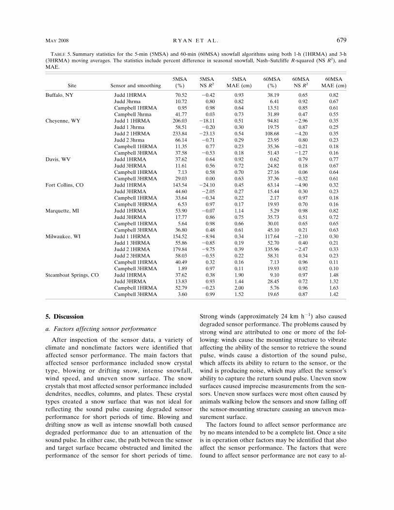
1HRMA and 3HRMA was 70.5% and 10.7%, respec-tively (Table 5). The percent difference for both theCampbell 1HRMA and 3HRMA was 0.95% and41.8%, respectively (Table 5). The Nash–Sutcliffe R-squared for the Judd 1HRMA and 3HRMA was �0.42and 0.80, respectively (Table 5). For the Campbell1HRMA and 3HRMA, the Nash–Sutcliffe R-squaredwas 0.98 and 0.03, respectively (Table 5). The MAE inthe incremental snowfall measurements for the Judd1HRMA and 3HRMA was 0.93 and 0.82 cm, respec-tively (Table 5). The MAE for the Campbell 1HRMAand 3HRMA was 0.64 and 0.73 cm, respectively (Table

5). The Campbell 1HRMA did the best at predicting6-h snowfall for Buffalo using this method. The Camp-bell 1HRMA had the highest Nash–Sutcliffe R-squaredas well as the lowest percent difference in seasonal totalsnowfall and MAE.

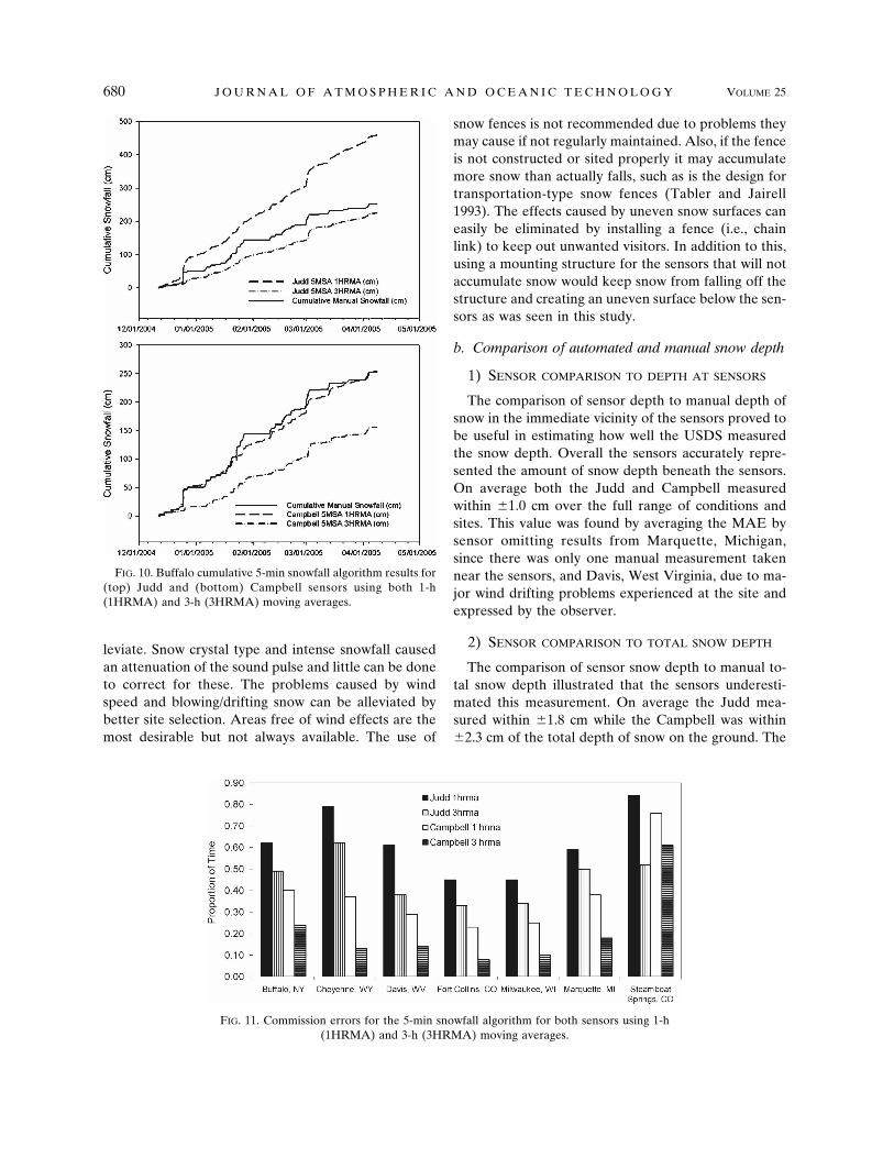
The CEs are shown in Fig. 11. The Campbell3HRMA consistently had the lowest CE, followed bythe Campbell 1HRMA, then the Judd 3HRMA andfinally the Judd 1HRMA. The minimum CE wasachieved by the Campbell 1HRMA in Fort Collins,Colorado. The maximum CE was achieved by the Judd1HRMA in Steamboat Springs, Colorado.

FIG. 8. Buffalo total snow depth plotted with automated data for the (top) Judd and(bottom) Campbell sensors for the snow season 2004/05.

MAY 2008 R Y A N E T A L . 677


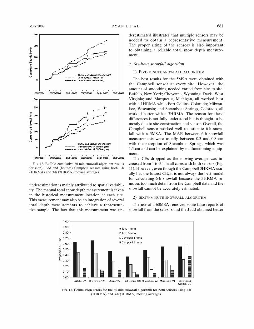
The results of the 60MSA differ by site and are notas consistent as the 5MSA (Table 5). At some sitesthe results favor the Judd and at others they favorthe Campbell. For Buffalo, New York, the cumula-tive seasonal snowfall for the Judd 1HRMA and3HRMA is shown in Fig. 12a while the Campbellis shown in Fig. 12b. The percent difference in seasonalsnowfall for the Judd 1HRMA and 3HRMA was38.2% and 6.4%, respectively (Table 5). The per-cent difference for the Campbell 1HRMA and3HRMA was 13.5% and 31.9%, respectively (Table 5).The Nash–Sutcliffe for the Judd 1HRMA and 3HRMAwas 0.65 and 0.92, respectively, while the Campbell1HRMA and 3HRMA was 0.85 and 0.47, respectively(Table 5). The MAE for the Judd 1HRMA and3HRMA was 0.82 and 0.67 cm, respectively, whilethe Campbell was 0.61 cm for the 1HRMA and 0.55 cmfor the 3HRMA (Table 5). In this case the Judd3HRMA did the best at predicting the 6-h snowfall for

Buffalo with the largest Nash–Sutcliffe R-squared andthe lowest percent difference in seasonal snowfall. TheMAE was similar for each method and sensor (Ta-ble 5).

Again, the CEs were calculated for the 60MSA (Fig.13). The results are similar to the 5MSA. The Campbell3HRMA consistently had the lowest CE (with the ex-ception of Steamboat Springs, Colorado), followed bythe Campbell 1HRMA, then the Judd 3HRMA, andfinally the Judd 1HRMA. The minimum CE wasachieved with the Campbell 3HRMA in Fort Collins,Colorado. The maximum CE was achieved by the Judd1HRMA in Cheyenne, Wyoming.

The errors of omission for the Judd and Campbellsensors are shown in Figs. 14a and 14b. The omissionerrors depict the proportion of time the manual datameasured snow and the sensors did not. At most sitesthe omission errors increased from the 5MSA to the60MSA. This illustrates that the 60MSA is omittingsnowfall events by taking the difference in snow depthover the longer time period.

FIG. 9. Comparison of MAE between automated and manual total snow depth during periods where snowfall is present andsnowfall is not.


5. Discussion

a. Factors affecting sensor performance

After inspection of the sensor data, a variety ofclimate and nonclimate factors were identified thataffected sensor performance. The main factors thataffected sensor performance included snow crystaltype, blowing or drifting snow, intense snowfall,wind speed, and uneven snow surface. The snowcrystals that most affected sensor performance includeddendrites, needles, columns, and plates. These crystaltypes created a snow surface that was not ideal forreflecting the sound pulse causing degraded sensorperformance for short periods of time. Blowing anddrifting snow as well as intense snowfall both causeddegraded performance due to an attenuation of thesound pulse. In either case, the path between the sensorand target surface became obstructed and limited theperformance of the sensor for short periods of time.

Strong winds (approximately 24 km h�1) also causeddegraded sensor performance. The problems caused bystrong wind are attributed to one or more of the fol-lowing: winds cause the mounting structure to vibrateaffecting the ability of the sensor to retrieve the soundpulse, winds cause a distortion of the sound pulse,which affects its ability to return to the sensor, or thewind is producing noise, which may affect the sensor’sability to capture the return sound pulse. Uneven snowsurfaces caused imprecise measurements from the sen-sors. Uneven snow surfaces were most often caused byanimals walking below the sensors and snow falling offthe sensor-mounting structure causing an uneven mea-surement surface.

The factors found to affect sensor performance areby no means intended to be a complete list. Once a siteis in operation other factors may be identified that alsoaffect the sensor performance. The factors that werefound to affect sensor performance are not easy to al-

TABLE 5. Summary statistics for the 5-min (5MSA) and 60-min (60MSA) snowfall algorithms using both 1-h (1HRMA) and 3-h(3HRMA) moving averages. The statistics include percent difference in seasonal snowfall, Nash–Sutcliffe R-squared (NS R2), andMAE.

Site Sensor and smoothing5MSA

(%)5MSANS R2

5MSAMAE (cm)

60MSA(%)

60MSANS R2

60MSAMAE (cm)

Buffalo, NY Judd 1HRMA 70.52 �0.42 0.93 38.19 0.65 0.82Judd 3hrma 10.72 0.80 0.82 6.41 0.92 0.67Campbell 1HRMA 0.95 0.98 0.64 13.51 0.85 0.61Campbell 3hrma 41.77 0.03 0.73 31.89 0.47 0.55

Cheyenne, WY Judd 1 1HRMA 206.03 �18.11 0.51 94.81 �2.96 0.35Judd 1 3hrma 58.51 �0.20 0.30 19.75 0.87 0.25Judd 2 1HRMA 233.84 �23.13 0.54 108.68 �4.20 0.35Judd 2 3hrma 66.14 �0.71 0.29 23.95 0.80 0.23Campbell 1HRMA 11.35 0.77 0.23 35.36 �0.21 0.18Campbell 3HRMA 37.58 �0.53 0.18 51.43 �1.27 0.16

Davis, WV Judd 1HRMA 37.62 0.64 0.92 0.62 0.79 0.77Judd 3HRMA 11.61 0.56 0.72 24.82 0.18 0.67Campbell 1HRMA 7.13 0.58 0.70 27.16 0.06 0.64Campbell 3HRMA 29.03 0.00 0.63 37.36 �0.32 0.61

Fort Collins, CO Judd 1HRMA 143.54 �24.10 0.45 63.14 �4.90 0.32Judd 3HRMA 44.60 �2.05 0.27 15.44 0.30 0.23Campbell 1HRMA 33.64 �0.34 0.22 2.17 0.97 0.18Campbell 3HRMA 6.53 0.97 0.17 19.93 0.70 0.16

Marquette, MI Judd 1HRMA 53.90 �0.07 1.14 5.29 0.98 0.82Judd 3HRMA 17.77 0.86 0.75 35.73 0.51 0.72Campbell 1HRMA 5.64 0.98 0.66 30.01 0.65 0.65Campbell 3HRMA 36.80 0.48 0.61 45.10 0.21 0.63

Milwaukee, WI Judd 1 1HRMA 154.52 �8.94 0.34 117.64 �2.10 0.30Judd 1 3HRMA 55.86 �0.85 0.19 52.70 0.40 0.21Judd 2 1HRMA 179.84 �9.75 0.39 135.96 �2.47 0.33Judd 2 3HRMA 58.03 �0.55 0.22 58.31 0.34 0.23Campbell 1HRMA 40.49 0.32 0.16 7.13 0.96 0.11Campbell 3HRMA 1.89 0.97 0.11 19.93 0.92 0.10

Steamboat Springs, CO Judd 1HRMA 37.62 0.38 1.90 9.10 0.97 1.48Judd 3HRMA 13.83 0.93 1.44 28.45 0.72 1.32Campbell 1HRMA 52.79 �0.23 2.00 5.76 0.96 1.63Campbell 3HRMA 3.60 0.99 1.52 19.65 0.87 1.42

MAY 2008 R Y A N E T A L . 679

leviate. Snow crystal type and intense snowfall causedan attenuation of the sound pulse and little can be doneto correct for these. The problems caused by windspeed and blowing/drifting snow can be alleviated bybetter site selection. Areas free of wind effects are themost desirable but not always available. The use of

snow fences is not recommended due to problems theymay cause if not regularly maintained. Also, if the fenceis not constructed or sited properly it may accumulatemore snow than actually falls, such as is the design fortransportation-type snow fences (Tabler and Jairell1993). The effects caused by uneven snow surfaces caneasily be eliminated by installing a fence (i.e., chainlink) to keep out unwanted visitors. In addition to this,using a mounting structure for the sensors that will notaccumulate snow would keep snow from falling off thestructure and creating an uneven surface below the sen-sors as was seen in this study.

b. Comparison of automated and manual snow depth

1) SENSOR COMPARISON TO DEPTH AT SENSORS

The comparison of sensor depth to manual depth ofsnow in the immediate vicinity of the sensors proved tobe useful in estimating how well the USDS measuredthe snow depth. Overall the sensors accurately repre-sented the amount of snow depth beneath the sensors.On average both the Judd and Campbell measuredwithin �1.0 cm over the full range of conditions andsites. This value was found by averaging the MAE bysensor omitting results from Marquette, Michigan,since there was only one manual measurement takennear the sensors, and Davis, West Virginia, due to ma-jor wind drifting problems experienced at the site andexpressed by the observer.

2) SENSOR COMPARISON TO TOTAL SNOW DEPTH

The comparison of sensor snow depth to manual to-tal snow depth illustrated that the sensors underesti-mated this measurement. On average the Judd mea-sured within �1.8 cm while the Campbell was within�2.3 cm of the total depth of snow on the ground. The

FIG. 11. Commission errors for the 5-min snowfall algorithm for both sensors using 1-h(1HRMA) and 3-h (3HRMA) moving averages.

FIG. 10. Buffalo cumulative 5-min snowfall algorithm results for(top) Judd and (bottom) Campbell sensors using both 1-h(1HRMA) and 3-h (3HRMA) moving averages.


underestimation is mainly attributed to spatial variabil-ity. The manual total snow depth measurement is takenin the historical measurement location at each site.This measurement may also be an integration of severaltotal depth measurements to achieve a representa-tive sample. The fact that this measurement was un-

derestimated illustrates that multiple sensors may beneeded to obtain a representative measurement.The proper siting of the sensors is also importantto obtaining a reliable total snow depth measure-ment.

c. Six-hour snowfall algorithm

1) FIVE-MINUTE SNOWFALL ALGORITHM

The best results for the 5MSA were obtained withthe Campbell sensor at every site. However, theamount of smoothing needed varied from site to site.Buffalo, New York; Cheyenne, Wyoming; Davis, WestVirginia; and Marquette, Michigan, all worked bestwith a 1HRMA while Fort Collins, Colorado; Milwau-kee, Wisconsin; and Steamboat Springs, Colorado, allworked better with a 3HRMA. The reason for thesedifferences is not fully understood but is thought to bemostly due to site construction and sensor. Overall, theCampbell sensor worked well to estimate 6-h snow-fall with a 5MSA. The MAE between 6-h snowfallmeasurements were usually between 0.3 and 0.8 cmwith the exception of Steamboat Springs, which was1.5 cm and can be explained by malfunctioning equip-ment.

The CEs dropped as the moving average was in-creased from 1 to 3 h in all cases with both sensors (Fig.11). However, even though the Campbell 3HRMA usu-ally has the lowest CE, it is not always the best modelfor calculating 6-h snowfall because the 3HRMA re-moves too much detail from the Campbell data and thesnowfall cannot be accurately estimated.


The use of a 60MSA removed some false reports ofsnowfall from the sensors and the Judd obtained better

FIG. 12. Buffalo cumulative 60-min snowfall algorithm resultsfor (top) Judd and (bottom) Campbell sensors using both 1-h(1HRMA) and 3-h (3HRMA) moving averages.

FIG. 13. Commission errors for the 60-min snowfall algorithm for both sensors using 1-h(1HRMA) and 3-h (3HRMA) moving averages.

MAY 2008 R Y A N E T A L . 681

results than with the 5MSA. However, taking thechange over the longer 60-min period may omit smallevents that occurred over that time interval and wouldnot accurately depict the actual snowfall at a site wherethis algorithm is used. The omission errors illustratedthis point (Figs. 14a,b).

The reasons for the differences in algorithm perfor-mance between sites are highly speculative and wereattributed to both siting and sensors. Poor siting andinstallation can add more variation into the data, whichwould need more smoothing. The sensor resolution in-troduces problems into calculating snowfall. TheCampbell sensor has a finer data resolution that doesnot produce as many false snowfall reports as the Judd.The errors of commission illustrate this point. The60MSA CEs (Fig. 13) illustrated that the Judd sensorhas a coarser data resolution that allows it to appear toaccumulate snow even under snow-free conditions. Thepatterns are consistent with the 5MSA; as the amountof smoothing increases the CEs decrease.

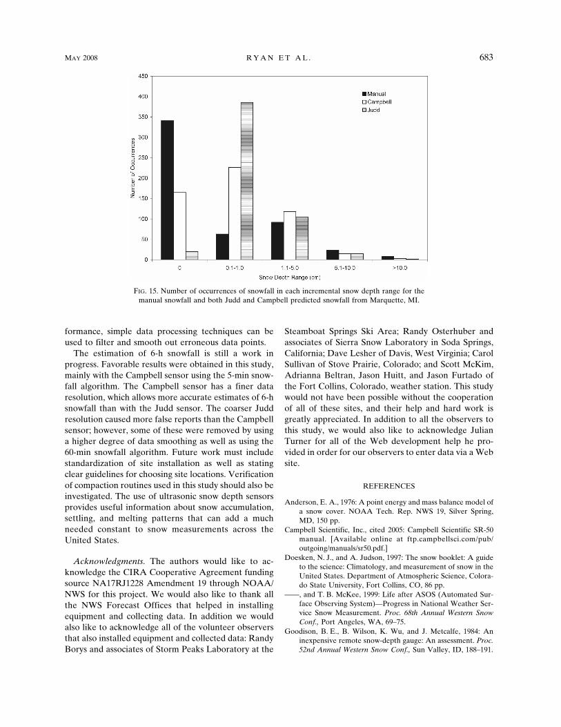
The CEs suggest that the sensors are not measuring“no snow” very well. Figure 15 shows the number ofoccurrences for each range of snowfall that was re-ported manually as well as being estimated by the sen-

sors for Marquette, Michigan, using the statistically bestmodel for each sensor. The sensors did not reportnearly as many zero snow depths as were manuallymeasured, and they also overestimated the number ofoccurrences that fell in the 0.1–1.0-cm range. This isagain due to sensor resolution, which caused the sen-sors to measure snow when there was none manuallyreported. The reports that were supposed to be placedin the zero range for the sensors actually fell in the0.1–1.0-cm range.

6. Conclusions

This evaluation of ultrasonic snow depth sensors hasshown promising results that these sensors can be usedto restore snow measurements at hundreds of auto-mated sites across the United States and add more ob-jectivity to a measurement often known to be subjec-tive. Even though both sensors did accurately measurethe snow depth below them, the underestimation of thetotal snow depth measurement illustrates the need forproper siting as well as the need for multiple sensors toobtain a representative measurement. Even thoughseveral factors were identified that affected sensor per-

FIG. 14. Omission errors for (top) Judd and (bottom) Campbell algorithms (both 5- and60-min algorithms using 1- and 3-h moving averages) by site.


formance, simple data processing techniques can beused to filter and smooth out erroneous data points.

The estimation of 6-h snowfall is still a work inprogress. Favorable results were obtained in this study,mainly with the Campbell sensor using the 5-min snow-fall algorithm. The Campbell sensor has a finer dataresolution, which allows more accurate estimates of 6-hsnowfall than with the Judd sensor. The coarser Juddresolution caused more false reports than the Campbellsensor; however, some of these were removed by usinga higher degree of data smoothing as well as using the60-min snowfall algorithm. Future work must includestandardization of site installation as well as statingclear guidelines for choosing site locations. Verificationof compaction routines used in this study should also beinvestigated. The use of ultrasonic snow depth sensorsprovides useful information about snow accumulation,settling, and melting patterns that can add a muchneeded constant to snow measurements across theUnited States.

Acknowledgments. The authors would like to ac-knowledge the CIRA Cooperative Agreement fundingsource NA17RJ1228 Amendment 19 through NOAA/NWS for this project. We would also like to thank allthe NWS Forecast Offices that helped in installingequipment and collecting data. In addition we wouldalso like to acknowledge all of the volunteer observersthat also installed equipment and collected data: RandyBorys and associates of Storm Peaks Laboratory at the

Steamboat Springs Ski Area; Randy Osterhuber andassociates of Sierra Snow Laboratory in Soda Springs,California; Dave Lesher of Davis, West Virginia; CarolSullivan of Stove Prairie, Colorado; and Scott McKim,Adrianna Beltran, Jason Huitt, and Jason Furtado ofthe Fort Collins, Colorado, weather station. This studywould not have been possible without the cooperationof all of these sites, and their help and hard work isgreatly appreciated. In addition to all the observers tothis study, we would also like to acknowledge JulianTurner for all of the Web development help he pro-vided in order for our observers to enter data via a Website.

REFERENCES

Anderson, E. A., 1976: A point energy and mass balance model ofa snow cover. NOAA Tech. Rep. NWS 19, Silver Spring,MD, 150 pp.

Campbell Scientific, Inc., cited 2005: Campbell Scientific SR-50manual. [Available online at ftp.campbellsci.com/pub/outgoing/manuals/sr50.pdf.]

Doesken, N. J., and A. Judson, 1997: The snow booklet: A guideto the science: Climatology, and measurement of snow in theUnited States. Department of Atmospheric Science, Colora-do State University, Fort Collins, CO, 86 pp.

——, and T. B. McKee, 1999: Life after ASOS (Automated Sur-face Observing System)—Progress in National Weather Ser-vice Snow Measurement. Proc. 68th Annual Western SnowConf., Port Angeles, WA, 69–75.

Goodison, B. E., B. Wilson, K. Wu, and J. Metcalfe, 1984: Aninexpensive remote snow-depth gauge: An assessment. Proc.52nd Annual Western Snow Conf., Sun Valley, ID, 188–191.

FIG. 15. Number of occurrences of snowfall in each incremental snow depth range for themanual snowfall and both Judd and Campbell predicted snowfall from Marquette, MI.

MAY 2008 R Y A N E T A L . 683

——, J. R. Metcalfe, R. A. Wilson, and K. Jones, 1988: The Ca-nadian automatic snow depth sensor: A performance update.Proc. 56th Annual Western Snow Conf., Kalispell, MT, 178–181.

Jordan, R., 1991: A one-dimensional temperature model for asnow cover: Technical Documentation for SNTHERM.89.Special Rep. 91-16, Cold Regions Research and EngineeringLaboratory, U.S. Army Corps of Engineers, 64 pp.

Judd, D., cited 2005: Judd Communications online manual.[Available online at www.juddcom.com/ds2manual.pdf.]

Kunkel, K. E., M. Palecki, K. G. Hubbard, D. Robinson, K. Red-mond, and D. Easterling, 2007: Trend identification in 20thcentury U.S. snowfall: The challenges. J. Atmos. OceanicTechnol., 24, 64–73.

Lea, J., and J. Lea, 1998: Snowpack depth and density changesduring rain on snow events at Mt. Hood Oregon. Interna-tional Conf. on Snow Hydrology: The Integration of Physical,Chemical and Biological Systems, CRREL Special Rep. 981-10, Brownsville, VT, 46 pp.

McKee, T. B., N. J. Doesken, C. A. Davey, and R. A. Pielke Sr.,2000: Climate data continuity with ASOS: Report for periodApril 1996 through June 2000. Climatology Rep. 00-3, De-partment of Atmospheric Science, Colorado State Univer-sity, Fort Collins, CO, 82 pp.

Nash, J. E., and J. V. Sutcliffe, 1970: River flow forecastingthrough conceptual models, part 1—A discussion of prin-ciples. J. Hydrol., 10, 282–290.

NRC, 1998: Future of the National Weather Service CooperativeObserver Network. National Research Council, NationalWeather Service Modernization Committee, National Acad-emy Press, Washington, DC, 78 pp.

NWS, cited 1996: Snow measurement guidelines (revised 10/28/96). NOAA/NWS, Silver Spring, MD. [Available online athttp://www.noaa.gov/os/coop/snowguid.htm.]

——, 2004: Automated Surface Observing System (ASOS). Re-lease Note on All-Weather Precipitation Gage, 36 pp. [Avail-able online at http://www.nws.noaa.gov/ops2/Surface/documents/awpag27B6relnotes.pdf.]

——, cited 2006: 8 inch non-recording standard rain gage. Na-tional Weather Service–National Training Center. [Availableonline at http://www.nwstc.noaa.gov/METEOR/srg/rain8in.html.]

Robinson, D. A., 1989: Evaluation of the collection, archiving,and publication of daily snow data in the United States. Phys.Geogr., 10, 120–130.

Tabler, R. D., and R. L. Jairell, 1993: Trapping efficiency of snowfences and implications for system design. Transport. Res.Record, 1387, 108–114.


Documents

Evaluation of Ultrasonic Snow Depth Sensors for U.S. Snow ...ccc.atmos.colostate.edu/pdfs/...etal-evaluating_snow_depth_sensors.pdf · Evaluation of Ultrasonic Snow Depth Sensors