1007

Journal of Oceanography, Vol. 60, pp. 1007 to 1021, 2004

Keywords:⋅⋅⋅⋅⋅ MODAS,⋅⋅⋅⋅⋅ data assimilation,⋅⋅⋅⋅⋅ South China SeaMonsoon Experi-ment,

⋅⋅⋅⋅⋅ thermocline,⋅⋅⋅⋅⋅ halocline,⋅⋅⋅⋅⋅ skill score,⋅⋅⋅⋅⋅ bias,⋅⋅⋅⋅⋅ root-mean squareerror.

* Corresponding author. E-mail: pcchu@nps.navy.mil

Copyright © The Oceanographic Society of Japan.

Evaluation of the U.S. Navy’s Modular Ocean DataAssimilation System (MODAS) Using South ChinaSea Monsoon Experiment (SCSMEX) Data

PETER C. CHU*, WANG GUIHUA and CHENWU FAN

Naval Ocean Analysis and Prediction Laboratory, Department of Oceanography,Naval Postgraduate School, Monterey, CA 93943, U.S.A.

(Received 1 September 2003; in revised form 10 March 2004; accepted 15 March 2004)

The Navy’s Modular Ocean Data Assimilation System (MODAS) is an oceanographictool to create high-resolution temperature and salinity on three-dimensional grids,by assimilating a wide range of ocean observations into a starting field. The MODASproducts are used to generate the sound speed for ocean acoustic modeling applica-tions. Hydrographic data acquired from the South China Sea Monsoon Experiment(SCSMEX) from April through June 1998 are used to verify the MODAS model.MODAS has the capability to provide reasonably good temperature and salinitynowcast fields. The errors have a Gaussian-type distribution with mean temperaturenearly zero and mean salinity of –0.2 ppt. The standard deviations of temperatureand salinity errors are 0.98°C and 0.22 ppt, respectively. The skill score of the tem-perature nowcast is positive, except at depth between 1750 and 2250 m. The skillscore of the salinity nowcast is less than that of the temperature nowcast, especially atdepth between 300 and 400, where the skill score is negative. Thermocline and haloclineidentified from the MODAS temperature and salinity fields are weaker than thosebased on SCSMEX data. The maximum discrepancy between the two is in thethermocline and halocline. The thermocline depth estimated from the MODAS tem-perature field is 10–40 m shallower than that from the SCSMEX data. The verticaltemperature gradient across the thermocline computed from the MODAS field isaround 0.14°C/m, weaker than that calculated from the SCSMEX data (0.19°–0.27°C/m). The thermocline thickness computed from the MODAS field has less temporalvariation than that calculated from the SCSMEX data (40–100 m). The halocline depthestimated from the MODAS salinity field is always deeper than that from the SCSMEXdata. Its thickness computed from the MODAS field varies slowly around 30 m, whichis generally thinner than that calculated from the SCSMEX data (28–46 m).

porated into a three-dimensional, gridded output field oftemperature and salinity. The MODAS-2.1 products areused to generate the sound speed field for ocean acousticmodeling applications. Other derived fields, which maybe generated and examined by the user, include such two-dimensional and three-dimensional quantities as verticalshear of geostrophic current, mixed layer depth, soniclayer depth, deep sound channel axis depth, depth excess,and critical depth. These are employed in a wide varietyof naval applications.

The first generation of this system, MODAS-1.0, wasinitially designed in the early 1990’s to perform deep-water analyses that produced outputs that supported deep-water anti-submarine warfare operations. However,MODAS-1.0 was constrained at depths greater than 100

1. IntroductionAn advanced version of the Navy’s Modular Ocean

Data Assimilation System (MODAS-2.1), developed atthe Naval Research Laboratory, is in operational use atthe Naval Oceanographic Office to provide twice-daily,three-dimensional temperature and salinity fields. Thedata can be downloaded from the website: http://www.navo.navy.mil. Its data assimilation capabilities maybe applied to a wide range of input data, including ir-regularly located in-situ sampling, satellite, andclimatological data. Available measurements are incor-

Evaluation of the U.S. Navy’s MODAS Model 1011

location then the deviation at each depth is estimated.Adding these estimated deviations to the climatology pro-duces the synthetic profiles.

4.4 MODAS special treatmentsTwo treatments distinguish MODAS from ordinary

optimum interpolation schemes: (1) “synthetic” tempera-ture profiles generated using surface height and tempera-ture, and (2) salinity as a function of temperature. TheMODAS first treatment is to establish linear regressionrelationships between (SST, SSH) with temperature at agiven depth. Synthetic temperature profiles extending toa maximum depth of 1500 m are computed from theseregression relationships. The MODAS second treatmentis to determine the relationship between salinity and tem-perature at each position, depth, and time of year, by lo-cally weighted linear regression from the subset of ob-servations having both temperature and salinity (Fox etal., 2002).

5. Methodology of VerificationObservational and climatological data are needed for

MODAS verification. Both MODAS and climatologicaldata are compared with the observational data. Observa-tional data are used for determining error statistics.Climatological data are used to verify the added value ofthe MODAS model. The MODAS has added value if thedifference between MODAS and observational data is lessthan the difference between climatological and observa-tional data. MODAS, climatological, and SCSMEX dataψ (temperature, salinity) are represented by ψm, ψc, andψo.

5.1 Climatological dataAn independent climatological dataset should be used

as reference to verify MODAS. Since the World OceanAtlas (WOA) 1994 (Levitus and Boyer, 1994a, b) is usedto build MODAS climatology (Fox et al., 2002), the Na-vy’s GDEM climatological monthly mean temperature andsalinity dataset with 1/2° resolution is taken as the refer-ence. Observational data for building the current versionof GDEM climatology were obtained from the Navy’sMaster Oceanographic Observational Data Set (MOODS),which contains records of more than 6 million tempera-ture and 1.2 million salinity profiles since early last cen-tury. The GDEM data can be obtained from the website:http://www.navo.navy.mil.

The basic design concept of GDEM is the determi-nation of a set of analytical curves that represent the meanvertical distributions of temperature and salinity for gridcells through the averaging of the coefficients of the math-ematical expressions for the curves found for individualprofiles (Teague et al., 1990). Different families of rep-resentative curves have been chosen for shallow, mid-

depth, and deep ranges, each chosen so that the numberof parameters required to yield a smooth, mean profileover the range was minimized. The monthly mean three-dimensional temperature and salinity fields obtained fromthe GDEM dataset is similar to the climatological monthlymean fields computed directly from the MOODS, as de-picted in Chu et al. (1999b).

5.2 Error statisticsIf the observational data are located at (xi, yj, z, t),

we interpolate the MODAS and GDEM data into the ob-servational points and form modeled and climatologicaldata sets. The difference in ψ between modeled and ob-served values

∆m i j m i j o i jx y z t x y z t x y z tψ ψ ψ, , , , , , , , , ,( ) = ( ) − ( ) ( )1

represents the model error. The difference in ψ betweenclimatological and observed values

∆c i j c i j o i jx y z t x y z t x y z tψ ψ ψ, , , , , , , , , ,( ) = ( ) − ( ) ( )2

represents the prediction error using the climatologicalvalues. We may take the probability histogram of ∆ψ asthe error distribution.

The bias, mean-square-error (MSE), and root-mean-square error (RMSE) for the MODAS model

BIAS

MSE

RMSE MSE

m oN

x y z t

m oN

x y z t

m o m o

m i jji

m i jji

, , , , ,

, , , , ,

, , ,

( ) = ( )

( ) = ( )[ ]( ) = ( ) ( )

∑∑

∑∑

1

1

3

2

∆

∆

ψ

ψ

and for the reference model (e.g., climatology),

BIAS

MSE

RMSE MSE

c oN

x y z t

c oN

x y z t

c o c o

c i jji

c i jji

, , , , ,

, , , , ,

, , ,

( ) = ( )

( ) = ( )[ ]( ) = ( ) ( )

∑∑

∑∑

1

1

4

2

∆

∆

ψ

ψ

are commonly used for evaluation of the model perform-ance. Here N is the total number of horizontal points.

5.3 MODAS skill scoreMODAS accuracy is usually defined as the average

1008 P. C. Chu et al.

m because it used climatological data from the originalGeneralized Digital Environmental Model (GDEM) es-tablished from the Master Observational OceanographicData Set (MOODS). The capabilities of MODAS-1.0 wereincreased when GDEM was initially augmented with ashallow water database (SWDB), but at the time, SWDBwas limited to the northern hemisphere. The NOAA glo-bal database, which has less horizontal resolution thanGDEM, was used as a second source for the first guessfield in MODAS-1.0. In addition, in MODAS-1.0 someof the algorithms for processing and for performing in-terpolations were designed for speed and efficiency indeep waters, at the cost of making some assumptions aboutthe topography. This shortcut method extended all obser-vational profiles to a common depth, even if the depthwas well below the ocean bottom depth, by splicing ontoclimatology. The error introduced using this shortcutmethod is amplified when this method is applied to shal-low water regions.

The second generation, MODAS-2.1, was created toovercome the limitations of MODAS-1.0. One of themajor implementations was the development of MODASinternal ocean climatology (Static MODAS climatology)for both deep and shallow depths. Static MODAS clima-tology is produced using the historical T, S profile data,i.e., the MOODS. Static MODAS climatology covers theocean globally to a minimum depth of 5 meters and hasvariable horizontal resolution from 7.5 minutes to 60minutes. The static MODAS climatology also containsimportant statistical descriptors required for optimumanalysis of observations that include bi-monthly meansof temperature, coefficients for calculation of salinityfrom temperature, standard deviations of temperature andsalinity, and coefficients for several models relating tem-perature and mixed layer depth to surface temperature andsteric height anomaly. MODAS-2.1 performs separateoptimum interpolation analysis for each depth above theocean bottom.

The Naval Oceanographic Office (1999) conductedan operational test of MODAS 2.1 using temperature ob-servations from April 15 to May 14, 1999 for six areas:Kamchatka Sea (13 profiles), Bay of Biscay (58 profiles),Greenland-Icelandic-Norwegian (GIN) Sea (120 profiles),Northwest Atlantic (profiles: 133), and Northeast Pacific(profiles: 166), and Japan Sea (profiles: 692). The root-mean-square (rms) errors between MODAS products andobservations were usually smaller than that between theclimatology (i.e., GDEM) and observations. Another en-couraging fact is the small rms errors occurring in theJapan Sea, the Northwest Atlantic, and the GIN Sea area—all have high spatial variability. MODAS 2.1 thus dis-plays improved capability over a GDEM-based MODASanalysis in fairly complex ocean regimes. However, thetest was only on the comparison of temperature fields.

No evaluation was given of the MODAS salinity field.Furthermore, the MODAS capability for nowcastingthermocline/halocline has not been evaluated.

A recent development is to use the MODAS tempera-ture and salinity fields to initialize an ocean predictionmodel such as the Princeton Ocean Model (Chu et al.,2001). There is thus an urgent need to evaluate theMODAS salinity field as well as the thermocline/haloclinestructures. The South China Sea Monsoon Experiment(SCSMEX) provides a unique opportunity for such anevaluation. The SCSMEX data have not been assimilatedinto MODAS. Hydrographic data acquired from SCSMEXfor April through June 1998 are used to verify MODAStemperature and salinity products.

2. South China SeaThe South China Sea (SCS) is a semi-enclosed tropi-

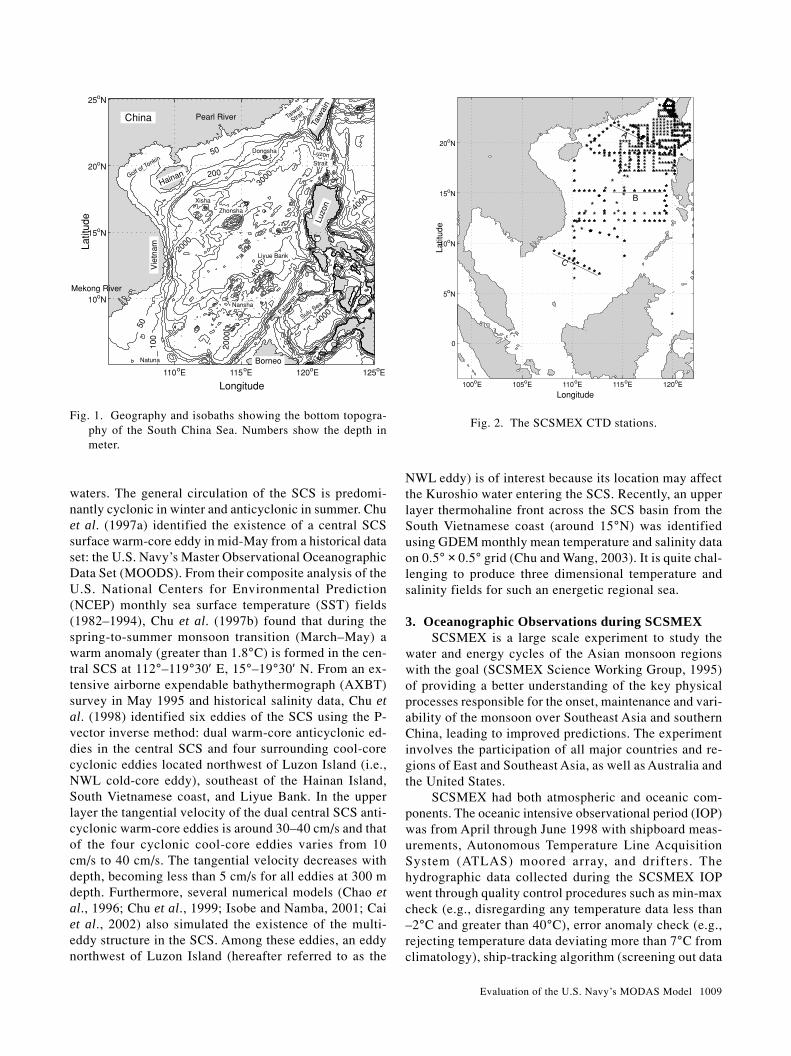
cal sea located between the Asian land mass to the northand west, the Philippine Islands to the east, Borneo to thesoutheast, and Indonesia to the south (Fig. 1), covering atotal area of 3.5 × 106 km2. It includes the shallow Gulfof Thailand and connections to the East China Sea(through Taiwan Strait), the Pacific Ocean (through LuzonStrait), Sulu Sea, Java Sea (through Gasper and KarimataStraits) and to the Indian Ocean (through the Strait ofMalacca). All of these straits are shallow except LuzonStrait, the maximum depth of which is 1800 m. The com-plex topography includes a broad, shallow shelf in thesouth/southwest; the continental shelf of the Asian land-mass in the north, extending from the Gulf of Tonkin toTaiwan Strait; a deep, elliptical shaped basin in the center,and numerous reef islands and underwater plateaus scat-tered throughout. The shelf that extends from the Gulf ofTonkin to the Taiwan Strait is consistently nearly 70 mdeep, averaging 150 km in width; the central deep basinis 1900 km along its major axis (northeast-southwest) andapproximately 1100 km along its minor axis, extendingto over 4000 m deep. The south/southwest SCS shelf isthe submerged connection between southeastern Asia,Malaysia, Sumatra, Java, and Borneo and reaches 100 mdepth in the middle; the center of the Gulf of Thailand isabout 70 m deep.

The SCS is subjected to a seasonal monsoon system.From April to August, the weaker southwesterly summermonsoon winds result in a monthly mean wind stress ofjust over 0.1 N/m2. From November to March, the strongernortheasterly winter monsoon winds correspond to amaximum monthly mean wind stress of nearly 0.3 N/m2.During monsoon transition, the winds and surface cur-rents are highly variable.

Many studies have shown that the SCS circulationhas a multi-eddy structure. A survey by Wyrtki (1961)revealed complex temporal and spatial features of thesurface currents in both the SCS and the surrounding

Evaluation of the U.S. Navy’s MODAS Model 1009

waters. The general circulation of the SCS is predomi-nantly cyclonic in winter and anticyclonic in summer. Chuet al. (1997a) identified the existence of a central SCSsurface warm-core eddy in mid-May from a historical dataset: the U.S. Navy’s Master Observational OceanographicData Set (MOODS). From their composite analysis of theU.S. National Centers for Environmental Prediction(NCEP) monthly sea surface temperature (SST) fields(1982–1994), Chu et al. (1997b) found that during thespring-to-summer monsoon transition (March–May) awarm anomaly (greater than 1.8°C) is formed in the cen-tral SCS at 112°–119°30′ E, 15°–19°30′ N. From an ex-tensive airborne expendable bathythermograph (AXBT)survey in May 1995 and historical salinity data, Chu etal. (1998) identified six eddies of the SCS using the P-vector inverse method: dual warm-core anticyclonic ed-dies in the central SCS and four surrounding cool-corecyclonic eddies located northwest of Luzon Island (i.e.,NWL cold-core eddy), southeast of the Hainan Island,South Vietnamese coast, and Liyue Bank. In the upperlayer the tangential velocity of the dual central SCS anti-cyclonic warm-core eddies is around 30–40 cm/s and thatof the four cyclonic cool-core eddies varies from 10cm/s to 40 cm/s. The tangential velocity decreases withdepth, becoming less than 5 cm/s for all eddies at 300 mdepth. Furthermore, several numerical models (Chao etal., 1996; Chu et al., 1999; Isobe and Namba, 2001; Caiet al., 2002) also simulated the existence of the multi-eddy structure in the SCS. Among these eddies, an eddynorthwest of Luzon Island (hereafter referred to as the

NWL eddy) is of interest because its location may affectthe Kuroshio water entering the SCS. Recently, an upperlayer thermohaline front across the SCS basin from theSouth Vietnamese coast (around 15°N) was identifiedusing GDEM monthly mean temperature and salinity dataon 0.5° × 0.5° grid (Chu and Wang, 2003). It is quite chal-lenging to produce three dimensional temperature andsalinity fields for such an energetic regional sea.

3. Oceanographic Observations during SCSMEXSCSMEX is a large scale experiment to study the

water and energy cycles of the Asian monsoon regionswith the goal (SCSMEX Science Working Group, 1995)of providing a better understanding of the key physicalprocesses responsible for the onset, maintenance and vari-ability of the monsoon over Southeast Asia and southernChina, leading to improved predictions. The experimentinvolves the participation of all major countries and re-gions of East and Southeast Asia, as well as Australia andthe United States.

SCSMEX had both atmospheric and oceanic com-ponents. The oceanic intensive observational period (IOP)was from April through June 1998 with shipboard meas-urements, Autonomous Temperature Line AcquisitionSystem (ATLAS) moored array, and drifters. Thehydrographic data collected during the SCSMEX IOPwent through quality control procedures such as min-maxcheck (e.g., disregarding any temperature data less than–2°C and greater than 40°C), error anomaly check (e.g.,rejecting temperature data deviating more than 7°C fromclimatology), ship-tracking algorithm (screening out data

Fig. 1. Geography and isobaths showing the bottom topogra-phy of the South China Sea. Numbers show the depth inmeter.

Fig. 2. The SCSMEX CTD stations.

110 E 115 E 120 E 125 E

10 N

15 N

20 N

25 N

Longitude

Latit

ude

50

20030

00

4000

2000

4000

4000

2000

50

100

Vie

tnam

Hainan

Taiw

ain

Luzo

n

Borneo

Taiwan

Strait

Palawan

LuzonStrait

Dongsha

Xisha

Zhonsha

Liyue Bank

Nansha

Natuna

Sulu Sea

Golf of Tonkin

China Pearl River

Mekong River

100 E 105 E 110 E 115 E 120 E

0

5 N

10 N

15 N

20 N

Longitude

Latit

ude

*

*

** *

***

**

*

**

****

**** *********

**

****

**

***

***

****

*

*

*****

**

***

**********

* * * ***

**********

* * *

**********

*

** ** ***

*****

**

*

*

******

* * * * * * *

***************

********

***

* * * * * *

***

***

*****

********

********

**************** **

******** *

*

************* **************

*****

************

****************

* ***** ******

****************

************

****

*********************

**

*********

**********

****** ***

*************************

**************

***************

*****************************

*********** *****************************************

************

*********

****

*

*********

********

****** **********

* *

***

*** * * * * *

**

** *******

****

*****

**************

**

************

*********

************

* * ****

****

* * * *

***

*****

*

* *

***

*** * * **

*

*********

**

***

*****

*****

*

* *****

*

******

******

* * **** ** ****************************

******

** A

B

C

1010 P. C. Chu et al.

with obvious ship position errors), max-number limit (lim-iting a maximum number of observations within a speci-fied and rarely exceeded space-time window), and buddycheck (rejecting contradicting data). The climatologicaldata used for quality control are depicted in Chu et al.(1997a, b). After the quality control, the SCSMEX ocea-nographic data set contains 1742 conductivity-tempera-ture-depth (CTD) and mooring stations (Fig. 2). The ma-jority of the CTDs were nominally capable of reaching amaximum depth of 2000 m.

4. MODASMODAS is one of the present U.S. Navy standard

tools for producing three-dimensional grids of tempera-ture and salinity, and derived quantities such as density,sound speed, and mixed layer depth (Fig. 3). It is a modu-lar system for ocean analysis and is constructed from aseries of FORTRAN programs and UNIX scripts that canbe combined to perform desired tasks. MODAS was de-signed to combine observed ocean data withclimatological information to produce a quality-control-led, gridded analysis field as output. The analysis uses anoptimal interpolation (OI) data assimilation technique tocombine various sources of data (Fox et al., 2002).

4.1 Static and dynamic MODASMODAS has two modes of usage: static MODAS and

dynamic MODAS. Static MODAS climatology is an in-ternal climatology used as MODAS’ first guess field. Theother mode is referred to as the dynamic MODAS, whichcombines locally observed and remotely sensed ocean datawith climatological information to produce a near-real-time, gridded, three-dimensional analysis field of theocean temperature and salinity structure as an output.Grids of MODAS climatological statistics range from 30-minute resolution in the open ocean to 15-minute resolu-tion in shallow waters and 7.5-minute resolution near thecoasts in shallow water regions.

4.2 Synthetic temperature and salinity profilesTraditional oceanographic observations, such as

CTD, expendable bathythermograph (XBT), etc., are quitesparse and irregularly distributed in time and space. Itbecomes important to use satellite data in MODAS forestablishing real-time three-dimensional T, S fields. Sat-ellite altimetry and SST provide global datasets that areuseful for studying ocean dynamics and ocean prediction.MODAS has a component for creating synthetic tempera-ture and salinity profiles (Carnes et al., 1990, 1996), whichare functions of parameters measured at the ocean sur-face, such as satellite SST and SSH. These relationshipswere constructed using a least-squares regression analy-sis performed on an archived historical database of tem-perature and salinity profiles.

Three steps are used to establish regression relation-ships between the synthetic profiles and satellite SST andSSH: (a) computing regional empirical orthogonal func-tions (EOFs, Chu et al., 1997a, b) from the historical tem-perature and salinity profiles, (b) expressing the T, S pro-files in terms of EOF series expansion, and (c) perform-ing regression analysis on the profile amplitudes for eachmode with the compactness of the EOF representationallowing the series to be truncated after only three termswhile still retaining typically over 95% of the originalvariance (Carnes et al., 1996).

4.3 First guess fieldsThe MODAS SST field uses the analysis from the

previous day’s field as the first guess, while the MODAS’two-dimensional SSH field uses a large-scale weightedaverage of 35 days of altimeter data as a first guess. Thedeviations calculated from the first guess field and thenew observations are interpolated to produce a field ofdeviations from the first guess. A final two-dimensionalanalysis is then calculated by adding the field of devia-tions to the first guess field. When the model performs anoptimum interpolation for the first time it uses the StaticMODAS climatology for the SST first guess field andzero for the SSH first guess field. For every data pointafter the first optimum interpolation it uses the previousday’s first guess field for SST, while a large-scaleweighted average is used for SSH. Synthetic profiles aregenerated at each location based on the last observationmade at that location. If the remotely obtained SST andSSH for a location do not differ from the climatologicaldata for that location, then climatology is used for thatprofile. Likewise, if the remotely obtained SST and SSHfor a location differ from the climatological data for that

Raw Historical

T, S ProfilesBathymetry

First Guess

(T,S)

Re-

Grid

Gridded

Data

ClimatologyGridded

Covariance

Parameters

T, S

ObservationsQuality

Control

& Cross

Validatio

Optimal

Interpolation

Satellite

SST

SSH

3D MODAS

Products

Synthetic

T, S

Fig. 3. Flow chart of MODAS operational procedure.

1012 P. C. Chu et al.

degree of correspondence between modeled and obser-vational data. Thus, the MSE or RMSE represents a pro-totype measure of accuracy. MODAS skill, on the otherhand, is defined as the model accuracy relative to the ac-curacy of a nowcast produced by some reference proce-dure, such as climatology or persistence. To measure themodel skill, we may compute the reduction of MSE overthe climatological nowcast (Murphy, 1988; Chu et al.,2001),

SSMSE

MSE= − ( )

( ) ( )1 5m o

c o

,

,,

which is called the skill score. SS is positive (negative)when the accuracy of the nowcast is greater (less) thanthe accuracy of the reference nowcast (climatology).Moreover, SS = 1 when MSE(m, o) = 0 (perfect nowcast)and SS = 0 when MSE(m, o) = MSE(c, o). To computeMSE(c, o), we interpolate the GDEM climatologicalmonthly temperature and salinity data into the observa-tional points (xi, yj, z, t).

6. Evaluation of MODASWe compare the MODAS and GDEM data against

the SCSMEX CTD data for the whole domain to verifythe model’s capability.

6.1 T-S diagramFigure 4 illustrates the T-S diagrams from SCSMEX

(1,742 profiles), MODAS, and GDEM data. All three dia-grams (opposite-S shape T-S curves) clearly show theexistence of four water masses: the SCS Surface Water(SCSSW, warm and less fresh), the SCS Subsurface Wa-ter (SCSSSW, less warm and salty), the SCS Intermedi-

33 33.5 34 34.5 35

5

10

15

20

25

30 20

21

22

23

24

25

26

2728

SCSMEX

Tem

pera

ture

(c)

Salinity(ppt)

(a)

33 33.5 34 34.5 35

22

MODAS28

27

26

20

21

25

23

24

Salinity(ppt)

(b)

33 33.5 34 34.5 35

22

GDEM28

27

26

20

21

25

23

24

Salinity(ppt)

(c)

Fig. 4. T-S diagrams from (a) SCSMEX (1,742 profiles), (b) MODAS, and (c) GDEM data.

5 10 15 20 25 30

5

10

15

20

25

30

Obseved Temperature(c)

MO

DA

S T

empe

ratu

re(c

)

(a)

RMS= 0.984

5 10 15 20 25 30

5

10

15

20

25

30

Obseved Temperature(c)

Gde

m T

empe

ratu

re(c

)

(b)

RMS= 1.1

33 33.5 34 34.5 35

33

33.5

34

34.5

35

Observed Salinity(ppt)

MO

DA

S S

alin

ity(p

pt)

(c)

RMS= 0.223

33 33.5 34 34.5 35

33

33.5

34

34.5

35

Observed Salinity(ppt)

Gde

m S

alin

ity(p

pt)

(d)

RMS= 0.794

Fig. 5. Scatter diagrams of (a) MODAS versus SCSMEX tem-perature, (b) MODAS versus SCSMEX salinity, (c) GDEMversus SCSMEX temperature, and (d) GDEM versusSCSMEX salinity.

Table 1. Hydrographic features of the four SCS waters.

Water mass T (°C) S (ppt) Depth (m)

SCSSW 25.5–29.5 32.75–33.5 <50SCSSSW 19.8–22.2 33.85–34.72 50–200SCSIW 5.3–10.0 34.35–34.64 200–600SCSDW 2.0–6.0 34.4–34.64 >1000

Evaluation of the U.S. Navy’s MODAS Model 1013

ate Water (SCSIW, less cool and fresh), and the SCS DeepWater (SCSDW, cool and fresher). The characteristics ofthe four water masses are illustrated in Table 1.

6.2 Statistical evaluationThe easiest way to verify MODAS performance is

to plot the MODAS data against SCSMEX CTD data (Fig.5). The scatter diagrams for temperature show the pointsclustering around the line of Tm = To. The scatter diagramsfor salinity show a greater spread of the points aroundthe line of Sm = So. This result indicates better perform-ance in temperature nowcast than in salinity nowcast.

The errors for temperature and salinity nowcast havea Gaussian-type distribution with zero mean for tempera-ture and –0.048 ppt for salinity and with standard devia-tion (STD) of 0.98°C for temperature and 0.22 ppt forsalinity (Fig. 6). This result indicates that MODAS usu-ally under-predicts the salinity.

6.3 Error estimationThe RMSE of temperature (Fig. 7(a), Table 2) be-

tween the MODAS and SCSMEX data increases rapidlywith depth from 0.55°C at the surface to 1.72°C at 62.5m and then reduces with depth to near 0.03°C at 3000 mdeep. The RMSE of salinity (Fig. 7(b), Table 3) between

the MODAS and the SCSMEX data has a maximum value(0.347 ppt) at the surface. It decreases to a very smallvalue (0.009 ppt) at 3000 m.

The MODAS mean temperature is slightly (0.1°C)cooler than the SCSMEX mean temperature at the sur-face and 2.5 m depth. The difference decreases with depth.Below 30 m depth, the MODAS mean temperature be-comes warmer than the SCSMEX mean temperature withthe maximum BIAS (about 0.6°C warmer) at 100 m deep.Below 100 m depth, the warm BIAS decreases with depthto 500 m. Below 500 m, the BIAS becomes very small(less than 0.1°C).

The MODAS mean salinity is less than the SCSMEXmean salinity at almost all depths (Fig. 8(b), Table 3). Atthe surface, the MODAS salinity is less (0.117 ppt) thanthe SCSMEX mean salinity. Such a bias increases withdepth to a maximum value of 0.148 ppt at 62.5 m depthand decreases with depth below 62.5 m depth.

The skill score of the temperature nowcast (Fig. 9(a),Table 2) is positive except at depth between 1750 and2250 m. The skill score of the salinity nowcast (Fig. 9(b),Table 3) is less than that of the temperature nowcast, es-pecially at depths between 300 and 400 m, where the skillscore is negative.

Fig. 6. Histogram of MODAS errors of (a) temperature (°C)and (b) salinity (ppt).

Fig. 7. The RMSE between the MODAS and SCSMEX data(solid) and between the GDEM and SCSMEX data (dot-ted): (a) temperature (°C), and (b) salinity (ppt).

−4 −3 −2 −1 0 1 2 3 4

250

500

750

1000

1250

1500

1750

2000

Temperature(c)

Num

ber

of o

ccur

renc

es

(a)

Total sample:14564

STD: 0.98(c)

−1 −0.75 −0.5 −0.25 0 0.25 0.5 0.75 1

500

1500

2500

3500

Salinity(ppt)

Num

ber

of o

ccur

renc

es

Total sample:14610

STD: 0.22(ppt)

(b)

0 0.5 1 1.5 2−3000

−2500

−2000

−1500

−1000

−500

0

Temperature(c)

Dep

th(m

)

modas−obs

gdem−obs

(a)

0 0.1 0.2 0.3 0.4−3000

−2500

−2000

−1500

−1000

−500

0

Salinity(ppt)D

epth

(m)

modas−obs

gdem−obs

(b)

1014 P. C. Chu et al.

7. Capability for Nowcasting Thermocline andHalocline StructureIt is very difficult for any model to nowcast

thermocline and halocline structure. To test MODAS ca-pability on this issue, we compare the MODAS andSCSMEX T, S cross-sections at three observational lags(Fig. 2) and T, S time series at five mooring stations.

7.1 Observational lagsWe compare the MODAS, GDEM fields to the

SCSMEX data at three observational lags: Lag-A con-ducted by R/V Shiyan-3 on April 25–26, 1998; Lag-Bconducted by R/V Haijian-74 on May 3, 1998; and Lag-C conducted by R/V Haijian-74 on April 27–29, 1998.7.1.1 Lag-A

The lag-A is across the northwest SCS shelf fromthe Pearl River (third largest river in China) mouth to-ward the northwestern tip of Luzon Island. Vertical tem-

perature cross-sections of MODAS (Fig. 10(a)), SCSMEX(Fig. 10(b)), and GDEM (Fig. 10(c)) show much less dif-ference between MODAS and SCSMEX (less than 0.5°C)than between GDEM and SCSMEX (larger than 2°C) inupper layer (0–50 m depth), and comparable evident dif-ference (1–2°C) between MODAS and SCSMEX to be-tween GDEM and SCSMEX below 50-m depth. MODASminus SCSMEX temperature (Fig. 10(d)) is almost zeronear the surface and much smaller than GDEM minusSCSMEX temperature with a maximum difference of(–2.5°C) (Fig. 10(e)) in the upper layer (0–50 m depth).Below 50-m depth, MODAS minus SCSMEX tempera-ture is comparable to GDEM minus SCSMEX tempera-ture (1–2°C).

Vertical salinity cross-sections of MODAS (Fig.11(a)), SCSMEX (Fig. 11(b)), and GDEM (Fig. 11(c))show comparable evident difference (>0.2 ppt) betweenMODAS and SCSMEX to between GDEM and SCSMEX

Table 2. Bias, rms error between MODAS (GDEM) and SCSMEX data and the MODAS skill score (temperature, °C).

Depth(m)

Bias(MODAS)

Bias(GDEM)

RMS error(MODAS)

RMS error(GDEM)

Skill score(MODAS)

0.000 –0.099 –1.329 0.553 1.536 0.6402.500 –0.106 –1.343 0.548 1.546 0.6457.500 –0.052 –1.279 0.784 1.598 0.510

12.500 –0.037 –1.215 0.660 1.491 0.55817.500 –0.019 –1.071 0.942 1.525 0.38225.000 –0.034 –0.838 1.014 1.416 0.28432.500 0.004 –0.647 1.222 1.527 0.20040.000 0.053 –0.536 1.361 1.651 0.17550.000 0.128 –0.378 1.488 1.758 0.15462.500 0.320 –0.303 1.720 1.880 0.08575.000 0.386 –0.402 1.529 1.725 0.114

100.000 0.586 –0.295 1.436 1.533 0.063125.000 0.501 0.127 1.293 1.389 0.069150.000 0.364 0.621 1.075 1.337 0.196200.000 0.225 0.931 0.859 1.365 0.371300.000 0.163 0.294 0.662 0.790 0.163400.000 0.122 –0.162 0.538 0.557 0.035500.000 0.010 –0.176 0.394 0.420 0.061600.000 –0.057 –0.052 0.304 0.335 0.093700.000 –0.059 –0.047 0.271 0.297 0.087800.000 –0.049 –0.034 0.232 0.255 0.089900.000 –0.020 –0.030 0.199 0.222 0.102

1000.000 –0.013 –0.020 0.182 0.213 0.1441100.000 0.047 –0.049 0.192 0.222 0.1331200.000 0.035 –0.058 0.161 0.213 0.2441300.000 0.057 –0.043 0.136 0.185 0.2621400.000 0.055 –0.024 0.112 0.164 0.3171500.000 0.046 –0.004 0.090 0.120 0.2491750.000 0.055 –0.018 0.111 0.067 –0.6552000.000 0.047 –0.014 0.066 0.052 –0.2652500.000 0.018 –0.061 0.040 0.078 0.4853000.000 0.023 –0.101 0.032 0.117 0.724

Evaluation of the U.S. Navy’s MODAS Model 1015

in the halocline and less difference between MODAS andSCSMEX than between GDEM and SCSMEX elsewhere.MODAS minus SCSMEX salinity (Fig. 11(d)) is smallerthan GDEM minus SCSMEX salinity near the Pearl Rivermouth. MODAS has a strong capability to nowcast sur-face T, S fields, and a weak capability to nowcast T, Sfields in the thermocline and halocline. The maximumerror in the MODAS temperature field (Fig. 10(d)) isaround 2°C at 50–70 m deep (in the thermocline) nearthe shelf break. The maximum error in the MODAS sa-linity field (Fig. 11(d)) is around –0.2 ppt in the halocline(25–50 m deep).7.1.2 Lag-B

The lag-B is nearly along 15°N latitude. Verticaltemperature cross-sections of MODAS (Fig. 12(a)),SCSMEX (Fig. 12(b)), and GDEM (Fig. 12(c)) showmuch less difference between MODAS and SCSMEX(less than 0.5°C) than between GDEM and SCSMEX

(larger than 1°C) near the surface, and comparable evi-dent difference (2–3°C) between MODAS and SCSMEXto between GDEM and SCSMEX in the thermocline.

The location of the thermocline identified from theMODAS (Fig. 12(a)) and GDEM (Fig. 12(c)) coincideswith that identified from the SCSMEX (Fig. 12(b)). How-ever, the vertical temperature gradient in the MODAS andGDEM data is weaker than that in the SCSMEX data.The MODAS temperature field is closer to GDEM thanto SCSMEX. The maximum temperature difference (3°C)between MODAS and SCSMEX (GDEM and SCSMEX)occurs at the 50–100 m deep, eastern part of the cross-section (Stations 6–8, Figs. 12(d) and (e)), where thestrongest thermocline is present (Fig. 12(b)).

The location of the halocline identified from theMODAS (Fig. 13(a)) and GDEM (Fig. 13(c)) coincideswith that identified from the SCSMEX data (Fig. 13(b))in the eastern part. However, both MODAS and GDEM

Depth(m)

Bias(MODAS)

Bias(GDEM)

RMS error(MODAS)

RMS error(GDEM)

Skill score(MODAS)

0.000 –0.117 –0.135 0.347 0.410 0.1532.500 –0.096 –0.135 0.328 0.390 0.1597.500 –0.056 –0.114 0.297 0.353 0.160

12.500 –0.066 –0.125 0.263 0.298 0.12017.500 –0.080 –0.135 0.275 0.297 0.07225.000 –0.114 –0.163 0.323 0.332 0.02832.500 –0.108 –0.165 0.316 0.331 0.04640.000 –0.127 –0.186 0.277 0.301 0.08050.000 –0.140 –0.201 0.267 0.298 0.10362.500 –0.148 –0.198 0.241 0.278 0.13175.000 –0.133 –0.192 0.207 0.245 0.154

100.000 –0.095 –0.156 0.143 0.185 0.228125.000 –0.083 –0.104 0.111 0.130 0.145150.000 –0.062 –0.058 0.085 0.087 0.021200.000 –0.026 –0.013 0.055 0.058 0.050300.000 –0.001 0.000 0.043 0.042 –0.040400.000 –0.006 0.003 0.036 0.029 –0.235500.000 –0.021 –0.027 0.032 0.040 0.195600.000 –0.032 –0.048 0.039 0.056 0.310700.000 –0.035 –0.043 0.042 0.049 0.149800.000 –0.031 –0.035 0.037 0.042 0.128900.000 –0.027 –0.026 0.032 0.034 0.063

1000.000 –0.027 –0.021 0.031 0.029 –0.0521100.000 –0.019 –0.013 0.025 0.026 0.0081200.000 –0.014 –0.007 0.021 0.022 0.0581300.000 –0.015 –0.005 0.023 0.021 –0.0781400.000 –0.016 –0.004 0.023 0.021 –0.0681500.000 –0.010 –0.003 0.021 0.022 0.0531750.000 –0.007 –0.007 0.025 0.016 –0.5502000.000 –0.015 –0.008 0.020 0.014 –0.4272500.000 –0.009 0.000 0.015 0.017 0.1233000.000 0.003 0.013 0.009 0.019 0.518

Table 3. Bias, rms error between MODAS (GDEM) and SCSMEX data and the MODAS skill score (salinity, ppt).

1016 P. C. Chu et al.

failed to nowcast the outcrop of the halocline in the west-ern part (Fig. 13(b)). Two maximum salinity error centersappear in the halocline in MODAS (Fig. 13(d)) andGDEM (Fig. 13(e)) salinity field with one center in thewestern halocline outcropping area from the surface to50 m depth (–0.5 ppt) and the other in the eastern part(–0.4 ppt) at 50 m deep.7.1.3 Lag-C

The lag-C is across the South Vietnam shelf fromthe mouth of the Mekong River (largest river in the Indo-China Peninsula) toward the northwestern tip of Borneo.Vertical temperature cross-sections of MODAS (Fig.14(a)), SCSMEX (Fig. 14(b)), and GDEM (Fig. 14(c))show little difference near the surface, and large differ-ence in the thermocline (50–125 m). Below thethermocline, the MODAS temperature is closer to theSCSMEX temperature than the GDEM temperature. Thelocation of the halocline identified from the MODAS (Fig.15(a)) coincides with that identified from SCSMEX (Fig.15(b)) better than from GDEM (Fig. 15(c)). However,both MODAS and GDEM failed to nowcast the low sa-linity patchiness in the upper layer shown in Fig. 15(b).

The thermocline and halocline identified fromMODAS and GDEM are weaker than SCSMEX data

−3 −2 −1 0 1−3000

−2500

−2000

−1500

−1000

−500

0

Temperature(c)

Dep

th(m

)

modas−obs

gdem−obs

(a)

−0.25 −0.2 −0.15 −0.1 −0.05 0 0.05−3000

−2500

−2000

−1500

−1000

−500

0

Salinity(ppt)

Dep

th(m

)

modas−obs

gdem−obs

(b)

−1 −0.5 0 0.5 1−3000

−2500

−2000

−1500

−1000

−500

0

Temperature Skill Score

Dep

th(m

)

(a)

−1 −0.5 0 0.5 1−3000

−2500

−2000

−1500

−1000

−500

0

Salinity Skill ScoreD

epth

(m)

(b)

1 2 3 4 5 6 7 8−250

−200

−150

−100

−50

028262422

20

18

16

Dep

th (

m)

Station

(a) MODAS

1 2 3 4 5 6 7 8

28

2624

222018

16

14

(b) SCSMEX

Station

Temperature (c)

1 2 3 4 5 6 7 8

26

2422

20

18

16

Station

(c) GDEM

1 2 3 4 5 6 7 8−250

−200

−150

−100

−50

0

1.5

2

2

1

0.51

0

Dep

th (

m)

Station

(d) MODAS−SCSMEX

1 2 3 4 5 6 7 8

1.5

1

−0.5

−0.5

−2.5

0.5

0

2

Station

(e) GDEM−SCSMEX

Fig. 8. The BIAS between the MODAS and SCSMEX data(solid) and between the GDEM and SCSMEX data (dot-ted): (a) temperature (°C), and (b) salinity (ppt).

Fig. 9. Skill score of MODAS.

Fig. 10. Comparison among MODAS, GDEM, and SCSMEXtemperature along the lag-A cross-section: (a) MODAS tem-perature, (b) SCSMEX temperature, (c) GDEM tempera-ture, (d) MODAS temperature minus SCSMEX tempera-ture, and (e) GDEM temperature minus SCSMEX tempera-ture.

Evaluation of the U.S. Navy’s MODAS Model 1017

Fig. 11. Comparison among MODAS, GDEM, and SCSMEXsalinity along the lag-A cross-section: (a) MODAS salin-ity, (b) SCSMEX salinity, (c) GDEM salinity, (d) MODASsalinity minus SCSMEX salinity, and (e) GDEM salinityminus SCSMEX salinity.

Fig. 12. Comparison among MODAS, GDEM, and SCSMEXtemperature along the lag-B cross-section: (a) MODAS tem-perature, (b) SCSMEX temperature, (c) GDEM tempera-ture, (d) MODAS temperature minus SCSMEX tempera-ture, and (e) GDEM temperature minus SCSMEX tempera-ture.

Fig. 13. Comparison among MODAS, GDEM, and SCSMEXsalinity along the lag-B cross-section: (a) MODAS salin-ity, (b) SCSMEX salinity, (c) GDEM salinity, (d) MODASsalinity minus SCSMEX salinity, and (e) GDEM salinityminus SCSMEX salinity.

Fig. 14. Comparison among MODAS, GDEM, and SCSMEXtemperature along the lag-C cross-section: (a) MODAS tem-perature, (b) SCSMEX temperature, (c) GDEM tempera-ture, (d) MODAS temperature minus SCSMEX tempera-ture, and (e) GDEM temperature minus SCSMEX tempera-ture.

1 2 3 4 5 6 7 8−250

−200

−150

−100

−50

034.1

34.2

34.4

34.6

34.6

(a) MODAS

Station

Dep

th (

m)

1 2 3 4 5 6 7 8

34.6

34.7

34.7

34.6

3434.334.4

(b) SCSMEX

Station

Salinity (ppt)

1 2 3 4 5 6 7 8

34.134.234.3

34.4

34.5

34.6

(c) GDEM

Station

1 2 3 4 5 6 7 8−250

−200

−150

−100

−50

0

−0.1

−0.10.30

−0.2−0.3

Station

Dep

th (

m)

(d) MODAS−SCSMEX

1 2 3 4 5 6 7 8

−0.1

−0.3

−0.2

0.2

−0.20.1

−0.2

(e) GDEM−SCSMEX

Station

1 2 3 4 5 6 7 8−250

−200

−150

−100

−50

0

28

262422

20

18

16

14

Dep

th (

m)

Station

(a) MODAS

1 2 3 4 5 6 7 8

30

28

26

22

18

16

14(b) SCSMEX

Station

Temperature (c)

1 2 3 4 5 6 7 8

282624

2220

18

16

14

Station

(c) GDEM

1 2 3 4 5 6 7 8−250

−200

−150

−100

−50

0

2

1

2.5

3

1.5

0.50 1

Dep

th (

m)

Station

(d) MODAS−SCSMEX

1 2 3 4 5 6 7 8

−2

−10

0.5

1

1.5

2

3

−1.5

−0.5−2

Station

(e) GDEM−SCSMEX

1 2 3 4 5 6 7 8−250

−200

−150

−100

−50

0

34.6

34.534.4

34

(a) MODAS

Station

Dep

th (

m)

1 2 3 4 5 6 7 8

34.6

34.634

.534.3

34

34

(b) SCSMEX

Station

Salinity (ppt)

1 2 3 4 5 6 7 8

34.6

34.5

34.3

34.134

(c) GDEM

Station

1 2 3 4 5 6 7 8−250

−200

−150

−100

−50

0

0

−0.1

0

−0.2

−0.3

−0.4

−0.4−0.5 −0.3−0.1

0

Station

Dep

th (

m)

(d) MODAS−SCSMEX

1 2 3 4 5 6 7 8

−0.3

−0.40

−0.2−0.3

−0.5

−0.1

0

(e) GDEM−SCSMEX

Station

1 2 3 4 5 6 7 8 9 10−250

−200

−150

−100

−50

0

2826

2422

20

18

16

14

Dep

th (

m)

Station

(a) MODAS

1 2 3 4 5 6 7 8 9 10

30

28

24

20

18

16

14(b) SCSMEX

Station

Temperature (c)

1 2 3 4 5 6 7 8 9 10

2826

22

20

18

16

Station

(c) GDEM

1 2 3 4 5 6 7 8 9 10−250

−200

−150

−100

−50

0

1.5

1

2

2.5

−1.5

−0.5

−2

0.50.

5

Dep

th (

m)

Station

(d) MODAS−SCSMEX

1 2 3 4 5 6 7 8 9 10

−3

2.5

−3

0.5

2

−1.5−1.5

−0.5−1.5

Station

(e) GDEM−SCSMEX

1018 P. C. Chu et al.

(Figs. 14 and 15). The maximum error in the MODAS(GDEM) temperature field is around 2.5°C (3.0°C) at 50–75 m deep (in the thermocline) near the shelf break (Figs.14(d) and (e)). The maximum error in the MODAS(GDEM) salinity field (Figs. 15(d) and (e)) is around–0.4 ppt (–0.3 ppt) in the halocline (25–50 m deep).

7.2 Mooring stationsFive mooring stations were maintained during

SCSMEX. The mooring station data are used to verifythe MODAS capability for nowcasting the synoptic-scaletemporal variability of thermohaline structure. SinceGDEM does not represent synoptic scale temporal vari-ability, the comparison is made between MODAS andSCSMEX at the mooring stations. We present the resultsat one mooring station (114.38°E, 21.86°N) for illustra-tion.7.2.1 General evaluation

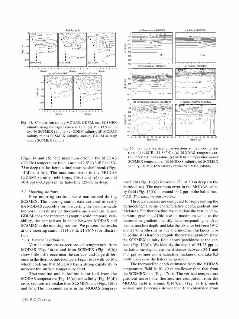
Vertical-time cross-sections of temperature fromMODAS (Fig. 16(a)) and from SCSMEX (Fig. 16(b))show little difference near the surface, and large differ-ence in the thermocline (compare Figs. 16(a) with 16(b)),which confirms that MODAS has a strong capability tonowcast the surface temperature field.

Thermocline and halocline identified from theMODAS temperature (Fig. 16(a)) and salinity (Fig. 16(d))cross-sections are weaker than SCSMEX data (Figs. 16(b)and (e)). The maximum error in the MODAS tempera-

ture field (Fig. 16(c)) is around 2°C at 50 m deep (in thethermocline). The maximum error in the MODAS salin-ity field (Fig. 16(f)) is around –0.2 ppt in the halocline.7.2.2 Thermocline parameters

Three parameters are computed for representing thethermocline/halocline characteristics: depth, gradient, andthickness. For thermocline, we calculate the vertical tem-perature gradient, ∂T/∂z, use its maximum value as thethermocline gradient, identify the corresponding depth asthe thermocline depth, and take the distance between 19°Cand 28°C isotherms as the thermocline thickness. Forhalocline, it is hard to compute the vertical gradient sincethe SCSMEX salinity field shows patchiness at the sur-face (Fig. 16(e)). We identify the depth of 34.25 ppt asthe halocline depth, use the distance between 34.1 and34.4 ppt isolines as the halocline thickness, and take 0.3ppt/thickness as the halocline gradient.

The thermocline depth estimated from the MODAStemperature field is 10–40 m shallower than that fromthe SCSMEX data (Fig. 17(a)). The vertical temperaturegradient across the thermocline computed from theMODAS field is around 0.14°C/m (Fig. 17(b)), muchweaker and (varying) slower than that calculated from

1 2 3 4 5 6 7 8 9 10−250

−200

−150

−100

−50

0

34.5

34.434.3

3433.8

33.633.5

(a) MODAS

Station

Dep

th (

m)

1 2 3 4 5 6 7 8 9 10

34.6

34.634.5

34.1

33.934.1

(b) SCSMEX

Station

Salinity (ppt)

1 2 3 4 5 6 7 8 9 10

34.6

34.5

34.434.3

34.234.1

33.933.7

(c) GDEM

Station

1 2 3 4 5 6 7 8 9 10−250

−200

−150

−100

−50

0

−0.1

−0.2

−0.3 −0.4

−0.4

−0.4

Station

Dep

th (

m)

(d) MODAS−SCSMEX

1 2 3 4 5 6 7 8 9 10

−0.1

−0.1

0

−0.3−0.3

−0.2 −0.4

(e) GDEM−SCSMEX

Station

−400

−350

−300

−250

−200

−150

−100

−50

0302826

2422

2018

16

14

12

dept

h(m

)

(a) Temperature (MODAS)

−500

−400

−300

−200

−100

0

100

3028 26 22 24

2018

16

14

12

10

dept

h(m

)

(b) Temperature (SCSMEX)

6 8 10 12 14 16 18 20 22 24 26−400

−350

−300

−250

−200

−150

−100

−50

0

0

0

0.5

0.5

−0.5−2−0.5

dept

h(m

)

date in Jul

(c) Temperature (MODAS−SCSMEX)

33.834

34.4

34.55

34.55

34.5

(d) Salinity (MODAS)

34.35

34.4

34.45

34.35

3434.05

(e) Salinity (SCSMEX)

6 8 10 12 14 16 18 20 22 24 26

0.125

0.1

−0.05−0.05

0.15

(f) Salinity (MODAS−SCSMEX)

date in Jul

Fig. 15. Comparison among MODAS, GDEM, and SCSMEXsalinity along the lag-C cross-section: (a) MODAS salin-ity, (b) SCSMEX salinity, (c) GDEM salinity, (d) MODASsalinity minus SCSMEX salinity, and (e) GDEM salinityminus SCSMEX salinity.

Fig. 16. Temporal-vertical cross-sections at the mooring sta-tion (114.38°E, 21.86°N): (a) MODAS temperature,(b) SCSMEX temperature, (c) MODAS temperature minusSCSMEX temperature, (d) MODAS salinity, (e) SCSMEXsalinity, (f) MODAS salinity minus SCSMEX salinity.

Evaluation of the U.S. Navy’s MODAS Model 1019

the SCSMEX data (0.19°–0.27°C/m). The thermoclinethickness computed from the MODAS field varies slowlyaround 80 m, which is lower in its temporal variation cal-culated from the SCSMEX data (40–100 m).

7.2.3 Halocline parametersWe computed three parameters to represent the

halocline characteristics: halocline depth, salinity gradi-ent across the halocline, and halocline thickness. Thehalocline depth estimated from the MODAS salinity fieldis always deeper than that from the SCSMEX data (Fig.17(d)). The vertical salinity gradient across the haloclinecomputed from the MODAS field is around 0.011 ppt/m(Fig. 17(e)), which is generally stronger than that calcu-lated from the SCSMEX data (0.0065–0.011 ppt/m). Thehalocline thickness computed from the MODAS fieldvaries slowly around 30 m, which is generally thinnerthan that calculated from the SCSMEX data (28–46 m).

8. Future MODAS Improvement

8.1 MODAS first special treatmentTemperature (salinity) profiles in oceans usually ex-

hibit a multi-layer structure consisting of mixed-layer,thermocline (halocline), and two deep layers. When thetwo deep layers have the same vertical gradients, theybecome one deep layer. The vertical thermal structure (i.e.,depths and gradients) changes in space and time. Six lay-ers can represent vertical thermal structure if the entrain-ment zone between the mixed layer and thermocline andthe transition zone between the thermocline and the deeplayer are added (Fig. 18). Each observed profile is repre-sented by a set of parameters, most of which have physi-cal meaning, including SST, mixed layer depth (MLD),depth of the base of the thermocline, gradient in thethermocline and deep layers, and additional parametersdescribing vertical gradients (Chu et al., 1997c, 1999b,2000). For a vertically uniform temperature profile, MLDequals the water depth and thermocline gradient equalszero. Each observed profile is represented by depths andgradients of each layer: H (water depth), d1 (MLD), d2(depth of the thermocline top), d3 (depth of thethermocline bottom), d4 (depth of the top of the first deeplayer), and d5 (bottom of the first deep layer), G(m) (~0,mixed layer gradient), G(th) (large, thermocline gradient),G(tr) (mean entrainment zone gradient), G(d1) (mean gra-dient in the first deep layer), and G(d2) (mean gradient inthe second deep layer). Here, the mean entrainment zonegradient is the average of the mixed layer and thermoclinegradients.

The depths (d1, d2, d3, d4, d5) and gradients [G(m),G(th), G(tr), G(d1), G(d2)] represent characteristics of tem-perature profiles that vary in space and time. It is diffi-cult and unrealistic to archive these characteristics fromSST and SSH using the MODAS first treatment. In fu-ture MODAS, the synthetic temperature profiles will beobtained from the relationships between (SST, SSH) and(d1, d2, d3, d4, d5), gradients [G(m), G(th), G(tr), G(d1), G(d2)],rather than from the relationships between (SST, SSH)and temperature at given depth (MODAS first treatment).

Fig. 18. Characteristics of vertical temperature structure:(a) profile, and (b) gradient.

Fig. 17. Thermocline and halocline parameters determined fromMODAS (dashed) and SCSMEX (solid) at the mooring sta-t ion (114.38°E, 21.86°N): (a) thermocline depth,(b) thermocline gradient, (c) thermocline thickness,(d) halocline depth, (e) halocline gradient, and (f) haloclinethickness.

−65

−60

−55

−50

−45

−40

−35

−30

ther

moc

line

dept

h(m

)

(a)

MODAS SCSMEX

0.12

0.14

0.16

0.18

0.2

0.22

0.24

0.26

0.28

tem

pera

ture

gra

dien

t(c/

m)

(b)

MODAS SCSMEX

6 8 10 12 14 16 18 20 22 24 2640

50

60

70

80

90

100

110

ther

moc

line

thic

knes

s(m

)

date in July

(c)

MODAS SCSMEX

−85

−80

−75

−70

−65

−60

halo

clin

e de

pth(

m)

(d)

MODAS SCSMEX

0.006

0.007

0.008

0.009

0.01

0.011

0.012

0.013

0.014sa

linity

gra

dien

t(pp

t/m)

(e)

MODAS SCSMEX

6 8 10 12 14 16 18 20 22 24 2620

25

30

35

40

45

50

halo

clin

e th

ickn

ess(

m)

date in July

(f)

MODAS SCSMEX

SST

T(z)

Z

d1 G(m)

d2

G(th)

d3G(tr)

d4

G(d1)

d5

G(d2)

(−) 0 (+)

H

∂T/∂z

1020 P. C. Chu et al.

8.2 MODAS second special treatmentThe assumption underlying the MODAS second

treatment is the existence of a dependence of salinitysolely on temperature. Chu and Garwood (1990, 1991)and Chu et al. (1990) found a two-phase thermodynam-ics of atmosphere and ocean, each medium having twoindependent variables: temperature and salinity foroceans, temperature and humidity (or cloud fraction) forthe atmosphere. Both positive and negative feedbackmechanisms are available between atmosphere and ocean.First, clouds reduce the incoming solar radiation at theocean surface by scattering and absorption, which cools(relatively) the ocean mixed layer. The cooling of theocean mixed layer lowers the evaporation rate, which willdiminish the clouds. This is the negative feedback. Sec-ond, precipitation dilutes the surface salinity, stabilizingthe upper ocean and reducing ocean mixed layer deepen-ing. The MLD may be caused to shallow if the downwardsurface buoyancy flux is sufficiently enhanced by the pre-cipitation. The reduction in MLD will increase SST byconcentrating the net radiation plus heat flux downwardacross the sea surface into thinner layer. The increase ofSST augments the surface evaporation, which increasesthe surface salinity (for ocean) and produces more clouds(for atmosphere). This indicates that no unique T-S rela-tionship exists, especially in the upper ocean.

A reasonable way to represent salinity profile is bydepths and gradients: d1 (MLD for salinity), d2 (depth ofthe halocline top), d3 (depth of the halocline bottom), d4(depth of the top of the first deep layer), and d5 (bottomof the first deep layer), GS

(m) (~0, mixed layer gradient),GS

(ha) (halocline gradient), GS(tr) (mean entrainment zone

gradient), GS(d1) (mean gradient in the first deep layer),

and GS(d2) (mean gradient in the second deep layer). In a

future MODAS, synthetic salinity profiles should be in-dependent of the synthetic temperature profiles. They willbe obtained from the relationships between surface data(SST, SSH, precipitation) and (d1, d2, d3, d4, d5), [GS

(m),GS

(ha), GS(tr), GS

(d1), GS(d2)].

9. Conclusions(1) MODAS has the capability to provide reason-

ably good temperature and salinity nowcast fields. Theerrors have a Gaussian-type distribution with mean tem-perature nearly zero and mean salinity of –0.2 ppt. Thestandard deviations of temperature and salinity errors are0.98°C and 0.22 ppt, respectively.

(2) The skill score of the temperature nowcast ispositive, except at depths between 1750 and 2250 m. Theskill score of the salinity nowcast is less than that of thetemperature nowcast, especially at depths between 300and 400 m, where the skill score is negative.

(3) The MODAS mean temperature is slightly(0.1°C) cooler than the SCSMEX mean temperature at

the surface. Below 30 m deep, the MODAS mean tem-perature becomes warmer than the SCSMEX mean tem-perature with the maximum bias (about 0.6°C warmer) at100 m deep. Below 100 m depth, the warm bias decreaseswith depth to less than 0.1°C below 500 m deep.

(4) The MODAS mean salinity is less than theSCSMEX mean salinity at all depths, which indicates thatthe MODAS under-estimates the salinity field. Such a biasincreases with depth from 0.113 ppt at the surface to amaximum value of 0.135 ppt at 60 m depth and decreaseswith depth below 60 m deep.

(5) Thermocline and halocline identified from theMODAS temperature and salinity fields are weaker thanthe SCSMEX data. The maximum discrepancy betweenthe two is in the thermocline and halocline. In outcroppinghalocline, the discrepancy becomes high (0.7 ppt alongLag-B).

(6) The thermocline depth estimated from theMODAS temperature field is 10–40 m shallower than thatfrom the SCSMEX data. The vertical temperature gradi-ent across the thermocline computed from the MODASfield is around 0.14°C/m, which is much weaker than thatcalculated from the SCSMEX data (0.19°–0.27°C/m). Thethermocline thickness computed from the MODAS fieldvaries slowly around 80 m, which falls in its temporalvariation calculated from the SCSMEX data (40–100 m).

(7) The halocline depth estimated from the MODASsalinity field is deeper than that from the SCSMEX data.Its thickness computed from the MODAS field variesslowly around 30 m, which is generally thinner than thatcalculated from the SCSMEX data (28–46 m).

(8) MODAS has two special treatments for creat-ing synthetic temperature and salinity profiles. The firstone is to use linear regression relationships between (SST,SSH) with temperature at a given depth. The second oneis to assume that salinity is a sole function of tempera-ture and to derive synthetic salinity profiles from syn-thetic temperature profiles. In a future MODAS, the syn-thetic temperature profiles should be obtained from therelationships between (SST, SSH) and depths-tempera-ture gradients; and synthetic salinity profiles should beobtained from the relationships between surface data(SST, SSH, precipitation) and depths-salinity gradients.

AcknowledgementsThe authors wish to thank Dan Fox of the Naval

Research Laboratory at Stennis Space Center for mostkindly providing MODAS T, S fields. The Office of Na-val Research, the Naval Oceanographic Office, and theNaval Postgraduate School funded this work.

ReferencesCai, S. Q., J.-L. Su, Z. J. Gan and Q. Y. Liu (2002): The nu-

merical study of the South China Sea upper circulation char-

Evaluation of the U.S. Navy’s MODAS Model 1021

acteristics and its dynamic mechanism in winter. Cont. ShelfRes., 22, 2247–2264.

Carnes, M., L. Mitchell and P. W. deWitt (1990): Synthetic tem-perature profiles derived from Geosat altimetry: Compari-son with air-dropped expendable bathythermograph profiles.J. Geophys. Res., 95(C10), 17979–17992.

Carnes, M., R. D. Fox and R. Rhodes (1996): Data assimilationin a north Pacific ocean monitoring and prediction system.p. 319–345. In Modern Approaches to Data Assimilation inOcean Modeling, ed. by P. Malanote-Rizzoli, Elsivier.

Chao, S. Y., P. T. Shaw and J. Wang (1996): Deep water venti-lation in the South China Sea. Deep-Sea Res., 43, 445–466.

Chu, P. C. and R. W. Garwood, Jr. (1990): Thermodynamic feed-back between cloud and ocean mixed layer. Adv. Atmos. Sci.,7, 1–10.

Chu, P. C. and R. W. Garwood, Jr. (1991): On the two-phasethermodynamics of the coupled cloud-ocean mixed layer.J. Geophys. Res., 96, 3425–3436.

Chu, P. C. and G. H. Wang (2003): Seasonal variability ofthermohaline front in the central South China Sea. J.Oceanogr., 59, 65–78.

Chu, P. C., R. W. Garwood, Jr. and P. Muller (1990): Unstableand damped modes in coupled ocean mixed layer and cloudmodels. J. Mar. Sys., 1, 1–11.

Chu, P. C., H. C. Tseng, C. P. Chang and J. M. Chen (1997a):South China Sea warm pool detected in spring from theNavy’s Master Oceanographic Observational Data Set(MOODS). J. Geophys. Res., 102, 15761–15771.

Chu, P. C., S. H. Lu and Y. Chen (1997b): Temporal and spatialvariabilities of the South China Sea surface temperatureanomaly. J. Geophys. Res., 102, 20937–20955.

Chu, P. C., C. R. Fralick, S. D. Haeger and M. J. Carron (1997c):A parametric model for Yellow Sea thermal variability. J.Geophys. Res., 102, 10499–10508.

Chu, P. C., C. Fan, C. J. Lozano and J. L. Kerling (1998): Anairborne expandable bathythermograph survey of the SouthChina Sea, May 1995. J. Geophys. Res., 103, 21637–21652.

Chu, P. C., N. L. Edmons and C. W. Fan (1999a): Dynamicalmechanisms for the South China Sea seasonal circulation

and thermohaline variabilities. J. Phys. Oceanogr., 29,2971–2989.

Chu, P. C., Q. Q. Wang and R. H. Bourke (1999b): A geometricmodel for Beaufort/Chukchi Sea thermohaline structure. J.Atmos. Oceanic Technol., 16, 613–632.

Chu, P. C., C. W. Fan and W. T. Liu (2000): Determination ofsub-surface thermal structure from sea surface temperature.J. Atmos. Oceanic Technol., 17, 971–979.

Chu, P. C., S. H. Lu and Y. C. Chen (2001): Evaluation of thePrinceton Ocean Model using the South China Sea MonsoonExperiment (SCSMEX) data. J. Atmos. Oceanic Technol.,18, 1521–1539.

Fox, D. N., W. J. Teague, C. N. Barron, M. R. Carnes and C. M.Lee (2002): The modular ocean data assimilation system(MODAS). J. Atmos. Oceanic Technol., 19, 240–252.

Isobe, A. and T. Namba (2001): The circulation in the upperand intermediate layers of the South China Sea. J.Oceanogr., 57, 93–104.

Levitus, S. and T. Boyer (1994a): Temperature. Vol. 4, WorldOcean Atlas 1994, NOAA Atlas NESDIS 4, 150 pp.

Levitus, S., and T. Boyer (1994b): Salinity. Vol. 3, World OceanAtlas 1994, NOAA Atlas NESDIS 3, 150 pp.

Murphy, A. H. (1988): Skill score based on the mean squareerror and their relationships to the correlation coefficient.Mon. Weather Rev., 116, 2417–2424.

NAVOCEANO (1999): Operational Test (OPTEST) Report forthe Modular Ocean Data Assimilation System (MODAS)Version 2.1. Naval Oceanographic Office, Stennis SpaceCenter, Mississippi, p. 40.

SCSMEX Science Working Group (1995): The South China SeaMonsoon Experiment (SCSMEX) Science Plan. NASA/Goddard Space Flight Center, Greenbelt, Maryland, 65 pp.

Teague, W. J., M. J. Carron and P. J. Hogan (1990): A compari-son between the Generalized Digital Environmental Modeland Levitus climatologies. J. Geophys. Res., 95, 7167–7183.

Wyrtki, K. (1961): Scientific results of marine investigationsof the South China Sea and the Gulf of Thailand 1959–1961.Naga Report, Vol. 2, 195 pp.