Embed Size (px)
Citation preview
European Conference on Computational Fluid DynamicsECCOMAS CFD 2006
P. Wesseling, E. Onate and J. Periaux (Eds)c© TU Delft, The Netherlands, 2006
EVALUATION OF THE SST-SAS MODEL: CHANNELFLOW, ASYMMETRIC DIFFUSER AND AXI-SYMMETRIC
HILL
Lars Davidson
Division of Fluid Dynamics, Department of Applied MechanicsChalmers University of Technology, SE-412 96 Goteborg, Sweden
e-mail: [email protected]
Key words: von Karman length scale, unsteady, URANS, DES, LES, scale-adapted
Abstract. The SAS model (Scale Adapted Simulation) was invented by Menter and co-workers. The idea behind the SST-SAS k − ω model is to add an additional productionterm – the SAS term – in the ω equation, which is sensitive to resolved (i.e. unsteady)fluctuations. When the flow equations resolve turbulence, the length scale based on velocitygradients is much smaller than that based on time-averaged velocity gradients. Hence thevon Karman length scale, LvK , is an appropriate quantity to use as a sensor for detectingunsteadiness. In regions where the flow is on the limit of going unsteady, the objective ofthe SAS term is to increase ω. The result is that k and νt are reduced so that the dissipating(damping) effect of the turbulent viscosity on the resolved fluctuations is reduced, therebypromoting the momentum equations to switch from steady to unsteady mode.
The SST-SAS model and the standard SST-URANS are evaluated for three flows: de-veloping channel flow, the flow in an asymmetric, plane diffuser and the flow around athree-dimensional axi-symmetric hill. Unsteady inlet boundary conditions are prescribedin all cases by superimposing turbulent fluctuations on a steady inlet boundary velocityprofile.
1 Introduction
1st line after Eq. 4 corrected
RANS turbulence models, such as two-equation eddy-viscosity models, are highly dis-sipative. This means that they are not likely to be triggered into unsteady mode unlessthe flow instabilities are strong (such as vortex shedding behind bluff bodies [1–3]). It isa good idea in many flow situations to let the RANS solution go unsteady. First, on afine mesh, it may well be that no steady solution exists. In that case there is no pointin trying to force the flow to a steady solution. Second, if some large movements (eitherthe very largest turbulence structures or some quasi-periodic non-turbulent structure) areallowed to be resolved, the flow will be more accurately captured. In a way, this is theidea of DES [4, 5], in which the turbulence in the boundary layers is modelled (RANS)
1
Lars Davidson
0 5 10 15 200
0.2
0.4
0.6
0.8
1
PSfrag replacements
U+
y
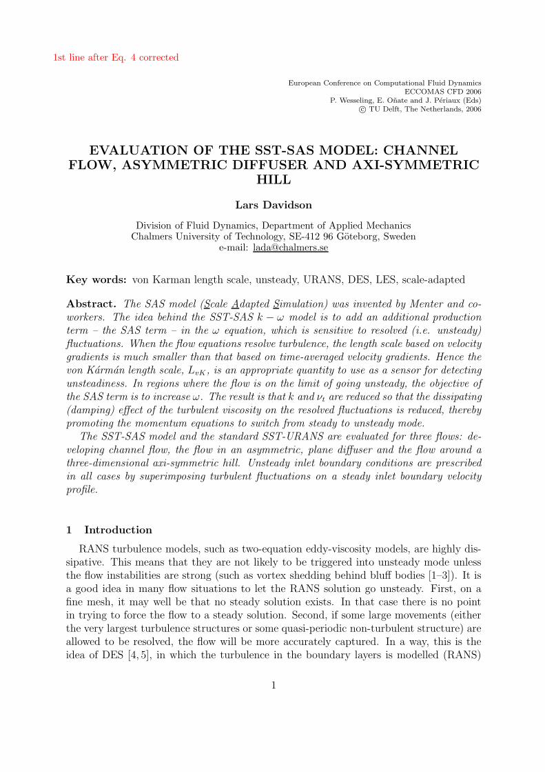
Figure 1: Velocity profiles from a DNS of channel flow. Solid line: time-averaged velocity; dashed line:instantaneous velocity.
and the large detached eddies are resolved (LES). In DES, the switch between the RANSand LES is dictated by the ratio of the RANS to the LES turbulent length scales. Thelatter length scale is defined from the grid (the length of the largest cell side).
The present work evaluates a new approach by Menter and co-workers [6–8] called SAS(Scale-Adapted Simulation). The SAS term is an additional production term in the ωequation that increases when the flow equations start to go unsteady. The SAS termswitches itself on when the ratio of the modelled turbulent length scale, k1/2/ω, to thevon Karman length scale increases. The von Karman length scale, which is based onthe ratio of the first to the second velocity gradients, is smaller for an unsteady velocityprofile than for a steady velocity profile, see Fig. 1. The idea of the SAS term is that,when the flow equations resolve unsteadiness, the SAS term detects the unsteadiness andincreases the production of ω. The effect is that ω increases, and hence the turbulentviscosity decreases because ω appears in the denominator in the expression for νt andbecause the magnitude of the destruction term, −β∗kω, in the modelled turbulent kineticenergy equation increases.
It should be mentioned that the usage of the SAS model in this work is somewhatdifferent from the intended usage, as SAS is intended for flow-regions which are inherentlyunsteady. In this work the model is also tested for its performance with respect to flowswhere the boundary layer turbulence is partly resolved.
The paper is organised as follows. First, the SST-SAS k − ω model is derived. Inthe next section, the von Karman is evaluated using instantaneous channel data obtainedby DNS (fine mesh) and hybrid LES-RANS (coarse mesh). The numerical method andthe instantaneous inlet boundary conditions are then briefly presented. The results arereported and discussed, and, finally, conclusions are drawn.
2
Lars Davidson
2 The k − kL Turbulence Model
2.1 Derivation
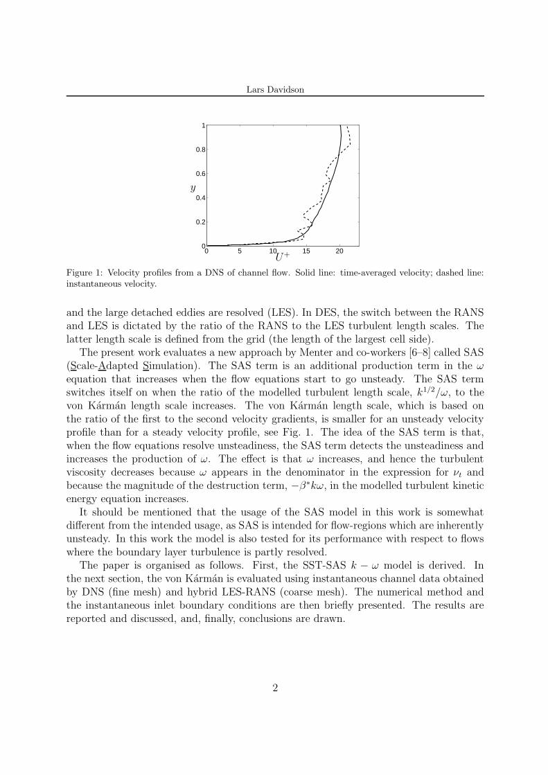
Rotta [9] derived an exact equation for kL based on the integral length scale.
kL =3
16
∫
Rii(x, η)dη, Rij = ui(x)uj(x + η) (1)
All two-equation models have one production term and one destruction term. Rotta’s kLequation includes two production terms, namely (here given in boundary-layer form)
SkL = − 3
16
∂u(x)
∂y
∫
R21dη︸ ︷︷ ︸
I
− 3
16
∫∂u(x + η)
∂yR12dη
︸ ︷︷ ︸
II
(2)
To simplify the second term, Rotta used Taylor expansion so that
∂u(x + η)
∂y=
∂u(x)
∂y︸ ︷︷ ︸
a
+ η∂2u(x)
∂y2
︸ ︷︷ ︸
b
+1
2η2∂3u(x)
∂y3
︸ ︷︷ ︸
c
+ . . . (3)
The first term, a, is incorporated in SkL,I . Rotta set the second term, b, to zero
∂2u(x)
∂y2
∫ +∞
−∞
R12ηdη = 0 (4)
because, in homogeneous shear flow, R12(η) is symmetric with respect to η. The secondterm in Eq. 2 was consequently modelled with the third term, c, including the thirdvelocity gradient ∂3u/∂y3.
Menter & Egorov [7] argue that homogeneous shear flow is not a relevant flow casebecause the second velocity gradient here is zero anyway. They propose modelling theSkL,II term in Eq. 2 using the second velocity gradient as [7, 8]:
SkL,IIb = − 3
16
∫∂u(x + η)
∂yR12dη = −c |uv|
∣∣∣∣
∂2u(x)
∂y2
∣∣∣∣L2 (5)
The eddy-viscosity assumption for the shear stress gives |uv| = νt|∂u/∂y|. In three-dimensional flow the shear stress can be estimated by an eddy-viscosity expression, νt(2sij sij)
1/2.Using a general formula for the second derivative of the velocity we get [7, 8]
SkL,IIb = −νtS |U ′′|L2
S = (2sij sij)1/2
U ′′ =
(∂2ui
∂xj∂xj
∂2ui
∂xk∂xk
)1/2(6)
3
Lars Davidson
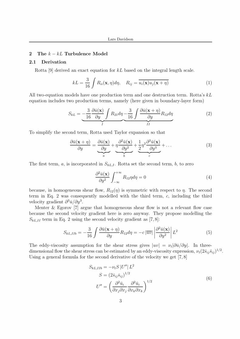
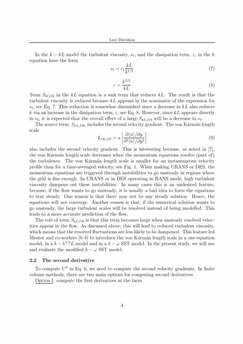
In the k − kL model the turbulent viscosity, νt, and the dissipation term, ε, in the kequation have the form
νt = c1kL
k1/2(7)
ε =k5/2
kL(8)
Term Skl,IIb in the kL equation is a sink term that reduces kL. The result is that theturbulent viscosity is reduced because kL appears in the nominator of the expression forνt, see Eq. 7. This reduction is somewhat diminished since a decrease in kL also reducesk via an increase in the dissipation term, ε, see Eq. 8. However, since kL appears directlyin νt, it is expected that the overall effect of a large SkL,IIb will be a decrease in νt.
The source term, SkL,IIb, includes the second velocity gradient. The von Karman lengthscale
LvK,1D = κ
∣∣∣∣
∂〈u〉/∂y
∂2〈u〉/∂y2
∣∣∣∣
(9)
also includes the second velocity gradient. This is interesting because, as noted in [7],the von Karman length scale decreases when the momentum equations resolve (part of)the turbulence. The von Karman length scale is smaller for an instantaneous velocityprofile than for a time-averaged velocity, see Fig. 1. When making URANS or DES, themomentum equations are triggered through instabilities to go unsteady in regions wherethe grid is fine enough. In URANS or in DES operating in RANS mode, high turbulentviscosity dampens out these instabilities. In many cases this is an undesired feature,because, if the flow wants to go unsteady, it is usually a bad idea to force the equationsto stay steady. One reason is that there may not be any steady solution. Hence, theequations will not converge. Another reason is that, if the numerical solution wants togo unsteady, the large turbulent scales will be resolved instead of being modelled. Thisleads to a more accurate prediction of the flow.
The role of term SkL,IIb is that this term becomes large when unsteady resolved veloc-ities appear in the flow. As discussed above, this will lead to reduced turbulent viscosity,which means that the resolved fluctuations are less likely to be dampened. This feature ledMenter and co-workers [6–8] to introduce the von Karman length scale in a one-equationmodel, in a k − k1/2L model and in a k − ω SST model. In the present study, we will useand evaluate the modified k − ω SST model.
2.2 The second derivative
To compute U ′′ in Eq. 6, we need to compute the second velocity gradients. In finitevolume methods, there are two main options for computing second derivatives.
Option I: compute the first derivatives at the faces
4
Lars Davidson
(∂u
∂y
)
j+1/2
=uj+1 − uj
∆y,
(∂u
∂y
)
j−1/2
=uj − uj−1
∆y
and then
⇒(
∂2u
∂y2
)
j
=uj+1 − 2uj + uj−1
(∆y)2+
(∆y)2
12
∂4u
∂y4
Option II: compute the first derivatives at the center
(∂u
∂y
)
j+1
=uj+2 − uj
2∆y,
(∂u
∂y
)
j−1
=uj − uj−2
2∆y
and then
⇒(
∂2u
∂y2
)
j
=uj+2 − 2uj + uj−2
4(∆y)2+
(∆y)2
3
∂4u
∂y4
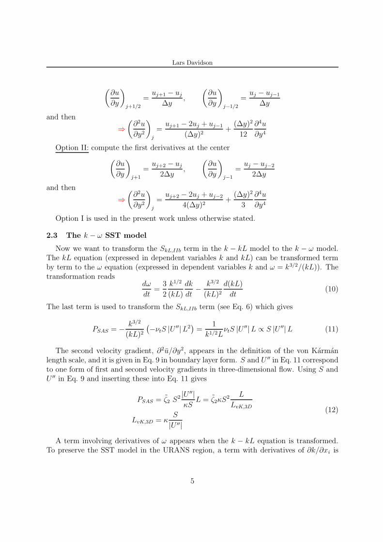
Option I is used in the present work unless otherwise stated.
2.3 The k − ω SST model
Now we want to transform the SkL,IIb term in the k − kL model to the k − ω model.The kL equation (expressed in dependent variables k and kL) can be transformed termby term to the ω equation (expressed in dependent variables k and ω = k3/2/(kL)). Thetransformation reads
dω
dt=
3
2
k1/2
(kL)
dk
dt− k3/2
(kL)2
d(kL)
dt(10)
The last term is used to transform the SkL,IIb term (see Eq. 6) which gives
PSAS = − k3/2
(kL)2
(−νtS |U ′′|L2
)=
1
k1/2LνtS |U ′′|L ∝ S |U ′′|L (11)
The second velocity gradient, ∂2u/∂y2, appears in the definition of the von Karmanlength scale, and it is given in Eq. 9 in boundary layer form. S and U ′′ in Eq. 11 correspondto one form of first and second velocity gradients in three-dimensional flow. Using S andU ′′ in Eq. 9 and inserting these into Eq. 11 gives
PSAS = ζ2 S2 |U ′′|κS
L = ζ2κS2 L
LvK,3D
LvK,3D = κS
|U ′′|
(12)
A term involving derivatives of ω appears when the k − kL equation is transformed.To preserve the SST model in the URANS region, a term with derivatives of ∂k/∂xi is
5
Lars Davidson
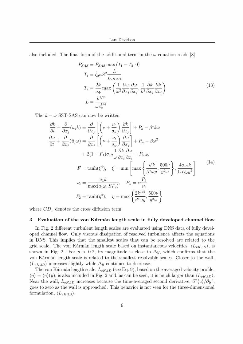
also included. The final form of the additional term in the ω equation reads [8]
PSAS = FSAS max (T1 − T2, 0)
T1 = ζ2κS2 L
LvK,3D
T2 =2k
σΦmax
(1
ω2
∂ω
∂xj
∂ω
∂xj,
1
k2
∂k
∂xj
∂k
∂xj
)
L =k1/2
ωc1/4µ
(13)
The k − ω SST-SAS can now be written
∂k
∂t+
∂
∂xj(ujk) =
∂
∂xj
[(
ν +νt
σk
)∂k
∂xj
]
+ Pk − β∗kω
∂ω
∂t+
∂
∂xj(ujω) =
∂
∂xj
[(
ν +νt
σω
)∂ω
∂xj
]
+ Pω − βω2
+ 2(1 − F1)σω21
ω
∂k
∂xi
∂ω
∂xi+ PSAS
F = tanh(ξ4), ξ = min
[
max
{ √k
β∗ωy,500ν
y2ω
}
,4σω2k
CDωy2
]
νt =a1k
max(a1ω, SF2), Pω = α
Pk
νt
F2 = tanh(η2), η = max
{2k1/2
β∗ωy,500ν
y2ω
}
(14)
where CDω denotes the cross diffusion term.
3 Evaluation of the von Karman length scale in fully developed channel flow
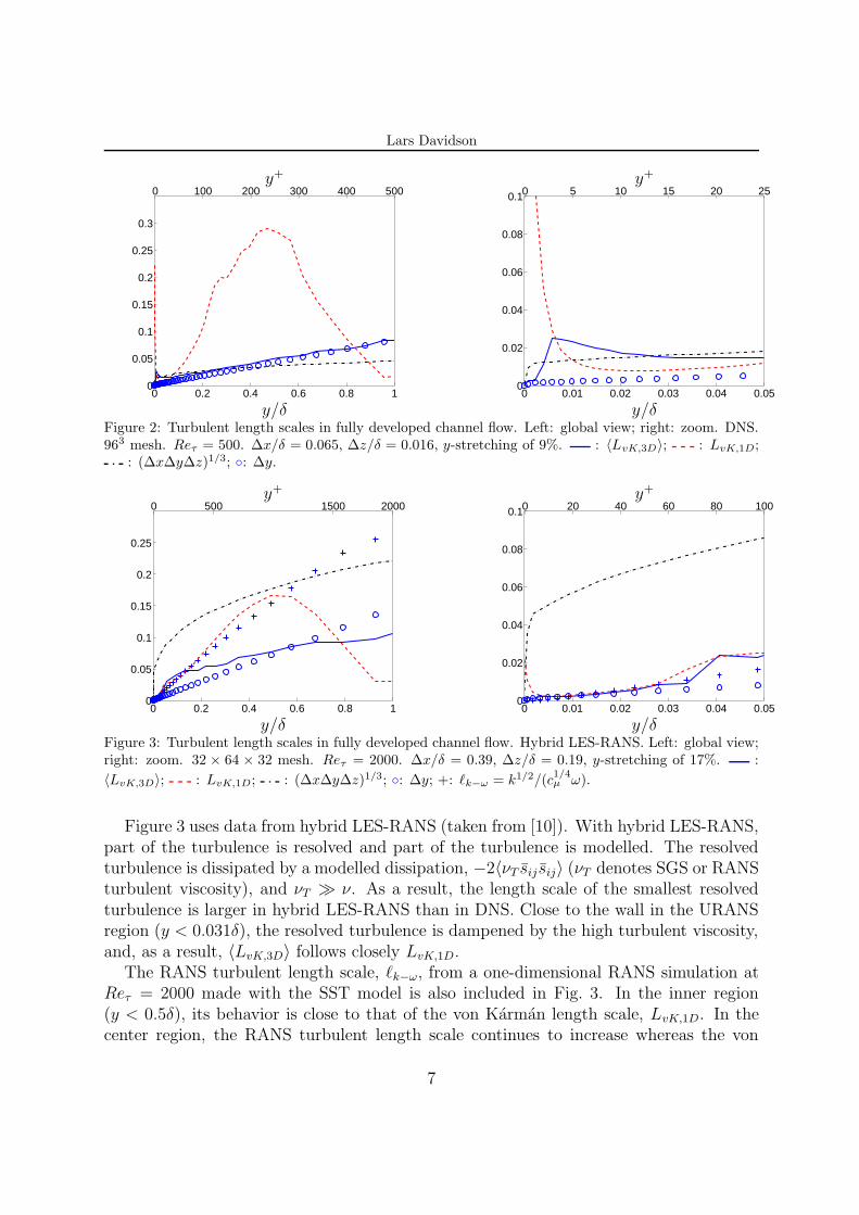
In Fig. 2 different turbulent length scales are evaluated using DNS data of fully devel-oped channel flow. Only viscous dissipation of resolved turbulence affects the equationsin DNS. This implies that the smallest scales that can be resolved are related to thegrid scale. The von Karman length scale based on instantaneous velocities, 〈LvK,3D〉, isshown in Fig. 2. For y > 0.2, its magnitude is close to ∆y, which confirms that thevon Karman length scale is related to the smallest resolvable scales. Closer to the wall,〈LvK,3D〉 increases slightly while ∆y continues to decrease.
The von Karman length scale, LvK,1D (see Eq. 9), based on the averaged velocity profile,〈u〉 = 〈u〉(y), is also included in Fig. 2 and, as can be seen, it is much larger than 〈LvK,3D〉.Near the wall, LvK,1D increases because the time-averaged second derivative, ∂2〈u〉/∂y2,goes to zero as the wall is approached. This behavior is not seen for the three-dimensionalformulation, 〈LvK,3D〉.
6
Lars Davidson
0 0.2 0.4 0.6 0.8 10
0.05
0.1
0.15
0.2
0.25
0.3
0 100 200 300 400 500
PSfrag replacements
y/δ
y+
0 0.01 0.02 0.03 0.04 0.050
0.02
0.04
0.06
0.08
0.10 5 10 15 20 25
PSfrag replacements
y/δ
y+
Figure 2: Turbulent length scales in fully developed channel flow. Left: global view; right: zoom. DNS.963 mesh. Reτ = 500. ∆x/δ = 0.065, ∆z/δ = 0.016, y-stretching of 9%. : 〈LvK,3D〉; : LvK,1D;
: (∆x∆y∆z)1/3; ◦: ∆y.
0 0.2 0.4 0.6 0.8 10
0.05
0.1
0.15
0.2
0.25
0 500 1500 2000
PSfrag replacements
y/δ
y+
0 0.01 0.02 0.03 0.04 0.050
0.02
0.04
0.06
0.08
0.10 20 40 60 80 100
PSfrag replacements
y/δ
y+
Figure 3: Turbulent length scales in fully developed channel flow. Hybrid LES-RANS. Left: global view;right: zoom. 32 × 64 × 32 mesh. Reτ = 2000. ∆x/δ = 0.39, ∆z/δ = 0.19, y-stretching of 17%. :
〈LvK,3D〉; : LvK,1D; : (∆x∆y∆z)1/3; ◦: ∆y; +: `k−ω = k1/2/(c1/4µ ω).
Figure 3 uses data from hybrid LES-RANS (taken from [10]). With hybrid LES-RANS,part of the turbulence is resolved and part of the turbulence is modelled. The resolvedturbulence is dissipated by a modelled dissipation, −2〈νT sij sij〉 (νT denotes SGS or RANSturbulent viscosity), and νT � ν. As a result, the length scale of the smallest resolvedturbulence is larger in hybrid LES-RANS than in DNS. Close to the wall in the URANSregion (y < 0.031δ), the resolved turbulence is dampened by the high turbulent viscosity,and, as a result, 〈LvK,3D〉 follows closely LvK,1D.
The RANS turbulent length scale, `k−ω, from a one-dimensional RANS simulation atReτ = 2000 made with the SST model is also included in Fig. 3. In the inner region(y < 0.5δ), its behavior is close to that of the von Karman length scale, LvK,1D. In thecenter region, the RANS turbulent length scale continues to increase whereas the von
7
Lars Davidson
Karman length scale, LvK,1D, goes to zero.Two filter scales are included in Figs. 2 and 3. In the DNS simulations, ∆y <
(∆x∆y∆z)1/3 near the wall; far from the wall, however, ∆y > (∆x∆y∆z)1/3 becauseof both the stretching in the y direction and small ∆x and ∆z. In the hybrid simulations,it can be noted that the three-dimensional filter width is approximately twice as large asthe three-dimensional formulation of the von Karman length scale, i.e. (∆x∆y∆z)1/3 >〈LvK,3D〉.
4 The Numerical Method
An incompressible, finite volume code with a non-staggered grid arrangement is used [11].For space discretization, central differencing is used for all terms. The Crank-Nicholsonscheme is used for time discretization of all equations. The numerical procedure is basedon an implicit, fractional step technique with a multigrid pressure Poisson solver [12].
5 Inlet Conditions
For the channel simulations inlet fluctuating velocity fields (u′, v′, w′) are created ateach time step at the inlet y − z plane using synthetic isotropic fluctuations [13, 14].These are independent of one another, however, and thus their time correlation will bezero. This is unphysical. To create correlation in time, new fluctuating velocity fields, U ′,V ′, W ′, are computed as [13, 15, 16]
(U ′)m = a(U ′)m−1 + b(u′)m
(V ′)m = a(V ′)m−1 + b(v′)m
(W ′)m = a(W ′)m−1 + b(w′)m
(15)
where m denotes time step number, a = exp(−∆t/T ) and b = (1 − a2)1/2. The timecorrelation of U ′
i will be equal to exp(−∆t/T ), where T is proportional to the turbulenttime scale. The inlet boundary conditions are prescribed as
u(0, y, z, t) = Uin(y) + u′in(y, z, t)
v(0, y, z, t) = v′in(y, z, t)
w(0, y, z, t) = w′in(y, z, t)
(16)
The mean inlet velocity, Uin(y), k and ω are taken from one-dimensional channel flowpredicted with the SST model.
For the diffuser flow simulations, the inlet conditions are taken from a DNS of fullydeveloped channel flow at Reτ = 500. k and ω are taken from one-dimensional channelflow obtained with the SST model.
For the three-dimensional hill simulations, fluctuations are taken from the same DNS ofchannel flow. These fluctuations are then re-scaled and superimposed on the experimentalmean inlet velocity profile. Neumann conditions are used for k and ω.
8
Lars Davidson
PSfrag replacements
inlet
outlet
2δ
x
y
100δ
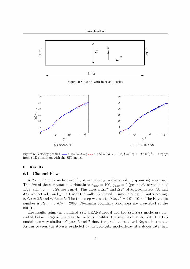
Figure 4: Channel with inlet and outlet.
101
102
103
0
5
10
15
20
25
30
PSfrag replacements
y+
〈u〉/
uτ,x
(a) SAS-SST
101
102
103
0
5
10
15
20
25
30
PSfrag replacements
y+
(b) SAS-URANS.
Figure 5: Velocity profiles. : x/δ = 3.33; : x/δ = 23; : x/δ = 97; +: 2.5 ln(y+) + 5.2; 5:from a 1D simulation with the SST model.
6 Results
6.1 Channel Flow
A 256 × 64 × 32 node mesh (x, streamwise; y, wall-normal; z, spanwise) was used.The size of the computational domain is xmax = 100, ymax = 2 (geometric stretching of17%) and zmax = 6.28, see Fig. 4. This gives a ∆x+ and ∆z+ of approximately 785 and393, respectively, and y+ < 1 near the walls, expressed in inner scaling. In outer scaling,δ/∆x ' 2.5 and δ/∆z ' 5. The time step was set to ∆tuτ/δ = 4.91 · 10−3. The Reynoldsnumber is Reτ = uτδ/ν = 2000. Neumann boundary conditions are prescribed at theoutlet.
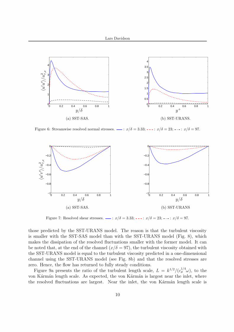
The results using the standard SST-URANS model and the SST-SAS model are pre-sented below. Figure 5 shows the velocity profiles; the results obtained with the twomodels are very similar. Figures 6 and 7 show the predicted resolved Reynolds stresses.As can be seen, the stresses predicted by the SST-SAS model decay at a slower rate than
9
Lars Davidson
0 0.2 0.4 0.6 0.8 10
1
2
3
4
PSfrag replacements〈u′ u
′ 〉/u
2 τ,x
y/δ
(a) SST-SAS.
0 0.2 0.4 0.6 0.8 10
0.5
1
1.5
2
2.5
3
3.5
4
PSfrag replacements
y+
(b) SST-URANS.
Figure 6: Streamwise resolved normal stresses. : x/δ = 3.33; : x/δ = 23; : x/δ = 97.
0 0.2 0.4 0.6 0.8 1−1
−0.8
−0.6
−0.4
−0.2
0
PSfrag replacements〈u′ v
′ 〉/u
2 τ,x
y/δ
(a) SST-SAS.
0 0.2 0.4 0.6 0.8 1−1
−0.8
−0.6
−0.4
−0.2
0
PSfrag replacements
y/δ
(b) SST-URANS
Figure 7: Resolved shear stresses. : x/δ = 3.33; : x/δ = 23; : x/δ = 97.
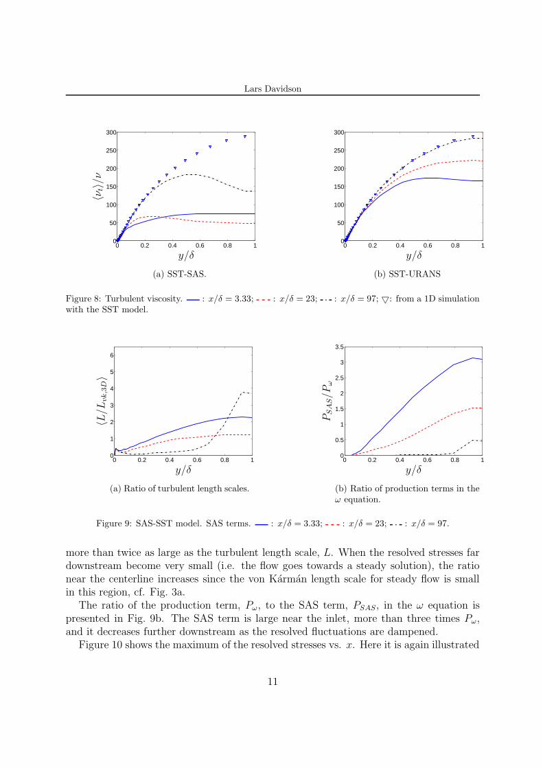
those predicted by the SST-URANS model. The reason is that the turbulent viscosityis smaller with the SST-SAS model than with the SST-URANS model (Fig. 8), whichmakes the dissipation of the resolved fluctuations smaller with the former model. It canbe noted that, at the end of the channel (x/δ = 97), the turbulent viscosity obtained withthe SST-URANS model is equal to the turbulent viscosity predicted in a one-dimensionalchannel using the SST-URANS model (see Fig. 8b) and that the resolved stresses arezero. Hence, the flow has returned to fully steady conditions.
Figure 9a presents the ratio of the turbulent length scale, L = k1/2/(c1/4µ ω), to the
von Karman length scale. As expected, the von Karman is largest near the inlet, wherethe resolved fluctuations are largest. Near the inlet, the von Karman length scale is
10
Lars Davidson
0 0.2 0.4 0.6 0.8 10
50
100
150
200
250
300
PSfrag replacements
〈νt〉/
ν
y/δ
(a) SST-SAS.
0 0.2 0.4 0.6 0.8 10
50
100
150
200
250
300
PSfrag replacements
y/δ
(b) SST-URANS
Figure 8: Turbulent viscosity. : x/δ = 3.33; : x/δ = 23; : x/δ = 97; 5: from a 1D simulationwith the SST model.
0 0.2 0.4 0.6 0.8 10
1
2
3
4
5
6
PSfrag replacements 〈L/L
vk,3
D〉
y/δ
(a) Ratio of turbulent length scales.
0 0.2 0.4 0.6 0.8 10
0.5
1
1.5
2
2.5
3
3.5
PSfrag replacements
y/δ
PS
AS/P
ω
(b) Ratio of production terms in theω equation.
Figure 9: SAS-SST model. SAS terms. : x/δ = 3.33; : x/δ = 23; : x/δ = 97.
more than twice as large as the turbulent length scale, L. When the resolved stresses fardownstream become very small (i.e. the flow goes towards a steady solution), the rationear the centerline increases since the von Karman length scale for steady flow is smallin this region, cf. Fig. 3a.
The ratio of the production term, Pω, to the SAS term, PSAS, in the ω equation ispresented in Fig. 9b. The SAS term is large near the inlet, more than three times Pω,and it decreases further downstream as the resolved fluctuations are dampened.
Figure 10 shows the maximum of the resolved stresses vs. x. Here it is again illustrated
11

Lars Davidson
0 20 40 60 80 100
0
1
2
3
4
5
6
PSfrag replacements
x/δ
(a) SST-SAS.
0 20 40 60 80 100
0
1
2
3
4
5
6
PSfrag replacements
x/δ
(b) SST-URANS
Figure 10: Decay of resolved stresses. : 〈u′v′〉/u2τ,x; : 〈u′u′〉/u2
τ,x; : 〈v′v′〉/u2τ,x; ◦: 〈w′w′〉/u2
τ,x.
0 20 40 60 80 1000.96
0.97
0.98
0.99
1
1.01
1.02
PSfrag replacements
〈uτ〉
x/δ
(a) SST-SAS.
0 20 40 60 80 1000.96
0.97
0.98
0.99
1
1.01
1.02
PSfrag replacements
x/δ
(b) SST-URANS
Figure 11: Friction velocities.
that the resolved stresses are dampened much faster with the SST-URANS model thanwith the SST-SAS model.
The friction velocities are presented in Fig. 11. In the developing unsteady region, thefriction velocity differs from its steady-state value of one and, as the resolved fluctuationsare dampened further downstream, the friction velocity approaches one.
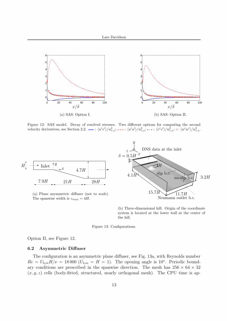
Figure 12 gives the maximum of the resolved stresses vs. x. Options I and II forcomputing the second velocity derivatives in U ′′ (see Section 2.2) are compared. OptionII uses only every second node, and hence U ′′ becomes larger (PSAS smaller) than withOption I. As a result, the turbulent viscosity is smaller with Option I as compared withOption II, and this explains why the resolved stresses are larger with Option I than with
12
Lars Davidson
0 20 40 60 80 100
0
1
2
3
4
5
6
PSfrag replacements
x/δ
(a) SAS: Option I.
0 20 40 60 80 100
0
1
2
3
4
5
6
PSfrag replacements
x/δ
(b) SAS: Option II.
Figure 12: SAS model. Decay of resolved stresses. Two different options for computing the secondvelocity derivatives, see Section 2.2. : 〈u′v′〉/u2
τ,x; : 〈u′u′〉/u2τ,x; : 〈v′v′〉/u2
τ,x; ◦: 〈w′w′〉/u2τ,x.
PSfrag replacements
21H
H4.7H
7.9H 28H
Inlet xy
(a) Plane asymmetric diffuser (not to scale).The spanwise width is zmax = 4H .
PSfrag replacements
DNS data at the inlet
Neumann outlet b.c.
no-slip b.c.slip b.c.
H
δ = 0.5H
4.1H
15.7H 11.7H
3.2H
x
y
z
(b) Three-dimensional hill. Origin of the coordinatesystem is located at the lower wall at the center ofthe hill.
Figure 13: Configurations.
Option II, see Figure 12.
6.2 Asymmetric Diffuser
The configuration is an asymmetric plane diffuser, see Fig. 13a, with Reynolds numberRe = Ub,inH/ν = 18 000 (Ub,in = H = 1). The opening angle is 10o. Periodic bound-ary conditions are prescribed in the spanwise direction. The mesh has 256 × 64 × 32(x, y, z) cells (body-fitted, structured, nearly orthogonal mesh). The CPU time is ap-
13
Lars Davidson
PSfrag replacements
x = 3H 6 14 17 20 24HPSfrag replacements
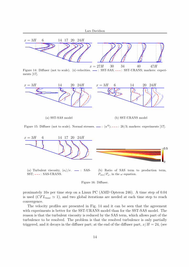
x = 27H 30 34 40 47HFigure 14: Diffuser (not to scale). 〈u〉-velocities. : SST-SAS; : SST-URANS; markers: experi-ments [17].
PSfrag replacements
x = 3H
6
14
17
20 24H
(a) SST-SAS model
PSfrag replacements
x = 3H 6 14
17
20 24H
(b) SST-URANS model
Figure 15: Diffuser (not to scale). Normal stresses. : 〈u′2〉; : 2k/3; markers: experiments [17].
PSfrag replacements
x = 3H 6 14 17 20 24H
(a) Turbulent viscosity, 〈νt〉/ν. : SAS-SST; : SAS-URANS.
0
0.5
(b) Ratio of SAS term to production term,Psas/Pω, in the ω equation.
Figure 16: Diffuser.
proximately 10s per time step on a Linux PC (AMD Opteron 246). A time step of 0.04is used (CFLmax ' 1), and two global iterations are needed at each time step to reachconvergence.
The velocity profiles are presented in Fig. 14 and it can be seen that the agreementwith experiments is better for the SST-URANS model than for the SST-SAS model. Thereason is that the turbulent viscosity is reduced by the SAS term, which allows part of theturbulence to be resolved. The problem is that the resolved turbulence is only partiallytriggered, and it decays in the diffuser part; at the end of the diffuser part, x/H = 24, (see
14
Lars Davidson
−2 −1 0 1 20
0.5
1
1.5
2
2.5
3
PSfrag replacements
x
y
(a) Zoom of the grid. Every second gridlines is shown.
(b) Experiments
X
Y
-1 0 1 2 3 4
0
1
2
3
4
5
PSfrag replacements
xy
(c) SST-SAS model
X
Y
-1 0 1 2 3 4
0
1
2
3
4
5
PSfrag replacements
x
(d) SST-URANS model
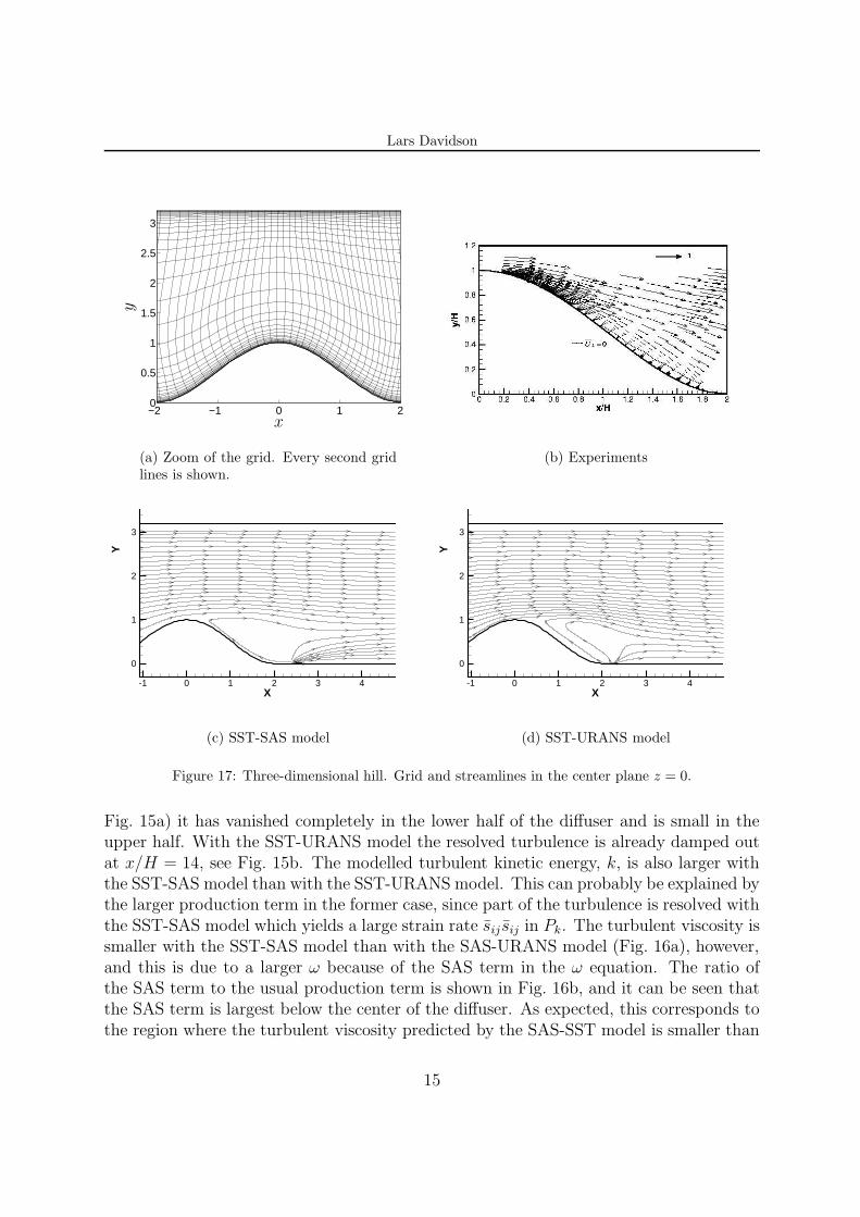
Figure 17: Three-dimensional hill. Grid and streamlines in the center plane z = 0.
Fig. 15a) it has vanished completely in the lower half of the diffuser and is small in theupper half. With the SST-URANS model the resolved turbulence is already damped outat x/H = 14, see Fig. 15b. The modelled turbulent kinetic energy, k, is also larger withthe SST-SAS model than with the SST-URANS model. This can probably be explained bythe larger production term in the former case, since part of the turbulence is resolved withthe SST-SAS model which yields a large strain rate sij sij in Pk. The turbulent viscosity issmaller with the SST-SAS model than with the SAS-URANS model (Fig. 16a), however,and this is due to a larger ω because of the SAS term in the ω equation. The ratio ofthe SAS term to the usual production term is shown in Fig. 16b, and it can be seen thatthe SAS term is largest below the center of the diffuser. As expected, this corresponds tothe region where the turbulent viscosity predicted by the SAS-SST model is smaller than
15
Lars Davidson
(a) SST-SAS model. (b) SST-URANS model.
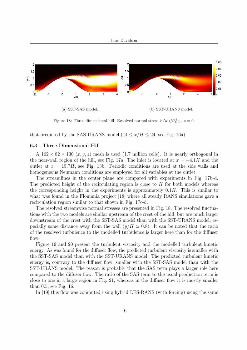
Figure 18: Three-dimensional hill. Resolved normal stress 〈u′u′〉/U2b,in. z = 0.
that predicted by the SAS-URANS model (14 ≤ x/H ≤ 24, see Fig. 16a)
6.3 Three-Dimensional Hill
A 162 × 82 × 130 (x, y, z) mesh is used (1.7 million cells). It is nearly orthogonal inthe near-wall region of the hill, see Fig. 17a. The inlet is located at x = −4.1H and theoutlet at x = 15.7H, see Fig. 13b. Periodic conditions are used at the side walls andhomogeneous Neumann conditions are employed for all variables at the outlet.
The streamlines in the center plane are compared with experiments in Fig. 17b-d.The predicted height of the recirculating region is close to H for both models whereasthe corresponding height in the experiments is approximately 0.1H. This is similar towhat was found in the Flomania project [18] where all steady RANS simulations gave arecirculation region similar to that shown in Fig. 17c-d.
The resolved streamwise normal stresses are presented in Fig. 18. The resolved fluctua-tions with the two models are similar upstream of the crest of the hill, but are much largerdownstream of the crest with the SST-SAS model than with the SST-URANS model, es-pecially some distance away from the wall (y/H ' 0.8). It can be noted that the ratioof the resolved turbulence to the modelled turbulence is larger here than for the diffuserflow.
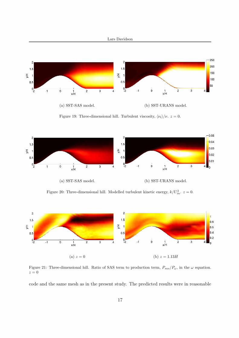
Figure 19 and 20 present the turbulent viscosity and the modelled turbulent kineticenergy. As was found for the diffuser flow, the predicted turbulent viscosity is smaller withthe SST-SAS model than with the SST-URANS model. The predicted turbulent kineticenergy is, contrary to the diffuser flow, smaller with the SST-SAS model than with theSST-URANS model. The reason is probably that the SAS term plays a larger role herecompared to the diffuser flow. The ratio of the SAS term to the usual production term isclose to one in a large region in Fig. 21, whereas in the diffuser flow it is mostly smallerthan 0.5, see Fig. 16.
In [19] this flow was computed using hybrid LES-RANS (with forcing) using the same
16
Lars Davidson
(a) SST-SAS model. (b) SST-URANS model.
Figure 19: Three-dimensional hill. Turbulent viscosity, 〈νt〉/ν. z = 0.
(a) SST-SAS model. (b) SST-URANS model.
Figure 20: Three-dimensional hill. Modelled turbulent kinetic energy, k/U 2in. z = 0.
(a) z = 0 (b) z = 1.13H
Figure 21: Three-dimensional hill. Ratio of SAS term to production term, Psas/Pω, in the ω equation.z = 0
code and the same mesh as in the present study. The predicted results were in reasonable
17
Lars Davidson
(a) Resolved normal stress 〈u′u′〉/U2b,in. (b) Turbulent viscosity, 〈νt〉/ν.
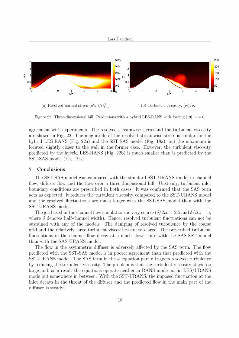
Figure 22: Three-dimensional hill. Predictions with a hybrid LES-RANS with forcing [19]. z = 0.
agreement with experiments. The resolved streamwise stress and the turbulent viscosityare shown in Fig. 22. The magnitude of the resolved streamwise stress is similar for thehybrid LES-RANS (Fig. 22a) and the SST-SAS model (Fig. 18a), but the maximum islocated slightly closer to the wall in the former case. However, the turbulent viscositypredicted by the hybrid LES-RANS (Fig. 22b) is much smaller than is predicted by theSST-SAS model (Fig. 19a).
7 Conclusions
The SST-SAS model was compared with the standard SST-URANS model in channelflow, diffuser flow and the flow over a three-dimensional hill. Unsteady, turbulent inletboundary conditions are prescribed in both cases. It was confirmed that the SAS termacts as expected: it reduces the turbulent viscosity compared to the SST-URANS modeland the resolved fluctuations are much larger with the SST-SAS model than with theSST-URANS model.
The grid used in the channel flow simulations is very coarse (δ/∆x = 2.5 and δ/∆z = 5,where δ denotes half-channel width). Hence, resolved turbulent fluctuations can not besustained with any of the models. The damping of resolved turbulence by the coarsegrid and the relatively large turbulent viscosities are too large. The prescribed turbulentfluctuations in the channel flow decay at a much slower rate with the SAS-SST modelthan with the SAS-URANS model.
The flow in the asymmetric diffuser is adversely affected by the SAS term. The flowpredicted with the SST-SAS model is in poorer agreement than that predicted with theSST-URANS model. The SAS term in the ω equation partly triggers resolved turbulenceby reducing the turbulent viscosity. The problem is that the turbulent viscosity stays toolarge and, as a result the equations operate neither in RANS mode nor in LES/URANSmode but somewhere in between. With the SST-URANS, the imposed fluctuation at theinlet decays in the throat of the diffuser and the predicted flow in the main part of thediffuser is steady.
18
Lars Davidson
The flow around the axi-symmetric hill is poorly predicted by both models. Thepredicted recirculating region in the center plane is much too large compared with experi-ments. On the lee-side of the hill a rather large unsteadiness prevails in both models, butthe resolved fluctuations are larger with the SST-SAS model than with the SST-URANSmodel. However, when compared with hybrid LES-RANS – which does give a flow fieldin reasonable agreement with experiments – the turbulent viscosity predicted with thetwo models is much too large.
The SAS term is expressed as the ratio of the von Karman length scale, Lvk,3D, to
the usual RANS turbulent length scale, c−1/4µ k1/2/ω. The von Karman length scale is
evaluated using data from a DNS simulation and from a hybrid LES-RANS simulation.It is found that when the DNS data are used the von Karman length scale expressed ininstantaneous velocity gradients closely follows the smallest grid spacing, i.e. the wall-normal spacing, ∆y. When the hybrid LES-RANS data are used the von Karman lengthscale in the wall region (i.e. the URANS region) is slightly larger than ∆y because ofrather larger turbulent viscosities, which make the smallest, resolved scales larger.
The concept of using the von Karman turbulent length scale for detecting unsteadinessis very interesting. This idea should be pursued further and could be used in connectionwith other models. In the SST-SAS model the von Karman length scale is used to triggeran additional source term. As an alternative it could probably also be used to change thevalue of a coefficient in a transport turbulence model.
REFERENCES
[1] R. Franke and W. Rodi. Calculation of vortex shedding past square cylinders with variousturbulence models, 8th turbulent shear flow. In 8th Symp. on Turbulent Shear Flows, pages20:1:1 – 20:1:6, Munich, 1991.
[2] G. Bosch and W. Rodi. Simulation of vortex shedding past a square cylinder with differentturbulence models. International Journal for Numerical Methods in Fluids, 28(4):601–616,1998.
[3] S. Johansson, L. Davidson, and E. Olsson. Numerical simulation of vortex shedding pasttriangular cylinders at high Reynolds number. Int. J. Numer. Meth. Fluids, 16:859–878,1993.
[4] P.R. Spalart, W.-H. Jou, M. Strelets, and S.R. Allmaras. Comments on the feasabilityof LES for wings and on a hybrid RANS/LES approach. In C. Liu and Z. Liu, editors,Advances in LES/DNS, First Int. conf. on DNS/LES, Louisiana Tech University, 1997.Greyden Press.
[5] A. Travin, M. Shur, M. Strelets, and P. Spalart. Detached-eddy simulations past a circularcylinder. Flow Turbulence and Combustion, 63(1/4):293–313, 2000.
[6] F.R. Menter, M. Kuntz, and R. Bender. A scale-adaptive simulation model for turbulentflow prediction. AIAA paper 2003–0767, Reno, NV, 2003.
[7] F.R. Menter and Y. Egorov. Revisiting the turbulent length scale equation. In IUTAMSymposium: One Hundred Years of Boundary Layer Research, Gottingen, 2004.
19
Lars Davidson
[8] F.R. Menter and Y. Egorov. A scale-adaptive simulation model using two-equation models.AIAA paper 2005–1095, Reno, NV, 2005.
[9] J.C. Rotta. Turbulente Stromungen. Teubner Verlag, Stuttgart, 1972.
[10] L. Davidson and S. Dahlstrom. Hybrid LES-RANS: An approach to make LES applicable athigh Reynolds number. International Journal of Computational Fluid Dynamics, 19(6):415–427, 2005.
[11] L. Davidson and S.-H. Peng. Hybrid LES-RANS: A one-equation SGS model combinedwith a k − ω model for predicting recirculating flows. International Journal for NumericalMethods in Fluids, 43:1003–1018, 2003.
[12] P. Emvin. The Full Multigrid Method Applied to Turbulent Flow in Ventilated EnclosuresUsing Structured and Unstructured Grids. PhD thesis, Dept. of Thermo and Fluid Dynam-ics, Chalmers University of Technology, Goteborg, 1997.
[13] M. Billson. Computational Techniques for Turbulence Generated Noise. PhD thesis, Dept.of Thermo and Fluid Dynamics, Chalmers University of Technology, Goteborg, Sweden,2004.
[14] L. Davidson and M. Billson. Hybrid LES/RANS using synthesized turbulence for forcingat the interface (in print). International Journal of Heat and Fluid Flow, 2006.
[15] M. Billson, L.-E. Eriksson, and L. Davidson. Jet noise prediction using stochastic turbulencemodeling. AIAA paper 2003-3282, 9th AIAA/CEAS Aeroacoustics Conference, 2003.
[16] L. Davidson. Hybrid LES-RANS: Inlet boundary conditions. In 3rd National Conferenceon Computational Mechanics – MekIT’05 (invited paper), Trondheim, Norway, 2005.
[17] C.U. Buice and J.K. Eaton. Experimental investigation of flow through an asymmetricplane diffuser. Report No. TSD-107, Thermosciences Division, Department of MechanicalEngineering, Stanford University, Stanford, California 94305, 1997.
[18] W. Haase, B. Aupoix, U. Bunge, and D. Schwamborn, editors. FLOMANIA: Flow-PhysicsModelling – An Integrated Approach, volume 94 of Notes on Numerical Fluid Mechanicsand Multidisciplinary Design. Springer, 2006.
[19] L. Davidson and S. Dahlstrom. Hybrid LES-RANS: Computation of the flow around a three-dimensional hill. In W. Rodi and M. Mulas, editors, Engineering Turbulence Modelling andMeasurements 6, pages 319–328. Elsevier, 2005.
20