Embed Size (px)
Citation preview

1
Evaluation of the Public Transportation System in Kabul by Time of Day User Equilibrium
Assignment
Mohammad Jalil EBRAHIMI
Associate Professor Kazushi SANO (Chairperson)
Assistant Professor Hiroaki NISHIUCHI
Department of Civil and Environmental System Engineering
Nagaoka University of Technology
Japan
March, 2015
Abstract: Public transportation is a relatively
high-capacity and energy-efficient alternative for
urban passenger transportation. With the
developing of society and economy, demand for
public transportation increased dramatically in
Kabul city. This paper probed into the public
transportation system in Kabul and evaluated its
development. Based on current situation and trend
in public transportation, the strategy scenarios for
public transportation development pointed out. In
each scenario discusses the effects of implementing
Bus Rapid Transit (BRT) in Kabul city, including
how to evaluate the systems and model bus
operations with current public transport situation in
the study area. For this purpose, the study fist
considering on traffic demand forecasting based on
four steps model, and make a Time of Day User
Equilibrium Assignment. Then, predict the future
demand to clarify the traffic condition in 2025 and
with regard to future traffic conditions that results
obtained from Time of Day User Equilibrium
Assignment, focused on strategy scenarios to
evaluate the system. Finally, in this research
focused on Cost-Benefit Analysis for introduction
of BRT system in Kabul city. And cost-benefit
analysis considered for a relatively long period, 30
years. During the construction of the project, its
cost is too high comparing to the benefit, but the
benefits during the years of service will dramatic
increased. It is intended that the buses should be
replaced by every 10 years, therefore the costs for
the new vehicle considered during the project
years. And also the operation cost considered
during the project life.
1. Introduction
In general, two strategies can improve the
transportation system and reduce the traffic
congestion: the expansion and the improvement of
the existing transportation infrastructures. In this
research efforts are made to focus more on the
second case, because it is suitable to the developing
cities which are unable to pay the high capital cost
of new construction. In the process of improving
the existing infrastructure it is necessary to improve
the public transportation system. Researches in this
field show that Bus Rapid Transit (BRT) system is
economical at high passenger density which is
compared with ordinary bus transit and other
automobiles. BRT system introduced based on
three scenarios. Therefore, the BRT should be
established linking the existing Kabul city, and also
the BRT network should cover some part of the
existing urban area as well. Feeder services from
the BRT stations should cover the entire city area
effectively. Terminals for inter-city bus services
should be located in the suburbs, and linked to the
city center by BRT or feeder services.
2. Objective of the study
Regarding this study, the main objectives of the
study are summarized in the following:
To forecast traffic demand, 2025 in Kabul city
by using Time of Day User Equilibrium
Assignment.
To find the best public transportation system
for Kabul city.
3. Study area and used data
Period planning to forecast will be considered 10
years. Focused area for the study comprises on
Kabul the capital of Afghanistan which is 275
square kilometers and around 5 million populations.
The data which are used in this research like
personal trip survey conducted by JICA, survey
questioner which is around 12,000 samples.
Preparation of zone base data base so, there are 22
zone in Kabul city, the zonal attributes like zoning
area size, population of each zone and employment
at workplace. Preparation of network data base
therefore route network including number of links,
number of nodes, links capacities and link flow.
Present and future socioeconomic data, travel time

2
by mode and fare of each mode, dwell time and
waiting time at bus stop.
4. Traffic Demand Forecast
4.1 Trip Generation/Attraction Model
Uses socioeconomic data to determine the number
of trips produced by traffic analysis zone, the
socioeconomic data normally includes population,
employment at workplace. To estimate this step of
the model use linear function:
…… (1)
Where zoning area size , population of each
zone, and is employment at
workplace. Are the parameters and b
is constant.
4.2 Trip Distribution Model
Trip distribution model determines where the trips
will go. This normally uses a gravity model to
estimate the trip distribution model, as follows:
(2)
Where is attracted trip in zone i, generated
trip from zone j and “d” is the distance between
zones.
4.3 Model Split Model
This step model determines what vehicles trips will
utilize when going from one zone to another.
Utility function and proportion function are
following:
(3)
(4)
Where is utility from zone i to j by mode k,
is cost from zone i to j by mode k, travel time
from zone i to j by mode k, and
are the
waiting and dwell time.
Figure 1 Actual proportion in 2008
Figure 2 Estimated proportions, 2088
4.4 Time of Day User Equilibrium Assignment
The model assumes the following two hypotheses:
1) The time duration is less than the maximum
travel time.
2) The traffic is uniformly generated and
distributed within each time durations
The presence of residual traffic that is left over to
the next time duration is handled by the OD traffic
adjustment for the next time duration. The main
functions which are used in time of day user
equilibrium assignment as follows;
5.4.1 Residual Traffic
Suppose that stands for the traffic that is
statically distributed onto the route k for the OD
pair rs during the time duration. Suppose also
that stands for the length of time duration and
for the travel time needed to reach the
ending node of the link from the origin node of
the route k. of the traffic generated on the
route k during the time duration, (j) is its
residual traffic that fails to pass the starting node of
the link j within that time duration. This residual
traffic is obtained by the following equation:
Where is the traffic that is statically
distributed onto route k for OD pair rs, during
the . And stands for the length of time
duration, is travel time the ending of node
of the link from origin node of the route k.
5.4.2 Adjustment traffic
The adjusted traffic includes the residual traffic
from the previous time duration can be obtained
from the following equation;
(6)
The model assumes the uniform traffic generation
and distribution per time duration for assignment.
Therefore, the time needed to reach the destination
on a given route is equal to the travel time on the
minimum path searched per OD pair. Supposing
that stands for the total traffic per OD pair per
time duration, the aggregate total of residual traffic
walk 39%
bike 8%
mic.bus
18% min.b
us 6%
L.bus 14%
taxi 12%
car 3%
Figure 1
walk 33%
bike 10%
mic.bus
19%
min.bus 7%
L.bus 16%
taxi 12%
car 3%
Figure 2

3
on all available routes is defined by the following
equation.
(7)
Where is for the total traffic OD pair per time
duration route network k zone r to s and is the
travel time on the minimum path searched per OD
pair. And also the traffic after residual traffic
adjustment can be obtained by the following
equation;
(8)
Furthermore, the OD traffic after residual traffic
adjustment can be expressed in the following
equation, by using the minimum path travel time.
(9)
5.4.3 Link Cost Function
To calculate the velocity of travel relative to traffic
congestion, can select one of three alternative link
cost functions (QV, BPR and DAVIDSON)
formulas, and define parameters for up to 99 QV
types from these formulas. Therefore in case of
time of day user equilibrium assignment considered
on BBR formula as follows;
(10)
By using STRADA program. Therefore, the
required input data as follow;
• OD Matrix by time of day (from 5am to 9pm), so
the time duration is every two hours and the
number of time durations is eight.
Figure 3 Distribution of Trip
• Network data & assignment parameter. The
number of links are 670, number of nodes are
464, number of zones are 74 and number of
modes are seven.
5.4.4 Outputs of Route Related Data
The STRADA Time of Day User Equilibrium
Assignment is calculate to output unique link
flows, but this does not necessarily mean that it
offers similarly unique route-related data outputs.
The assignment does perform the minimum route
search for loading as indicated in the algorithms
already explained above. This can be put to use to
obtain the approximate route-related data. Three
route-related data outputs, namely, link OD details,
directional link flows and route information are
saved up during the iterated loadings. The result
shown in the following figure;
Thus according to the result it is clear that area
under the study (Kabul city) there is traffic
congestion and this problem is different at during
time of the day. Given the current state of the
Kabul city, the congestion caused by rapid
population growth, lack of public transport
services, increasing the number of passenger cars
and blocking roads because of the security
problems, and other researches that have been done
already shows that the main problems, namely in
the public transportation services are low.
Therefore, the strengthening of the public
transportation can reduces the congestion and
travel time from origin to destination. To reduce
this problem (traffic congestion), the solutions
ways must be addressed, which is satisfaction of
the people, be efficient and useful. Thus, the
policies that meet the expectations of a number of
scenarios were considered to be closer to the
target. The obtained results from Time of Day User
Equilibrium Assignment (TDUEA) are shows in
Figures 2. The results show that there is traffic
congestion in Kabul city and it is clear that the
congestion is different during the time of the day
especially at peak hours and off-hours (5-7am and
7-9 pm). The color in the figures displays the link
congestion levels. The congestion is expressed by
the total traffic volume divided by the link
capacity. For example, the red colors means that
0
200,000
400,000
600,000
800,000
1,000,000
1,200,000
No. o
f T
rip
77
24
24
54
1010
1413
9
10
10
8
12
7
6
24
19
14
14
818
118
1817
18
17
2020
1718
8
713
13
17 5
22
1
1 2
2
3
4
56 3
1 4
4
32
45
44
89
11
0
1
77
9
977
13
8
27
30
6
6
1
1
7
77
7
5 5
7
7
8
8
1414
1818
4
4
5 5
18
19
4
4
18
18
66
9
9
17
14
16
16
2
2
5
6
9
9
12
226
611
12
215
18
12
21
1216
1312
28
32
10
23
12
13
1416
66
4
4
13
78
9
9
5
5
4
4
6
6
12
11
1416
1
7
12
15 10
10
5
6
55
2324 1
14
4 88
58
56
15
14
19
20
11
12
1112
8 10
26
26
514
5
18
78
31
33
4
48
7
3
3
11
12
20
18
66
5
55
526
26
4
4
8
9
1
1
60
60
24
23
1212
26
11
28
7
19
414
2
23
25
16
17
20
21
18
19
1511
1410
18
18
1211
13
15
9
9
18
19
9
9
1
1
22
54
5 5
0
0
21
21
20
14
1616
22
11
2
3
3
2
1
1
1913
2012 14
5
517
12
12
9
9
1010
20
16
11
32
23
2
2
2
2
44
2
2
3
2
3
3
0
0
0
0
9 11
3 3
3
3
33
33
33
13
14
0
00
0
0
0
1414
14
14
14
14
1414
16
16
9 666
6
66
6
6 6
0
0
0
0
0
00
00
0
11
12
5
4
8
9
17
22
24
26
22
23
10
10
15
14
18
20
19
21
3333
45
21
21
7
313
13
7
7
5
5
16
17
8
50
7 8001
1
2
1
3 3
24
18
1718
17
18
56
44
18
1911
12
32
13
13
87
1
1
7
7
00
00
0
0
22
2
2
0
0
2
3
2
3
2
3
20
16
20
16
16
20
6 6
17
15
11
11
17
15
41
42
9
6
96
2
2
1 1
1
11
1
5 55 5
3 3
22
7
720
20
6
6
4 5
2
2
1 1
60
60
60
60
5
511
13
2
3
22
531
2
96
1514
13
13
8
7
4
5
5
5
12
10 28
2641
3724
18
24
18 21
1121
11
68
0
0
8
7
8
7
9
9
5
5
12
14
10
9
10
10
686
8
2212
5952
73 50
52
00
12
1 2
13
15
1 2
53
51
0
1
8
10 3
3
78
87
98
33
2
2
22
29
2629
2619
13
22 16
19
13
1119
18
2225
2124
11
44
23
1514 14
13 1716
7
82
2
3
210
9
1
1
2
2
33
30
31
30
31 1012
6
6
13
11
88
18
19
8
9
2
2
4
3
8
7
22
45
551112
18
18
2
2
7
7
12
1218
1914
14
23
23
11
11
11
2323
00
0
0
4
4
2
2
1
1
11
11
5
5
11
9
119
14
13
1413
1110
2019
13
13 7
7
13
13
20
16
3
318
18
23
16
23
16
23
16
26
32
201
6
201
6
6
61011
9
109
1017
19
1617
19
18
1110
11
10
11
1011
10
1110
10
10
1010
17
17 17
17
20
19
0
0
0
0
18
14
4543
45
43
731717
00
1915
1315
21
27
17
17
17
17
33
31
1
1
23
3223
3223
32
23
32
23
32
66
18
19
1918
1
1
11
55
13
13
32
30
31
33
0
0
29
30
29
3014
13
44
25
21 9
9
17
16
0
25
25
25
25
35
36 9
99
9
37
37
49
50
25
25
38
38
30
31
22
19
2219
1413
6
6
6
610
10
12
13
5
5
55
1010
12
13
0
0
0
4
44 4
14
14
18
1831
31
20
19
6
6
1111
16
16
10
10
21
23
5
5
872222
1514
77
101
0
44
1920
7
7
10
0
1
11
11
17
15
31
31
13
14
11
13
13
3 3
1
1
0
0
5
6
21
2
1
1312
10
10
1
2
21
2110
9
18
14
9
9
50
52
0 00 0
2111
2
1
42
46
34
36
3
2
30
29
13
13
242
0
19
1727
23
2625
55
14
14
22
23
25
25
12
12
88
22
10
10
1010
0
0
11
11
11
18
23
11
11
12
21
20
11
11
109
10
10
66 4
5
10
10
5
55
5
10
10
77
7
77
7
7 766
11
44
6
6 55
5
5
6
64
4
1
1 9
9
7
7
2
2
3 3
7
7
15
15
4
4
10
10
9
9
9
9
10
10
1212 7
7
7712
12
15
16
1616
16
16
99 6
6
661010
22
23
2323
23
23
23
23
23
23
39
39
40
40
40
40
89
31
31
20
17
33
17
15
5
5
19
15
4
5
1513
8
7
1010
5
5
13
13
2
2
4
411
11
1010
55
1920
7
7 12
13
1515
4
5
87
49
53
11
12
8
8
606
4
26
26
2626
2626
15
14
13
12
3 3 2321
2321
222
1
14
16
20
19
34
35
34
35
21
21
22
23
23
23
23
12
12
13
12
18
179
8
7
7
21
20
13
13
117
1
1
15
15
2121
0 0
5
5
1724
7
14 15
15
21
28
LEGEND :
Traffic Flow
( Mode: + 1 + 2 + 3 + 4 + 5 + 6 + 7 )
VCR<1.00
VCR<1.20
VCR<1.50
1.50<VCR
scale: 1mm =3000(pcu)
Result from TDUEA
Figure 4: Traffic Flow in peak-hours (7:00 – 9:00) in 2008
)(1)(0
Cx
txta
a
aaa
4
the VCR>1.5, the blue colors shows that the VCR<
1 and the green color shows that the VCR<1.2.
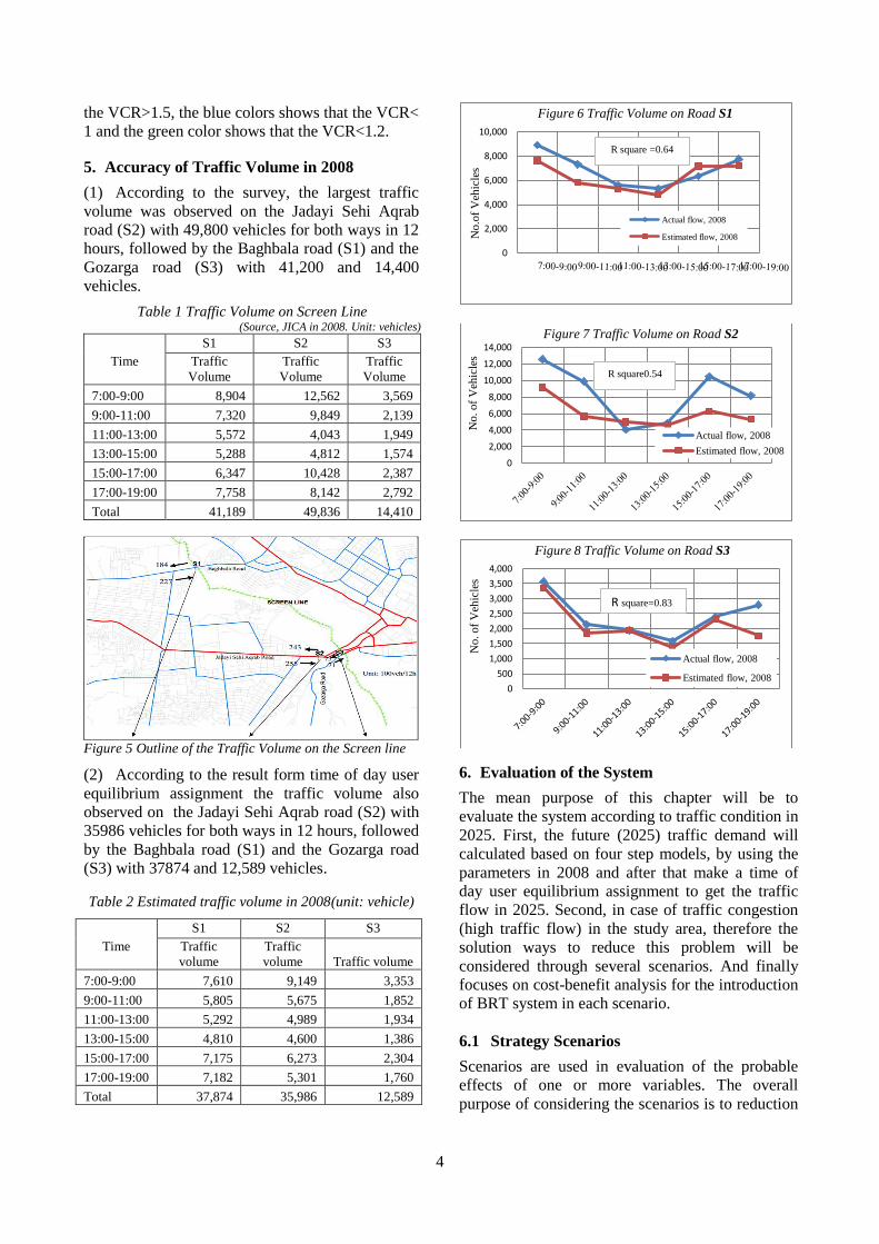
5. Accuracy of Traffic Volume in 2008
(1) According to the survey, the largest traffic
volume was observed on the Jadayi Sehi Aqrab
road (S2) with 49,800 vehicles for both ways in 12
hours, followed by the Baghbala road (S1) and the
Gozarga road (S3) with 41,200 and 14,400
vehicles.
Table 1 Traffic Volume on Screen Line (Source, JICA in 2008. Unit: vehicles)
Time
S1 S2 S3
Traffic
Volume
Traffic
Volume
Traffic
Volume
7:00-9:00 8,904 12,562 3,569
9:00-11:00 7,320 9,849 2,139
11:00-13:00 5,572 4,043 1,949
13:00-15:00 5,288 4,812 1,574
15:00-17:00 6,347 10,428 2,387
17:00-19:00 7,758 8,142 2,792
Total 41,189 49,836 14,410
Figure 5 Outline of the Traffic Volume on the Screen line
(2) According to the result form time of day user
equilibrium assignment the traffic volume also
observed on the Jadayi Sehi Aqrab road (S2) with
35986 vehicles for both ways in 12 hours, followed
by the Baghbala road (S1) and the Gozarga road
(S3) with 37874 and 12,589 vehicles.
Table 2 Estimated traffic volume in 2008(unit: vehicle)
6. Evaluation of the System
The mean purpose of this chapter will be to
evaluate the system according to traffic condition in
2025. First, the future (2025) traffic demand will
calculated based on four step models, by using the
parameters in 2008 and after that make a time of
day user equilibrium assignment to get the traffic
flow in 2025. Second, in case of traffic congestion
(high traffic flow) in the study area, therefore the
solution ways to reduce this problem will be
considered through several scenarios. And finally
focuses on cost-benefit analysis for the introduction
of BRT system in each scenario.
6.1 Strategy Scenarios
Scenarios are used in evaluation of the probable
effects of one or more variables. The overall
purpose of considering the scenarios is to reduction
0
2,000
4,000
6,000
8,000
10,000
No.o
f V
ehic
les
Figure 6 Traffic Volume on Road S1
Actual flow, 2008
Estimated flow, 2008
R square =0.64
0
2,000
4,000
6,000
8,000
10,000
12,000
14,000
No. of
Veh
icle
s
Figure 7 Traffic Volume on Road S2
Actual flow, 2008
Estimated flow, 2008
R square0.54
0
500
1,000
1,500
2,000
2,500
3,000
3,500
4,000
No. of
Veh
icle
s
Figure 8 Traffic Volume on Road S3
Actual flow, 2008
Estimated flow, 2008
R square=0.83
Time
S1 S2 S3
Traffic
volume
Traffic
volume Traffic volume
7:00-9:00 7,610 9,149 3,353
9:00-11:00 5,805 5,675 1,852
11:00-13:00 5,292 4,989 1,934
13:00-15:00 4,810 4,600 1,386
15:00-17:00 7,175 6,273 2,304
17:00-19:00 7,182 5,301 1,760
Total 37,874 35,986 12,589
5
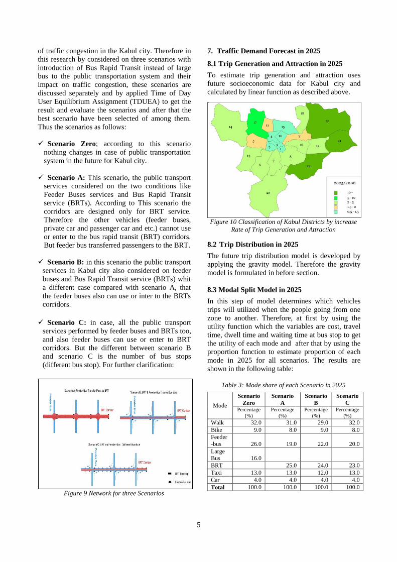
of traffic congestion in the Kabul city. Therefore in
this research by considered on three scenarios with
introduction of Bus Rapid Transit instead of large
bus to the public transportation system and their
impact on traffic congestion, these scenarios are
discussed separately and by applied Time of Day
User Equilibrium Assignment (TDUEA) to get the
result and evaluate the scenarios and after that the
best scenario have been selected of among them.
Thus the scenarios as follows:
Scenario Zero; according to this scenario
nothing changes in case of public transportation
system in the future for Kabul city.
Scenario A: This scenario, the public transport
services considered on the two conditions like
Feeder Buses services and Bus Rapid Transit
service (BRTs). According to This scenario the
corridors are designed only for BRT service.
Therefore the other vehicles (feeder buses,
private car and passenger car and etc.) cannot use
or enter to the bus rapid transit (BRT) corridors.
But feeder bus transferred passengers to the BRT.
Scenario B: in this scenario the public transport
services in Kabul city also considered on feeder
buses and Bus Rapid Transit service (BRTs) whit
a different case compared with scenario A, that
the feeder buses also can use or inter to the BRTs
corridors.
Scenario C: in case, all the public transport
services performed by feeder buses and BRTs too,
and also feeder buses can use or enter to BRT
corridors. But the different between scenario B
and scenario C is the number of bus stops
(different bus stop). For further clarification:
Figure 9 Network for three Scenarios
7. Traffic Demand Forecast in 2025
8.1 Trip Generation and Attraction in 2025
To estimate trip generation and attraction uses
future socioeconomic data for Kabul city and
calculated by linear function as described above.
Figure 10 Classification of Kabul Districts by increase
Rate of Trip Generation and Attraction
8.2 Trip Distribution in 2025
The future trip distribution model is developed by
applying the gravity model. Therefore the gravity
model is formulated in before section.
8.3 Modal Split Model in 2025
In this step of model determines which vehicles
trips will utilized when the people going from one
zone to another. Therefore, at first by using the
utility function which the variables are cost, travel
time, dwell time and waiting time at bus stop to get
the utility of each mode and after that by using the
proportion function to estimate proportion of each
mode in 2025 for all scenarios. The results are
shown in the following table:
Table 3: Mode share of each Scenario in 2025
Mode
Scenario
Zero
Scenario
A
Scenario
B
Scenario
C Percentage
(%)
Percentage
(%)
Percentage
(%)
Percentage
(%)
Walk 32.0 31.0 29.0 32.0
Bike 9.0 8.0 9.0 8.0
Feeder
-bus 26.0 19.0 22.0 20.0
Large
Bus 16.0
BRT 25.0 24.0 23.0
Taxi 13.0 13.0 12.0 13.0
Car 4.0 4.0 4.0 4.0
Total 100.0 100.0 100.0 100.0

6
8.4 Time of Day User Equilibrium Assignment
As mentioned above that the model assumes the
following two hypotheses like: (1) the time duration
is less than the maximum travel time; (2) the traffic
is uniformly generated and distributed within
duration of time. The OD matrix data must be
prepared per time duration, each file name
numbered seriallyfrom1 for the first time duration
through the last. After analyzing the results
achieved for all scenarios.
8.4.1 Result from Time of Day User Equilibrium
Assignment: The STRADA Time of Day User
Equilibrium Assignment is calculating to output
unique link flows shown in figure 5.10. The
assignment does perform the minimum route
search for loading as indicated in the algorithms
already explained above. This can be put to use to
obtain the approximate route-related data.
Three route-related data outputs, namely,
Link OD details,
Directional link flows
Route information
Figure 11 Traffic flow in off peak hours (5:00 to 7:00) in
2025
Figure 12 Traffic flow in peak-hours (7:00 to 9:00) in
2025
Figure 7 shows there is traffic congestion in Kabul
city and it is clear that the congestion is different
during the time of the day especially at peak hours
and off-hours (5-7am and 7-9 pm). The colors
displayed the level links congestion. The
congestion is expressed by the total traffic volume
divided by the link capacity. For example, the red
colors means that the VCR>1.5, the blue colors
shows that the VCR< 1 and the green color shows
that the VCR<1.2.
Table 4 Results from TDUEA for Scenarios
Evaluation
Indices Mode
Scenario
Zero
Scenario
A
Scenario
B
Scenario
C
Lar
ge-
Bus
&
Fee
der
-Bus
BR
T &
Fee
der
Bus
(Tra
nsf
er
pas
s. t
o B
RT
)
BR
T &
Fee
der
Bus
(sam
e B
us
stop)
BR
T &
Fee
der
Bus
(dif
fere
nt
Bus-
stop)
PCU-Km
Large-Bus 69,787
BRT 76,943 96,796 82,956
Feeder-Bus 142,962 178,902 196,792 183,336
PCU-hour
Large-Bus 2,972
BRT 1,843 1,708 1,612
Feeder-Bus 12,177 4,815 3,671 3,114
Total length
Large-Bus 190
BRT 190 190 190
Feeder-Bus 190 190 190 190
Average
VCR
Large-Bus 0.43
BRT 0.13 0.12 0.12
Feeder-Bus 0.68 0.32 0.23 0.22
Average
speed
Large-Bus 30.4
BRT 39.0 38.5 37
Feeder-Bus 34.6 37.0 38.5 36.4
9. Measure of Cost-Benefit Analysis: To
evaluation the CBA there is several measures to
compare benefits to cost in a cost benefit analysis.
Therefore, all benefits and costs over the project’s
lifecycle are discounted to present values and the
costs are subtracted from the benefits to obtain the
NPV, which must be a positive number for the
project to be justified. When multiple project
alternatives exist, the alternative with the largest
NPV of net benefits is typically the preferred
alternative, though sometimes, other factors
including project risks and funding availability may
play a role in the selection of an alternative with a
lower, positive NPV as follows:
(11)
And also the other measure to evaluate CBA
benefit cost ratio (BCR) which is a ratio where the
present value of benefits is divided by the present
value of the initial agency investment cost. When
benefits exceed costs, the ratio is greater than 1 and
11
2
22
6
13
11
14
1
8
22
12
148
813
18
13
89
16
4
1 3
7
41
2
0
41
0
1
0 12
712
7
19
5
1
4
46
4
11
11
14
3
4
20
4 9
13
9
13
5
4
3
7
15
4
0
9
1599
12
25
11
12
6
54
3
5
11
53
8
16
6
3
26 11
6
7
24 3
2
5
65
27
23
15
15
13
29
7
15
5
45
1111
4
10
27
5
77
25
5
13
3
58
25
14
1917
141728202423
9 8
21
15
9
15
20
15
6
4
2
7
0
17
14
15
2
1
1
3
1
17 18 7
16
14
7
6
12
3
14
0
0
1
0
1
5
0
0
8
2
2
2
2
2
11
1313
13
1314
10
16
1414
5
0 0 00
0
10
4
8
19 30
13
6
12
87
25
22
8
812
13 7
18
10
0
11
0
01
13
20 20
4
3
21
17
5
14101
7
0
0
1 1
1
12
12
12
8
24
21
12
52
10
10
6
1
11
7
7
10
58
8
3
2
0
58 58
4 5
3
3
21
10
27
14
10
67
6
18
2715
15
88
8
77
19
3
395448
9
9
99
1
8
5
2
2
9
1 4
0
13 1
6
1
1
2
1
1
18
18
10
414
12
19
30
311
5
5
11
10
10 7
2
0
6
0
1
1
2020
4
7
7
10
14
8 2 43
13
410
21
2
8
1125
21
1
1
1
0
0
25
5
51
1
0
7
8
8
9
9
7
17
5
14
13
15
32
10 10 10
25
12
12
79
0
11
10
11
7
7
77
7
15
15
6
6
14
5
51
03
5
12
7
7
21
3
1414
14
14
14
5
15
15
1
1
3
34
33
45
66
7
5
22
13
18
0
16
16
50
77
22
24
16
27 17
16
16
7
21
216
1
2
2
23
1
0
0
0
22
2
15
16
14
6
12 14
1
14
4
59
4
7
10
4
16
10
0
2
21
12
21
13
0
34
2
1
6
00
11
10
1
1754
5
15
8
8
1
1
8
2
6
12
20
1913
20
9
11
20
24
7
3
11
1
11
1
20
0
0
4
18
414
10
5
4
10
28
10
7 6
6
6
6
0
45
4
5
54
1 8
7
2
3
6
4
14
6
11
8
10
10 7
710
14
14
14
7 6
5
8
21
21
21
21
21
37
36
37
17
20
11
7
11
7
6
12
12
5
9
5
11
3
410
95
20
6 14
15
4
17
6
36
19
41
25
2425
13
11
3 19
19
19
14
17
30
31
21
1
23
22
11
11
159
6
18
9
8
1
17
17
15
10
15 11
25
LEGEND :
Traffic Flow
( Mode: + 1 + 2 + 3 + 4 + 5 + 6 + 7 )
VCR<1.00
VCR<1.20
VCR<1.50
1.50<VCR
scale: 1mm =2000(pcu)
40
46
47
48
58
47
63
5
30
77
38
4452
6049
93
49
3840
61
41
38 24
20
227
23
11
19
15
29
8
10
31
3531
36
40
37
3
29
2933
29
27
70
82
21
22
99
18 36
39
27
60
33
15
32
27
1013
21
3
31
643145
76
74
46
48
49
31
20
9
33
45
2215
32
68
49
23
78 20
24
23
74 23
27
32
23
893
71
50
49
38
104
47
64
21
166
3747
28
29
63
21
3838
96
18
60
23
235
81
51
4866
525298819177
63 35
46
50
50
90
99
90
22
15
49
42
4
43
48
48
16
3
11
11
4
60 91 47
61
51
35
55
38
41
80
25
13
31
4
4
53
46
46
34
46
46
30
3838
38
3846
33
44
44
44
21
4 4 44
4
29
9
24
69 111
76
48
35
4964
143
47
46
33
69
60 38
48
41
8
194
6
17
20
63
75 75
21
17
76
50
47
42424
18
16
16
11
11
11
15
17 17
17
38
32
78
59
83
186
33
33
21
8
269
38
42
12
9
1543
33
21
14
10
235 235
2848
15
15
24
14
33
93
42
42
2438
37
72
96
5858
6565
36
2
3131
99
23
637972
47
47
47
11
339
97
7
10
10
50
8 98
10
38 15
26
20
23
11
14
14
55
38
35
823
43
67
109
10415
23
10
28
18
33 28
11
4
20
1
13
14
9090
43
23
41
42
75
25 45 4233
234
24
4
46
19
31
3576
62
0
0
27
27
23
4
4
78
3
3
18
1813
5
11
38
53
53
59
59
43
97
30
46
40
57
1247
59 59 59
89
59
59
333
9
1919
78
24
38
43
43
4343
43
33
33
69
69
84
2
8
87
87
87
38
86
351
32
37
91
91
61
41
8080
80
80
80
29
58
58
17
39
79
139
166
0
0
85
90
4
53
32
75
43
48
8
100
100
222
36
368
148
10
0
111 80
136
136
53
85
4172
3
16
416
4135
3
8
8
8
54
54
55
29
28
84
22
46
48
32
82
18
30
63
37
18
26
12
47
39
12
11
59
83
81
40
7
79
18
9
16
24
11
21
27
26
9
4388
87
99
98
99
11
47
8
88
102
28
4
85
69
45
83
102
94
30
40
96
92
55
29
15
38
32
8
36
19
77
9
31
9
77
43
33
40
2416
40
1525
40
27 27
27
27
25
3
1820
17
21
20
18
6 31
28
10
14
24
33
38
26
46
31
41
45 26
3041
56
56
56
31
26
25
31
85
86
85
84
84
149
149
151
74
76
45
29
45
27
45
29
46
27
36
23
49
10
19
39
31
28
83
37 46
40
43
75
115
56
99
14
8
101
101102
57
35
22 8
0
80
78
46
83
127
129
67
24
95
94
44
47
6036
46
52
32
40
38
63
41
63
102
LEGEND :
Traffic Flow
( Mode: + 1 + 2 + 3 + 4 + 5 + 6 + 7 )
VCR<1.00
VCR<1.20
VCR<1.50
1.50<VCR
scale: 1mm =5000(pcu)

7
implies that the project is worth pursuing. The
BCA function as follows:
(12)
(13)
Where NPV is net present value, BCR is benefit-
cost ratio, b is benefit & c is cost, t is the period of
project life, r is discount rate and i is internal rate
of return (IRR)
9.1 Cost-Benefit Analysis for introduction of
BRTs: category of cost considered on capital cost,
operation and maintenance cost. And also category
of benefits considered on benefit to change in travel
time, benefit to change in vehicle operation cost for
driver and fare transit user, benefit to change in
emission of criteria pollutants and benefit to change
in crash costs.
Table 5 Scenarios Characteristic
Cost-benefit analysis consider for a relatively long
period, 30 years. The results show that during the
construction of the project, its cost is too high
comparing the benefit, but the benefits during the
years of service will dramatic increased. It is also
intended that the buses should be replaced by every
10 years, therefore the costs for the new vehicle
also considered during the project years. And the
operation cost in each year considered. For further
clarification of these issues, the following tables
are displayed.
Figure 13 Costs-benefits during project life, Scenario A
Figure 14 Costs-benefits during project life, Scenario B
Figure 15 Costs-benefits during project life, Scenario C
9.2 Evaluation of Scenarios:
Scenario A; in this scenario the pcu-km is
255,845, pcu-hour is 6,658 and average speed is
39 kilometer per hour, therefore this scenario
will provide a better service and more
appropriate compare to Scenario zero and other
scenarios, but according to the economic
indicators (cost-benefit analysis) this scenario is
much costly compare to the scenarios.
Scenario B; the pcu-km in this scenario is
293,588, pcu-hour is 5,379 and average speed is
38 kilometer per hour. Therefore this scenario
also will provide better services than scenario
zero and scenario C. And also according to
economic indicators (cost-benefit analysis)
Scenario B has low cost compared to scenario
A, and is the best choice.
Scenario C; the pcu-km is 286,292, pcu-hour is
4,726 and average speed is 36,4 kilometer per
hour. Therefore base on these indicators this
scenario cannot provide better service and more
appropriate than scenarios A&B. But, according
to the economic indicators (cost-benefit
analysis) the cost is low compared to other
scenarios like scenario A&B.
In detail according to CBA indices, Scenario B
represented a positive NPV with a highest net
benefits compare to scenario A and scenario C.
Similarly, scenario A and scenario C also has a
0
20,000,000
40,000,000
60,000,000
80,000,000
100,000,000
120,000,000
140,000,000
160,000,000
180,000,000
Cost Benefit
0
20,000,000
40,000,000
60,000,000
80,000,000
100,000,000
120,000,000
140,000,000
160,000,000 Cost Benefit
0
20,000,000
40,000,000
60,000,000
80,000,000
100,000,000
120,000,000
140,000,000
160,000,000
Cost Benefit
Scenario
zero
Scenario
A
Scenario
B
Scenario
C
Total No. of
passengers
2,463,872
2,594,402 2,774,298 2,524,392
Total corridors (km)
92 92 92
No. of station 92 92 153
No. vehicles
931 750 690
On-board fare
collection
931 750 690
Traffic signal
41 41 41
Passenger on board
Information
931 750 690
8
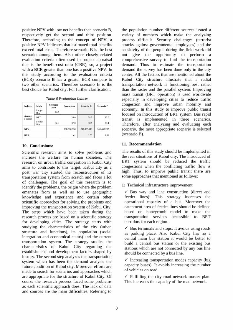
positive NPV with low net benefits than scenario B,
respectively get the second and third position.
Therefore, according to the concept of NPV, a
positive NPV indicates that estimated total benefits
exceed total costs. Therefore scenario B is the best
scenario among them. Also other closely related
evaluation criteria often used in project appraisal
that is the benefit-cost ratio (CBR), so, a project
with a BCR greater than one has a positive NPV. In
this study according to the evaluation criteria
(BCR) scenario B has a greater BCR compare to
two other scenarios. Therefore scenario B is the
best choice for Kabul city. For further clarification:
Table 6 Evaluation Indices
10. Conclusions:
Scientific research aims to solve problems and
increase the welfare for human societies. The
research on urban traffic congestion in Kabul City
aims to contribute to this target. Kabul city as a
post war city started the reconstruction of its
transportation system from scratch and faces a lot
of challenges. The goal of this research is to
identify the problems, the origin where the problem
emanates from as well as to use geographic
knowledge and experience and certain other
scientific approaches for solving the problems and
improving the transportation system of Kabul City.
The steps which have been taken during the
research process are based on a scientific strategy
for developing cities. The strategy starts with
studying the characteristics of the city (urban
structure and functions), its population (social
integration and economical status) and the current
transportation system. The strategy studies the
characteristics of Kabul City regarding the
establishment and development factors shaped by
history. The second step analyzes the transportation
system which has been the demand analysis the
future condition of Kabul city. Moreover efforts are
made to search for scenarios and approaches which
are appropriate for the structure of Kabul City. Of
course the research process faced some problems
as each scientific approach does. The lack of data
and sources are the main difficulties. Referring to
the population number different sources issued a
variety of numbers which make the analyzing
process difficult. Security challenges (terrorist
attacks against governmental employees) and the
sensitivity of the people during the field work did
not give the opportunity to perform a
comprehensive survey to find the transportation
demand. Thus to estimate the transportation
demand the survey has been done only in the city
center. All the factors that are mentioned about the
Kabul City structure illustrate that a radial
transportation network is functioning best rather
than the raster and the parallel system. Improving
mass transit (BRT operation) is used worldwide
especially in developing cities to reduce traffic
congestion and improve urban mobility and
economy. In this study to improve public transit
focused on introduction of BRT system. Bus rapid
transit is implemented in three scenarios.
Therefore, after analyzing and evaluating each
scenario, the most appropriate scenario is selected
(scenario B).
11. Recommendation
The results of this study should be implemented in
the real situations of Kabul city. The introduced of
BRT system should be reduced the traffic
congestions when the conflicting traffic flow is
high. Thus, to improve public transit there are
some approaches that mentioned as follows:
1) Technical infrastructure improvement
Bus way and lane construction (direct and
feeder lines): This strategy increases the
operational capacity of a bus. Moreover the
catchment area of feeder lines should be defined
based on honeycomb model to make the
transportation services accessible to BRT
corridors for each region.
Bus terminals and stops: It avoids using roads
as parking place. Also Kabul City has no a
central main bus station it would be better to
build a central bus station or the existing bus
stations which are not connected by any bus line
should be connected by a bus line.
Increasing transportation modes capacity (big
capacity buses): It avoids increasing the number
of vehicles on road.
Fulfilling the city road network master plan:
This increases the capacity of the road network.
Indices Mode Scenario
zero Scenario A Scenario B Scenario C
Averag
e speed
Large-
Bus 30.4
BRT 39.0 38.5 37.0
Feeder-
Bus 34.6 37.0 38.5 36.4
NPV 208,610,930 247,883,411 140,483,235
BCR 1.41 1.53 1.31

9
2) Administrative infrastructure improvements
Improvement of revenue collection process: it
supports the quality of operation and
maintenance, especially the fleet operation which
is performed by governmental public
transportation.
Commercialization of bus lines: the roads in
the city as the realms of the city can be profitable.
The bus lines should be leased to the private
sector but under the control and supervision of
the government. The government should control
the quality and accessibility of the private
companies which are operating on the bus line
and defined the link between transportation and
economic opportunities for the private sector.
REFERENCES
AUDA, A. &. (2005). Bus Rapid Transit system,
Ahmedabad. CETP University , 8-18.
Bartman, K. (2009). Transit System Evaluation
Process: From Planning to Realization. 7.
Bartman, K. (n.n.). Transit System Evaluation
Process: From Planning to Realization. 9.
Jffery Ang-Oslon, P. a. (April 2011). Cost-Benefit
analysis of converting a lane for Bus Rapid Transit
(BRT) - Phase 2 Evaluation and Methodology.
National coorperative highway research program ,
3.
Petersen, N. J. (1995). Benefit-cost analysis: a
State’s perspective. Exploring the Aplication of
Benefit-Cost Methodologies to Transportation
Infrastructure Decision-making. Washington:
FHWA.
Schwenk, J. C. (2002). Evaluation Guidelines for
Bus Rapid Transit Demonstration Projects.
Cambridge: Research and Special Programs
Administration .
Wright , L., & Hook, W. (2007). BRT Planning
Guide. New York: Institute for Transportation &
Development Policy.
Wright, 2. a. (2013). Issues Regarding Bus Rapid
Transit Introduction to Small and MediumSize
Cities of Developing Countries in East Asian
Region. 2-3.
Yasuhiro UJII, n. (n.n.). Development of Time of
Day User Equilibrium Traffic Assignment Model
Considering in Toll Load on Expressways. 5-6.
Yasuhiro, U. (n.n.). Develoment of Time-of-Day
User Equilibrium Traffic Assignment Model
Considering Toll load on Expressways. User
Equilibrium, Time-of-Day Traffic Assignment,
Expressway , 3-4.