EVALUATION OF THE PLUMB LINE CURVATURE EFFECT ON

THE DEFLECTION OF THE VERTICAL

HUNG PEN-SHAN

January 1986

TECHNICAL REPORT NO. 121

PREFACE

In order to make our extensive series of technical reports more readily available, we have scanned the old master copies and produced electronic versions in Portable Document Format. The quality of the images varies depending on the quality of the originals. The images have not been converted to searchable text.

EVALUATION OF THE PLUMB LINE CURVATURE EFFECT ON THE

DEFLECTIONS OF THE VERTICAL

Hung Pen-shan

This report is an unaltered printing of the author's Master of Science in Engineering thesis

submitted to this department in October 1985

Department of Geodesy and Geomatics Engineering University of New Brunswick

P.O. Box 4400 Fredericton, N .B.

Canada E3B 5A3

January 1986 Latest Reprinting February 1994

ABSTRACT

The curvature of the plumb line should be considered

1n order to find the undistorted geodetic networks without

the plumb I ine curvature effect and to determine the astro-

geodetic geoid as we I I as for other purposes. A few

approaches have been developed to estimate the curvature

effect. In most of the methods, the need for sufficient

gravity data, the knowledge of the density distribution, and

other data make the estimation of the plumb line curvature

effect a difficult task.

Without knowing the density distribution inside the

earth, the curvature effect can be determined from the use

of Vening Meinesz's and Molodenskij's formulae together.

However, the procedure IS laborious and time-consuming, and

the integrations should be extended over the whole earth.

This thesis investigates the utilization of the

combination of Stokes's and Molodenskij's approaches to

determine the curvature effect of the plumb line. In other

words,

plumb

the

I i ne

determination of the curvature

is based on combining Vening

effect of

Meinesz's

the

and

Molodenskij's formulae.

wi II not be extended

In this approach, the integrations

over the whole earth but a 25x25

minutes rectangular area.

A determination of the plumb 1ne curvature effect

has been attempted at siK stations in New Brunswick. The

results show that this approach has been successfully used

and can give a higher accuracy. The estimation of the

curvature effect of the plumb I ine is no longer a difficult

job.

ACKNOWLEDGEMENTS

I would

supervisor, Dr.

encouragement.

ike to express

Petr Vanf~ek for

His rjgorous and

sincere gratitude to my

his patient guidance and

detailed criticism of the

manuscript has been of great profit to me.

I would also like to express thanks to the Geodesy

Group for their suggestions and comments on this work and

particularly to my friend Hassan Fashir, who took a lot of

time to discuss with me. I am indabted to Dr. Carol Morrel

for her- help in improving the English of the manuscript.

Last but not least, I express special thanks to my

family for their distant encouragement and sincere thanks to

my Government of the Republic of

opportunity.

IV -

China for giving me this

TABLE OF CONTENTS

ABSTRACT I I

ACKNOWLEDGEMENTS IV

1.

2.

3.

4.

INTRODUCTION 1

DEFINITIONS AND GENERAL BACKGROUND 7

Gravit.y pot.ent.ial, equipot.ent.ial surface, and plumb line. 7

Reference elI ipsoid and normal gravit.y field 10 Geoid and geoidal Height. 12 Disturbing Potential and Gravit.y Anomaly . 14 Telluroid, quasigeoid, and height anomaly 17 Deflect.ions of the vertical 18

MATHEMATICAL DEVELOPMENT FOR THE CURVATURE EFFECT OF THE PLUMB LINE . 23

Geodial deflection of the vert.ical 23 Molodenskij's deflection of t.he vertical 26 Some t.echniques for comput.ing the curvat.ure

effect of the plumb line . 30 Using the gravity field models 31 Using relation between curvature effect and

orthometric correction 32 Using densit.y models 36

Stokes-Molodenskij method for computing the curvature effect . 43

PRACTICAL EVALUATION OF THE STOKES-MOLODENSKIJ FORMULA .

Introduction Prediction of mean gravity anomaly Innermost. zone contribution Inner zone contribution Terrain profile contribution

Evaluation of terrain slope Zone boundary for the contribution of the

regional terrain and gravity effects Estimates of accuracy

- v -

52

52 59 63 70 72 72

79 81

5 . COMPUTATIONAL RESULTS AND COMPARISONS 84

Computational results . . . . . . 84 Comparisons between the Stokes-Molodenskij and

the astra-gravimetric curvature effects. 92

6. CONCLUSIONS AND RECOMMENDATIONS ........ . 99

I . THE LEAST-SQUARES APPROXIMATION . 102

II. DERIVATION OF EXPRESSION FOR MEAN GRAVITY ANOMALY 105

III. DERIVATION OF THE CENTRAL BLOCK CONTRIBUTION 108

REFERENCES 110

VI

LIST OF TABLES

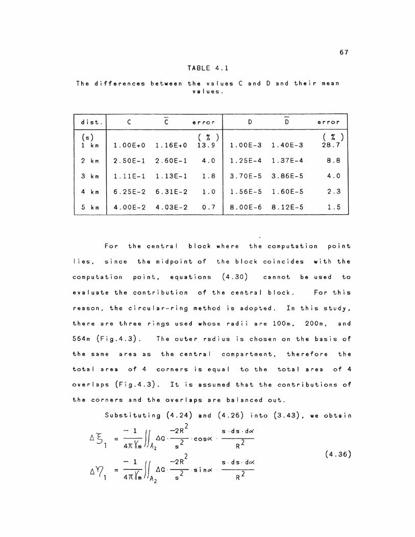
4.1. The differences between the values C and D and their mean values. 67

4.2.

4.3.

4.4.

4.5.

4.6.

5. 1.

5. 2.

5.3.

5.4.

5.5.

5.6.

5.7.

5.8.

5. 9.

Terrain profile contribution in flat area. 74

Terrain profile contribution in hilly area. 74

Terrain profile contributions referred to different distances r in a flat area. 77

Terrain profile contributions referred to different distances r in a hilly area. 77

Error budget for all of the values in (4.56).

The Stokes-Molodenskij curvature effect 1.

The Stokes-Molodenskij curvature effect 2.

The Stokes-Molodenskij curvature effect 3.

The Stokes-Molodenskij curvature effect 4.

The Stokes-Molodenskij curvature effect 5.

The Stokes-Molodenskij curvature effect 6.

at

at

at

at

at

at

station

station

station

station

station

station

83

86

87

88

89

90

91

The geoidal deflections predicted by program GDOVE. 93

The astro-gravimetric curvature effect (the difference between the geoidal deflection and the surface deflection). 97

Comparisons between the astra-gravimetric (A-G) and the Stokes-Molodenskij (S-M) curvature effects. 98

vi i

2. 1.

2.2.

2.3.

2. 4.

2. 5.

3 .1.

3.2.

3.3.

3.4.

3. 5.

3.6.

3.7.

3.8.

4 .I.

4.2.

4.3.

4.4.

4.5.

4.6.

LIST OF FIGURES

Equipotential surfaces and plumb I ines.

Geoid, quasigeoid and telluroid.

Gravity vectors on the actual and the.normal potential surfaces.

Surface deflection (or astra-geodetic deflection).

Molodenskij's deflection and geoidal deflection.

Geometry of a sphere and its sections:

Spherical approximation.

Consideration of the plumb I ine curvature effect for section AB.

A local astronomical coordinate system.

The north-south component of the plumb I ine cruvature effect.

Attraction of one compartment.

Normal and actual plumb I ine curvature effects.

Relationship between deflections and curvature effects.

Innermost and inner zones.

Innermost zone.

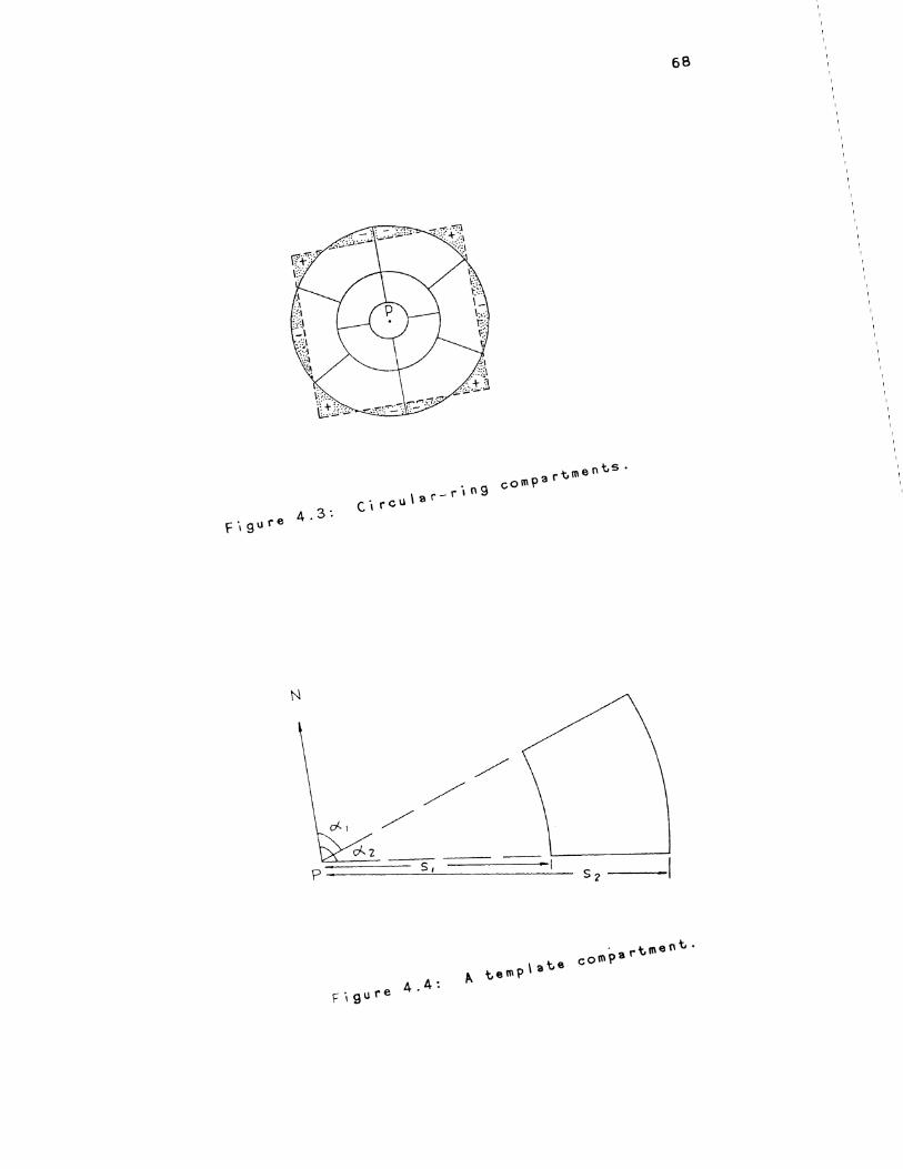
Circular-ring compartments.

A template compartment.

North-south terrain profile at computation point.

A trend for the terrain slope.

VI i i

9

13

15

21

22

25

29

35

37

41

42

44

47

54

55

68

68

75

78

4.7.

5. 1.

Zone boundary for the contribution of 6G.

Distribution of the tested stations in New Brunswick.

IX

. 80

. 85

The uti I ization

CHAPTER 1

INTRODUCTION

of the concepts of gravity and its

potential in geodesy can be classified into two groups: the

operation with the magnitude of gravity 1n the gravimetric

methods and the use of the direction of the gravity vector

in the astra-geodetic

point is tangential

methods. The gravity vector

to the plumb I in e at that

at any

point.

Because of the irregular density distribution of the earth,

the plumb I in e IS not a straight I in e but a curve.

Therefore, the astronomic observations made on the surface

of the earth are not identical to their corresponding values

on the geoid.

curvature of

The discrepancies arise from the effect the

the plumb I in e. In order to make these

quantities comparable, the correction of the curvature

effect of the plumb I ine must be taken into account.

For the determination of the geoid by means of the

astra-geodetic mehtod, the astra-geodetic deflections (or

surface deflections)

This reduction IS

must be reduced downward to the geoid.

achieved by taking into account the

curvature of the plumb I ine. The determination of the geoid

by the astra-gravimetric method also necessitates the

surface deflections and the goidal deflections to be

- 1 -

compatible.

application

plumb line.

This

of a

compatibility is brought through

correction due to the curvature of

2

the

the

A few researchers such as Helmert(1880), Graaff-

Hunter and Bomford(1928), Ledersteger (1955), Arnold(1956),

Ndyetabula(1974), Groten(1981) and others have investigated

the problem of the curvature of the plumb line. The plumb

I ine curvature effect of the actual gravity field IS more

important but ·extremely difficult to determine (Groten,

1981) . So far some approaches for the estimation of the

curvature effect of the plumb I in e have been developed:

using the gravitJ field models, using a relation between the

curvature effect and orthometric height correction, using

density models, and by using Meinesz's

Molodenskij's formulae together,

introduced in Chapter 3.

Vening

etc. These wi II

and

be

The curvature of the plumb line IS mainly due to the

topographic

the earth.

I in e up to

irregularity and the density distribution within

In the Alps, the curvature effects of the plumb

12" have been obtained (Kobold and Hunziker,

1962). Without knowledge of the density distribution inside

the earth,

obtained by

(Ndyetabula,

the accuracy of the plumb line curvature effect

using the first three methods is questionable

1974). Uti I izing the first two approaches, a

dense gravity net around the computation point is needed

Vening (Heiskanen and Moritz, 1967). With the use of

3

Meinesz's and Molodenskij's formulae, it becomes complicated

and time-consuming to compute the geoidal and Molodenskij's

deflections separately. Besides, the integrations should be

extended over the whole earth.

Using the above mentioned ways, the evaluation of the

curvature effect 1s a difficult task due to the fact that

sufficient gravity and height data or the data for the

density distribution inside the earth are necessary.

In this study, an alternative approach, developed by

Vant~ek and Krakiwsky (1982), is used to evaluate the effect

of the curvature of the plumb I ine. The method is based on

the combination of Stokes's

An analytical form is given

and Molodenskij's

of the difference

approaches.

between the

geoidal and Molodenskij's deflections. In this thesis, the

ana lyti ca I form is called the Stokes-Molodenskij formula.

This formula can compute the plumb line curvature effect

than Vening Meinesz's and Mo I ode n s k i j ' s more conveniently

formulae together. In addition, the distant zones can be

neglected without the loss of accuracy, and the density

distribution is not needed to determine the plumb I i n e

curvature effect.

If the geoidal and the surface deflections are known,

the pI umb ine curvature effect can be straightforwardly

determined. In this study, a comparison between the plumb

I ine curvature effect determined from the Stokes-Molodenskij

formula and that obtained from the geoidal and the surface

deflections IS made

Brunswick.

at s1x stations in the

4

province of New

A few definitions and basic philosophical backgrounds

are outlined in Chapter 2. In Chapter 3, Stokes's and

Molodenskij 's approaches for evaluating the deflections of

the vertical are g1ven briefly. Some approaches for

computing the plumb I ine curvature effect are also reviewed.

The mathematical development of the method combining

Stokes's and Molodenskij 's approaches to determine the

curvature effect is given.

For practical evaluation of the curvature effect of

the plumb line by means of the Stokes-Molodenskij formula,

there are two different zones needed: innermost and inner.

The data used include the point gravity anomalies and

heights, and the mean gravity anomalies and mean heights for

the 5x5 minutes blocks used. The estimation of the tangent

of the terrain inc( ination is rigorously treated to give a

reliable contribution to the plumb I ine curvature effect.

The possibi I ity of neglecting the distant regions beyond the

1nner zone without affecting accuracy is discussed in

Chapter 4.

There are s1x stations tested, two 1n mountainous

areas and four 1n flat areas. The results are presented in

Chapter 5. For convenience, the curvature effect determined

from the Stokes-Molodenskij formula 1s called the Stokes­

Molodenskij curvature effect, and the curvature effect

5

obtained from the geoidal and the surface deflections is

cal led the astra-gravimetric curvature effect.

between them is also shown in this chapter.

are given.

A comparison

The analysis

and explanation for the comparison Finally, a

few conclusions are drawn and recommendations are given for

further studies.

As a guide to the reader, the goal of each chapter IS

presented below:

1.

2.

The goal of Chapter 2 IS to review the

concepts for the gravity field of the earth

an insight into the topic. Three types

deflections of the vertical used in geodesy

differences among them were described.

general

and give

of the

and the

The goal of Chapter 3 is to review and relate the

different

effect of

approaches for evaluating the curvature

the pI u mb I in e. In addition, the

mathematical developement of the method based on

is combining Stokes's and Molodenskij 's approaches

also reviewed.

I in e curvature

The approach

effect without

can compute the plumb

the knowledge of the

density distribution inside

accuracy.

the earth and to a high

3. The goal of Chapter 4 is to perform a practical

evaluation of the Stokes-Molodenskij formula. It is

shown that the distant zones whose spherical

distan~es from the computation point exceed 13 can be

4.

6

loss of accuracy. In order to neglected without any

get reliable results, the evaluation of the terrain

slope was treated rigorously.

The goal of Chapter 5 is to demonstrate the

computational results and make comparisons between

the Stokes-Molodenskij and the astra-gravimetric

curvature effects. The comparisons show that the

model based on the Stokes-Molodenskij

give a much higher accuracy than

formula can

the astra-

gravimetric model. Besides, the former can be easily

applied to evaluate the curvature effect of the plumb

I in e.

A few contributions are made in this work.

summarized below:

These are

1.

2.

3.

First practical testing of the Stokes-Molodenskij

formula, developed by Vanf~ek and Krakiwsky (1982),

for the determination of the curvature effect of the

plumb I ine.

Development of an algorithm for numerical evaluation

of the Stokes-Molodenskij formula.

Formulation of an algorithm for terrain slope

evaluation.

CHAPTER 2

DEFINITIONS AND GENERAL BACKGROUND

A body rotating with the earth is subjected to the

gravitational force due to the mass of the earth and the

centrifugal force due to the earth's rotation. The sum of

the gravitational and the centrifugal forces is called the

force of gravity.

The magnitude of the force of gravity is not the same

everywhere on the surface of the earth; namely, it is a

function of position. The gravity force on the neighborhood

of the poles is greater than it is on the equator. In

addition, the gravity force undergoes temporal variations

resulting from the gravitational force of celestial bodies,

~rustal deformations, and tectonic deformations (Vanf~ek and

Krakiwsky, 1982).

There IS a potential corresponding to the gravity

force, called the potential of gravity, W. It is the sum of

the gravitational potential, denoted by Wg, and the

centrifugal potential, denoted by We (Heiskanen and Moritz,

1967):

W = Wg + We . (2.1)

- 7 -

8

The gradient vector of W,

g = \7111 (2.2)

is called the gravity field. The magnitude of g is measured

1n gals ( 1 gal

second squared.

adopted the more

= 1 cm.sec-2 = 1 dyne/g ) or in metres per

The sciences of geodesy and geophysics have

suitable unit--- the milligal ( 1 mga I =

The direction of the gravity vector is known as

the direction of the plumb line, or the vertical.

The term equipotential surface means a surface on

which the potential W is constant. The general equation of

an equipotential surface is expressed by

W( r ) = const. (2.3)

It is a continuous and smooth surface. Although an infinite

number of equipotential surfaces can be accredited by

different values to the potential, they never intersect one

another. The equipotential surfaces define the horizontal

direction; thus they are also called level surfaces. The

lines of gravity force norma I to the earth's equipotential

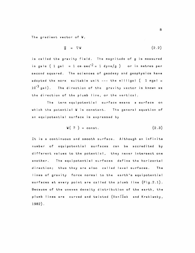
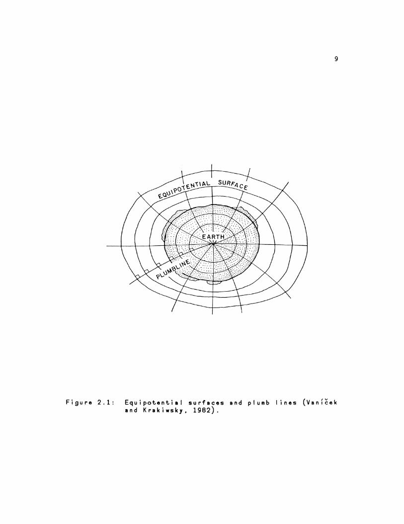
surfaces at every point are called the plumb line (Fig.2.1).

Because of the uneven density distribution of the earth, the

plumb lines are curved and twisted (Vanf~ek and Krakiwsky,

1982).

9

Figure 2.1: Equipotential surfaces and plu~b lines (Vanfcek and Krakiwsky, 1982).

10

The Bureau Gravimetrique Internationale in Paris, an

institution of the IAG, maitains worldwide gravity data. A

few mi I I ion observations show that the magnitudes of gravity

vary locally and regionally. Due to the elevation of

stations, the oblateness of the earth, and the uneven mass

distribution within the earth, the variations reach more

than 5 gals for the magnitude of gravity g (Vanf~ek and

Krakiwsky, 1982).

For geodetic purposes, a reference gravity field is

selected such that the average difference between this field

and the actual gravity field is as smal I as possible. An

approximate represention of the actual gravity potential may

be achieved by an ellipsoid.

A reference e I I ipso i d is an e I I ipso i d of revolution

which 1s an equipotential surface of a normal gravity field.

It is also ca I I ed the I eve I e I I ipso i d. The reference

el ipsoid possesses t.he following charact.eristics:

1.

2.

3.

The mass of

t.otal mass of

at.mosphere.

t.he reference ellipsoid is

t.he eart.h, including t.he

equa I t.o the

mass of t.he

It spins around its minor axis wit.h the same angular

velocity as t.hat. of the eart.h.

Its cent.er coincides

earth.

with the gravity center of the

11

The reference ellipsoid generates a reference gravity

field, called normal gravity field. A reference potentia I,

denoted by U, is usually adopted to approximate the actual

potential.

is given by

In analogy to (2.2), the normal gravity vector

"f = \lU. (2. 4)

The Geodetic Reference System 1967(GRS67), a geocentric

equipotential ellipsoid, adopted at the XIV General Assembly

of IUGG in 1967, represents

field of the earth. The

the size, shape,

primary geometric

and gravity

ellipsoidal

parameters are:

equatorial radius( major semJ-ax1s ) a = 6378160 metres

flattening of reference ellipsoid f = 1/298.247.

The corresponding normal gravity

given by

r of level ellipsoid is

Y = 978031.8(1+0.005 3024·sin2~-0.000 0059·sin2 2¢) mgals.

(2.5)

It was perceived that GRS67 no longer approximates the

actual figure and gravity field of the earth to an adequate

accuracy. Therefore, it was replaced by the Geodetic

Reference System 1980,

geocentric equipotential

also based

e I I ipso i d

parameters are a= 6378137 metres

on the theory of

(Moritz, 1980a).

and f=1/298.257.

international gravity formula(1980) is given by

the

The

The

12

r = 978032.7(1+0.005 3024·sin2¢-0.000 0058·sin2 2¢) mgals,

(2.6)

where 1s the latitude of station.

The geoid IS an equipotential surface of the earth's

gravity field which IS approKimately represented by mean sea

level. The geoid IS known as the datum for orthometric

height system. Besides, the geoid is often referred to as

the figure of the earth, because it closely approKimates

about 72% of the terrestrial globe.

The separation between the geoid and a reference

ellipsoid is the geoidal height N (Fig.2.2). At present,

there are several possible methods of geoid determination:

gravimetric method, astro-geodetic method, astro-gravimetric

method, sate I I ite geodynamics, satellite altimetry, direct

determination from 3D positions and orthometric heights

(Rizos, 1982). etc. It is not within the scope of this

thesis to give a description of alI the techniques.

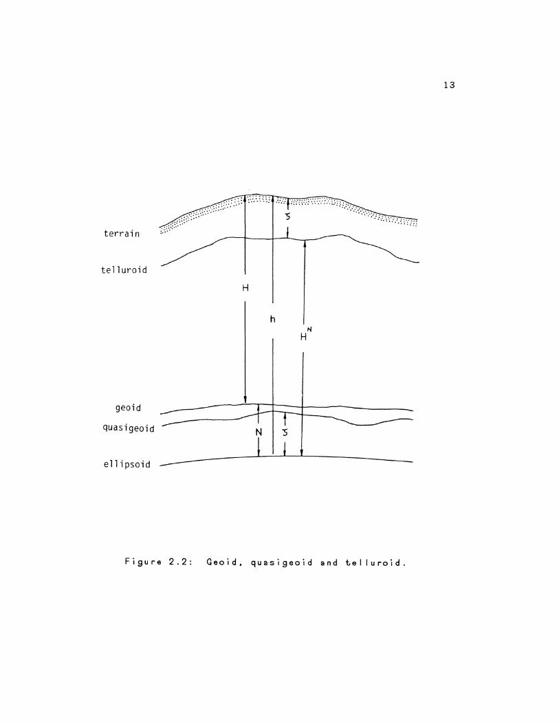
terrain

telluroid

geoid

quasi geoid

ellipsoid

H

h N

H

Figure 2.2: Geoid, quasigeoid and telluroid.

13

14

For the gravity field of the earth, the actual

potential W at any point can be expressed by the sum of a

normal potential U and a small remainder T:

w( -r )= u( -r) + r( -r ) . (2.7)

or

T( -r )= w( -r ) - u( r ) (2.8)

The difference T between the actual potential and the normal

potential 1s called disturbing potential, or anomalous

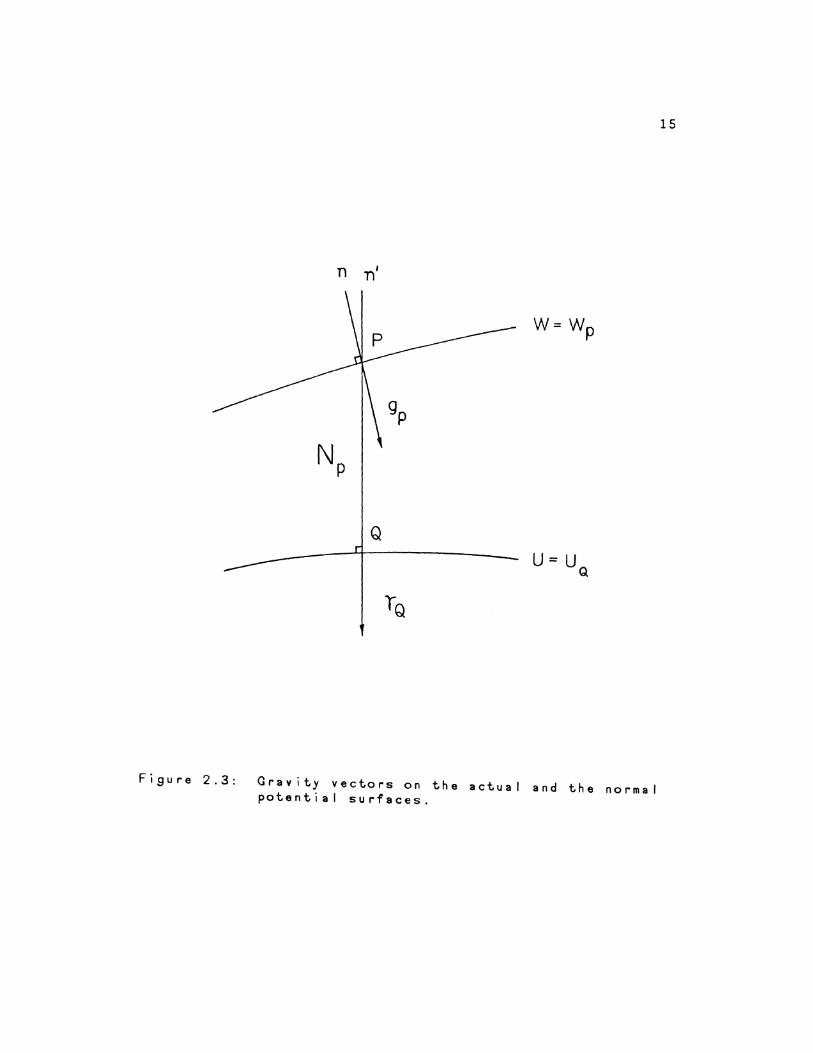
potential. Similarly, the gravity gat P is approximated by p

the corresponding normal gravity YQ at point Q on the

equipotential surface U=UQ(Fig.2.3).

The difference in magnitude between them is known as

the gravity anomaly at the point P:

.1g = I 9 I - If I . p Q

(2.9)

The vertical gradient ofT is given by:

\] T ( r ) = \7 (W ( r ) - U ( r ) ) = \7 (W - U ) • p p p p p

(2. 10)

After inserting (2.2) and (2.4) into (2.10), the vertical

gradient of the disturbing potential becomes

\/ T = = g - ¥ p p

(2.11) On,

were n' is the ellopsoidal normal (FiQ.2.3).

n n'

Q

U=U Q

Figure 2.3: Gravity vectors on the actual and the normal potential surfaces.

15

16

The normal gravity ~p at point P may be evaluated by the

following linear form (Heiskanen and Moritz, 1967, p.85):

tp 3" 0 <t

= + --· N ~ a n, p

(2.12)

Substituting (2.12) into (2.11) yields

OT d ~ = g t N

an, p Q d n' p (2.13)

or

OT a~ = ll g - N

On' 0 n' p (2.14)

Since the relation between the geoidal height and the

disturbing potential is given by Bruns as (Ibid., p.BS)

T N = (2.15)

and if the directions of geoidal normal n and ellipsoidal

normal n' are considered to almost coincide, equation (2.14)

becomes

T = fl g . __Q_

~p (2.16)

Rearranging (2.16) and disregarding the subscripts, we have

1 0 . (2.17)

17

This expression 1s known as the fundamental equation of

phys i ca I geodesy.

Two reference surfaces, the reference e IIi psoid and

the geoid, are used in the conventional approach to the

determination of the figure of the earth. Molodenskij

proposed a different approach in 1945. In Molodenskij's

approach the reference surface is no longer the geoid but

t.he telluroid. There are two different surfaces defined in

this approach, telluroid and quasigeoid. The quasigeoid

does not have a physical interpretation, except at sea.

The telluroid 1s originally defined as the locus of

points whose normal potential U is equal to the actual

potential Wp at the surface of the earth. On the other

hand, the telluroid can also be defined as a locus of normal

N heights H measured along the normal plumb line from the

reference ellipsoid (Vanf~ek, 1974).

The separation between the terrain and the tel luroid

is called height anomaly, denoted by"$. A I oc us of height

a noma I i es reckoned along the normal plumb line from the

ellipsoid is known as the quasigeoid.

From fig.2.3 the relationship between the height

anomaly S and the geoidal height N can be deduced from the

following equations:

N = h - H ,

(2.18)

(2.19)

18

where his ellipsoidal height, and H is orthometric height.

It is instructive to compare the height anomaly and geoidal

height. Combining equations (2.18) and (2.19) yields

N N-5=H -H. (2.20)

This difference 1s fairly sma I I and elevation-dependent.

For instance, the difference is about -1.8 m for Mt. Blanc

in the Alps (Arnold, 1960). In the open ocean the geoid and

quasigeoid coincide, so N=3

The deflection of the vertical is defined as the

spatial angle between

actual ~ravity vector.

the normal gravity vector and the

The deflection of the vertical can

be decomposed into two orthogonal components, the north-

south (along the astronomical meridian) and the east-west

(in the prime vertical) components, denoted by '§ and Y( .

For instance, if the geodetic reference ellipsoid is aligned

to the Conventional Terrestial coordinate system(CT), and if

astronomic coordinates and geodetic coordinates are denoted

by (p.A) and (¢ . .A). respectively, then the components of

the deflection of the vertical are given by:

5 = ~ - <P

Y( = (A- .A) ·cos¢ (2.21)

19

The origin of the CT system 1s at the centre of mass of the

earth, z-axis points to the Conventional International

Origin(CIO), the xz-plane contains the mean Greenwich

Observatory, and they-axis 1s selected to make the system

right-handed.

The deflection obtained can be either absolute or

relative according to which kind of reference e I I i pso i d 1 s

adopted. If a non-geocentric ellipsoid is used, it w iII

result in the relative deflection of the vertical The

deflection, however, 1s absolute when the adopted reference

ellipsoid is geocentric.

It should be mentioned here that there are three

species of deflection used 1n geodesy. These are:

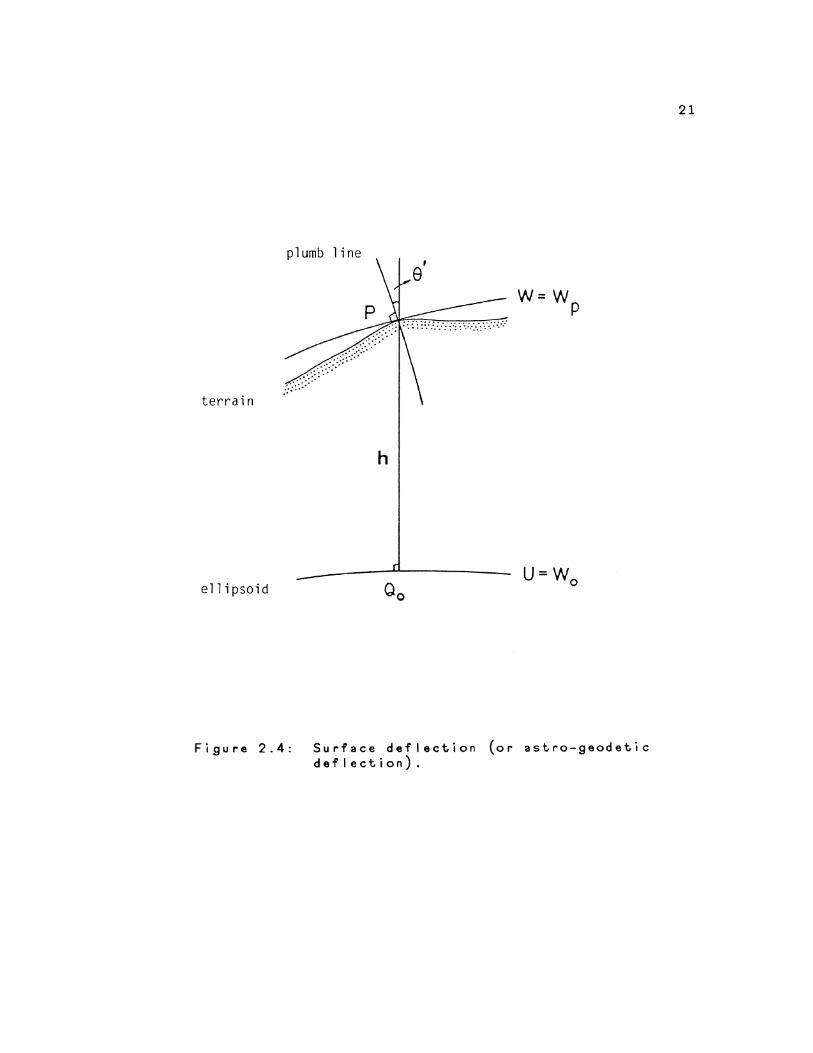
1. The surface deflection of the vertical a', defined as

the angle at the surface of the earth between the

directions of the plumb I ine and the normal (through

point P) to the reference ellipsoid (Fig.2.4). The I I

deflection components are denoted by S and 'fl . The

surface deflection can be obtained from astronomic

observations. The actual or normal gravity is not

required.

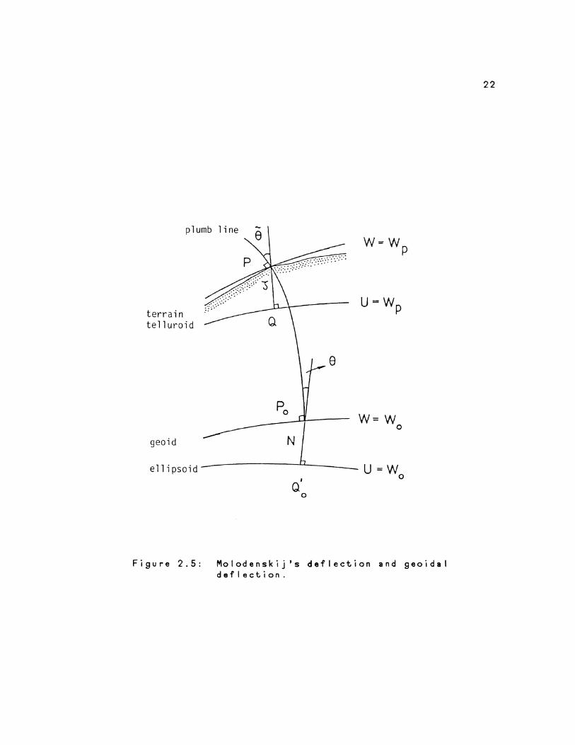
2. The geoidal deflection of the vertical 9 1s defined

as the angle (on the geoid) between the directions of

the plumb line and the e I I ipso ida I norma I (through

point Po), see Fig.2.5. The components of the

deflection are denoted by S and 'Q

20

"" 3. Molodenskij's deflection of the vertical 8 IS defined

by Molodenskij as the angle between the directions of

the plumb line (at point P) and the normal (through

point P) to the telluroid (Fig.2.5). The deflection -components are denoted by 5 and '?.

Clearly, due to the curved and twisted plumb line the

surface and geoidal deflections for the same point (with

respect to the same reference e I I ipso i d) are different.

Ordinarily, the differences between them are expected to be

more significant in mountainous areas than in the flat-

terrain regions. In the Alps. the differences of up to 12"

have been obtained by Kobold and Hunziker(l962).

The surface deflections are also different from

Molodenskij 's deflections. The deviation coming from the

curvature of the normal plumb line between the ellipsoid and

the te I I u ro i d is a function of the latitude and height of

the computation station. Greater differences occur at the

higher elevations.

plumb line

terrain

ellipsoid

Figure 2.4:

h

Surface deflection deflection).

W=W p

U=W 0

(or astro-geodetic

21

plumb line

terrain telluroid

geoid

W=W p

U=W p

W=W 0

e 11 i psoi d --------L..L. ____ U = W 0

I

Q 0

Figure 2.5: Molodenskij 's deflection and geoidal deflection.

22

CHAPTER 3

MATHEMATICAL DEVELOPMENT FOR THE CURVATURE EFFECT OF THE PLUMB LINE

The geoidal deflection mentioned 1n the

chapter is the angle between the actual gravity

preceding

vector on

the geoid and the normal gravity vector on the reference

e I I ipso i d. The determination of the geoidal deflections is

one of the tasks in geodesy, since it is usually required

for geodetic purposes. In Stokes's approach to the geodetic

bound a r y- v a I u e problem the geoid serves as a physical

reference surface. It must be assumed that there are no

masses outside the geoid, otherwise the theorem of Stokes is

not valid to determine the deflection of the vertical as

wei I as the geoid by means of gravity. In fact, there are

masses above the geoid, so they must be either completely

removed or moved inside the geoid. For this reason, some

assumptions and hypotheses concerning the density of mass

above the geoid must be made. The gravity measured on the

surface of the earth, therefore, has to be reduced downward

to the geoid.

If gravity has already been reduced to the geoid

appropriately, then the· gravity anomaly ~g on the geoid can

- 23 -

24

be obtained. In geodesy, the free-air gravity anomalies are

used to determine the geoidal height and the geoidal

deflection of the vertical. The derivation of the formulae

for determining the deflections has been described in a few

texts( e.g. Heiskanen and Vening Meinesz, 1958; Heiskanen

and Moritz, 1967; Vanicek and Krakiwsky, 1982). It wi II not

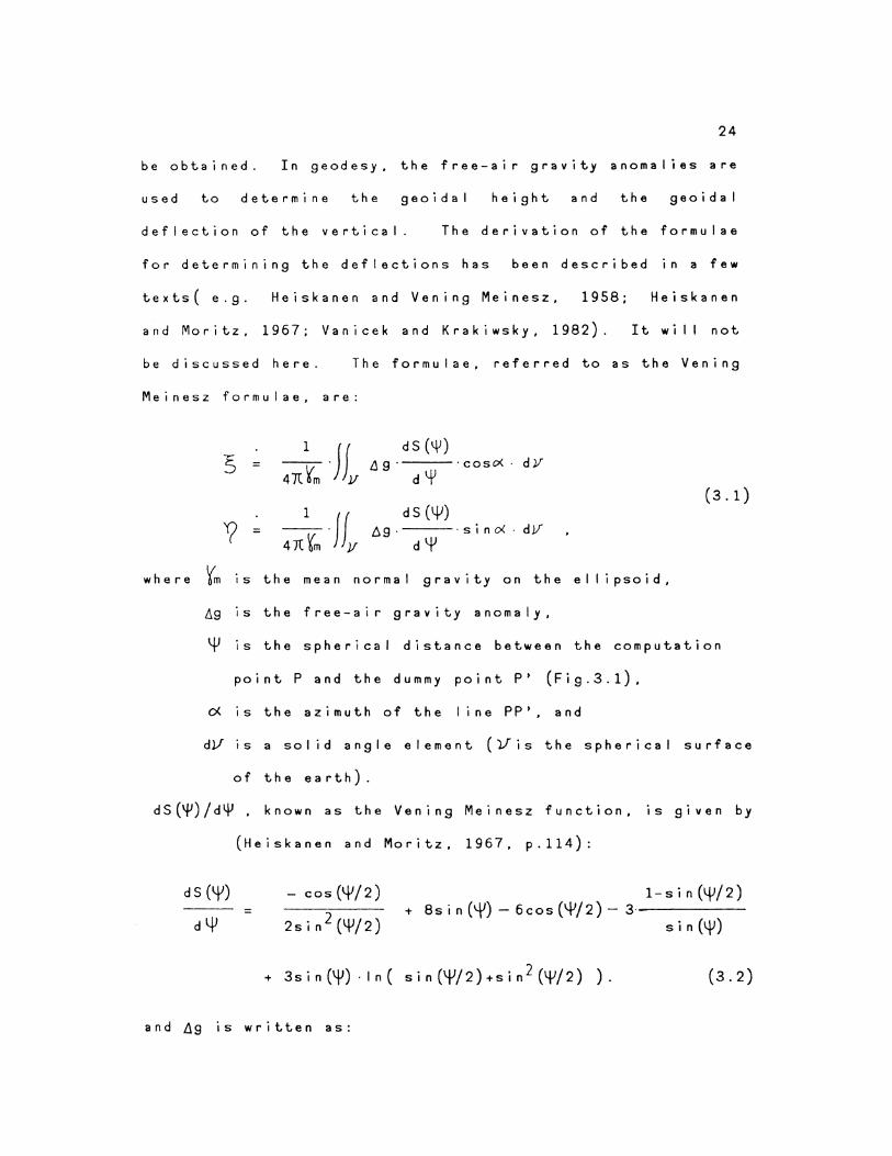
be discussed here. The formulae, referred to as the Vening

Meinesz formulae, are:

= 41C~m -Jflf dS (~)

ll9" ·coso<· dV d~

4 711~. J JJI

d s (41) ll9 . ·sino< · dV

dYJ =

w h e r e Ym 1 s t h e m e a n n o r m a I g r a v i t y o n t h e e I I i p s o i d •

~g 1s the free-air gravity anomaly,

( 3. 1)

l.tJ IS the spherical distance between the computation

point P and the dummy point P' (Fi9.3.1),

o< IS the azimuth of the line PP', and

dl.f 1 s a so I i d an 9 I e e I em en t ( 1f i s the s ph e r i c a I s u r face

of the earth).

dS(~)/d~ . known as the Vening Meinesz function, IS given by

(Heiskanen and Moritz, 1967, p.114):

d s (YJ)

d4J =

- cos ('+'I 2 )

2sin 2 (tVI2)

1-sin(I.{JI2) + 8s in(~)- 6cos ('+'12)- 3----­

s i n (\.jJ)

+ 3 s i n (\fl) · I n ( s i n (\f) I 2) + s i n 2 (~I 2) ) . (3.2)

and .19 1s written as:

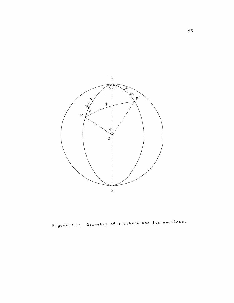
Figure 3.1:

N

'-.... I I '-.... I I

'-....~ o:

I I

s

Rf-

I I

I

Geometry of a sphere and its sections.

25

26

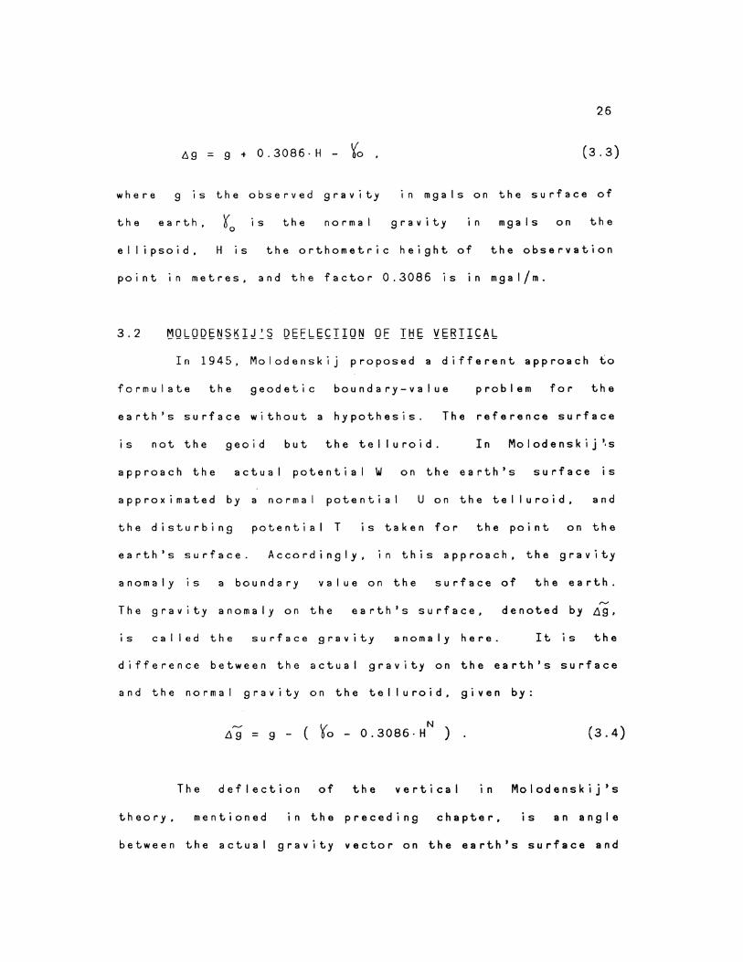
6. g = g + 0 . 3 0 8 6 · H - Yo , (3. 3)

where g IS the observed gravity 1n mgals on the surface of

the earth, v is 00 the normal gravity in mgals on the

e I I ipso i d, H is the orthometric height of the observation

point in metres, and the factor 0.3086 is in mgal/m.

In 1945, Molodenskij proposed a different approach to

formulate the geodetic boundary-value problem for the

earth's surface without a hypothesis. The reference surface

IS not the geoid but the telluroid. In Molodenskij~s

approach the actual potential W on the earth's surface is

approximated by a normal potential U on the telluroid, and

the disturbing potential T is taken for the point on the

earth's surface. Accordingly, in this approach, the gravity

anomaly is a boundary value on the surface of the earth.

The gravity anomaly on the earth's surface, denoted by flg,

is called the surface gravity anomaly here. It is the

difference between the actual gravity on the earth's surface

and the normal gravity on the telluroid, given by:

= g - ( Yo- 0.3086-HN ) (3.4)

The deflection of the vertical 1n Molodenskij 's

theory. mentioned in the preceding chapter, is an angle

between the actual gravity vector on the earth's surface and

27

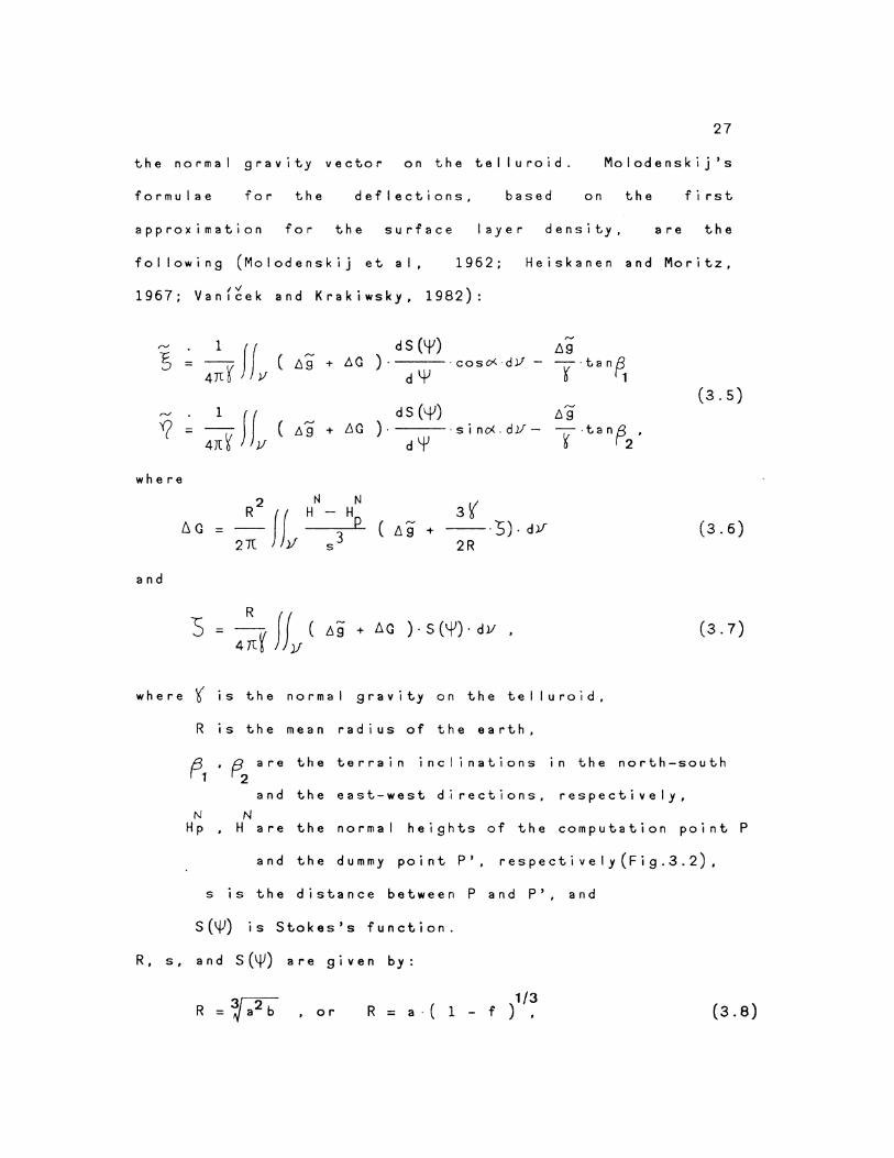
the normal gravity vector on the telluroid. Me I aden ski j 's

formulae for the deflections, based on the first

approximation for the surface layer density, are the

following (Molodenskij et al, 1962; Heiskanen and Moritz,

/V ) 1967; Vanacek and Krakiwsky, 1982 :

,..._

4:~ ffv ( d s (lf') ,6g

5 "" = .69 + 6G )· · cosol.·dJ/- y·tan~ dYJ

(3. 5) "' 4~~ J fv (

d s (l.jl) 6g Y( ....-

+ fiG ) . · s i no<. dl.f- T·tanp2 • = 6g d't'

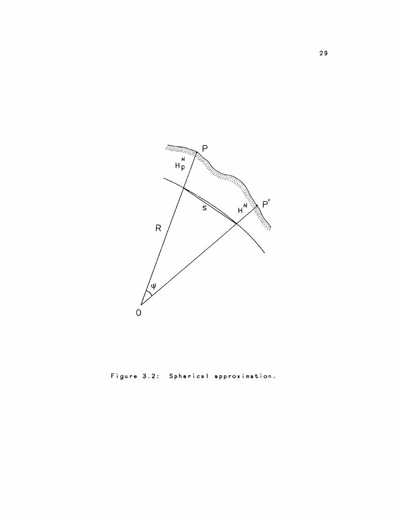
where

2 N N 3~

_R ff H - Hp /).Q = ( llg + --·:S). d.ll 21l }/ s 3 2R

(3.6)

and

5 = 4:r It ( .69 + ll G ) · S (~) · d lf , (3.7)

where'{ is the normal gravity on the telluroid,

R is the mean radius of the earth,

{31 •(3. are the terrain inclinations in the north-south 2

and the east-west d~rections, respectively, N N

Hp ' H are the normal heights of the computation point p

and the dummy point P', respectively(Fig.3.2),

sis the distance between P and P', and

S(~) is Stokes's function.

R, s, and S(~) are given by:

R = ~ a2 b , or 1/3

R =a·( 1- f) , (3.8)

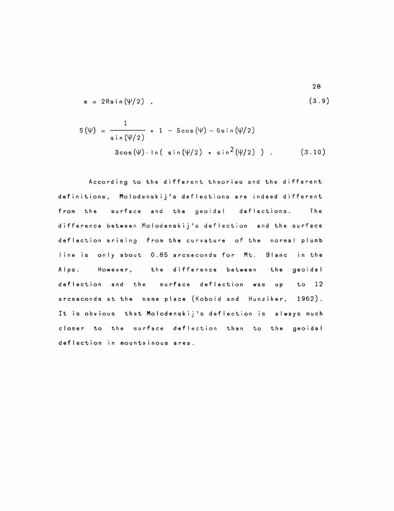
s = 2Rsin(~/2)

S(lfl) = 1

+ 1 - Scos (YJ) - 6s in (~/2) sin(I.Jl/2)

3cos(4')·1n( sin(\f'/2) + sin2(lp/2))

28

(3.9)

(3.10)

According to the different theories and the different

definitions, Molodenskij's deflections are indeed different

from the surface and the geoidal deflections. The

difference between Molodenskij 's deflection and the surface

deflection arising from the curvature of the

line is only about 0.85 arcseconds for Mt.

Alps. However, the difference between

normal plumb

81 an c in the

the geoidal

deflection and the surface

arcseconds at the same place

deflection

(Kobold and

was up

Hunziker,

to 12

1962).

It is obvious that Molodenskij's deflection is always much

closer to the surface deflection than to the geoidal

deflection in mountainous area.

29

R

0

Figure 3.2: Spherical approxima~ion.

30

3.3 ~Q~~ I~~~~IQV~~ EQB ~Q~EVII~Q I~~ ~V8~~IV8~ ~EE~~I QE I~~ E!:V~~ !:;!;ti~

The plumb line, the so-called line of gravity force,

IS bent and twisted. Some of the geodetic measurements on

the physical surface of the earth, e.g. triangulation and

level ling, make use of the plumb in e. For some geodetic

missions, the influence of the curvature of the plumb I ine

should be taken into account when the reduction of geodetic

or astronomic observations to the geoid or to the ellipsoid

1s needed. No matter how the plumb lines bend and twist

within the earth, the curvature effect of the plumb I ine

between the earth's surface and the geoid is usually

considered 1n the field of geodesy. That is to say, that

the deviation between the gravity vector on the earth's

surface and the gravity vector on the geoid IS investigated.

It is also convenient for geodetic purposes to decompose the

curvature effect, denoted by li 8 • into the north-south

component .15 and the east-west component t:,Y( as the same way

as the deflection of the vertical is decomposed.

There are a few ways of determining the curvature

effect of the plumb I ine: by using the gravity field models,

by using a relation between the curvature effect and

orthometric height correction, by using density models, by

using Vening Meinesz's and Molodenskij's formulae together,

etc.

31

3.3.1

Taking the origin at the computational point, we set

up a rectangular coordinate system xyz with z-axis along the

vertical and the x- and y-axes on the horizontal plane

pointing northwards and eastwards, respectively. Such a

system is called the Astronomical system(LA).

The two orthogonal components of the plumb I in e

curvature effect are given by (Heiskanen and Moritz, 1967):

()g -·dh dx

ag -·dh ih ·

(3.11~

where H 1s the orthometric height of the computation point.

In order to evaluate the above integrals, a knowledge of the

gravity and its horizontal gradients at every point along

the plumb I i ne is necessary. Because the density

distribution and the gravity variations inside the earth are

not well-known, it is difficult to evaluate the curvature

effect of the plumb line from these formulae.

If the actual gravity g IS replaced by the normal

gravity r in the equation (3.11). the curvature effect of

the normal plumb I ine wi I I be obtained. Using (2.5), we

obtain the curvature effect of the normal plumb I ine:

32

N " LIS=- 0.17·sin2¢·H (3.12)

N fj,Y? = 0 •

where His the orthometric height in kilometres. Since the

normal gravity field is independent of longitude, the east-

west component is zero.

3.3.2 V~lng ~b~ r~l~~l2n ~~~~~~n ~~rY~~~r~ ~ff~~~ !n2 2r~b2m~~rl~ ~2rr~£~l2n

This approach is developed on the basis of a relation

between the actua I pI umb I i ne curvature effect (From now on

we ~hall leave out the word "actual".) and the orthometric

height correction. The curvature effect of the plumb line

is given by the following formulae (Heiskanen and Moritz,

1967):

+

(3. 13)

= +

where g IS the mean gravity along the plumb I ine. In order

to get reliable results, a dense gravity net around the

computation point is necessary to determine the horizontal

gradients of mean gravity o9/dx and o9! oy. and the

determination of mean gravity g along the plumb line must

be accomplished carefully. Even though horizontal gradients

33

of gravity are less sensitive to smal I density variations

than vertical gravity gradient, they are difficult to

evaluate precisely (Groten, 1981).

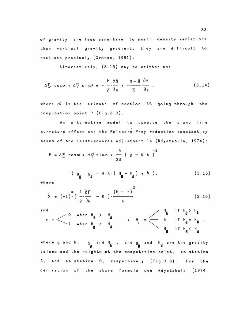
Alternatively, (3.13) may be written as:

.6 S ·cos d- + IJ. Y? · s i no<. = H OS

g Os +

g- s aH

g Os (3.14)

where of.. 1s the azimuth of section AB going through the

computation point P (Fig.3.3).

An alternative model to compute the plumb line

curvature effect and the Poincar~-Prey reduction constant by

means of the least-squares adjustment Is (Ndyetabula, 1974):

h -1 F = ..6'5-coso< + li"?·sino<- + -·( g- K·h)

2S

·(g-g -4·K·(H-H)+&), 8 A 8 A

where

m 1 ay 5 = (-1)·(

2 oh

2 (H. - h)

- K ) • ----~. __

h

and

/ <: when HB > HA m = H. = --

when H < H I

"" 8 A

where g and h • 9 and H and g8 and HB A A

HA

h

H8

are

values and the heights at the computation point,

(3.15)

(3.16)

if HB > HA

if H = 8 HA

if H 8< HA

the gravity

at station

A, and at station 8, respectively (Fig.3.3). For the

derivation of the above formula see Ndyetabula (1974,

34

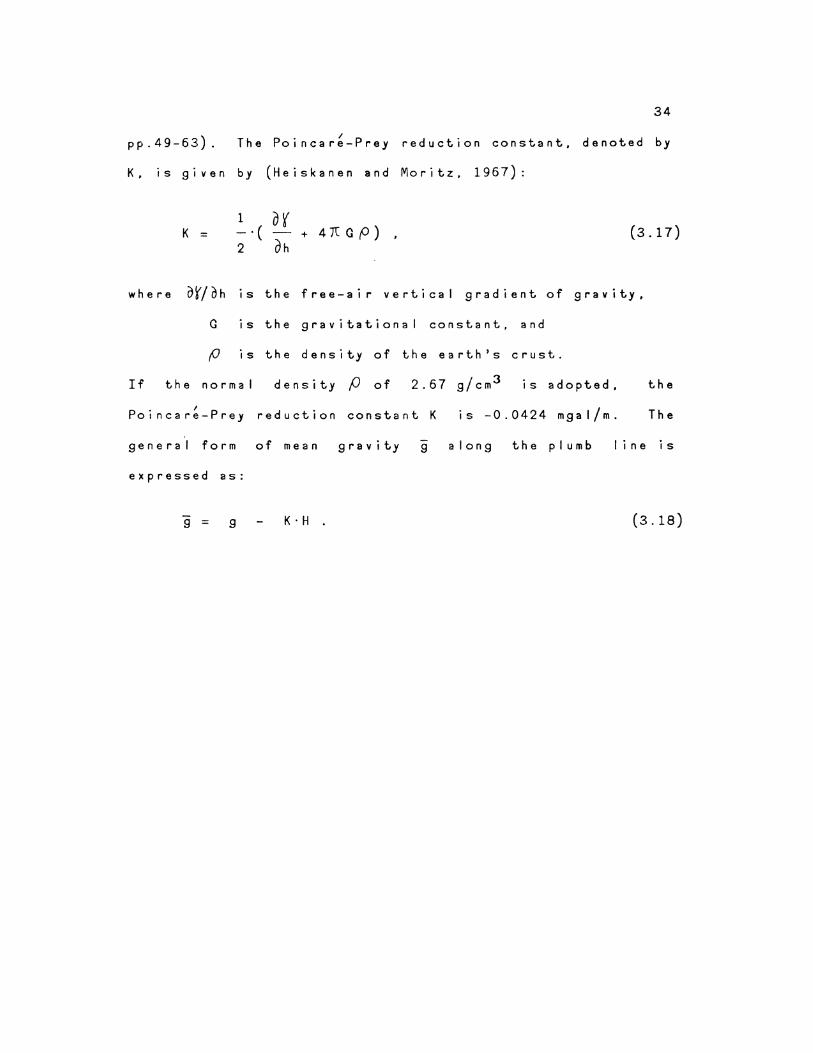
pp.49-63). The Poincar~-Prey reduction constant, denoted by

K, is given by (Heiskanen and Moritz, 1967):

K = 1 or -·(-+47LO,.O) 2 oh

(3.17)

where o~/Clh is the free-air vertical gradient of gravity,

Q is the gravitational constant, and

p is the density of the earth's crust.

If the normal density fJ of 2.67 g/cm 3 is adopted, the

Poincar~-Prey reduction constant K is -0.0424 mgal/m. The

general form of mean gravity g along the plumb I in e is

expressed as:

g = 9 K · H • (3.18)

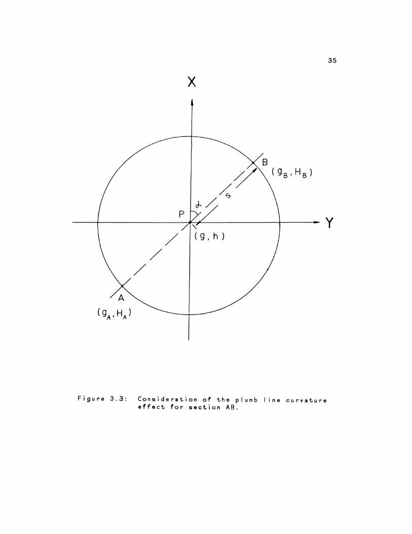
35

X

" y

/ /

/

( g ' h )

Figure 3.3: Consideration of the plumb I ine curvature effect for section AB.

36

3.3.3

The point P on the earth's surface and the

corresponding point Po on the geoid are subjected to

different gravity forces. The direction of the vertical

changes from the earth's surface to the geoid due to the

irregular mass distribution inside the earth's crust. If

the dens.ity distribution IS known, the deviation between

these two directions of the vertical can be determined by

Newton's law of gravitation.

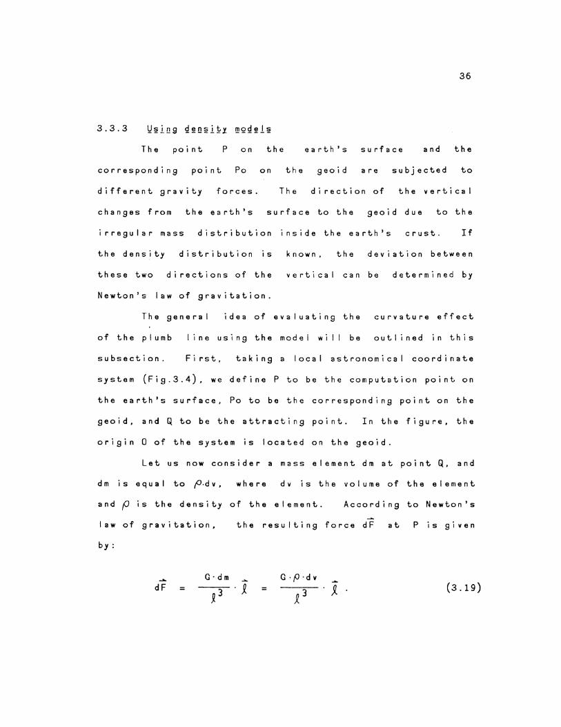
The general idea of evaluating the curvature effect

of the plumb line using the model will be outlined in this

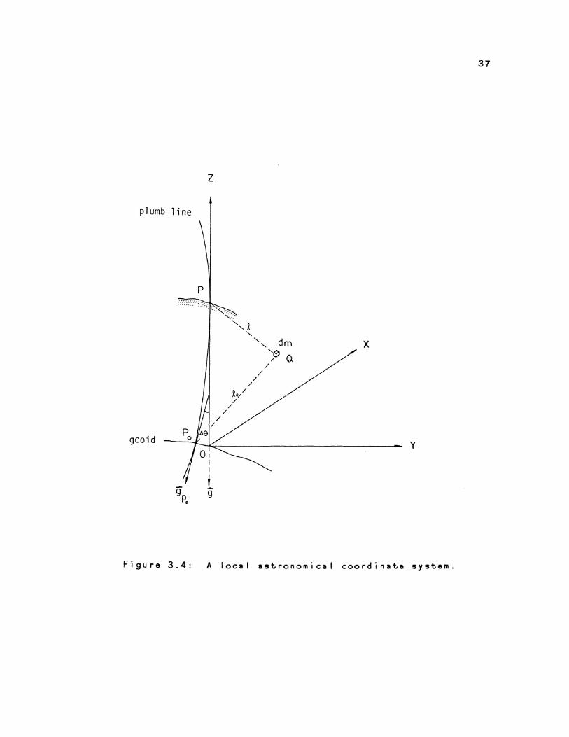
subsection. First, taking a local astronomical coordinate

system (Fig.3.4), we define P to be the computation point on

the earth's surface, Po to be the corresponding point on the

geoid, and Q to be the attracting point. In the figure, the

origin 0 of the system is located on the geoid.

Let us now consider a mass element dm at point Q, and

d m 1 s e qua I to p.d v , where dv is the volume of the element

and pis the density of the element. According to Newton's

law of gravitation,

by:

..... G·dm dF =

~3

..... the resulting force dF at

= G ·P ·dv

}.3

Pis given

(3.19)

37

z

plumb line

X

geoid y

Figure 3.4: A local astronomical coordinate system.

38

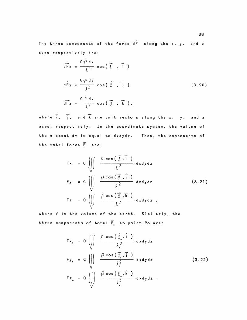
The three components of the force dF along the x, y, and z

axes respectively are:

G·P·dv dFx = ~2

cos ( ~ )

GP·dv cos c r dFy = ~2

j ) (3.20)

G·P·d v dFz = J-2

cos( J_ k ) •

where I' j . and k are unit vectors along the X' y • and z

axes, respectively. In the coordinate system, the volume of

the element dv IS equal to dxdydz. Then, the components of

the total force F are:

Jff P·COS (I .i )

Fx = G R2

·dxdydz

v

JfJ P·COS (I . j )

(3.21) Fy = G ~2

·dxdydz

v

JJJ p.cos cr ,k )

Fz = G ~2

·dxdydz . v

where v IS the volume of the earth. Simi I arty, the

three components of total F at point Po are: •

JJ f p.cosC[.i )

F x. G .

·dxdydz = J_2

v .

JJJ p.cos ( T •· j )

(3.22) F y • G • ·dxdydz = J2 v . jjf P·COS < r • k )

Fz G .

·dxdydz = ~2

v .

39

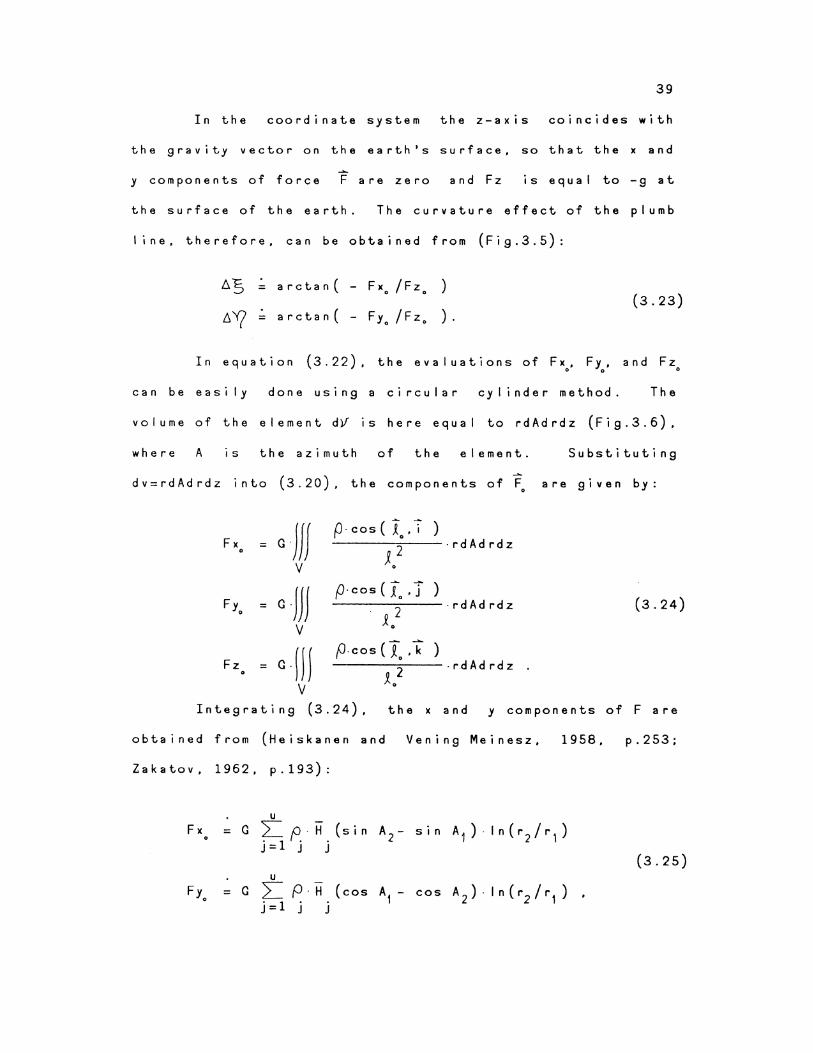
In the coordinate system the z-axis coincides with

the gravity vector on the earth's surface, so that the x and ~

y components of force F are zero and Fz is equal to-g at

the surface of the earth. The curvature effect of the plumb

line, therefore, can be obtained from (Fig.3.5):

arctan( - Fx./Fz. )

arctan( Fy. /Fz. ) . (3.23)

In equation (3.22), the evaluations of Fx, Fy, and Fz • • •

can be easily done using a circular cylinder method. The

volume of the element dV is here equal to rdAdrdz (Fig.3.6),

where A 1s the azimuth of the element. Substituting

dv=rdAdrdz into (3.20), the components of~ are given by:

Fx • G .Jff P·cos(T •. T )

= J.. 2

·rdAdrdz

v •

G -JJJ p·cos(t.j )

= J. 2

·rdAdrdz (3.24)

v •

Fy •

G. fJ J fJ·COS cr. ,k )

= J. 2 ·rdAdrdz

v . Fz

Integrating (3.24), the x and y components of Fare

obtained from (Heiskanen and Vening Meinesz, 1958, p.253;

Zakatov, 1962, p.193):

u Fx = G L p · H (sin A2- sin A1 )-1n(r 2 /r 1 )

j=1 j j (3.25)

u Fy = G ~ P·H (cos A1 - cos A2)-ln(r2 /r1 ) ,

• j = 1 j j

40

where A1 and A2 , r 1 and r2 are the boundaries of the compartment,

u is the number of the compartments,

p. is the density of the j-th compartment, and J

H. is the mean height above the geoid of the compartment. J

The component Fzo can be approximated by -g at the computation

point P:

(3.26)

Unless the density distribution around the point of

computation is wei known, to calculate the curvature effect

of the plumb line, as!Sumptions concerning the density must

be made and the heights around the computation point are

required. If the assumption that the density is constant is

made, on I y the terrain effect on the plumb line is taken

into account without considering the effect of the density

distribution. In this approach the uncertainties in

estimating the density distribution inside the earth are the

predominant error sources. If the distribution of density

is not we I I known, the errors may be very large (Zakatov,

1962).

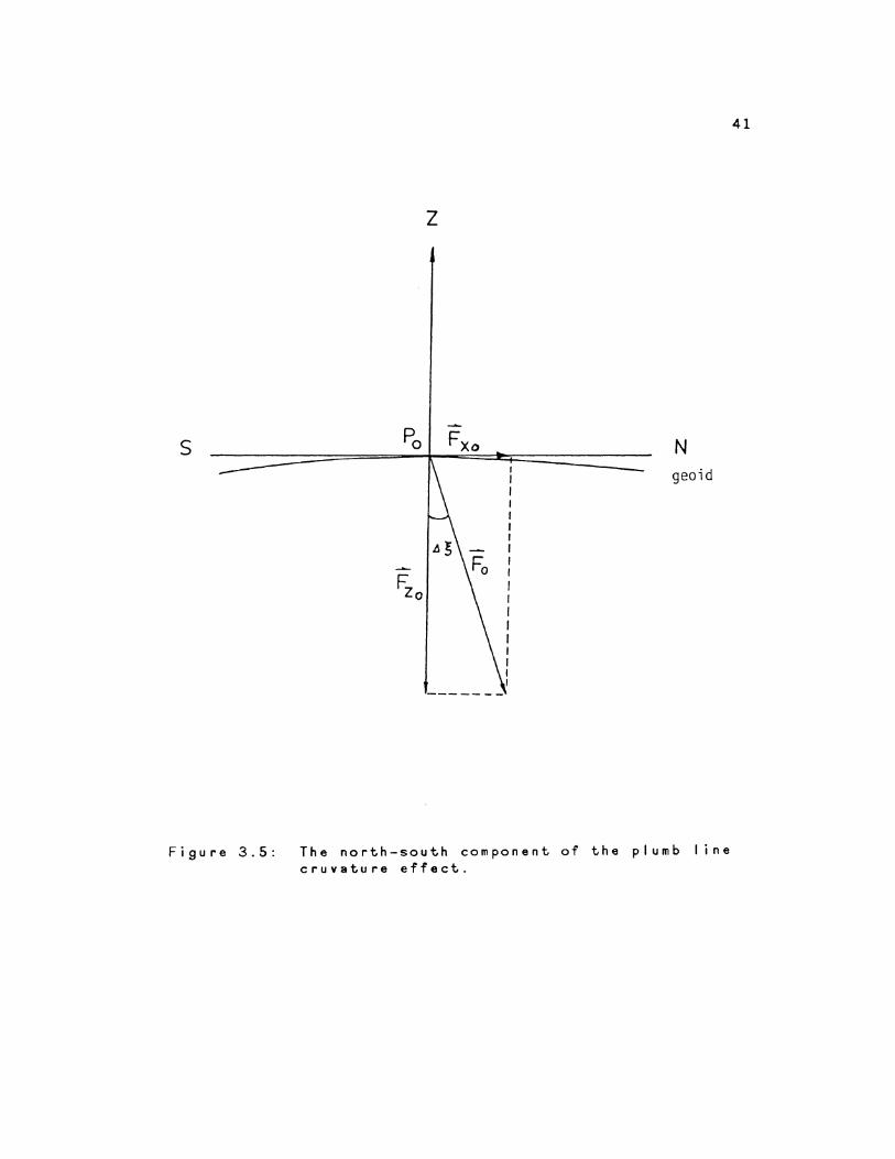
s

Figure 3.5:

z

N geoid

The north-south component of the plumb I ine cruvature effect.

41

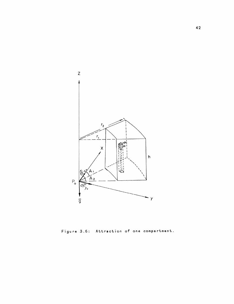
42

z

h

g y

Figure 3.6: Attraction of one compartment.

43

3.4 ~IQ~E~=~QLQQE~~~IJ ~EitlQQ EQB ~g~e~II~Q ItlE ~~B~~I~BE EEEE~I

The methods of determing the curvature effect of the

plumb line outlined in the preceding sections can be

regarded as direct ways to compute the deviation between the

actual gravity vector on the earth's surface and the actual

gravity vector on the geoid. In this section, the possible

way of utilizing the geoidal deflection and Molodenskij's

deflection to estimate the plumb line curvature effect wi I I

be discussed.

If the astronomical coordinates of point P on the

earth's surface are denoted by (<1> • .1\.) and if they have been

corrected for the curvature effect of the actual plumb I ine,

then we get reduced astronomical coordinates (s.p·.A) on the

geoid (Groten, 1981):

"' g? = q? T A5 "' A = A + AY( /cos¢>.

(3.27)

Rearranging (3.27) yields

"' 6 Y( = (A- A)· cos¢ (3.28)

In Fig.3.7, we use the following notations:

n

terrain

telluroid

parallel to

equator

geoid

ellipsoid

44

Figure 3.7: Normal and actual plumb I ine curvature effects.

1.

2.

3.

4.

5.

6.

7.

8.

45

n 1 s the surface normal to the ellipsoid; n' is the

geoidal normal to the ellipsoid. For determining the

surface deflections, we may neglect the deviation

between nand n' (Heiskanen and Moritz, 1967).

are the astronomical coordinates at P. (~.A)

(¢,).) are the geodetic coordinates 1n Helmert's

projection system.

is gravity at P; g P.

IS gravity on the

I o c a t e d o n t h e a c t u a I p I u m b I i n e of Po •

~p IS normal gravity at P.

ll8N IS the deviation between Yp and n due

curvature effect of the normal plumb 1 n e.

68 IS the deviation between g and g due p P.

curved and twisted plumb 1 n e.

to

to

The rest of the symbols in Fig.3.7 have the

meaning as before.

The equations (3.28) can be rewritten as:

* = (<J?-<t>)- (~-¢)

* !::. '1 = (1\. -A ) ·cos¢ - (A - A)· cos¢ .

geoid

the

the

same

(3.29)

Assuming that three kinds of the deflections are referred to

the same ellipsoid (aligned

(3.29) becomes

or

= 5 = 1

to the CT system), equation

(3.30)

46 ,

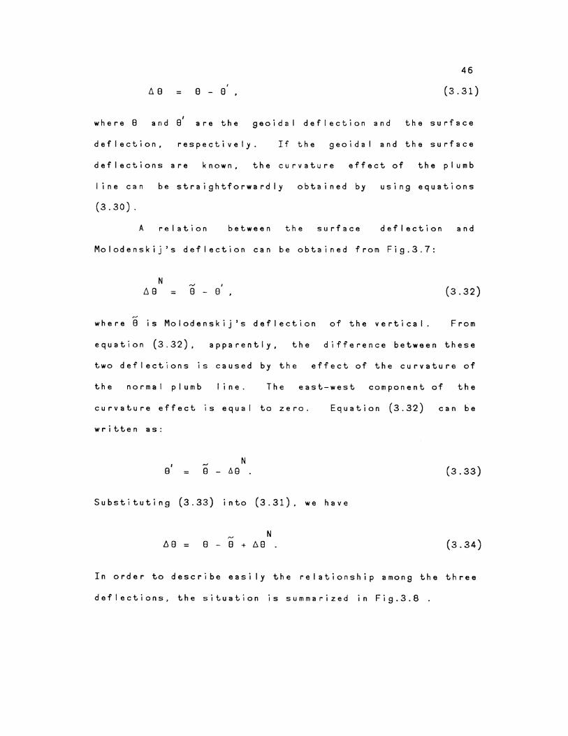
.b.a = a- e (3.31)

where 8 and a' are the geoidal deflection and the surface

deflection, respectively. If the geoidal and the surface

deflections are known, the curvature effect of the plumb

line can be straightforwardly obtained by using equations

(3.30).

A relation between the surface deflection and

Molodenskij 's deflection can be obtained from Fig.3.7:

"'

N ~8 =

I

8 - 8

where 8 is Molodenskij's deflection of the vertical.

(3.32)

From

equation (3.32), apparently, the difference between these

two deflections is caused by the effect of the curvature of

the normal plumb I in e. The east-west component of the

curvature effect is equal to zero. Equation (3.32)

written as:

I ,.., N

8 = 8 - tl8 .

Substituting (3.33) into (3.31). we have

N 68 = 8 - 8 + 68 .

can be

(3.33)

(3. 34)

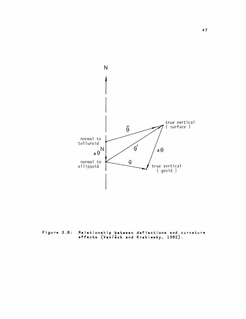
In order to describe easily the relationship among the three

deflections, the situation is summarized in Fig.3.8 .

normal to tell uroid

.o.8N

normal to ellipsoid

N

I true vertical ( surface )

true vertical ( geoid )

47

Figure 3.8: Rela~ionship between deflec~ions and curva~ure effec~s (Vanleck and Krakiwsky, 1982).

48

Obviously, if the geoidal deflection and

Molodenskij's deflection are available, the curvature effect

of the plumb line can be obtained by equations (3.34).

These deflections are obtained from Vening Meinesz's formula

and Molodenskij's formula. Due to the law of error

propagation, the errors of the geoidal deflection and of

Molodenskij's deflection will contribute to the errors of

the plumb line curvature effect at the computation point.

In addition, it is clearly uneconomical to compute the

geoidal deflection and Molodenskij's deflection separately.

The procedures for the calculation of the geoidal deflection

and Molodenskij's deflection are basic~lly the same.

instructive to compare them.

Referring to equations

difference between them is:

8-8 =\5}-{~J~ _1 JJ ( "' 4]( Ym lf

"? Y(

X

dS(I.)J)

dYJ

(3.1) and (3. 5).

[coso<}

Llg- AS- t.a )· . s t no<

·dV

It is

the

(3. 35)

From (3.3) and (3.4), the difference between the free-air

gravity anomaly on the geoid and the gravity anomaly on the

earth's surface is obtained from:

t. g -N = 0.3086·( H- H· ) (3.36)

49

where HN can be replaced by H·9/i, andY is the mean normal

gravity along the normal plumb line, given by (Heiskanen and

Moritz, 1967):

r = N

~o- 0.1543·H , (3.37)

where the factor 0.1543 is in mgal/m.

relation HN = H·9/Y into (3.36) yields

Substituting the

69 t~9 = 0.3086·H·( f- 9

) . '(

( 3. 38)

From (3.37) and (3.18) and setting the density p equal to

2.67g/cm~ the difference between the mean normal gravity~

and the mean gravity g is:

N g = ( '(o- 0.1543·H ) - ( g + 0.0424·H ) , (3.39)

or

r - g = - ( g + 0. 1967 · H - ro ) , (3.40)

where the factors 0.0424 and 0.1967 are also in mgal/m.

Because the Bouguer anomaly, denoted by ~g 8 is

defined as the difference between the Bouguer gravity g8 =

g+0.1967·H on the geoid and the normal gravity referred to

the elI ipsoid-- without taking into account the variation of

the actual topography -- (Heiskanen and Moritz, 1967), the

equation (3.40) can be written as:

(3.41)

Therefore, equation (3.38) becomes

50

1.!9- ~9 = (3.42)

The mean normal gravity Y can be replaced by the mean

gravity Ym o n t h e e I I i p so i d . The relative error of this

approximation is less than 17.. Substituting (3.42) into

(3.35). we obtain finally (Vanf~ek and Krakiwsky, 1982):

8 - 8 ={ ~ }-P}= :rr~. Jt ( o.3oas H h~:B + ~G l ·

X

d s (Y')

d\.jJ ·d.V + (3.43)

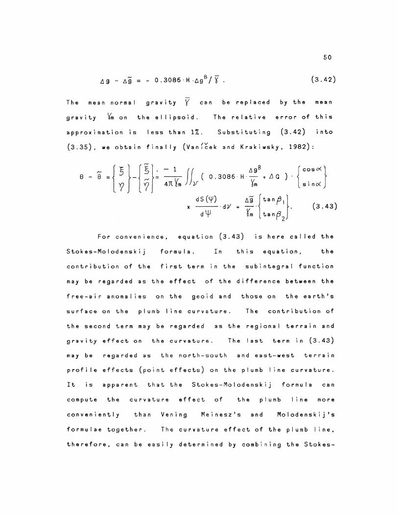
For convenience, equation (3.43) is here called the

Stokes-Molodenskij formula. In this equation, the

contribution of the first term in the subintegral function

may be regarded as the effect of the difference between the

free-air anomalies on the geoid and those on the earth's

surface on the plumb line curvature. The contribution of

the second term may be regarded as the regional terrain and

gravity effect on the curvature. The last term in (3.43)

may be regarded as the north-south and east-west terrain

profile effects (point effects) on the plumb I ine curvature.

It is apparent that the Stokes-Molodenskij formula can

compute the curvature effect of the plumb line more

conveniently than Vening Meinesz's and Molodenskij 's

formulae together. The curvature effect of the plumb I ine,

therefore, can be easily determined by combining the Stokes-

51

Molodenskij formula and the equation of the curvature effect

of the normal plumb I ine.

CHAPTER 4

PRACTICAL EVALUATION OF THE STOKES-MOLODENSKIJ FORMULA

4.1 I~IBQQ~~IIQ~

The Stokes-Molodenskij formula requires the knowledge

N of the gravity anomaly

...-A g. and the normal height H for the

solution of the terrain correction 6G at any point on the

surface of the earth. P r act i c a I I y , due to the d i s crete data

for t:,g and HN available, the formula (3.43) i5 evaluated as

summations. The small element dJf is replaced by an

appropriate area element (compartment or block). A mean

gravity anomaly and a mean normal height are necessarily

computed for each compartment or block. Since the

difference between the normal height and the orthometric

height is fairly small, usually it does not exceed 0.1 m

( ' .., Van1cek, 197 4) . In practice the former can be replaced by

the latter without affecting the accuracy of the value 6G.

for the computation of Stokes's integral, blocks of

various sizes bounded by geographical

30'x30', s'xs', and smaller are considered (Moritz, 1980b). In

the neighborhood of the computation point, it is proper to

use smaller blocks or compartments than for distant zones.

For the Vening Meinesz integral, such blocks of a few sizes

- 52 -

53

can also be used. Because Vening Meinesz's integral has a

stronger singularity than Stokes's integral, it requires

more detailed representation of ,.J

Ag and more rigorous

treatment around the computation point (Moritz, 1980b).

Obviously, the integral in the Stokes-Molodenskij formula is

similar to the Vening Meinesz integral so that the above

applies to it too.

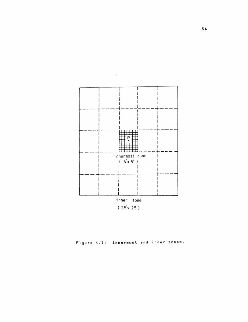
For the determination of the curvature effect of the

plumb line by means of the Stokes-Molodenskij formula 1n

this study, there are two different zones needed: innermost

and inner (Fig.4.1). The reason for neglecting outer zone

contribution to the curvature effect of the plumb I ine wi I I

be given later.

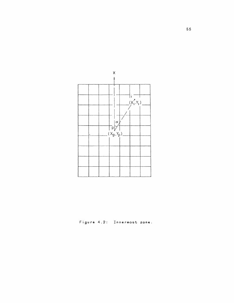
The innermost zone IS chosen to be enclosed by a

rectangle of the dimensions 9x7 km for ¢=45° (approximately

SxS minute rectangle). It consists of 63 lxl km blocks

(Fig.4.2). In the central block around the computation

point, circle-ring method is adopted for the centra I a rea

contribution. The outer radius is equal to 564 m chosen on

the basis of the same area as the central lxl km

compartment. The inner zone covers an area of a 25x25

minute block around the computation point, excluding the

innermost zone. It 1s subdivided into a few equal 5x5

minute cells. The choice of the boundary of the inner zone

is discussed 1n Section 4.6.

I I l I I I I I I I 1 I I I I I

"""- -- -t----l-- --:-----+----I I I I I I I I I I I I I I I I ----:-----.• -----:---~ I . I I I

-----1---- ----+-----1 innermost zone I I ( 5'x 5' ) I I I I I I I I I

----f-----------~----1 I I I

I I I I I 1 I I I J l I l

inner zone

( 25'x 25')

Figure 4.1: Innermost and inner zones.

54

55

X

! I

I

I ' (Xi .Yj) I -

1-~ 0(

p

( Xp.Yp)

Figure 4.2: Innermost zone.

56

I I

The choice of 5 x 5 blocks 1s based on the fact that

the mean gravity anomalies and the mean heights for these

blocks are readily avai I able. The data sets used for the

numerical evaluation of the Stokes-Molodenskij formula

include the point gravity anomalies, and the 5x5 minutes

mean gravity anomalies and mean heights. The mean heights

of 1x1 km blocks needed for the innermost zone are obtained

from the topographic maps at the scale 1:50,000.

In the Stokes-Molodenskij formula, if the orthometric

height is equal to 1000m, the first term 1n equation (3.43),

0.3086H·Lig 8 /~m, is about 10- 3 times smaller than the term t,g

in Vening Meinesz's formula, equation (3.1). Basi des,

orthometric heights of almost 727. of the points in the world

could be regarded as zero due to the fact that the about 727.

of global area is covered with water. The contribution of

the term to the plumb I ine curvature effect should be smal I.

In order to exemplify the above reasoning, a few points i n

New Brunswick (NB) have been tested. The contributions are

smaller than 0~001 everywhere. Therefore, the first term

can be neglected. It could be said that the term makes no

contribution to the curvature effect of the plumb I ine.

The numerical evaluation of the Stokes-Molodenskij

formula is. therefore, integrated by a summation over

discrete data:

57

- 1 d s (YJ) 6g ~-s = -I~c- ·coso< .!Jlf + Ym ·tanp,

4IT Ym d'f ( 4. 1)

- 1 d s ('f) ,....,

llg !JY( = -[ L1G· . s i no<.!JV + Ym. tan p2

4IT ~m dlV

and R2 H - H 3~

L1G ~ ·( .ag + -. :s) .fl)/, = 3 21( s 2R (4.2)

where H ts the mean height of the sma II compartment!::,)/, In

equation (4.2), if the height anomaly 5 is unknown, it may

be determined from sate I I ite potential coefficients, i . e.

Rapp 180 (Rapp, 1981). Because the value of 3't/2R is small

of 3·'t/2R·"S is (approximately 0.23 mgal/m), if the value

,-../

smaller than the error of the gravity anomaly 11g. this term

can be neglected. The height anomaly in the province of New

Brunswick, the tested area, approximately ranges from -1 m

to 2m (Merry, 1975).

0.5 mgal for 3'{/2R·S.

This gives values of order of -0.2 to

Then, equation (4.2) becomes

(4.3)

Due to the fast growing denominator tn equation

(4.3), the value of t!G will disappear very rapidly. For the

outside of the inner zone, the contribution of ~G IS

approximately equal to zero. A test of the contribution

wi II be given in Section 4.6.

58

Therefore, the summation in equation (4.1) can be

split into three parts, and the curvature effect components

of the plumb line are given by:

N ={)5 +L\5 +LJ5 + 1)5

1 2 3 =L\'Q +~'? +L\Y? .

1 2 3

(4. 4)

where .15 and .15 are the contributions of the innermost and 1 2

inner zones for the north-south component,

!J.Y( andL\Y( are the contributions of the innermost and 1 2

L\"5 and 3

inner zones for the east-west component,

tJ.'? are the 3

profile

north-south and the east-west terrain

contributions to the curvature effect

of the plumb line, respectively.

The terrain profile contributions are written as:

,..._, A9

= -·tan(3 ~m 1

Ll9 =-·tan~

'(m 2

(4.5)

N ~S is the north-south component of the curvature effect of

the normal plumb line.

59

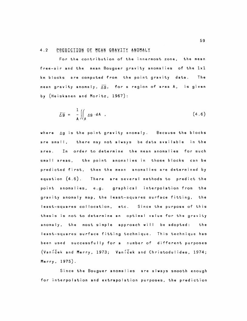
For the contribution of the innermost zone, the mean

free-air and the mean Bouguer gravity anomalies of the 1x1

km blocks are computed from the point gravity data. The

mean gravity anomaly, 6g, for a region of area A, is given

by (Heiskanen and Moritz, 1967):

(4.6)

where 6g is the point gravity anomaly. Because the blocks

are sma I I , there may not always be data available in the

area. In order to determine the mean anomalies for such

small areas, the point anomalies in those blocks can be

predicted first, then the mean anomalies are determined by

equation (4.6). There are several methods to predict the

point anomalies, e.g. graphical interpolation from the

gravity anomaly map, the least-squares surface fitting, the

least-squares collocation, etc. Since the purpose of this

thesis is not to determine an optimal value for the gravity

anomaly, the most simple approach wi I I be adopted: the

least-squares surface fitting technique. This technique has

been used successfully for a number of different purposes

( o'V

Van1cek and Merry, 1973; Vanf~ek and Christodulides, 1974;

Merry, 1975).

Since the Bouguer anomalies are always smooth enough

for interpolation and extrapolation purposes, the prediction

60

of free-air anomalies is often performed through the

intermediate step of Bouguer anomaly prediction (Si.inkel and

Kraiger, 1983).

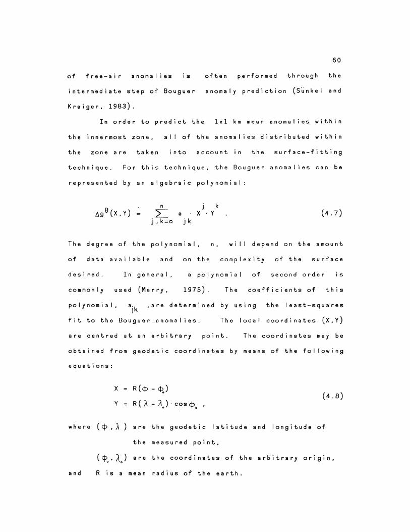
In order to predict the 1xl km mean anomalies within

the innermost zone, all of the anomalies distributed within

the zone are taken into account 1n the surface-fitting

technique. For this technique, the Bouguer anomalies can be

represented by an algebraic polynomial:

n

L:a j,k=o jk

j k X . y

The degree of the polynomial, n •

of data avai fable and on the

( 4. 7)

wi I I depend on the amount

complexity of the surface

desired. In general, a polynomial of second order IS

commonly used (Merry, 1975). The coefficients of this

polynomial, ajk ,are determined by using the least-squares

fit to the Bouguer anomalies. The local coordinates (X,Y)

are centred at an arbitrary point. The coordinates may be

obtained from geodetic coordinates by means of the following

equations:

X= R(¢-¢.) 0

Y = R (A - \) • COS ¢ 0

( 4. 8)

where (¢.A) are the geodetic latitude and longitude of

the measured point,

(<Po' A) are the coordinates of the arbitrary origin,

and R IS a mean radius of the earth.

61

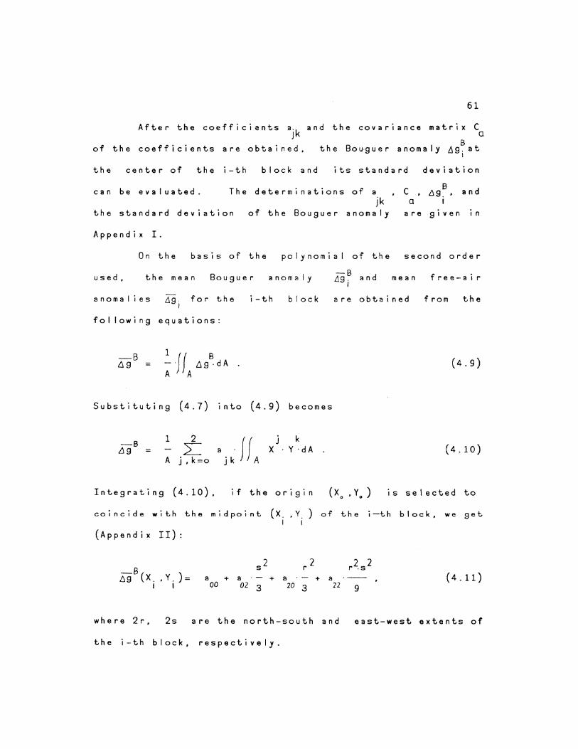
After the coefficients ajk and the covariance matrix C0

B o f t h e c o e f f i c i e n t s a r e o b t a i n e d , t h e B o u-g u e r a n om a I y l!g . a t

I

the center of the i-th block and its standard deviation

can be evaluated. The determinations of a . c B , ~g., and jk a 1

the standard deviation of the Bouguer anomaly are given in

AppendiK I.

On the basis of the polynomial of the second order

used, the mean Bouguer anomaly

anomalies L!g. for t.he I

following equations:

i-t.h block

-B 119. and I

mean free-air

are obtained from t.he

( 4. 9)

Subst.it.uting (4.7) into (4.9) becomes

-8 Ll 9 =

j k X · Y · dA (4.10)

Integrating (4.10). if the origin ( xo • y 0 ) IS selected to

coincide with the midpoint (X. • Y. ) of the i-th block, we get I I

(Appendix II):

f19B(X .• Y.)= 52 r2 r2.s2

a + a + a + a (4.11) I I 00 02 3 20 3 22 9

where 2r, 2s are the north-south and east-west extents of

the i-th block, respectively.

62

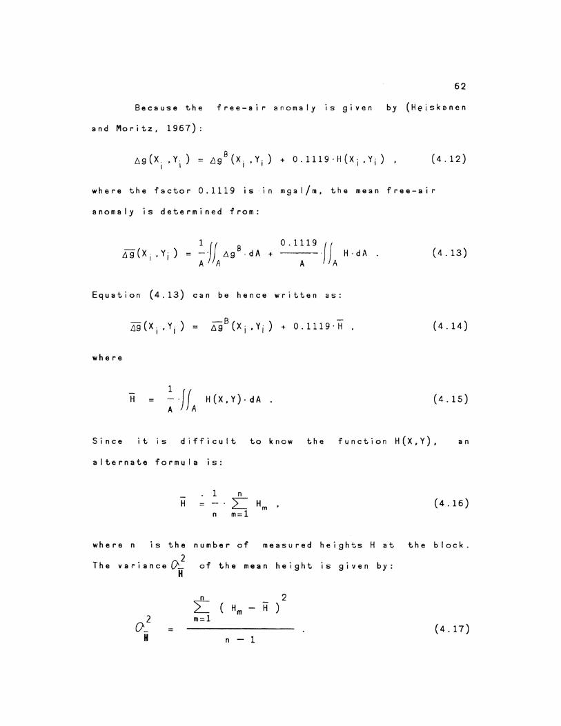
Because the free-air anomaly 1s given by (Heiskanen

and Moritz, 1967):

(4.12)

where the factor 0.1119 is in mgal/m, the mean free-air

anomaly is determined from:

1 J! + 0 .1Al19 ·JJA flg(Xi .Y;) = ~· A~g 8 ·dA H·dA .

Equation (4.13) can be hence written as:

where

-B -~g (Xi .Y;) + 0.1119·H

1 H = ~-IrA H(X,Y)·dA.

(4.13)

( 4. 14)

(4.15)

Since it 1s difficult to know the function H(X,Y), an

alternate formula is:

_ 1 n

H = L Hm (4.16) n m=1

where n is the number of measured heights H at the block.

The . 2 variance o_

H of the mean height is given by:

n 2 L ( H - H ) m

()_2 m=1 =

H n - 1 (4.17)

63

Equation (4.11) can be written in matrix form as:

-B 4g = b.a T

where

.! = ( a ' 00

a , 02

a , 20

and

b = 1, b = s2/3 , I 2

b = r 2/3 , 3

(4.18)

(4.19)

Then, applying the law of propagation of covariance

(Vanf~ek, 1980), the variance of ·.Ag 8 is obtained from:

2 O_s

..19

T = b. c . b a - (4.20)

Assuming that the mean Bouguer anomaly is uncorrelated with

the mean height, the variance of ~g is given by:

2 2 = ()'_ 8 + (0.1119·0_)

~g H (4.21)

In the vicinity of the computation point, Vening

Meinesz's function is approximated by (Heiskanen and Moritz,

1967):

dS('j')

dY-l =

2 -2 . 'f

(4.22)

The relative error of this approximation is about 1% for the

linear distance s=10 km from the computation point, and

about 3% for s=30 km (ibid., p.121). Within the small

64

spherical distance~ (corresponding to a linear distance of

a few kilometres), we may regard the sphere as a plane,

where~ is given by:

'-\} ; s/R (4.23)

Substituting (4.23) into (4.22) yields:

d s (If) 2R 2

= -2- (4.24) dlf./ s

The so I i d angle element d.V 1n the rectangular

coordinate system and 1n the polar coordinate system are

written respectively as:

dlf = dx·dy

R2 (4.25)

and S · d S· do(

d.lf = R2

(4.26)

Substituting (4.24) and (4.25) into (3.43), the contribution

of the innermost zone to the curvature effect components is:

- 1 ff -2 R 2 d X • d y = -- /:)G ·--2- ·coso<. · 2

41t ~m A1 s R

- 1 JJ -2R 2 ll '?, = -- D.G · --2- · s i n o<.

47t ~m A1 s

dx.dy

R2

Rearranging (4.27) yields:

115 1

(4.27)

(4.28)

65

and (cf. equation (3.6))

~G- - 1-j'( H -Hp · .1g·dx·dy , - 2 7( }t.A s 3

I

(4.29)

where .1A 1 is the area of the lx1 km block inside the

innermost zone. Therefore, the part of equation ( 4. 1)

pertinent to the innermost zone is given by:

and

1151,1 = nl 6X · 4Y

L ~G ·cos£X·( 2 ) i=1 s

nl

L .6G i=l

!:>X· ~:>y

sind.·( 2 ) s

1 t.x . tJ.y .1G = - ·( H

27l H ) · Ag · ( 3 )

p s

I::. A I = /:; X . ll y •

(4.30)

(4.31)

(4.32)

where n1 IS the number of lxl km blocks used,

H. IS the mean value of the height in the i-th block, I

t,g. i s the me an v a I u e i n the i - t h b I o c k of the I

free-air anomaly,

~i is the azimuth of the I ine connecting the computa-

tion point and the midpoint of the i-th block,

CIX = 6 y = 1 k m ,

s is the distance between the computation point and

the midpoint of the i-th block, and

~., s are given by: I

o(.= arctan( I

y.- y I p )

66

( 4. 33)

(4.34)

where (XP,YP) are the coordinates of the computation point,

and (X; ,Y;) are the coordinates of- the midpoint of the i-th

block in a local plane coordinate system (Fig.4.2).

For the lxl km blocks near the computation point, in

equations (4.30), it is not accurate enough to evaluate the

values of t.x·Ay/s 2 and t.X·t.y/s3 at the center of each block.

A more rigorous approach is to integrate over the block.

Setting C=l:lx-t:.y/s2 and D=AX·I:ly/s3, the more proper values of C

and Dare given by:

C = -1-jf C ·dA

LIA I AA,

D = - 1-j( D·dA b. A I }llA I

(4.35)

where C and D denote the mean values of C and D for the

block, and tlA 1 is the block area.

The error in the numerical integration 1s I I ustrated

in Table 4.1.

For those blocks within a rectangular region of the

dimensions 7x7 km, centred on the computation point, the

mean values (4.35) are used. The relative error IS thus

kept below 1.8X for C and 4X for D.

67

TABLE 4.1

The differences between the values C and D and their mean values.

- -dist. c c error D D error

(s) ( 7. ) ( 7. ) 1 km 1. OOE+O 1.16E+0 13.9 l.OOE-3 1. 40E-3 28.7

2 km 2.50E-l 2.60E-l 4.0 1. 25E-4 1.37E-4 8.8

3 km l.llE-1 1.13E-l 1.8 3.70E-5 3.86E-5 4.0

4 km 6.25E-2 6.31E-2 1.0 1.56E-5 1.60E-5 2.3

5 km 4.00E-2 4.03E-2 0.7 8.00E-6 8.12E-5 1.5

For the central block where the computation point

lies, since the midpoint of the block coincides with the

computation point, equations (4.30) cannot be used to

evaluate the contribution of the central block. For this

reason, the circular-ring method is adopted. In this study,

there are three rings used whose radii are lOOm, 200m, and

564m (Fig.4.3). The outer radius is chosen on the basis of

the same area as the central compartment, therefore the

total area of 4 corners is equal to the total area of 4

overlaps (Fig.4.3). It is assumed that the contributions of

the corners and the overlaps are balanced out.

Substituting (4.24) and (4.26) into (3.43), we obtain

- 1 Jf -2 R 2 s . d s · do< L1 S = -- .6G · --2- ·coso<

1 4KYm A2 s R2 2 (4.36)

- 1 Jf -2R s. d s · do< ~:.YI = -- f1G.--2-·sino<

( 1 4 7( rm A 2 s R 2

68

N

Sz

and

t.G s·ds·do<

. Ll g. ---::-­R2

where A2 1s the central block area, and

69

(4.37)

!::.A 2 1s the area of the circular-ring compartment.

Rearranging equations (4.36) and (4.37), we obtain

<15 1

and

1 JJ coso< ---- hG · ---·ds. d~ 2 7t ~m A 2 s

s i no(

· --- ·dS· do( s

· .1g· ds ·do<. .

(4.38)

(4.39)

Then performing these integrations, the contribution of the

central block is given by (Appendix III):

and

1 m

11512 = -v ·L 27COm j=l

1 m

tJ'? , '2

= ·L 2J\~m j =1

1

llG_-(sino< 2 -sino< 1 ) ·ln(s2 /s 1 )

J

hG ·(coso<.- coso< 2 ) ·In (s /s 1 ) · I 2 J

1 1 = --·(o<-o<.) ·(H- H )·.1g·(

2TC 2 I j p j .1G )

j s I

where H. rs the mean height of the j-th compartment, J

(4.40)

(4.41)

o< 1 , o< 2 are the azimuths of two edges of the compartment,

respectively, and o<. >o< (Fig.4.4), 2 I

s 1 , s 2 are the inner and outer radii,

Llg. is the mean free-air anomaly, and J

70

m IS the number of the compartments used (within the

circular rings).

Finally, the total c-ontribution of the innermost zone

is obtained from:

(4.42)

The inner zone, composed of a number of SxS minutes

blocks, covers an area of a 25x25 minute geographic

rectangle, excluding the innermost zone. Analogous to

(4.30) and (4.31), the contribution of the inner zone can be

written as (cf. equation 4.1):

lls - 1 n2 d s (41) =

4](rm L:: .6G ( ) ·cos¢· coso(· .6Cl:>·llA

2 i=1 d 41 i i i

dS (4J) ( 4. 43)

- 1 n2 l1'f( =

4n:Ym L l!G ( ) · cos<):>· s i no(· Llc):>·L\A

2 i=1 d'-P

and

R2 (H;- Hp) fiG = 3 .6.g cos<):> · Ll <P · .6/\ (4.44)

21( s

s = 2Rsin(~/2) . (4.45)

I I

where n2 is the number of SxS blocks used,

¢. I

is the latitude of the midpoint of the i-th block,

ll<P = .1A = s' ,

71

and the other symbols have the same meaning as before.

In the a b o v e e quat i on s , \fli , o(; a r e g i v en by :

If· =arccos( sin¢· sin¢. + cos¢.cos¢.·cos(J.. -AP) ) I p I p I I

(4.46)

cos¢isin(;.\;-Ap) ), o<.; =arctan(

cos¢· s i n<f>. - s i n<j) ·cos<f>.·cos (A.- :A. ) p I p I I p

(4.47)

where (<:pp./\p) are the geodetic coordinates of the

computation point, and (<:pi ,,Ai) are the geodetic coordinates

of the midpoint of the i-th block.

Due to the rapid change in Vening Meinesz's function,

it should be treated rigorously

dS(\fJ)

dYl = (4.48)

where dS(4J)/dlf denotes the mean value of dS(yJ)/dljJ for the

block, and A is the block area. For those blocks whose

spherical distance from the computation point is smaller

than o:s, the value of dS(\fJ)/d~ is replaced by the mean

value of dS(~)/d~ (Merry, 1975).

Analogously, the mean value of R 2 -cos¢>·~d:>·LIA/s 3 in

(4.44) is given by:

2 1 j~ R ·cos¢ ·t.¢·AA

E = - ·dA 4A ~A s 3

(4.49)

where is the s'xs' block are a.

equation (4.49) may be written as:

72

E =JJ ~-dA tJA s

( 4. so)

Equation (4.SO) 1s used when the spherical distance of those

blocks is smaller than 1s'. The relative error wi I I be below

4%.

The terrain profile contribution to the components of

the curvature effect are given by equation (4.S). These can

attain large values in steep mountains. For the terrain

profile contribution, sometimes the uncertainties of the

terrain inc I ination wi II give large error for the curvature.

For the sma I I terrain inc I ination, between 0° and 2s: the

error of 1o in (3 value wi II give the error of 0~004/mgal for

the plumb I ine curvature effect. For instance, when the

free-air anomaly is SO mgals, the error of the curvature

effect is 0!'2. No matter how the terrain inclinations are

measured, either from topographic maps or from field works,

the evaluation of the inclinations should be performed

carefully.

4.S.1

The evaluation of terrain slope can be done simply.

Let the north-south (or east-west) terrain profile be a

function of horizontal coordinate x (or y) . Then we may

write the north-south and east-west terrain profiles,

denoted by H(x) and H(y) respectively:

where c. I

u H ( )() = L c

i=O

u H (y) = ~ d

i=O

d. are some I

coefficients, and (x,y)

73

• X

(4.51)

. y

coefficients, u is the number of

are the coordinates referred to the

local system, whose origin coincides with the computation

point P. Measuring the heights H(x) and H(y) for several

values K andy, the coefficients c. I

can be determined

using the I east-squares procedure. The north-south and

east-west terrain slopes are given by the coefficients c1 and

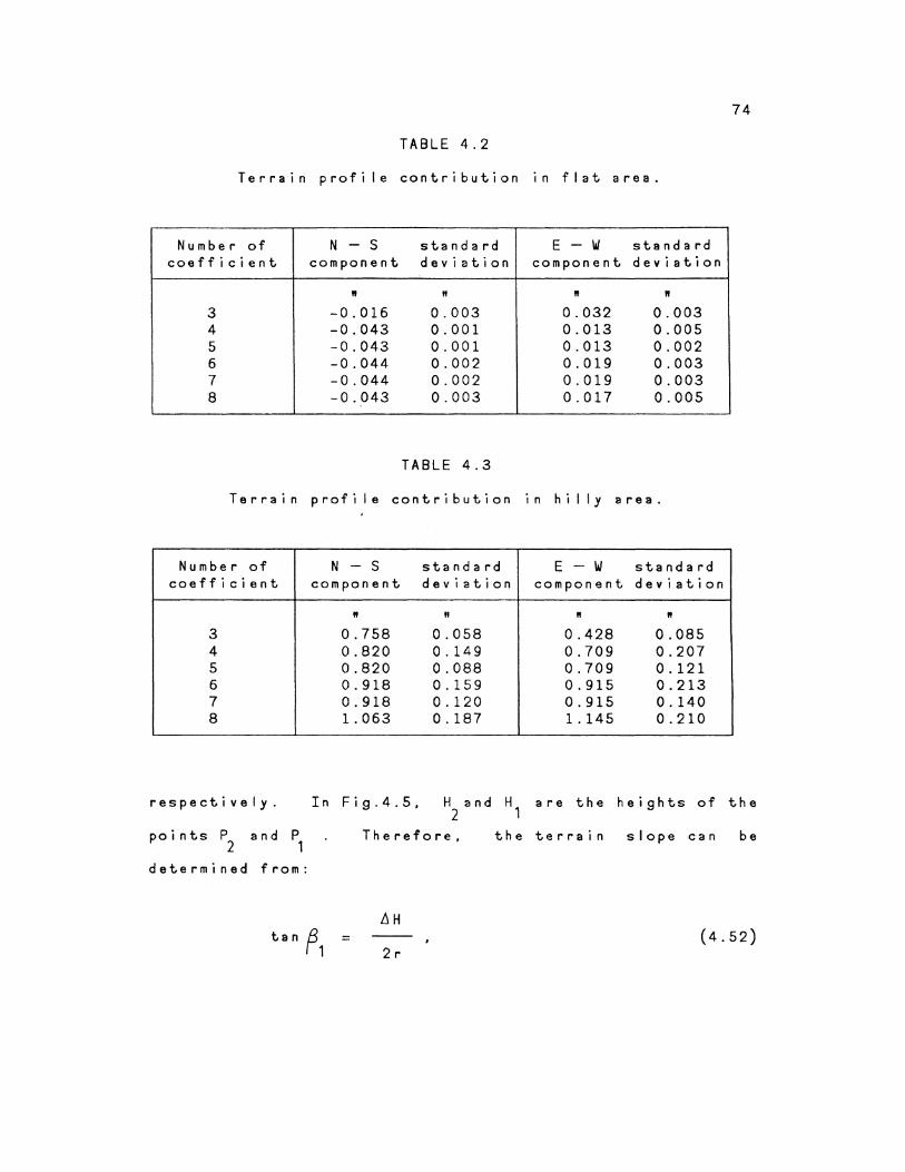
This simple model has been tested 1 n two different

kinds of areas, flat and hilly. Twenty one data for each

profile are measured at the following coordinates: -250m,

-200m, . . . . , 200m, 250m, 1n 25m interval . The results are

shown in Tables 4.2 and 4.3. As can be seen, the number of

the coefficients does not make significant difference for

the terrain profile contribution in flat area. However, the

significant difference is demonstrated 1n hilly area. In

this case, the choice of the number of the coefficients

comes into question.

Therefore, another approach to estimate the terrain

slope is developed. Fig.4.5 shows the north-south terrain

profile at the computation point. Let us choose points P2

to be north and south of the computation point P,

74

TABLE 4.2

Terrain profile contribution 1n flat area.

Number of N - s standard E - w standard coefficient component deviation component deviation

" It " " 3 -0.016 0.003 0.032 0.003 4 -0.043 0.001 0.013 0.005 5 -0.043 0.001 0.013 0.002 6 -0.044 0.002 0.019 0.003 7 -0.044 0.002 0.019 0.003 8 -0.043 0.003 0.017 0.005

TABLE 4.3

Terrain profile contribution 1n hilly area.

Number of N - s standard E - w standard coefficient component deviation component deviation

" " " " 3 0.758 0.058 0.428 0.085 4 0.820 0.149 0.709 0.207 5 0.820 0.088 0.709 0.121 6 0.918 0.159 0.915 0.213 7 0.918 0.120 0.915 0. 140 8 1.063 0.187 1.145 0.210

respectively. In Fig.4.5, H and H are the heights of the 2 1

p o i n t s P 2 a n d P1

determined from:

Therefore, the terrain slope can be

i}H tan p1 = (4.52)

2r

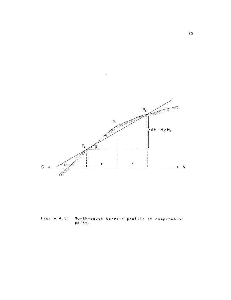
s

Figure 4.5:

N

North-south terrain profile at computation point.

75

76

where r is the distance from the computation point P. Then

the terrain profile contribution to the curvature effect of

the plumb line is determined using (4.52) and (4.5). Since

the tangent of {3 is a very localized parameter, if we choose 1

10 different values of rand compute the terrain slopes and

the curvature effects, the results are different (Tables 4.4

and 4.5). In flat area, maximum difference between the

curvature effects determined from different distances is

about 0~015 (Table 4.4). In hilly area, maximum difference

reaches about 1~2 (Table 4.5). In this case, it may be

necessary that the the least-squares approximation be used

to find a trend for the terrain slope.

In order to determine a trend for the terrain slope,

the terrain slope tanp1 can be represented by an algebraic

polynomial of r:

tan p ( r) = 1

2

?= a . r 1=0

where a. are some coefficients. I

( 4. 53)

The coefficients can be

determined using the least-squares approximation. When the

distance r approaches to zero,

estimated value for the terrain

computation (Fig.4.6).

the coefficient a 0

is the

slope at the point of

For the determination of the coefficients and

covariance matrix of the coefficients see Appendix I. The

variance of tanf1 is equal to o-2 . a

0

The determination of the

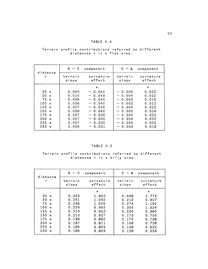
TABLE 4.4

Terrain profile contributions referred to different distances r in a flat area.

N - s component E - Ill component distance

r terrain curvature terrain curvature slope effect slope effect

" " 25 m 0.009 - 0.044 - 0.004 0.022 50 m 0.010 - 0.049 - 0.004 0.022 75 m 0.008 - 0.040 - 0.003 0.016

100 m 0.008 - 0.040 - 0.002 0.012 125 m 0.007 - 0.035 - 0.004 0.022 150 m 0.008 - 0.040 - 0.005 0.024 175 m 0.007 - 0.035 - 0.004 0.022 200 m 0.007 - 0.035 - 0.004 0.022 225 m 0.007 - 0.035 - 0.004 0.022 250 m 0.006 - 0.031 - 0.003 0.016

TABLE 4.5

Terrain profile contributions referred to different distances r in a hilly area.

N - s component E - Ill component distance

r terrain curvature terrain curvature slope effect slope effect

" " 25 m 0.323 1.403 0.408 1.774 50 m 0.251 1.092 0.213 0.927 75 m 0.236 1.026 0.274 1.192

100 m 0.229 0.993 0.305 1.324 125 m 0.219 0.953 0.226 0.980 150 m 0.213 0.927 0. 173 0.750 175 m 0.198 0.860 0. 170 0.738 200 m 0. 187 0.811 0. 168 0.728 225 m 0. 186 0.809 0. 148 0.632 250 m 0. 186 0.809 0. 128 0.556

77

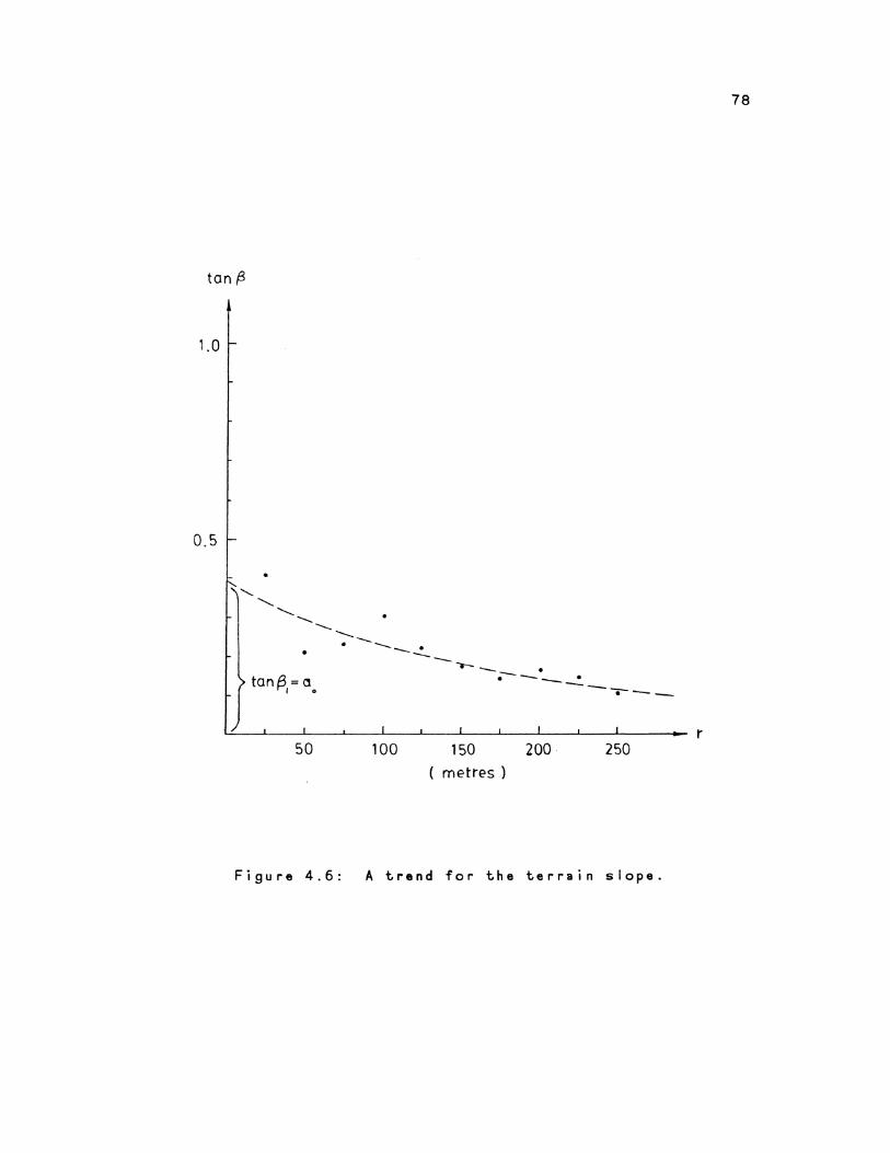
tan ,B

1.0

0.5

........ ...........

........... ...........

...........

•

tan{3 = o I o

50

............ ___ -- . ----

100

.......... _ . . --- ---- ---~ -------150

metres ) 200 250

Figure 4.6: A trend for the terrain slope.

78

r

79

east-west terrain inclination follows the same computational

procedures as that of the north-south.

4.6 ZQ~~ ~Q~~Q~BX EQB Itl~ ~Q~IBI~~IIQ~ QE Itl~ B~9IQ~~b I~BB~I~ ~~Q 9B~~IIX ~EE~~I~

It has been already stated tn Section 4.1 that the

value of AG disapears very rapidly with distance because of

the fast growing denominator in the subintegral function.

Thus, the integration does not have to be carried out very

far.

In order to determine zone boundary for the

contribution of ~G (regional terrain and gravity effect) the I I

variation of the geographic rectangle ranges from 15x15 to

I tn 10 increments. Computing the contributions of

the values 6G to the curvature effect and their RMS and

0 I 0 I

taking the values of 105x105 as standard, the differences in

the curvature effects and the RMS from the standards are

shown in Fig.4.7. The tested area is chosen in a hilly area

whose heights range from 15m to 480m. From the figure, a

conspicuous change in the differences occurs on

this graph: it appears that the contribution of ~G to the

curvature effect of the plumb line converges at this size of

the zone. The contribution coming from the value 6G may be

regarded as the regional terrain and gravity effect on the

curvature of the plumb I in e, Consequently, it can be

concluded that topography and gravity outside the above zone

make no effect.

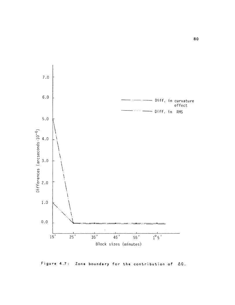
<::t-I 0 ....... Vl

" c 0 u Q) Vl u !.. <U

Vl Q)

u c Q)

!.. Q)

4--4-·.--0

7.0

6.0

5.0

4.0 \

\ \

3.0

2.0

1.0

0.0

15'

\ \

\ \

"'-\

80

Diff. in curvature effect

-- · · · -- Diff. in RMS

·~,,...,...-_,___~-:-:-.'-=" ~

25' 35' 45' 55 I

Block sizes (minutes)

Figure 4.7: Zone boundary for the contribution of ~Q.

81

In order to examine the reliability of the results,

the accuracy of the curvature effect of the plumb line has

to be estimated. The uncertainties of the plumb I in e

curvature effect are propagated from the errors of the

gravity anomalies and the heights. The gravity anomalies

are correlated with each other as a function of distance

(Heiskanen and Moritz, 1967) . The representation of this

correlation can be carried out empirically (Lachapelle and

Schwarz, 1980). The mean gravity anomalies are also

correlated with each other. In this thesis, for the

accuracy estimation of the curvature effect, the mean

gravity anomalies are assumed to be uncorrelated. On the

basis of this assumption, from equations (4.4), the standard

deviations of the components of the curvature effect are

determined from:

)c 2 2 2 0.15 1?'.15 + 0'65 + 0.15 )

1 2 3 (4.54)

06'9 Jc o-~?, 2 2 ) = + {)'A? + O'~.r;

2 3

and the var1ances of the curvature components of the

innermost zone are obtained from:

2 2 2

~5 = ()<15 + 0.15 2 1 2 1,1 2 1,2 (4.55)

0~'7. = O'Ll'? + (/'AY(

1 1,1 1, 2

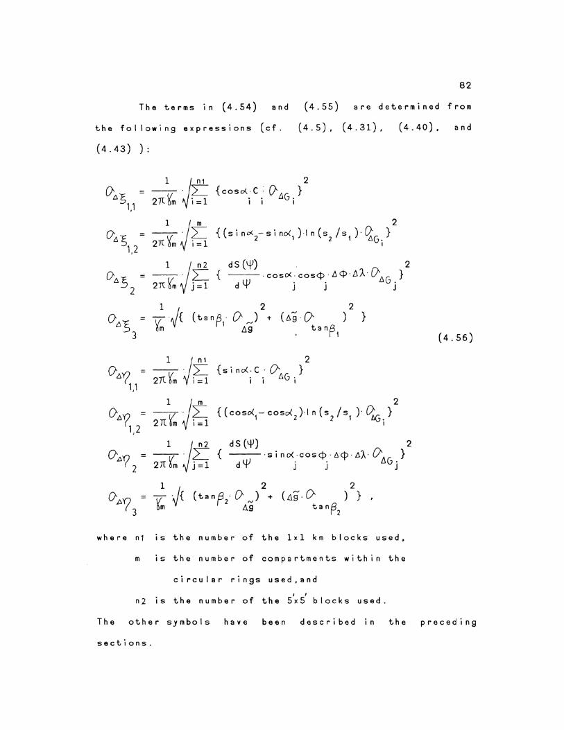
82

The terms in (4.54) and (4.55) are determined from

the following expressions (cf. (4.5), (4.31), (4.40), and

(4.43) ):

1 f' 2

()-LIS = -·L {coso<.·C: ()- llG. } 1,1

27l ~m i =1 i i I

1 j m 2

0'.15 = -·L: {(si no<. 2-si no( 1 )·1 n (s 2 /s 1 )·~G-} 2/l tm i =1

1,2 I

2 1 j n1 0 =-·~ Ll'?1,1 27l~m i=1

{sino<·C·D' } i i I1G i

-·~ 1 j m

27L~ i=1

2 { (coso<1- coso< 2 )·1 n (s 2 /s 1 )· qG.}

I

1 J n 2 d S (Yl) 2 OLI'? = --· L { ·sino<·cos¢·6<f>·LlA·O' }

2rr v . 1 d''J . . !JG-2 om J = 't' J J J

1 2 2 O.LID = - ·J{ (tanp2· 0 ,J + (49· 0 ) } ,

( 3 (m A9 tan~2

where n1 IS the number of the 1x1 km blocks used,

m 1s the number of compartments within the

circular rings used,and

I I

n2 is the number of the 5x5 blocks used.

(4.56)

The other symbols have been described in the preceding

sections.

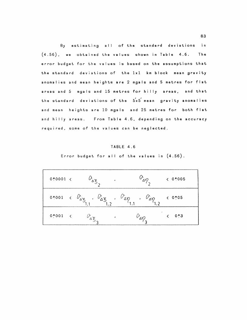
83

By estimating all of the standard deviations in

(4.56). we obtained the values shown in Table 4.6. The

error budget for the values is based on the assumptions that

the standard deviations of the 1x1 km block mean gravity

anomalies and mean heights are 2 mgals and 5 metres for flat

areas and 5 mga Is and 15 metres for hilly areas, and that

the standard I I

deviations of the SxS mean gravity anomalies

and mean heights are 10 mgals and 25 metres for both flat

and hilly areas. From Table 4.6, depending on the accuracy

required, some of the values can be neglected.

TABLE 4.6

Error budget for all of the values 1n (4.56).

0~0001 < {)L\5 . o-41 < 0~005 2 2

0~001 < 0;,5 . ~5 , ()-tl'? , O'll1. < 0~05 1,1 1,2 1.1 1. 2

0~001 < 0Ll5 , ()~:>'9 < 0~3

3 3

CHAPTER 5

COMPUTATIONAL RESULTS AND COMPARISONS

Six

Brunswick

test stations

(Fig.5.1) have

located in the province of New

been selected for this thesis.

Their geodetic coordinates and elevations are shown in

Tables 5.1 through 5.6. Two of them, stations 2 and 3, lie

in mountainous areas, the rest in flat areas.

In Tables 5.1 through 5.6, the results are shown from

the technique based on

Molodenskij 's approaches.

the combination of Stokes's and

above. For convenience,

The data used have been described

the curvature effect of the plumb

line obtained from the Stokes-Molodenskij formula is here

ca I I ed the ~!!Qk~§=~Q!Qg~fl§kll £!!.!::!~!!!!.!:~ ~ff~£!!, abbreviated

by S-M. In the Tables, the first two rows show the

contributions of AG of the innermost and inner zones. Row 3

shows the terrain profile contributions. The meanings of

the rest of the

Tables.

rows can be easily

The contributions of ~G are

areas than in flat areas. The

interpreted from the

larger 1n mountainous

maximum value for the

contributions is 0~1 in alI of the tested points. Among the

contributions, the terrain profile contributions along the

- 84 -

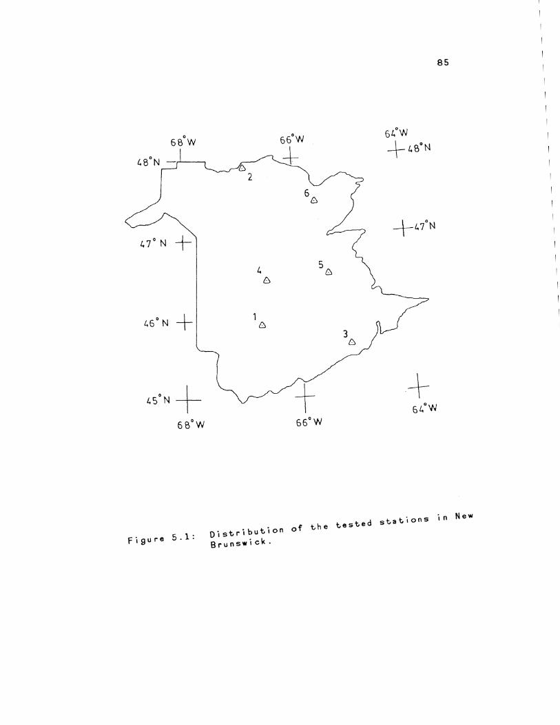
85

0

68 w

t. 7° N + +47°N

L. 5 [)

[)

1.6° N + 1 [)

3 [)

t. 5o N + t + 64°W

68"W 66"W

f;S"'e S.lo o;sc,;b,c;o" of che CesCed scoc;o"s '" N•• Brunswick.

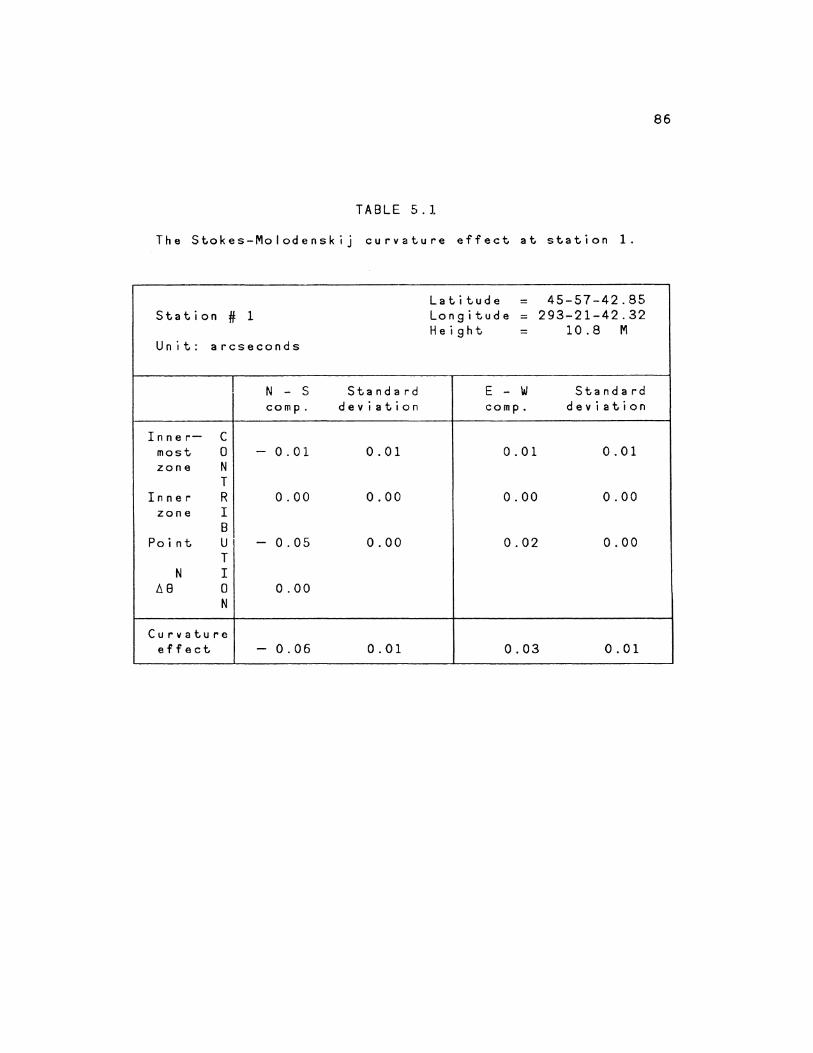
86

TABLE 5.1

The Stokes-Molodenskij curvature effect at station 1.

Latitude = 45-57-42.85 Station # 1 Longitude = 293-21-42.32

Height = 10.8 M Unit: arcseconds

N - s Standard E - w Standard comp. deviation comp. deviation

Inner- c most 0 - 0.01 0.01 0.01 0.01 zone N

T Inner R 0.00 0.00 0.00 0.00

zone I 8

Point u - 0.05 0.00 0.02 0.00 T

N I ll8 0 0.00

N

Curvature effect - 0.06 0.01 0.03 0.01

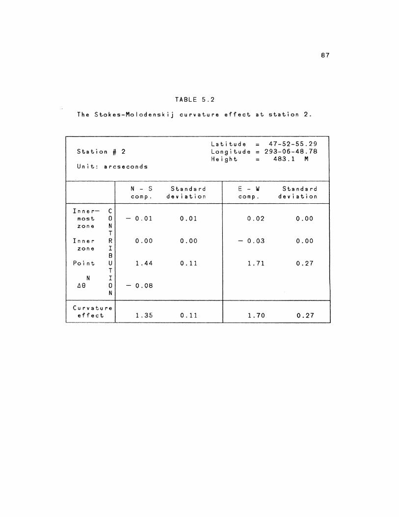
87

TABLE 5.2

The Stokes-Molodenskij curvature effect at station 2.

Latitude = 47-52-55.29 Station # 2 Longitude = 293-06-48.78

Height = 483.1 M Unit: arcseconds

N - s Standard E - w Standard camp. deviation camp. deviation

Inner- c most 0 - 0.01 0.01 0.02 0.00 zone N

T Inner R 0.00 0.00 - 0. 03 0.00

zone I B

Point u 1. 44 0. 11 1. 71 0.27 T

N I ~8 0 - 0.08

N

Curvature effect 1.35 0.11 1. 70 0.27

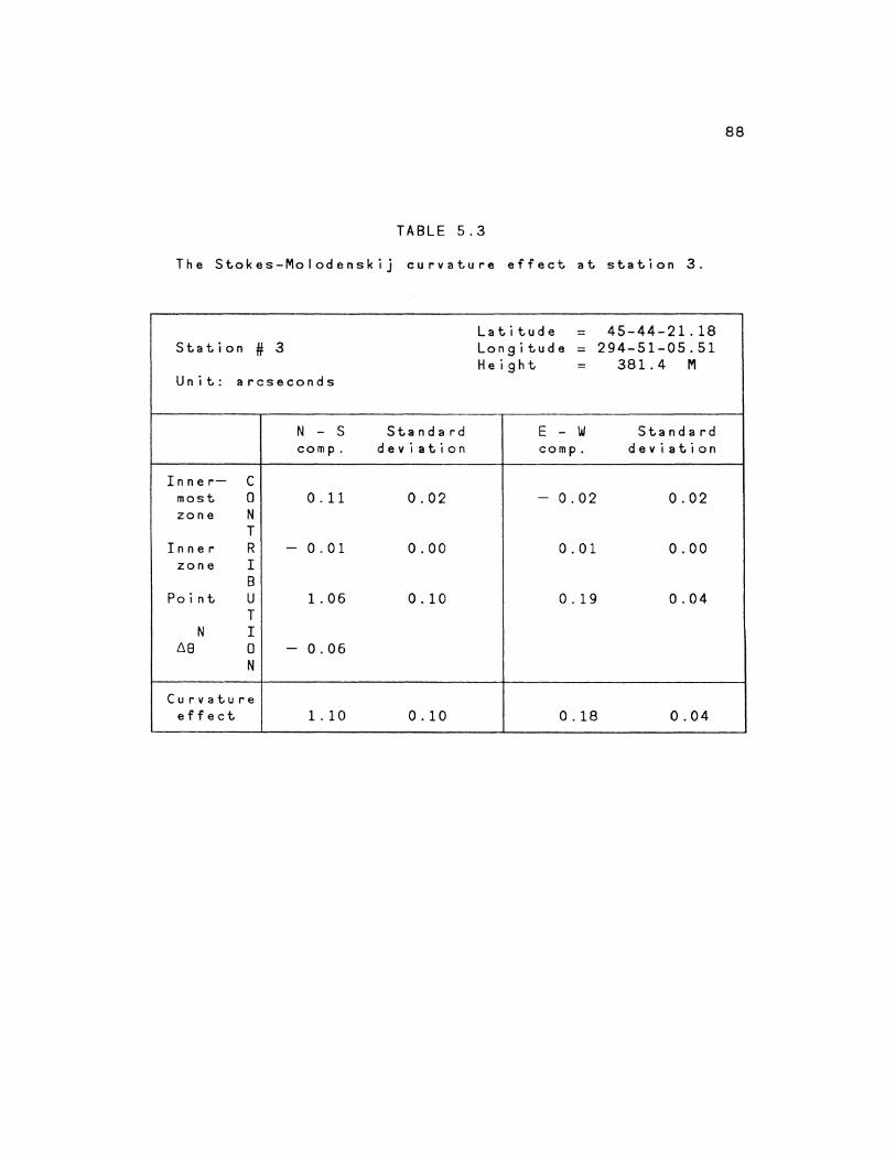
88

TABLE 5.3

The Stokes-Molodenskij curvature effect at station 3.

Latitude = 45-44-21.18 Station # 3 Longitude = 294-51-05.51

Height = 381.4 M Unit: arcseconds

N - s Standard E - w Standard comp. deviation comp. deviation

Inner- c most 0 0.11 0.02 - 0.02 0.02 zone N

T Inner R - 0.01 0.00 0.01 0.00

zone I B

Point u 1.06 0.10 0.19 0.04 T

N I .0.8 0 - 0.06

N

Curvature effect 1. 10 0.10 0.18 0.04

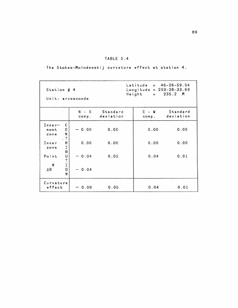
89

TABLE 5.4

The Stokes-Molodenskij curvature effect at station 4.

Latitude = 46-26-59.54 Station # 4 Longitude = 293-28-33.69

Height = 235.2 M Unit: arcseconds

N - s Standard E - w Standard comp. deviation comp. deviation

Inner- c most 0 - 0.00 0.00 0.00 0.00 zone N

T Inner R 0.00 0.00 0.00 0.00

zone I 8

Point u - 0.04 0.05 0.04 0.01 T

N I 118 0 - 0.04

N

Curvature effect - 0.08 0.05 0.04 0.01

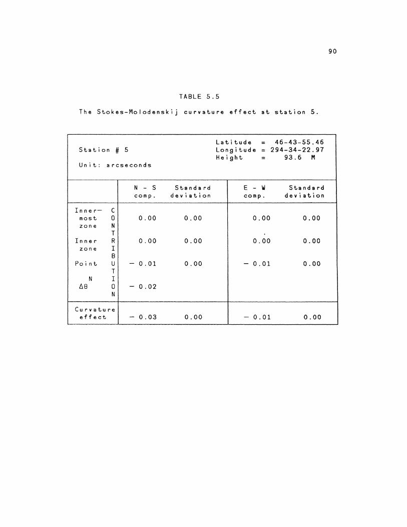
90

TABLE 5.5

The Stokes-Molodenskij curvature effect at station 5.

Latitude = 46-43-55.46 Station I# 5 Longitude = 294-34-22.97

Height = 93.6 M Unit: arcseconds

N - s Standard E - 1M Standard comp. deviation comp. deviation

Inner- c most 0 0.00 0.00 0.00 0.00 zone N

T . Inner R 0.00 0.00 0.00 0.00

zone I 8

Point u - 0.01 0.00 - 0.01 0.00 T

N I 68 0 - 0.02

N

Curvature effect - 0.03 0.00 - 0.01 0.00

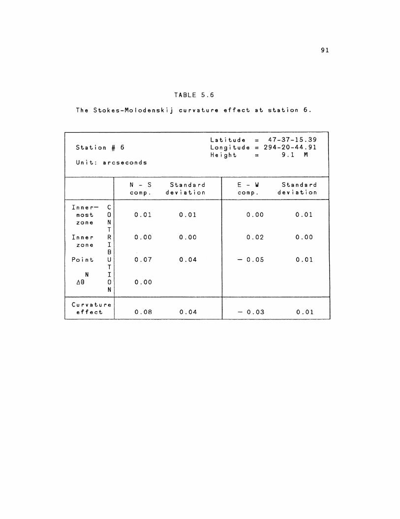
91

TABLE 5.6

The Stokes-Molodenskij curvature effect at station 6.

Latitude = 47-37-15.39 Station # 6 Longitude = 294-20-44.91

Height = 9.1 M Unit: arcseconds

N - s Standard E - w Standard comp. deviation comp. deviation

Inner- c most 0 0.01 0.01 0.00 0.01 zone N

T Inner R 0.00 0.00 0.02 0.00

zone I 8

Point u 0.07 0.04 - 0.05 0.01 T

N I LIS 0 0.00

N

Curvature effect 0.08 0.04 - 0.03 0.01

92

north-south and the east-west directions are a lot larger

than the others. The east-west terrain profile contribution

to the plumb I ine curvature effect reaches about 1~7 (at

station 2).

5.2 ~Q~E~BI~Q~~ e~IW~~~ I~~ ~IQ~~~=~QbQ~~~~~!4 ~~Q I~~ ~~IBQ=QB~~I~~IBI~ ~~B~~I~B~ ~EE~~I~.

Equation (3.27) indicates that if the geoidal and the

surface deflections (or astra-geodetic deflection) are

known, then the curvature effect of the plumb line can be

determined. For convenience, the curvature effect of the

plumb I ine obtained from the difference between the geoidal

deflection and the surface deflection is here called the

Both the surface and geoidal deflections are

available for the tested points. The geoidal deflections

are predicted by program ODOVE, written by Lachapelle (Table

5. 7); the surface deflections (Canadian Astra-geodetic

deflections, 1981) are avai I able from Geodetic Survey of

Canada. If the surface deflections and the geoidal

deflections are referred to different ellipsoids, this two

kinds of deflections must be brought into the same system.

That must be done before determining the curvature effect.

The surface deflections refer to a geocentric

ellipsoid with parameters (F.Faucher, personal

communication, 1984):

a = 6378135 metres

1/f = 298.257

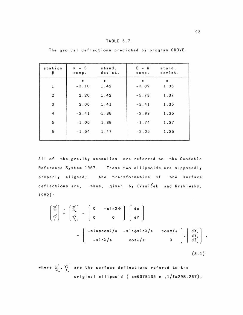
93

TABLE 5.7

The geoidal deflections predicted by program GDOVE.

station N - s stand. E - Ill stand. # comp. deviat. comp. deviat.

II II II II

1 -3.10 1. 42 -3.89 l. 35

2 2.20 1.42 -5.73 1. 37

3 2.06 1. 41 -3.41 1. 35

4 -2.41 ·1. 38 -2.99 1. 36

5 -1.06 1. 38 -1.74 1. 37

6 -1.64 1. 47 -2.05 1. 35

All of the gravity anomalies are referred to the Geodetic

Reference System 1967. These two elI ipsoids are supposedly

properly aligned; the transformation of the surface

deflections are, thus, given by (Vanf~ek and Krakiwsky,

1982) :

[;.]~[~] [: -sin2<!>

0

+ [ -sin<Pcos!./a

-si n?o./a

]· [ :: l -sinct>sin!./a cos<P/a l [ cost../a 0

I I

where S, 1 are the surface deflections refered to the 0 0

( 5. 1)

original ellipsoid ( a=6378135 m .1/f=298.257),

94

da, df are the differences in the size and shape of

the e IIi psoids (The parameters of CRS67 minus

those of the original ellipsoid), and

dX., dYo, and dZ. are the differences of the coordinates

of the ellipsoid center with respect to the center

of mass of the earth (The coordinates of CRS67

minus those of the original). Here dX =dY :dZ =0. 0 0 0

In estimating the accuracy of the astra-gravimetric

curvature effect, there are two different kinds of erro~s

distinguished:

(1) error in the geoidal deflection.

(2) error in the surface deflection.

The error 1n the geoidal deflection has been already shown

in Table 5.7.

The error in the surface deflection stems from the

errors of the astronomic coordinates and the geodetic

coordinates. Considering the astronomic coordinates, the

inherent errors have been estimated at 0~5 in latitude and

0 11 6 in longitude (Rice, 1962). The systematic differences

between the star catalogues used are not expected to affect

the astronomic positions by more than 0~3 ( ,.., Van1cek and

Merry, personal communication with C.Corcoran in 1972) While

the neglected reduction of the coordinates to the mean pole

of 1900-1905 (Conventional International Origin) never

affects more than 0~4 in latitude (Mueller, 1969). The

effect on longitude can reach larger values. The distance

95

between the instantaneous pole and the mean pole of

1900-1905 is typically 0~2. For points in Northern Canada (¢

> 6d') , the correction could be of the order of 0~5 to 1~0

( '"' Van1cek and Merry, 1973).

Considering the geod~tic coordinates, the errors are

caused by three major effects: the propagation of the

observational errors from the initial point of the geodetic

network, the non-rigorous method of adjustment initially

used in the geodetic networks, and the incomplete reduction

of the observations used in the original adjustment.

An approximate formula for estimating the propagation

of the observational errors from the geodetic network has

been suggested by Simmons(1950):

1/3 Proportional accuracy; M /20000 (5.2)

where M IS the distance in miles from the origin of the

network. An estimate for

arcseconds IS (Merry, 1975):

-5 2/3 (}rn = 1~89x10 ·K

the standard deviation in

(5.3)

where K is the distance in Kilometres from the origin of the

network.

Due to the in it i a I I y used non-rigorous adjustment

technique, the misclosures of up to 36m in Canada

(approximately 1") have been reported (Dept. of Energy,

Mines and Resources, 1972). In addition, due solely to the

adjustment constraints in New Brunswick, the relative errors

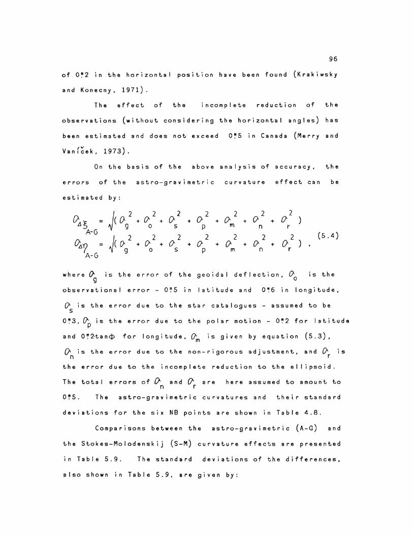
96

of 0~2 in the horizontal position have been found (Krakiwsky

and Konecny, 1971).

The effect of the incomplete reduction of the

observations (without considering the horizontal angles) has

been estimated and does not· exceed 0~5 in Canada (Merry and

fV ) Van1cek, 1973 .

On the basis of the above analysis of accuracy, the

errors of the astra-gravimetric curvature effect can be

estimated by:

{)..15 Jc o-g 2 2 o-2 + 0 2

2 2 2 = + ()' + + ()- + 0 + () )

0 5 p m n r A-G

2 2 2 2 2 02 (5.4)

~'? ~( (}g 2

) = + ()' + ()- + (} + (} + (} + 0 s p m n r

A-G

IS the w he r e o-9 i s the e r r or of the g eo i d a I de f I e c t i on , 00

observational error- 0~5 in latitude and 0~6 in longitude,

(}5 is the error due to the star catalogues- assumed to be

0 ~ 3 , l/-P i s t h e e r r o r d u e to t h e p o I a r mot i on - 0 ~ 2 f o r I a t i t u d e

a n d 0 ~ 2·t a n ¢ f o r I o n g i t u d e , (/-m i s g i v e n b y e q u a t i o n ( 5 . 3 ) ,

0 is the error due to the non-rigorous adjustment, and (} is n r

the error due to the incomplete reduction to the ellipsoid.

The total errors of () n

and 0' r

are here assumed to amount to

0!'5. The astra-gravimetric curvatures and their standard

deviations for the six NB points are shown in Table 4.8.

Comparisons between the astra-gravimetric (A-G) and

the Stokes-Molodenskij (S-M) curvature effects are presented

in Table 5.9. The standard deviations of the differences,

also shown 1n Table 5.9, are given by:

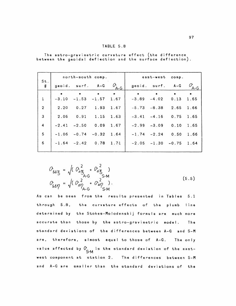
97

TABLE 5.8

The astra-gravimetric curvature effect (the difference between the geoidal deflection and the surface deflection).

north-south St.

# geoid. surf.

II II

1 -3.10 -1.53

2 2.20 0.27

3 2.06 0.91

4 -2.41 -2.50

5 -1.06 -0.74

6 -1.64 -2.42

comp.

A-G OA-G

II II

-1.57 1. 67

1.93 1. 67

1.15 1. 63

0.09 1.67

-0.32 1. 64

0.78 1. 7~

2 (}.15 )

S-M 2

{)'A'? ) .

S-M

east-west comp.

geoid. surf. A-G (} A-G

" II II II

-3.89 -4.02 0.13 1. 65

-5.73 -8.38 2.65 1. 66

-3.41 -4.16 0.75 1. 65

-2.99 -3.09 0.10 1. 65

-1.74 -2.24 0.50 1. 66

-2.05 -1.30 -0.75 1.64

(5.5)

As can be seen from the results presented in Tables 5.1

through 5.8, the curvature effects of the plumb I ine

determined by the Stokes-Molodenskij formula are much more

accurate than those by the astra-gravimetric model. The

standard deviations of the differences between A-G and S-M

are, therefore, almost equal to those of A-G. The only

value affected bv ~ is the standard deviation of the east-J S-M

west component at station 2. The differences between S-M

and A-G are smaller than the standard deviations of the

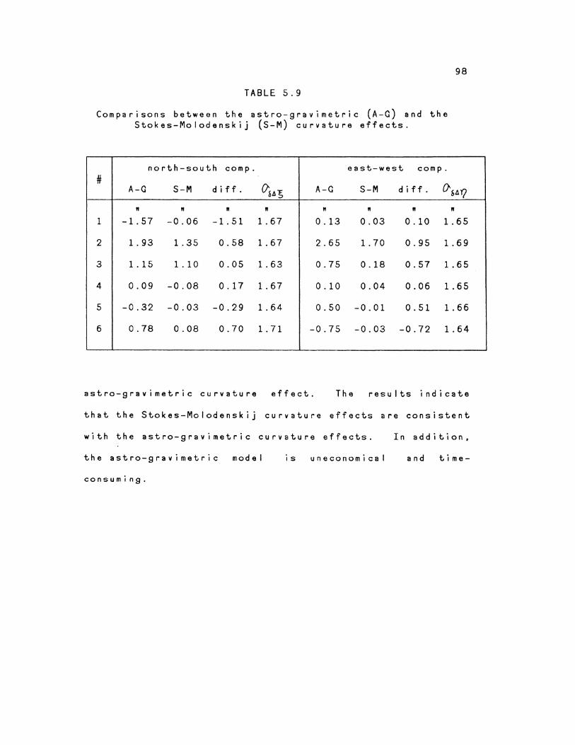
98

TABLE 5.9

Comparisons between the astra-gravimetric (A-G) and the Stokes-Molodenskij (S-M) curvature effects.

north-south comp. east-west comp. #

(/'~t\5 (}SA'Q A-G S-M d iff. A-G S-M diff.

" " " " " " " " 1 -1.57 -0.06 -1.51 1. 67 0. 13 0.03 0.10 1. 65

2 1. 93 1. 35 0.58 1. 67 2.65 1. 70 0.95 1. 69

3 1. 15 1. 10 0.05 1. 63 0.75 0.18 0.57 1. 65

4 0.09 -0.08 0.17 1. 67 0.10 0.04 0.06 1. 65

5 -0.32 -0.03 -0.29 1. 64 0.50 -0.01 0.51 1. 66

6 0.78 0.08 0.70 1. 71 -0.75 -0.03 -0.72 1. 64

astra-gravimetric curvature effect. The results indicate

that the Stokes-Molodenskij curvature effects are consistent

with the astra-gravimetric curvature effects. In addition,

the astra-gravimetric model ts uneconomical and time-

consuming.

CHAPTER 6

CONCLUSIONS AND RECOMMENDATIONS

Due to the uneven density distribution of the earth,

the plumb lines are bent and twisted. The curvature and

torsion are different from point to point and are very

localized. The effects are larger in mountainous areas than

in flat areas.

Some approaches for estimating the curvature effect

of the plumb line have been formulated and tested. If we

use the method based on the gravity field model, then the

density distribution has to be wei 1-known. If we use the

method based on the relation between the curvature effect

and the orthometric height correction, then a dense gravity

net around the computation point is needed.

accurate knowledge of the crustal densties

The need for

is self-evident

in using the method based on density model ling. Thus good

accuracies for the curvature effect of the plumb line from

those methods cannot be expected (Ndyetabula, 1974). If we

utilize Vening Meinesz's and Molodenskij 's formulae, i t

becomes laborious and time-consuming to calculate the

geoidal and Molodenskij's deflections separately in order to

determine the plumb line curvature effect.

- 99 -

100

The objectives of the work undertaken for this thesis

were to practically test another approach for the evaluation

of the plumb line curvature effect. The method, developed

by Van(~ek and Krakiwsky (1982). is based on the combination

of Stokes's and Molodenskij~s approaches. From the results

shown in the last chapter, the Stokes-Molodenskij curvature

effects are consistent with the astra-gravimetrically

determined curvature effects. but our method gives a much

hi'gher accuracy. In addition, it is easy to apply. The

determination of the curvature effect of the plumb line is

no Ion g e r a d iff i c u It work .

The analyses in Chapter 4 show that the contribution

of the difference between the free-air anomalies on the

geoid and those on the earth's surface is very small. It

can be neglected without loss of accuracy. The curvature of

the plumb line is mainly affected by the surrounding

topography to a spherical distance of < about 13

(approximately 24 km).

The Tables in last chapter demonstrate that the

terrain profile effects (point effects) along the north-

south and east-west directions are usually more significant

than the regional terrain and gravity effects. In other

words. the local terrain contributions dominate the

phenomenon. Therefore, the slopes of the terrain have to be

accounted for very carefully.

I

101

In this work, the method based on the combination of

Stokes's and Molodenskij's approaches is first tested to

determine the curvature effect of the plumb line. A formula

which combines the geoidal and Molodenskij's deflections of

the vertical is cal led the Stokes-Molodenskij formula. A

contribution is also made in the development of an algorithm

for numerical evaluation of the Stokes-Molodenskij formula.

Another contribution is made by formulating an algorithm for

terrain slope evaluation.

Since the curvature effect of the plumb line is

position-dependent and since the variation

point is large in mountainous areas, it is

from point to

difficult to

predict the plumb line curvature effect from the point plumb

Tables 5.1 through 5.6 show line curvatures already known.

that the contribution of the regional terrain and gravity

effect

smooth.

is at most about 0!1

For further studies,

in New Brunswick and seems

it is recommended that the

curvature effect of the plumb line may be computed for other

points in Canada. If the contributions of the regional

terrain and gravity effect are smooth, then it is also

recommended that the prediction of the plumb I ine curvature

effect may be done in two steps. First, use available data

for the contribution of the regional terrain and gravity

effect to predict the contribution of unknown point.

Secondly, determine from the topographic maps or field works

the local terrain contribution.

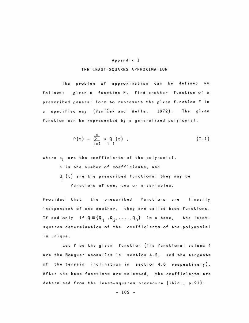
AppendiK I

THE LEAST-SQUARES APPROXIMATION

The problem of approKimation can be defined as

fol lows: given a function F' find another function of a

prescribed general form to represent the given function F In

a specified way ( , v Van1cek and We I Is, 1972). The given

function can be represented by a generalized polynomial:

n P(t) = L a·Q (t)

i=1

where a. are the coefficients of the polynomial, I

n is the number of coefficients, and

(I. 1)

Q. (t) are the prescribed functions: they may be I

functions of one, two or m variables.

Provided that the prescribed functions are linearly

independent of one another, they are called base functions.

If and only is a base, the I east-

squares determination of the coefficients of the polynomial

is unique.

Let f be the given function (The functional values f

are the Bouguer anomalies in section 4.2, and the tangents

of the terrain inclination 1n section 4.6 respectively).

After ~he base functions are selected, the coefficients are

determined from the least-squares procedure (ibid., p.21):

- 102 -

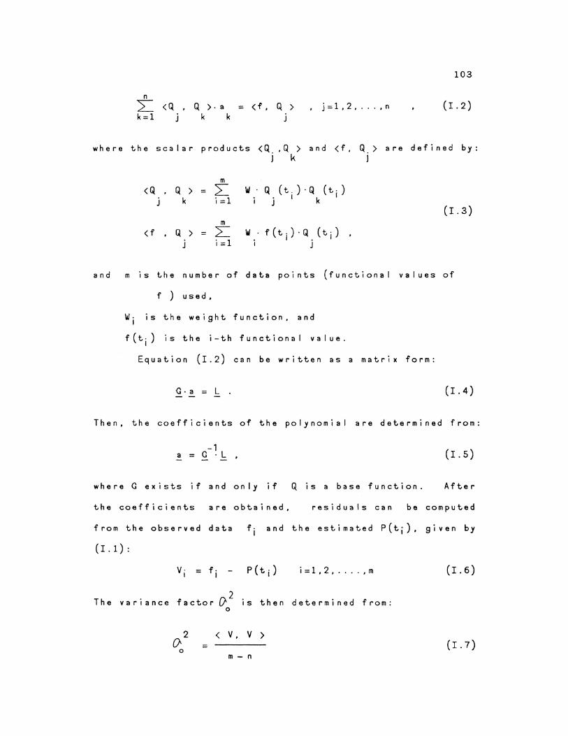
103

n

:L <Q, Q )-a = (f, Q > , j=1,2, ... ,n (I. 2) k=1 j k k

where the scalar products <Q .• Q >and (f, Q_> are defined by: J k J

m (Q ' Q > = ~ W· Q (t.)·Q (ti)

j k i=1 j I k (I. 3)

m <f ' Q > = 2:= w . f(ti)·Q. (tj)

j i=1 J

and m is the number of data points (functional values of

f ) used,

wi is the weight function, and

f(tj) is the i-th functional value.

Equation (I.2) can be written as a matrix form:

Q.a = L (I. 4)

Then, the coefficients of the polynomial are determined from:

-1 a = G · L (I. 5)

where G exists if and only if Q is a base function. After

the coefficients are obtained, residuals can be computed

from the observed data fj and the estimated P(tj). given by

(I.1):

The var1ance

i =1, 2, .... , m

() 2 factor is then determined from:

2 ()

0 =

0

< v' v >

m - n

(I. 6)

(I. 7)

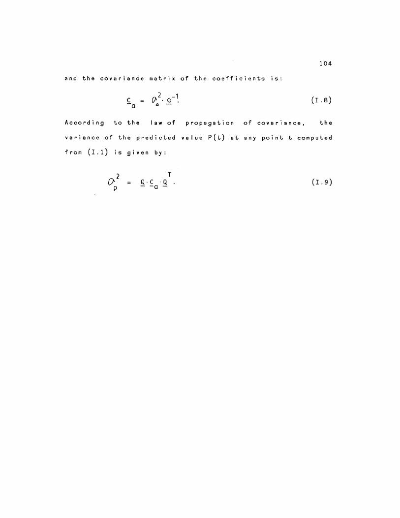
and the covariance matrix of the coefficients is:

According to the

().2 -1 v· · G •

0 -

law of propagation of covariance,

104

(I. 8)

the

variance of the predicted v·alue P(t) at any point t computed

from (I.l) is given by:

= T

Q. c . Q • - -a - (I. 9)

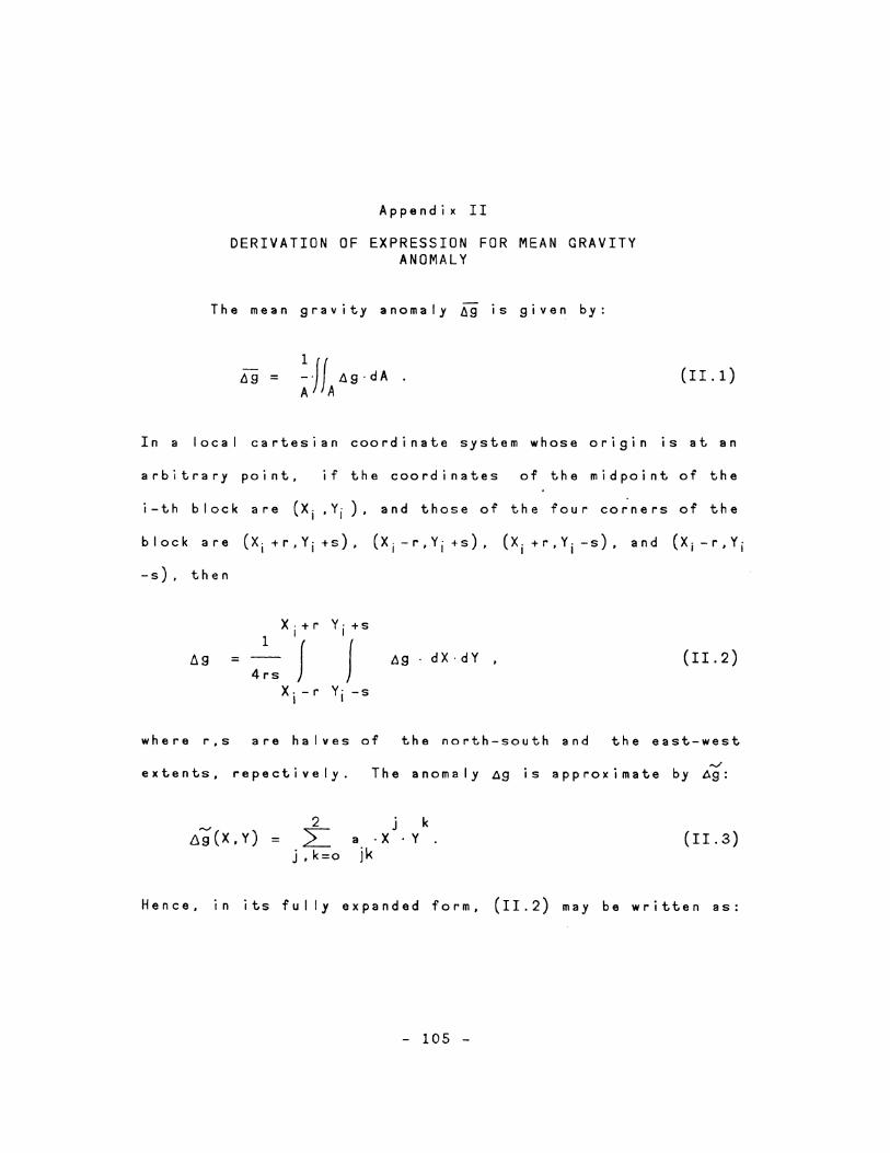
Appendix II

DERIVATION OF EXPRESSION FOR MEAN GRAVITY ANOMALY

The mean gravity anomaly ~g IS given by:

(II.l)

In a local cartesian coordinate system whose origin is at an

arbitrary point, if the coordinates of the midpoint of the

i-th block are (Xi ,Yj ), and those of the four corners of the

block are (Xi+r,Yj+s), (Xi-r,Yj+s), (Xi+r,Yi-s), and (Xi-r•Yi

-s), then

X-+r Y·+s

69 = 4 :5

'J 'J h9 · dX·dY , (II.2)

X--rY·-s I I

where r,s are halves of the north-south and the east-west

extents, repectively.

2 6g(X,Y) = L

j , k =o

..v The anomaly Ag is approximate by Ag:

j k a ·X · Y . jk

(II.3)

Hence, 1n its fully expanded form, (II.2) may be written as:

- 105 -

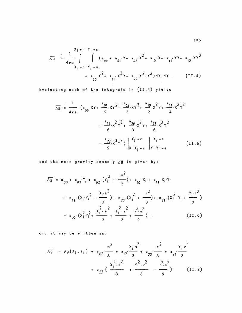
106

Yj+S

f ( 8 + 8 · Y + a · Y 2 + a · X+ a . X·Y + 8 · X·Y 2 00 01 02 10 11 12

X;-r Y;-s

2 + a . X +

20 (II.4)

Evaluating each of the integrals in (II.4) yields

1 .1g =

4rs

a12 2 3 a20 3 a21 3 2 + -·X y + -·X Y+ -·X y

6 3 6

.~1..2.x3 v3) I X H y. +S

I +

9 X=1Xi - r Y=Y; -s

(II.S)

and the mean gravity anomaly ll9 is given by:

2 52 llg = a 00 + a . y. + a .(v. + -)+ a ·X;+ a -X· ·Y;

01 ' 02 I 3 10 11 I

2 r2 y .. r 2 2 X;-s 2 2

+ a ·(X··Y· + - )+ a 20. (Xi + -)+ a 21 .(X; · Y; + -'-) 12 I I 3 3 3

2 2 2 2 X;· s

+ a 22 -(X;·Y; + + 3

or, it may be written as:

= llg ( X i • y i ) + a ·--02 3

2 2 Y; · r

3

2 r·s

+ 9

2 X-·s '

2

+ a .-- + 12 3

+ 3

)

2 r

a 20 3

2 2 r ·S

+ ) 9

(II.6)

2 y. ·r

I

3

(II.7)

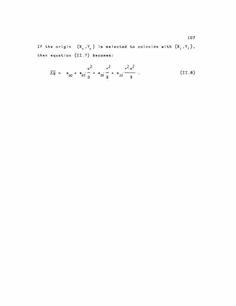
107

If the origin (X. ,Y.) is selected to coincide with (Xi ,Yi),

then equation (II.7) becomes:

2 2 r ·S

L':.g = a +a·-+ 00 02 3

a 20 3

+a·--22

(II.8) 9

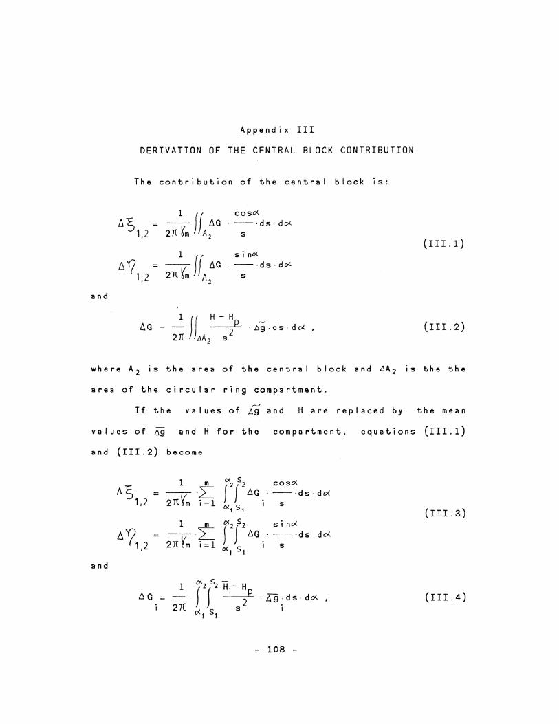
and

Appendix III

DERIVATION OF THE CENTRAL BLOCK CONTRIBUTION

The contribution of the central block

1 f! coso<. L1S = -- fiG · --·ds· do<. 1,2 2J1 ~m A2 s

sino<. -- ·ds. do(

s

is:

(III.1)

(III.2)

where A2 is the area of the central block and ~A 2 is the the

area of the circular ring compartment.

If the values of £9 and Hare replaced by the mean

values of 69 and H for the compartment, equations (III.1)

and (III.2) become

1 m =-·2:

2TC¥'m i =1

~ 52 coso< J { ~G.·-·ds·do< O(t 51 I S

o<2 5 2 sino( f J 6G.·-·ds-do<. 0( S I S

1 1

(III.3)

~ '?, 2 I

1 m

=-·2:: 2Jt~m i=1

and

o< s -A G -- _:_ . f 2f 2 Hi- H2p u ·Ag-ds-do<.,

21( o< 5 s f f

(III.4)

- 108 -

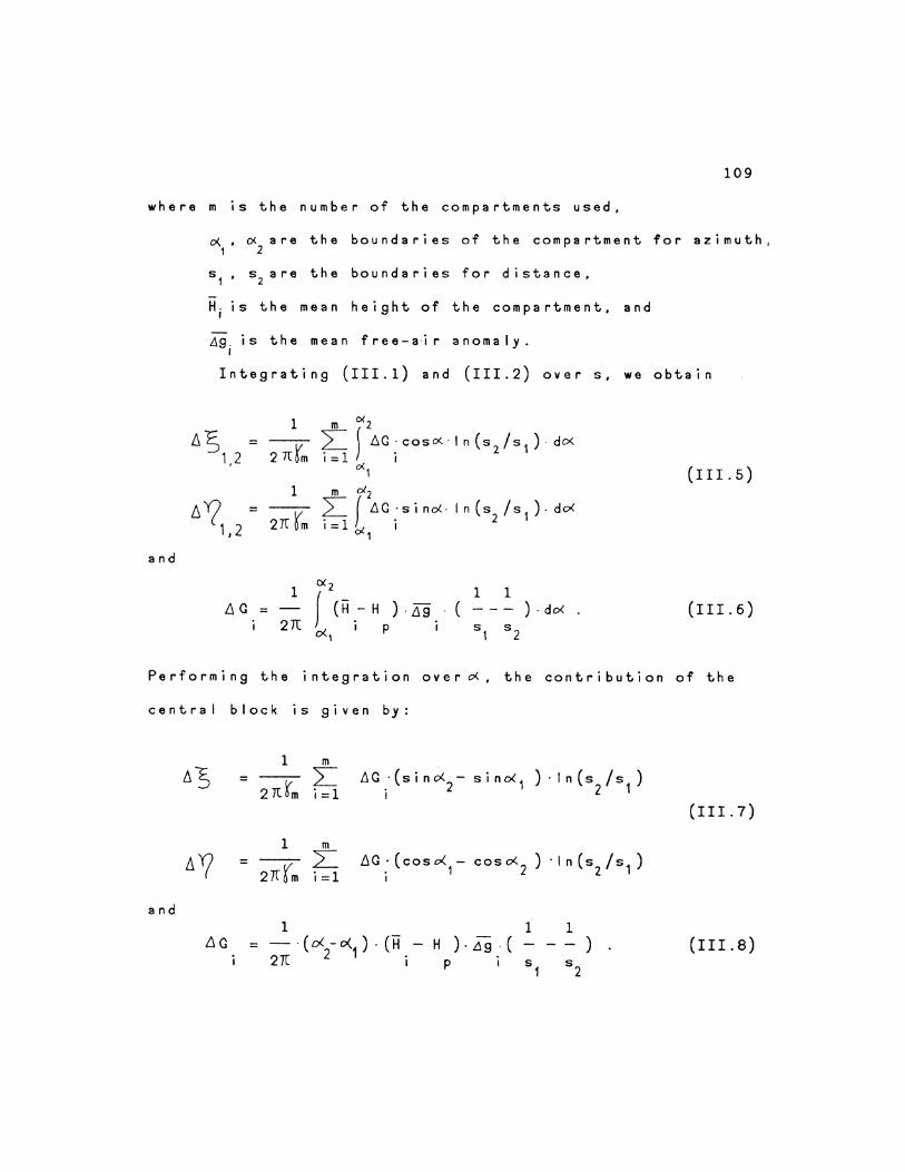
109

where m is the number of the compartments used,

~, ~ are the boundaries of the compartment for azimuth, 1 2

s 1 , s 2 are the boundaries for distance,

H; is the mean height of the compartment, and

..1g. is the mean free-a·ir anomaly. I

Integrating (111.1) and (111.2) overs, we obtain

1 m cx2

6 5,,2 = 2 1trm

?= J ~G:coso<.·ln(s 2 /s 1 )-do< 1=1 I

o(1 (111.5) 1 m d 2

{j 1,,2 = 27( rm

?=.{ .6G:sino(-ln(s2 /s 1 )-do< I= 1 Ol I

1

and

1 0(2

1 1 l\G = f (H.- H ) . ,6g .. ( ) . do<

27t o( I p I s, 52 1

(111.6)

Performing the integration over~. the contribution of the

central block is given by:

.6 G · ( s i n o<2 - s i no< 1 ) · I n ( s / s ) i 2 1

(III. 7)

.llG ·(coso< - coso<. 2 ) ·In (s /s 1 ) i 1 2

and 1 1 1

= - · ( o< - o<.1 ) · (H - H ) · .1g · ( 21( 2 . .

I p I s 1

) (III.8)

REFERENCES

Arnold, K. (1960). Numerische Beispiele zur strengen Theorie der Figur der Erde, Veroff. Inst. Postsdam, Neue Serie Nr.16, Germany.

Arnold, K. (1962a). Gravimetric Deflections of the Vertical i n H i g h M o u n t a i n s De t e r m i n e d by F r e e -A i r A nom a I i e s , ~!:!. 11 . Q~Q~ .• No. 63, pp. 73-74.

Arnold, K. (1962b). Recent Achievement in the Theory of the LeveiSurfaces of the Earth, ~!!.11· Q~Qg., No. 63, pp. 39-42.

Bomford, G. (1971). Q~QQ~§!y, Third Edition, Oxford University Press.

Derenyi, E.E. (1965). Q~f1~~tl2Gli! 2f th~ ~~rtl~~1 ln ~~ntr~1 ~~~ ~!!i.Q~~l~~. M.Sc.E. Thesis, Department of Surveying Engineering, University of New Brunswick.

Faucher, F. (1984). Personal Communication, Surveys and Mapping Branch, Geodetic Survey of Canada.

Graaff-Hunter, J.DE. and G. Bomford (1928). Q~Q~. B~f. ~!i.!Y· In~l~ ~. PP. 118-128.

Groten. E. (1981). Q~t~rmln!!.tl2n 2f th~ E1!!!!!Q l.:ln~ ~!!!Y!!.:!!!!!~ QY. ~~:!!!2!12!!!1~!!.1 !!.Qg Qr~Yl!!!~trl~ ~~th2~~. NOAA Tech n i c a I Memo r a n dum , N 0 S N G S -3 0 .

Gysen, H.V. (1980). Precise Gravimetric Deflections of the Vertical in the Canberra Area, ~!i.~"!!I!!.1l!!.n J. Q~Q~. Eh2:!!2· ~!!IY·· No. 32, pp. 1-43.

Heiskanen, W.A. and F.A. Vening Meinesz (1958). Ih~ ~!!.!"th !!. n ~ ! :t li! Q I !!. y l t Y. E l ~ 1 g , M c G r a w -H i I I 8 o o k C o . , I n c . , N e w York.

Heiskanen, W.A. and H. Moritz (1967). Ebt~l~!!.1 Q~QQ~~y. W.H. Freeman San Francisco.

Helmert, F.R. (1880). Ql~ ~~:th~!!!!!.:l!l~~h~n !!.!:!~ Ebtli!l~~ll~~h~n Ih~2rl~n ~~! tl2h~r~n Q~QQ~~l~. Vol. 2 Leipzig.

- 110 -

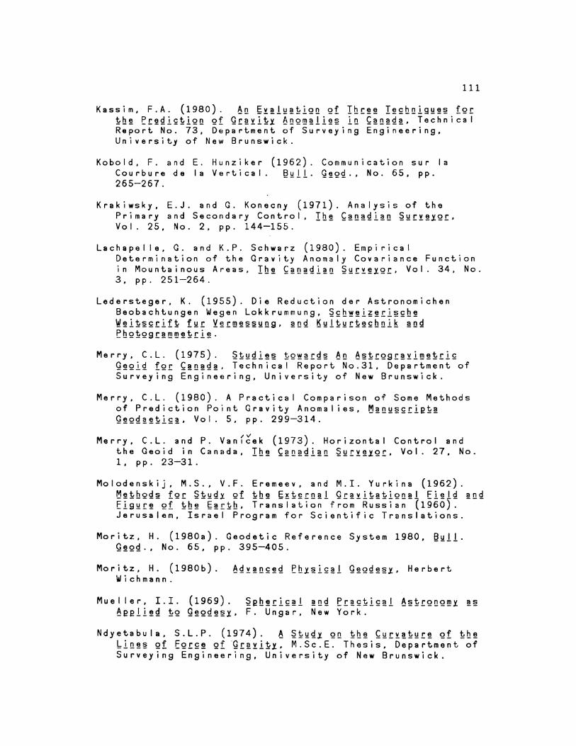
111

Kassim, F.A. (1980). An ~JU!!Y~!!lQn gf Ihr!!~ I!!ghnl9!U~ fgr !!h!! ~r~dlg!!lQn gf Qr~!l!!x AnQm~!l~~ ln ~~n~d~. Technical Report No. 73, Department of Surveying Engineering, University of New Brunswick.

Kobold, F. and E. Hunziker (1962). Communication sur Ia Courbure de Ia Vertical. ~!:!.!!. Q~QQ·, No. 65, pp. 265-267.

Krakiwsky, E.J. and G. Konecny (1971). Analysis of the Primary and Secondary Control, Ih! ~~n~dl~n ~l!.!:!~lQ.!:. Vol. 25, No. 2, pp. 144-155.

Lachapelle, G. and K.P. Schwarz (1980). Empirical Determination of the Gravity Anomaly Covariance Function in Mountainous Areas, Ih~ ~~n~dl~n ~l!.!:!~lQ!:. Vol. 34, No. 3 • p p . 2 5 1-2 6 4 .

Ledersteger, K. (1955). Die Reduction der Astronomichen Beobachtungen Wegen Lokkrummung, ~gh~~l~~rl~gh!!

W~l!!~grlf~ fYr ~!!m!~~yng. ~nd ~Y!~Yr~~ghnlk ~nd ~hQ~Qgr~mm~~rl!!·

Merry, C.L. (1975). ~~Ydl~~ tg~~rd~ An A!!~!:Q9!~!lm~trlg Q~glg fgr ~~n~d~. Technical Report No.31, Department of Surveying Engineering, University of New Brunswick.

Merry, C.L. (1980). A Practical Comparison of Some Methods of Prediction Point Gravity Anomalies, ~~nY!!grlet~ Q!!QQ~!~lg!. Vol. 5, pp. 299-314.

Merry, C.L. and P. Vanf~ek (1973). Horizontal Control and the Geoid in Canada, Ih~ ~~n~dl!n ~Y!!~lQ!, Vol. 27, No. 1 , p p . 2 3-31 .

Mo I ode n s k i j , M . S . , V . F . Ere me e v , and M . I . Y u r k i n a ( 19 6 2) . ~!~hQQ!! fgr ~~Ydx 2f ~h! E~~!!!l!l Qr!!l~!~lgn~! El!ld ~nd Elg!!.!!! gf ~h! ~!!~h. Translation from Russian (1960). Jerusalem, Israel Program for Scientific Translations.

Moritz, H. (1980a). Geodetic Reference System 1980, ~Yll· Q~QQ., No. 65, pp. 395-405.

Moritz, H. (1980b). Ad!!!lg!!d ~hx~lg~! Q!QQ!!!l· Herbert Wichmann.

Mueller, I.I. (1969). ~eh!!rlg~l !nd ~r~g~lg~! A~~!QnQml ~!! Aeell!!d !!Q Q!!QQ!!!!l• F. Ungar, New York.

Ndy.etabula, S.L.P. (1974). A ~tYdl Qn th~ ~Y!!~td!!!! gf !!h~ ~l!l!!!! Qf EQrg!! gf ·gr~!ltx. M.Sc.E. Thesis, Department of Surveying Engineering, University of New Brunswick.

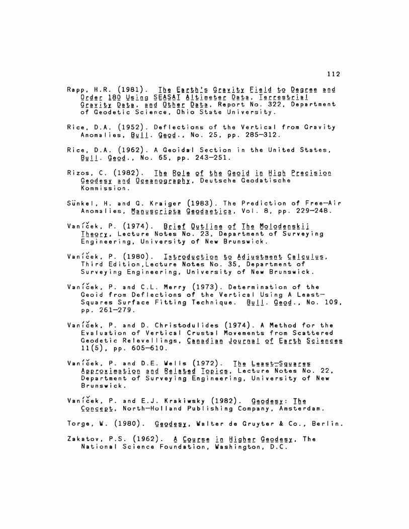
112

Rapp. H. R. (1981). !h!! !;!!1!h~~ g!!!1!!.x. E1!!1~ !!2 Q!!9!!!!! ~n9. Q.~:~!! !eQ ~~1ns ~~;~~~! ~11!1m!!1!!!! Q~1!!. I!!!r!!~1!.~:1!1 g!!!l1!.X. Q!!!!· !!lQ Q1!h!!! Q!!!!. Report No. 322, Department of Geodetic Science, Ohio State University.

Rice, D.A. (1952). Deflections of the Vertical from Gravity Anomalies, e~11. g!Q~ .• No. 25, pp. 285-312.

R i c e • D . A . ( 1 9 6 2 ) . A G eo i d a· I S e c t i o n i n t h e U n i t e d S t a t e s • ~~11. g!Q~ .• No. 65, pp. 243-251.

Rizos, C. (1982). !h!! B21!! 2f !!h!! Q!!Q1~ 1n t!1sh e!!21~12n Q!!Q~!!~.X. !!l~ Q2!!!!lQ9!!eh.x.. Deutsche Geodatische Kommission.

Sunkel. H. and G. Kraiger (1983). The Prediction of Free-Air An om a I i e s • ~! !l ~ ~ 2! 1 e!!! g!! Q g ~!! 1! 12! . Vo I . 8. p p . 2 2 9-2 48 .

Vanl~ek, P. (1974). e.~:1!!f Q~t11!l!! 2f !h!! ~2129.!n~!dl !h!!Q!Y• Lecture Notes No. 23, Department of Surveying Engineering, University of New Brunswick.

Vanf~ek, P. (1980). I~!!!Q~~2!!12!l 1!2 ~~l~~1!rn!!l!! ~!12~1~~. Third Edition,Lecture Notes No. 35, Department of Surveying Engineering, University of New Brunswick.

Vanf~ek, P. and C.L. Merry (1973). Determination of the Geoid from Deflections of the Vertical Using A Least­Squares Surface Fitting Technique. e~11. Q!Q9. .• No. 109, pp. 261-279.

Vanf~ek, P. and D. Christodulides (1974). A Method for the Evaluation of Vertical Crustal Movements from Scattered Geodetic ReI eve I I i ngs, ~!!!.~9.1!!!. 4Q~!!l!1 Qf E!!1!h ~21!!!!.2!!~ 11 (5). pp. 605-610.

V a n f ~ e k , P . a n d D . E . We I I s ( 19 7 2) . I b.! 6!!!!! :!!=-~ g ~!!!!!! ~ee!Q!1m~:l!12!!. !!!.Q B!!1!!!!~ !Qe12~. Lecture Notes No. 22. Department of Surveying Engineering, University of New Brunswick.

Vanf~ek, P. and E.J. Krakiwsky (1982). g!Q~h~y: !h!! ~Q!!.2!!e:l!. North-Hoi land Pub I ishing Company, Amsterdam.

Torge, W. (1980). Q!!Q!i!!~l· Walter de Gruyter & Co., Berlin.

Zakatov, P.S. (1962). ~ ~Q~!~!! 1!!. t!19h!H Q!Q~!!~Y· The National Science Foundation, Washington, D.C.