Evaluation of the performance of a pairs trading strategy

Evaluation of the performance of a

pairs trading strategy of JSE listed

firms

Shreelin Naicker

A research report submitted to the Faculty of Comme rce, Law and

Management, University of the Witwatersrand, in par tial fulfilment of the

requirements for the degree of Master of Finance an d investment.

Supervisor: Prof Eric Schaling

Johannesburg, 2015

ABSTRACT

A pairs trading strategy is a market neutral trading strategy that tries to

make a profit by making use of inefficiencies in financial markets. In the

equity pairs trading context, a market neutral strategy, is a strategy that

hedges against both market and sector risk. According to the efficient

market theory in its weak form, a pairs trading strategy should not

produce positive returns since the actual stock price is reflected in its past

trading data. The main objective of this paper is to examine the

performance and risk of an equity pairs trading strategy in an emerging

market context using daily, weekly and monthly prices on the

Johannesburg Securities Exchange over the period 1994 to 2014. A

bootstrap method is used determine whether returns from the strategy

can be attributed to skill rather than luck.

Key Words: pairs trading, quantitative strategy, asset allocation

DECLARATION

I, Shreelin Naicker, declare that this research report is my own work

except as indicated in the references and acknowledgements. It is

submitted in partial fulfilment of the requirements for the degree of Master

of Finance at the University of the Witwatersrand, Johannesburg. It has

not been submitted before for any degree or examination in this or any

other university.

-------------------------------------------------------------

Shreelin Naicker

Signed at ……………………………………………………

On the …………………………….. Day of ………………………… 2015

DEDICATION

To Presodhini, Adara, Callan and Custard

ACKNOWLEDGEMENTS

Thank you to my wife Prissy for her continual support, to my work

colleagues and class mates for their constant encouragement and to Prof

Eric Schalling.

TABLE OF CONTENTS

1. CHAPTER 1: INTRODUCTION ......................... ........... …….1

1.1 PURPOSE OF THE STUDY ............................................................................ 1

1.2 CONTEXT OF THE STUDY ............................................................................. 2

1.3 PROBLEM STATEMENT ................................................................................ 4

1.3.1 MAIN PROBLEM ...................................................................................................... 4

1.4 SIGNIFICANCE OF THE STUDY ...................................................................... 4

1.5 DELIMITATIONS OF THE STUDY..................................................................... 5

1.6 DEFINITION OF TERMS ................................................................................ 6

1.7 ASSUMPTIONS ........................................................................................... 8

2. CHAPTER 2: LITERATURE REVIEW ................. .............. 9

2.3. THE LAW OF ONE PRICE .............................................................................. 9

2.3. HISTORY OF PAIRS TRADING ........................................................................ 9

2.3. THE CAPM AND PAIRS TRADING .................................................................. 10

2.4. COMMONLY USED PAIRS TRADING METHODS ............................................... 15 2.4.1 THE DISTANCE METHOD ........................................................................................ 16 2.4.2 THE COINTEGRATION METHOD ............................................................................... 20

2.5. DOES A SIMPLE PAIRS TRADING STRATEGY STILL WORK ............................... 22

2.6. NEW DIRECTIONS IN PAIRS TRADING........................................................... 24

2.7. PRACTICAL ISSUES WHEN PAIRS TRADING ................................................... 25

3. CHAPTER 3: RESEARCH METHODOLOGY ................. ... 27

3.1 DATABASE ............................................................................................... 27

3.2 METHODOLOGY ....................................................................................... 27 3.2.1 PAIRS SELECTION ................................................................................................ 27 3.1.2 ASSESSING THE PERFORMANCE OF A PAIRS TRADING STRATEGY ............................. 29

3.3 BOOTSTRAP METHOD FOR ASSESSING PAIRS TRADING PERFORMANCE .......... 30

4. CHAPTER 4: PRESENTATION OF RESULTS .............. .... 33

4.1 RETURNS ANALYSIS ................................................................................. 33

4.2 RISK ANALYSIS......................................................................................... 36

4.3 SKILL VS. LUCK ....................................................................................... 38

5. CHAPTER 5: CONCLUSIONS AND RECOMMENDATIONS …………………………………………………………………….41

REFERENCES .............................................................................. 42

APPENDIX A ........................................ ......................................... 47

TABLE 5: LIST OF SHARE CODES USED .................................................................. 47

LIST OF FIGURES

Figure 1: An example of Pairs Trading.…………………………………… ..3

Figure 2: CAPM and pairstrading…………………………………………...15

Figure 3: Anglo Gold and Gold Fields closing price data ………………17

Figure 4: Normalized Anglo Gold closing price……………………………17

Figure 5: Normalized Gold Fields closing price……………………………17

Figure 6: Difference between normalised AngloGold and GoldFields share price…………………..…………………………………………………19

Figure 7: Threshold vs Number of Trades………………………………….34

LIST OF TABLES

Table 1: Pairs Trading Raw Returns………………………………………..33 Table 2: Pairs Trading Long and Short Positions………………………… 35 Table 3: Pairs Trading Jensen's Alpha and Beta………………………….36 Table 4: Pairs Trading Returns versus Bootstrap……………………...….40 Table 5: List of share codes used ……………….……………………...….47

1

1. CHAPTER 1: INTRODUCTION

1.1 Purpose of the study

This paper aims to investigate the profitability of a pairs trading strategy

on the Johannesburg Securities Exchange using the distance approach.

It builds on similar studies done by Perlin (2006).

This study will aim to prove whether or not a pairs trading strategy is

profitable by using a model designed in MATLAB and based on

information gained from literature and financial market practitioners.

The Johannesburg Securities Exchange (JSE) is the 16th largest in the

world, and by far the largest of Africa's 22 stock exchanges. Market

capitalisation of the JSE at the end of December 2003 stood at R4 029-

billion, up from R1 160-billion five years earlier. In 2003 the JSE had an

estimated 472 listed companies and a market capitalisation of

US$182.6 billion (€158 billion), as well as an average monthly traded

value of US$6.399 billion (€5.5 billion). As of 31 December 2012, the

market capitalisation of the JSE was at US$903 billion. However, it is

much less liquid than that found in the United States and parts of

Europe and Asia.

There are many studies on pairs trading strategies in the United States

and Europe but very few have been done in the emerging markets

context and even fewer done in stressed markets. Financial market

stress occurs when there is a loss of liquidity, risk aversion, increased

volatility and falling valuations in emerging as was as developed

economies. As a result financial institutions find it difficult to secure

funding to finance their short term liabilities.

2

Since a pairs trading strategy requires implementing two trades instead

of one, evaluating performance in a less liquid market provides

additional evidence regarding the strategy's global implementable

efficacy. Pairs trading or statistical arbitrage as it is sometimes called, is

based on the law of one price, but is not riskless as the word arbitrage

suggests. There is embedded risk in the strategy which stems from

different economic fundamentals like market liquidity.

1.2 Context of the study

Pairs trading is often referred to as a trading strategy that is market

neutral, which attempts to identify financial instruments with similar

characteristics. In order for pairs trading to be effective as a trading

strategy the characteristics of these shares needs to be consistent over

a period of time. A pairs trading strategy is easy to implement and has

become very popular with traders throughout the world. Where a trader

or fund manager finds two stocks whose prices move together over a

window of time, the pairs trading strategy may be implemented when

price relationship of the instruments differs from that obtained in their

historical trading range, i.e. the two instruments prices are no longer

consistent anymore. The undervalued instrument is bought, and an

equally large short position is simultaneously instigated in the

overvalued instrument. Pairs trading is based on the fact that long term

historical price relationships outweigh short term price deviations over

time which results in a trader making profit. Pairs trading has been used

successfully by hedge funds and proprietary trading desks for many

years. However, the pairs trading strategy or arbitrage trading as it is

sometimes called, is not completely riskless. Once a trader has entered

into a pairs trade, the trader will ultimately lose money should the gap

3

between the two financial instruments widen, while the trader holds the

position. Therefore, any trader would want to enter a pairs trade when

the price gap between the trades is at its widest, and close his positions

when the price gap between the two instruments is at its widest in the

opposite direction. Pair trades are near market neutral and are based

on relative valuation which can easily be automated. Pairs trading has

become a popular investment strategy amongst investors as it promises

to give substantial profits irrespective of market conditions. A pairs

trading strategy removes systematic risk from portfolios and the investor

is only subjected to asset specific risk. Pairs trading involve essentially

constructing a portfolio of matching stocks in terms of systematic risks

but with a long position in the stock perceived to be under-priced and a

short position in the stock perceived to be overpriced. This would

result in a portfolio where systematic risk is hedged.

Figure 1: An example of pairs trading

The largest gap between the 2 shares prices is indicated by the blue

and red arrows, showing the entry and exit points of the trade. In order

for a trader to earn a maximum profit, a trade will be instigated at the

blue arrow, where a trader would short sell the green share and at the

4

same time go long the pink share. The trader will exit the share at the

red arrow but will make a profit on both the long and the short postion.

1.3 Problem statement

1.3.1 Main problem

Analyse the profitability and risk of a hedge fund trading strategy based

on the distance approach to pairs trading. While pairs trading is a

popular trading strategy used by hedge funds, it is not exclusively a

hedge fund strategy and can be used across any asset class to hedge

market risk. This analysis will cover daily, weekly and monthly

frequencies for stocks traded on the JSE across different distance

values. This research project extends the work of a number of

researchers such as Gatev et al (1999) and Perlin (2006), who have

conducted similar research in other markets. Many of the studies on

Pairs Trading have been conducted on exchanges that are far more

liquid than the JSE.

1.4 Significance of the study

Whereas there have been studies on pairs trading in the South African

agricultural market and Pairs trading on the single stock futures market

on the JSE, this research project aims to fill a gap in research by

analysing a pairs trading strategy using the distance approach on single

stock shares traded on the JSE. This research project will help

researchers and practitioners obtain a better understanding of such a

5

strategy in the context of an emerging market as well as gain an

understanding of how the market has changed from 1994 to 2014.

1.5 Delimitations of the study

• Trading costs were estimated and based on the current trading

costs on the JSE.

• Daily closing prices were used for all trading simulations. There is

sometimes a difference between closing prices and trading prices

6

1.6 Definition of terms

Long Position: The buying of a security such as a stock, commodity or

currency, with the expectation that the asset will rise in value.

Short Position: The sale of a borrowed security, commodity or

currency with the expectation that the asset will fall in value.

Liquidity: The degree to which an asset or security can be bought or

sold in the market without affecting the asset's price. Liquidity is

characterized by a high level of trading activity. Assets that can be

easily bought or sold are known as liquid assets.

S&P 500 Index: An index of 500 stocks chosen for market size, liquidity

and industry grouping, among other factors. The S&P 500 is designed

to be a leading indicator of U.S. equities and is meant to reflect the

risk/return characteristics of the large cap universe. Companies

included in the index are selected by the S&P Index Committee, a team

of analysts and economists at Standard & Poor's. The S&P 500 is a

market value weighted index in which - each stock's weight is

proportionate to its market value.

Hedge fund: A hedge fund is a collective investment scheme, often

structured as a limited partnership that invests private capital

speculatively to maximize capital appreciation. Hedge funds tend to

invest in a diverse range of markets, investment instruments, and

strategies; today the term "hedge fund" refers more to the structure of

the investment vehicle than the investment techniques. Though they are

privately owned and operated, hedge funds are subject to the regulatory

restrictions of their respective countries.

7

Market Neutral Strategy: A market neutral strategy is a strategy that

hedges against both market and sector risk, i.e., the expected return

from the strategy is uncorrelated with the market.

JSE: The Johannesburg Securities Exchange (JSE) is the 16th largest

in the world, and by far the largest of Africa's 22 stock exchanges.

Market capitalisation at the end of December 2003 stood at R4 029-

billion, up from R1 160-billion five years earlier. In 2003 the JSE had an

estimated 472 listed companies and a market capitalisation of

US$182.6 billion (€158 billion), as well as an average monthly traded

value of US$6.399 billion (€5.5 billion). As of 31 December 2012, the

market capitalisation of the JSE was at US$903 billion.

MATLAB: MATLAB (matrix laboratory) is a numerical computing

environment and fourth-generation programming language. Developed

by MathWorks, MATLAB allows matrix manipulations, plotting of

functions and data, implementation of algorithms, creation of user

interfaces, and interfacing with programs written in other languages,

including C, C++, Java, and FORTRAN.

Bloomberg: The Bloomberg Terminal is a computer system provided

by Bloomberg L.P. that enables professionals in finance and other

industries to access the Bloomberg Professional service, through which

users can monitor and analyse real-time financial market data and place

trades on the electronic trading platform. The system also provides

news, price quotes, and messaging across its proprietary secure

network.

8

1.7 Assumptions

• It is assumed that the daily closing prices available from Bloomberg

are accurate. The data was obtained using the historical data tool

provided in excel. Data was analysed for improbable shocks and

shares with improbable time series data were removed.

• Liquidity – it is assumed that there is a willing buyer and willing seller

at any time, so that liquidity is guaranteed any time in the model.

The pairs trading model designed in MATLAB relied heavily on this

assumption. It is important to note that this model does not try to

compensate for a lack of liquidity in the market.

• Trading costs - are constant over time – An analysis of JSE

historical trading costs shows that the costs varied across the time

period considered for this model. This model does not take into

account variable trading costs across time but uses a constant 1% of

the investment as trading costs. According to the latest cost tables

provided by the JSE this is a reasonable assumption.

• It was assumed that capital for short positions was not required. This

is consistent with research done by other researchers on this topic

and is realistic in terms real market conditions. To accomplish short

selling, you borrow shares of stock and then sell them in the open

market, without ever owning the shares. Then you must buy identical

shares back at a later date to return to the owner, your goal as a

short seller is to purchase the shares back for less cost in the future

and net a profit.

9

2. CHAPTER 2: LITERATURE REVIEW

2.1 The Law of One Price

The law of one price states that that if the returns from two investments

are identical in every state then the current value of the two investments

must be the same (Ingersoll 1987). Similarly, for markets to be perfectly

integrated (which is commonly assumed), two portfolios created from

two markets cannot exist with different prices if the pay offs are identical

(Chen and Knez 1995). If these conditions are not satisfied, arbitrage

opportunities exist thus giving investors opportunities to make risk-free

profits by buying under-priced securities and short-selling the overpriced

ones (Lamont and Thaler 2003). In a perfectly efficient market, the

prices fully react to the available information at all times (Fama 1970).

The market efficiency hypothesis reached its peak in 1970's, and at that

time there was a consensus on the idea that as soon as any news

reached the market it spreads quickly and immediately gets reacted to

through stock prices changes.

2.2 History of Pairs Trading.

The increase in processing powers of computers led to more

sophisticated trading models being developed and employed in

investment banks. Teams were formed to use statistical methods, to

develop computer based algorithms, which contained specific trading

rules and where human subjectivity had no influence whatsoever in the

process of trading. Many of these algorithms were successful for short

periods of time but did not show great consistency. Nunzio Tartalia, a

quant in Wall Street, assembled a team of mathematicians, physicists

10

and computer scientists in the mid 1980’s to design these algorithms to

be used for trading the equity markets. This group of former academics

used sophisticated statistical methods to develop high-tech trading

programs. These programs used trading rules to replace the intellectual

skill of traders with years of trading experience. A popular and

successful trading rule or strategy that emerged was a program that

identified pairs of securities whose prices tended to move together. It

was reported that this group made a $50 million profit for the Morgan

Stanley group based on the pairs trading strategy. Although the team

had a few years of bad performance, the pairs trading strategy gained a

good reputation in the financial markets and has since become an

increasingly popular "market-neutral" investment strategy used by

individuals and institutional traders as well as hedge funds. Pairs trading

is now used across many asset classes and is used widely in both

vanilla and derivative markets.

2.3 The CAPM and Pairs Trading

The CAPM model, essentially divides total risk, into two components

namely systematic risk, which is the risk associated with holding a

market portfolio, and asset specific risk which is the risk associated with

the specific asset. The objective of a market neutral strategy is to

remove systematic risk from a portfolio. According to the CAPM model

the portfolio would then only be subjected to asset-specific risk. One of

the market neutral strategies used to achieve this is to buy the

undervalued asset and short selling the overvalued asset. When market

forces affect the long asset, it is offset by the short position which

results in an elimination of systematic risk. This is the basis of a pairs

11

trading strategy which is a market neutral strategy as it involves taking a

long and short position on relatively mispriced assets.

According to Vidyamurthy (2004) CAPM is an acronym for capital asset

pricing model a formalisation of the notion of a market portfolio. A

portfolio of assets that acts as a proxy for the market can be thought of

as a market portfolio in CAPM terms. By using the ideas of beta and

market portfolio, the CAPM model, attempts to explain asset returns as

an aggregate sum of component returns.

The return on an asset can be broken up into two parts, the systematic

component (sometimes referred to as the market component) and the

non-systematic component. If

r� is the return on the asset,

r� is the return on the market portfolio,

beta of the asset is denoted as β,

then the formula showing the relationship that achieves the separation

of the returns is given as

r� = βr� + θ�

, which is also often referred to as the security market line (SML).

βr� is the market or systematic component of the return. β serves as a

leverage number of the asset return over the market return. It may also

be deduced from Figure 2 that β is indeed the slope of the SML. θ� in

the CAPM equation is the residual component or residual return on the

12

portfolio. It is the portion of the asset return that is not explained by the

market return. The consensus expectation on the residual component is

assumed to be zero.

If one was to separate the asset returns into its two components as

described by the CAPM model, the model elaborates on a key

assumption with respect to the relationship between them. This

assertion of the CAPM model is that the market component and residual

component are uncorrelated.

It was deduced earlier, that beta is the slope of the SML. By using the

returns from the market and the returns from the asset, beta can be

estimated as the slope of the regression line between the two. When

the standard regression formula is applied to estimate the slope, one

can conclude that the beta is the covariance between the asset and

market returns divided by the variance in market returns.

β = cov(r�r�)var(r�)

A positive return for the market usually implies a positive return for the

asset.

This implies that the sum of the market component and the residual

component would then be positive. One can then deduce that if the

residual component of the asset return is small then the positive return

in the asset would be explained almost completely by its market

component. A positive return in the market portfolio and the asset would

imply a positive market component of the return. Thus beta would have

a positive value. All assets would therefore be expected to have positive

values for their betas.

13

A market neutral strategy is a strategy that hedges against both market

and sector risk i.e. the return from the strategy is uncorrelated with the

market. Thus the market neutral strategy does not concern itself with

the state of the market (i.e. whether the market is going up or coming

down) but rather, it is more focussed on producing profits in a steady

manner, regardless of volatility.

We therefore would need a market neutral portfolio to trade? According

to the CAPM model, a market neutral portfolio would have zero beta. By

applying a zero value to the beta of the SML equation, one would find

that the return on the portfolio would not have a market component and

would completely be determined by θp which is the residual component

of the equation. The component of the model that remains is

uncorrelated with market returns, so that neutral returns are obtained

and thus the criteria met of a market neutral strategy due to a zero beta.

Since the mean of the residual return is zero, a strong mean reverting

behaviour can be expected, of the residual time series. Unexpected

market events and market forces that result in changes in supply and

demand usually result in changes in asset prices away from their

equilibrium price. Mean reversion can be described as the process of

asset prices moving away from their normal levels and then reverting

back. The exploitation in the process of return prediction of this mean

reverting behaviour can lead to trading signals which can then be used

to develop a trading strategy.

Using the definition of a market neutral strategy portfolio, we can

construct a portfolio with a zero beta. A portfolio that only has long

positions will have a positive beta and a portfolio with only short

positions will have a negative beta. A negative beta means that an

asset returns tends to move in the opposite direction to the markets

14

returns i.e. there is a negative correlation between the assets returns

and the market, and a positive beta means that the assets returns tend

to move in the same direction as the markets returns i.e. there is a

positive correlation between the assets returns and the market.

Therefore in order to construct a zero beta portfolio we cannot only use

assets that have positive betas or assets that only have negative betas

because this would not be possible. The only possibility would be to

hold both long and short positions on different assets in a portfolio. Due

to the fact that a zero beta portfolio has to comprise of both long and

short positions these portfolios are often referred to as long-short

portfolios.

Pairs trading is a market neutral portfolio that consists of just two

securities and is a market neutral strategy in its most primitive form,

which has one security as a long position and the other a short position.

The spread of an asset is the difference between the bid and offer of a

security or asset. The bid price is the maximum price that a buyer is

willing to pay for a security and the offer price is the minimum a seller is

willing to receive for a security. The spread is computed using the

quoted prices of the securities. A portfolio is associated with the spread

at any given time. In the CAPM equation the spread is related to the

residual return component of the return. The spread represents the

degree of mispricing of an asset or security and the higher the spread,

the higher the mispricing and the greater the chance to capture a profit.

A pairs trade would be executed when the spread is substantially wide

with the expectation that the spread will revert back to its mean. When

this convergence occurs the positions would then be reversed and a

profit would be made. Pairs Trading is based on the fact that in relative

15

pricing, stocks with similar characteristics would be priced relatively the

same.

Figure 2: CAPM and Pairs Trading

Source: Pairs Trading: Quantitative Methods and Analysis

2.4 Commonly used Pairs Trading methods

Nunzio Tatalia was a quantitative analyst who worked for Morgan Stanley in

the 1980’s and pioneered the pairs trading method. Since, the Nunzio

Tartalia days of pairs trading many quantitative analysts and financial

market practitioners have tried to replicate his team’s work to come up

with better methodologies in order to do achieve better results. The two

main commonly used methods in pairs trading are called the distance

method and the co-integration method, and recently the stochastic

spread method has become popular. The distance method is used in

Gatev et al (1999) and Nath (2003) for empirical testing whereas the

cointegration method is detailed in Vidyamurthy (2004). Both of these

are known to be widely adopted by practitioners. The stochastic spread

approach was recently proposed in Elliot et al (2005).

16

2.4.1 The Distance Method

The distance method is used in Gatev et al (1999) and Nath (2003) for

empirical testing. Under the distance method, the co-movement of a

pair is measured by what is known as the distance, or the sum of

squared differences between the two normalized price series.

D =��

��(P�� + P��)�

P��,P�� = normalised asset price.

The normalisation of prices for each security is done by subtracting the

sample mean of the training period, and dividing by the sample

standard deviation over the training period. A record is kept of the

distribution of distances between each pair over the training period. One

cannot use the original prices when using the minimum squared

distance due to the fact that two securities can move together, but the

squared distance between them could still be high. Therefore the

normalization of prices is the technique to use in order to prevent this.

After the normalization, stocks will be brought to the same standard unit

and allows for a quantitatively fair formation of pairs.

In order to normalize the price data, the mean and standard deviation

need to be calculated. A trade trigger can then be created by using the

difference between the normalized prices, which is illustrated by the

transformation below. A trade trigger is a market condition that results in

an automated execution of a trade (either buying or selling).

17

P��∗ =P�� − E(P��)

σ�

Where,

P��∗ = Normalised price of asset i at time t

E(P��) = Expectation of P�� (in this case the average)

σ� = Standard deviation of respective stock price

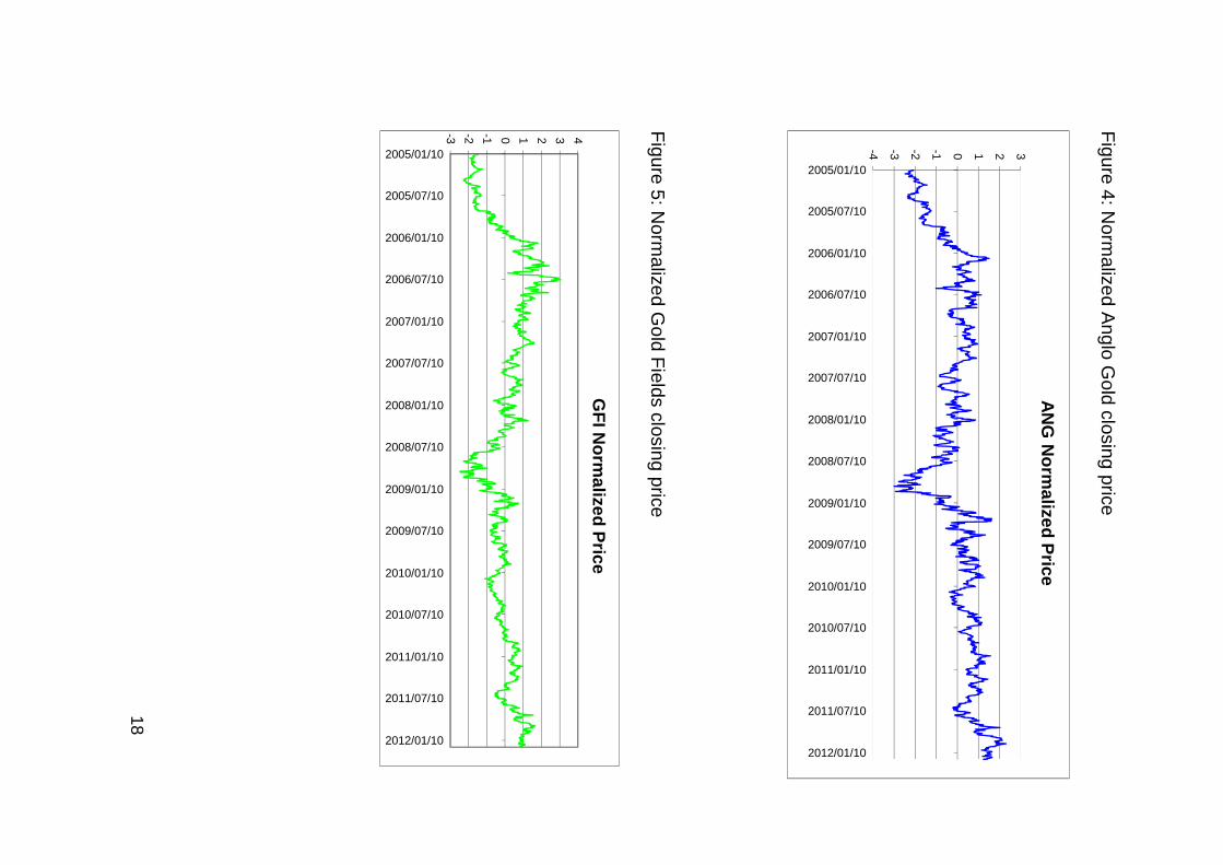
This is demonstrated below using the Anglo Gold and Goldfields daily

closing prices, which are shares, traded on the JSE.

Figure 3: Anglo Gold and Gold Fields closing price data

05000

1000015000200002500030000350004000045000

2005

/01/

10

2005

/07/

10

2006

/01/

10

2006

/07/

10

2007

/01/

10

2007

/07/

10

2008

/01/

10

2008

/07/

10

2009

/01/

10

2009

/07/

10

2010

/01/

10

2010

/07/

10

2011

/01/

10

2011

/07/

10

2012

/01/

10

Pric

e

ANG GFI Close Daily Price

18

Figure 4: N

ormalized A

nglo Gold closing price

Figure 5: N

ormalized G

old Fields closing price

-4 -3 -2 -1 0 1 2 3

2005/01/10

2005/07/10

2006/01/10

2006/07/10

2007/01/10

2007/07/10

2008/01/10

2008/07/10

2009/01/10

2009/07/10

2010/01/10

2010/07/10

2011/01/10

2011/07/10

2012/01/10

AN

G N

ormalized P

rice

-3 -2 -1 0 1 2 3 4

2005/01/10

2005/07/10

2006/01/10

2006/07/10

2007/01/10

2007/07/10

2008/01/10

2008/07/10

2009/01/10

2009/07/10

2010/01/10

2010/07/10

2011/01/10

2011/07/10

2012/01/10

GF

I Norm

alized Price

19

Figure 6: Difference between normalised Anglo Gold and Gold Fields

share price.

One can trade by using the mean reverting bias demonstrated above. In

normal daily trading activity, changes in supply and demand and

unexpected news events can result in asset prices moving away from

their equilibrium price. The process of asset prices moving away from

the equilibrium price and reverting back again is a demonstration of

what is known as a mean reversion process.

Another common practice amongst practitioners is to use the

normalized difference between prices, sometimes referred to as the

spread between market prices. In this approach, the equation above is

still used, but with P�� replaced by d�� the difference between prices.

d��∗ =d�� − E(d��)

σ�

Where d��∗ = P�� – P��

-2.5

-2

-1.5

-1

-0.5

0

0.5

1

1.5

2

2005

/01/

10

2005

/05/

10

2005

/09/

10

2006

/01/

10

2006

/05/

10

2006

/09/

10

2007

/01/

10

2007

/05/

10

2007

/09/

10

2008

/01/

10

2008

/05/

10

2008

/09/

10

2009

/01/

10

2009

/05/

10

2009

/09/

10

2010

/01/

10

2010

/05/

10

2010

/09/

10

2011

/01/

10

2011

/05/

10

2011

/09/

10

2012

/01/

10

Difference between normalised ANG and GFI prices

20

Trading rules can be set up once more information about the spread

and price behaviour is available. When a distance is above or below a

threshold trading can commence. The threshold controls when a

divergence is not considered normal i.e. as the threshold grows, fewer

and fewer abnormal divergences are found, which results in the

reduction in the number of transactions made by the strategy. This does

not depend on transaction costs.

2.4.2 The Co-Integration method

The co-integration method is more complicated than the distance

method and requires statistical analysis to implement through a pairs

trading strategy. According to Vidyamurthy (2004) the co-integration

method attempts to parametrize pairs trading strategies exploring the

possibility of co-integration. Order of integration is a summary statistic

for a time series that reports the minimum number of differences

required to obtain a covariance stationary series and is denoted by �( ) where represents the order. In statistics co-integration is a property

where two time series that are integrated of order 1 denoted by �(1) can

be linearly combined to produce a single time series which is order 0, or

�(0), and is stationary. According to Caldeira and Moura (2013), in

general, linear combination of non-stationary time series are also non-

stationary, thus not all possible pairs of stocks co-integrate.

A (# × 1) time series vector %& is co-integrated if each of its elements

individually are non-stationary and there exists a nonzero vector 'such

that '%& is stationary.

21

Pairs trading involves investing equal amounts in asset ( and asset),

which is achieved by short selling asset ) and investing the amount in *

shares of asset ( where *+&, = *+&- represents a cashless investment.

The idea of pairs trading is to invest an equal amount in asset ( and

asset),*+&, = *+&-, making this a cashless investment.

Thus by taking the log of the equation:

0 = log(*) + log(+&,) − log(+&-) (1)

The minus sign reflects the fact that asset ) is sold short. The log-return

on this investment over a small horizon (0 − 1, 0) is given by

log 2 34534675 8 − log 2 349

34679 8(2)

In order to make a profit the investor would not need to predict the

behaviour of +&, and +&- but only the difference

log(+&,) − log(+&-)

If we assume that :log(+&,) , log(+&-); in equation (1) is a non-stationary

<(=(+)process, and there exists a value > such that log(+&,) − >log(+&-) is stationary by our definition we have a co-integrated pair.

The investment equation will then become

22

0 = log(*) + log(+&,) − > log(+&-)(3)

The value of > will be determined by the co-integration, and the long run

equilibrium relationship between the assets determines *. The return on

the investment will be

log 2 34534675 8 − >log2 349

34679 8 (4)

If > = 1, the investor is able to profit from the trade, even though the

investment has an initial value of 0. A > close to zero requires funds to

invest in A. A large > exposes the investor to risk of going short on ).

2.5 Does a simple Pairs Trading strategy still work?

According to Binh Do et al (2009) a simple pairs trading strategy (equity

convergence trading strategy) was found to be profitable over a long

period of time although at a declining rate. The study showed that the

mean return for the period 1989- 2002 was 60% less than the mean

return for the period 1962-1988. By extending the work of Gatev et al

(1999), Binh Do et al (2009) found no evidence to suggest that the

profitability decline was due to increased competition in the hedge fund

industry. The main reason for the decline was found to be a decreasing

number of shares that did not converge within the trading period. This

was attributed to a break down in the Law of One Price upon which this

trading strategy is based. It is a requirement of the Law of One Price

23

that two assets that are close economic substitutes in the training period

continue to be so in the trading period.

It was also found that there was an increasing probability that close

economic substitutes defined in the historical price space did not remain

close substitutes in the trading period. The assertion was made that the

increased fundamental risk was the reason that industry practitioners

shied away from this strategy.

It was suggested in Binh Do et al (2009) that one should form pairs of

fundamental similarity which not only avoids unnecessary costs but

would also reduce non-convergence risks. In practice trading algorithms

should contain risk mitigating tools like stop loss which will minimize the

impact of divergent trades. One of the drawbacks of the simple pairs

trading strategy is that a pair may have a high historical spread but is

still used a recognised pair due to the fact that it has one of the lowest

spreads for the training period i.e. the pair are close economic

substitutes in the training period but in the trading period the pair have a

higher spread. It was suggested that a superior method would be to

form pairs based on a number of criteria and the best strategy

sometimes is to do nothing.

It was found in Binh Do et al (2009) that periods of high market volatility

could result in divergence being driven further. The divergence rate was

regressed against the market volatility proxied by the relevant six month

return standard deviation of the S&P 500 index1 . Thus a positive

1 The S&P 500, or the Standard & Poor's 500, is a stock market index based on the market capitalizations of 500 leading companies publicly traded in the U.S. stock market, as determined by Standard & Poor's. It differs from other U.S. stock market indices such as the Dow Jones Industrial Average and the Nasdaq due to its diverse constituency and weighting methodology. It is one of the most commonly followed equity indices and many consider it the best representation of the market. It is usually used as a benchmark for common stocks in the United States.

24

relation would support this proposition. A negative relationship between

the divergence rate and market volatility held true for the overall. Thus,

while volatility might have had a small part to play, it cannot be seen as

a major driver.

2.6 New directions in Pairs Trading

An increase in technology and processing power of computers has led

researchers into various new directions in pairs trading. The pairs

trading method discussed in this research paper can be described as a

classical approach. Some of the new methods are described below.

• With the use of Bollinger bands, shares that were not previously

thought of as a pair can now be used for pairs trading; Bollinger

bands are a technical analysis tool developed by John Bollinger by

using a moving average with two trading bands above and below it

and simply adds and subtracts a standard deviation calculation.

Bollinger bands adjust themselves to market conditions by

measuring price volatility.

• By looking for correlations between securities across asset classes;

• Exploiting new technology, such as the use of trading algorithms and

advanced execution systems;

• Using various time horizons e.g. Intra-day trading or less exploited

time horizons;

25

• Using multiple stocks instead of one to one pairs; the multiple

stocks would have to meet all the requirements of the training

period in order to form multiple pairs which would be traded over

some trading period.

• New or alternative statistical methods, of which co-integration is

perhaps the most well-known (if not the most well-understood);

other areas of research include the use of new distance measures,

the assimilation of technical analysis within rigorous statistical

frameworks, Kalman filtering and a myriad of other;

2.7 Practical Issues when Pairs Trading

Below is a list of some of the main features to be considered when

implementing Pairs trading. In the most generic sense, the pairs trader

will:

Look over some (recent) historical “training period” at some subset of

the universe of available securities to decide how to form pairs, which

she will then trade over some future “trading period. The “training

period” is a preselected period where the parameters of the experiment

are computed.

26

Thus, the decision variables to consider are:

• The length of the “training period”;

• The subset of securities, within an asset class, to choose from;

• The metric for measuring which is the best partner for a security;

• The cut-off for the metric when deciding which pairs are too unstable

to even bother with; A threshold that is too small can result an

unreasonably high number of pair formations over the historical data

provide in the training period.

• The length of the “trading period”; Immediately after the training

period, the trading period follows, where we run the experiments

using the parameters computed in the “training period”.

• The trigger point at which a spread trade is opened;

• The trigger point at which a spread trade is closed;

• Steps for risk control; Stop loss orders and diversification are

examples of common risk controls. Stop losses however can result

to pre-mature termination of trades. If we enter a position as soon as

there is a deviation and this widens before reverting back then pre-

mature termination can occur resulting in losses. Diversification is

also another common risk control and can be implemented by having

positions in several pairs and limiting how much we invest in each of

these pairs.

27

3. CHAPTER 3: RESEARCH METHODOLOGY

3.1 Database

The data that was considered was all the shares listed on the JSE

Mainboard for the period 1994 - 2014. The time period chosen, provides

a dataset that covers both bullish and bearish markets. Initially the

entire data set of shares was considered for use in the pairs trading

model. After using basic dataset analysis tools, shares that had jumps

in the data, which could not be explained by market events, was

removed from the dataset. The total number of shares considered for

the pairs trading was 154.

3.2 Methodology

3.2.1 Pairs Selection

It was essential that the trading strategy be carried out only on shares

that meet the criteria as suitable candidates for a pair trading strategy.

The technique chosen for the purposes of this research was the

minimum squared distance rule. In order to use the minimum squared

distance rule, however, the original price series required normalising, in

order to bring all stocks to a standard unit.

The formula used in the normalisation process is as follows.

P��∗ =P�� − E(P��)

σ�

28

Where,

P��∗ = Normalised price of asset i at time t

E(P��) = Expectation of P��, (in this case the average)

σ� = Standard deviation of respective stock price

All prices will be transformed to the same normalised unit, which will

permit the use of the minimum squared distance rule.

The next step is to choose, for each stock, a pair that has the minimum

squared distance between the normalized prices. This is a simple

search on the database, using only past information up to time t. The

normalized price for the pair of asset i is now addressed asP��∗. After the

pair of each stock is identified, the trading rule is going to create a

trading signal every time that the absolute distance between P��∗ and p��∗

is higher than d. The value of d is arbitrary and does not depend on

trading costs; it represents the filter for the creation of a trading signal.

It can’t be very high, otherwise only a few trading signal are going to be

created and it can’t be too low or the rule is going to be too flexible and

it will result in too many trades and, consequently, high value of

transaction costs. According to the pairs trading strategy, if the value P��∗ is higher than p��∗ then a short position is kept for asset i and a long

position is made for the pair of asset i.

29

3.2.2 Assessing performance of the Pairs Trading strategy

In order to assess the effectiveness of the pairs trading strategy it is

proposed that it should be compared to the returns of a bootstrapping

method for evaluating the performance of the trading rule against the

use of random pairs for each stock.

The Inputs for the pairs trading strategy is as follows:

x - A matrix containing the closing prices of all trades used for Pairs

Trading, with time on the rows and share prices on the columns.

Capita l – The amount invested in each trade done in the Pair Trading.

d – The first trading day for Pair Trading.

Window – This is a window that is the training period to find suitable

pairs.

t - The threshold parameter which determines what is unusual

behaviour.

ut - The period that the function will update the pairs of stocks i.e. the

periodicity of recalculation of the pairs of each stock.

C - Transaction Cost (Cost of making a single trade). This model

assumes a constant 1% transaction cost which is a consistent with

similar research projects done on this subject.

maxPeriod - Maximum time period to hold any of the positions

otherwise referred to as the holding period.

30

Once all liquid stocks have been paired up in the formation period, a

trading rule is created whereby a position is opened every time the

absolute distance between P��∗ and p��∗ is higher than a predetermined

threshold value (measured by normalised price) which is called d. The

value of this threshold value, d, is subjective and represents a rule for

the creation of a trading signal. Intuitively, the value of d should not be

very high, otherwise no trades will take place, nor should it be too low,

as this will result in too many trades and hence high transaction costs.

The subjectivity in the selection of d and the intuitive knowledge that it

should not be too high or too low, give rise to a range of normalised

prices based on threshold values that are required to be tested. This

gives the study flexibility by not imposing restrictive assumptions, and

also allows the testing of the impact of different threshold values on the

strategy’s performance. A position in a pair is opened when the assets

normalised prices diverge by more than d and close when the prices

converge.

3.3.1 Bootstrap Method for Assessing Pairs Trading Performance

Using the idea of Perlin (2006), the bootstrap method is used to test the

trading strategy against pure chance. The cumulative total returns for

every simulation of the bootstrap method are saved and compared to

the pairs trading strategy. One then has to count the percentage

number of times, that the returns from the random process were less

than those from the pairs trading strategy. For the comparison, one

needs to calculate the median number of days and the median number

of assets that that the pairs trading strategy used. Then, using the

median number of days and median number of assets, one will set up

31

random entries in the market, for long and short trading. The cumulative

raw returns are then saved for each simulation which is repeated a

number of times.

• Use the median number of days and the median numbers of assets

that the pairs trading strategy has been trading in the market split by

long and short positions

• Define a variable for number of days in the market and number of

assets, which represents random entries in the market. This needs to

be for both long and short positions.

• Steps 1 and 2 will be repeated by a random number of steps, where

the accumulated return is saved after each loop.

Example

x - A matrix with the prices of all assets that was available to trade in

the tested period.

n - Number of simulations.

Number of periods - Number of periods trading in the market

Number of assets - Number of assets traded for each day.

C - Trading cost per trade.

tfactor - The time factor, i.e., how many units of time within one year

n = 2500, Number of Periods =200, Number of assets =20, C=0

The result is a distribution of returns which is tested against the pairs

trading strategy, to verify the percentage of returns that the pairs trading

strategy is better than the bootstrapping model. The number of times

the cumulative returns from the pairs trading strategy beats the

32

cumulative return from random trading, is divided by the number of

simulations to obtain the percentage beaten.

33

CHAPTER 4: PRESENTATION OF RESULTS

4.1 Returns Analysis

The strategy’s raw returned proved to be profitable with and without

transaction costs. This was evident in the daily, weekly and monthly

scenarios with no transaction costs and mostly in the daily (threshold

greater than 1.9) and weekly scenarios with transaction costs. The raw

returns were calculated as the sum of payoffs during the trading period

of the strategy which was then annualised.

The results shows that the annualized returns for the daily scenario

ranged between 3.68% and 11.21% (between -4.16% and 5.96% with

transaction costs) and between 14.39% and 7.25% (between 5.47%

and 13.76% with transaction costs) for the weekly scenario. Whilst the

strategy remained profitable for the monthly scenario with transaction

Threshold

Value Daily Weekly Monthly Daily Weekly Monthly

1.5 9.23% 9.65% 5.24% -4.16% 5.47% 3.45%

1.6 11.21% 9.12% 5.19% -3.38% 8.52% 2.87%

1.7 8.32% 10.14% 4.25% -2.42% 10.27% 0.45%

1.8 7.53% 11.13% 4.26% -1.25% 11.18% 2.16%

1.9 8.12% 12.34% 3.98% 1.78% 12.05% 1.31%

2 6.98% 13.28% 2.18% 1.32% 10.64% 0.78%

2.1 7.24% 14.38% 2.47% 2.94% 12.93% 1.34%

2.2 6.41% 12.64% 2.05% 3.82% 11.93% 0.85%

2.3 6.12% 13.54% 1.75% 3.15% 11.86% -0.95%

2.4 5.31% 14.39% 1.70% 2.89% 13.76% -0.59%

2.5 5.87% 12.96% 2.76% 4.08% 11.37% -1.08%

2.6 4.96% 11.94% 2.84% 5.32% 9.86% 0.68%

2.7 5.16% 8.29% 1.34% 4.38% 9.38% 0.23%

2.8 4.34% 8.17% 0.49% 3.73% 8.37% -0.14%

2.9 4.75% 7.25% 1.28% 5.96% 7.98% 0.31%

3 3.68% 7.87% 1.59% 3.87% 7.49% 0.17%

Total Raw Return (No Transaction Costs) Total Raw Retun (With transaction costs)

Table 1: Pairs Trading Raw Returns

34

costs the strategy only remained profitable for the monthly strategy with

threshold values less than 2.3.

The raw returns with transaction action costs suggest that the trading

costs have the greatest impact on the lower thresholds (Between 1.5

and 2). Returns for high frequency data are more sensitive to

transaction costs which can be clearly seen between the daily and

monthly returns.

Figure 7: Threshold vs Number of Trades

The results show a negative correlation between the threshold and the

number of trades. This is because the threshold value represents an

abnormal behaviour. As the threshold value increases, it is expected

that the number of abnormal divergences will decrease and hence the

number of pairs decrease. This is an expected result. As the threshold

increases, the number of trades decreases due to the fact that less

pairs will make the criteria for pair formation.

0

1000

2000

3000

4000

5000

6000

7000

8000

9000

1.5 1.6 1.7 1.8 1.9 2 2.1 2.2 2.3 2.4 2.5 2.6 2.7 2.8 2.9 3

Threshold vs Number of Trade

Daily Weekly Monthy

35

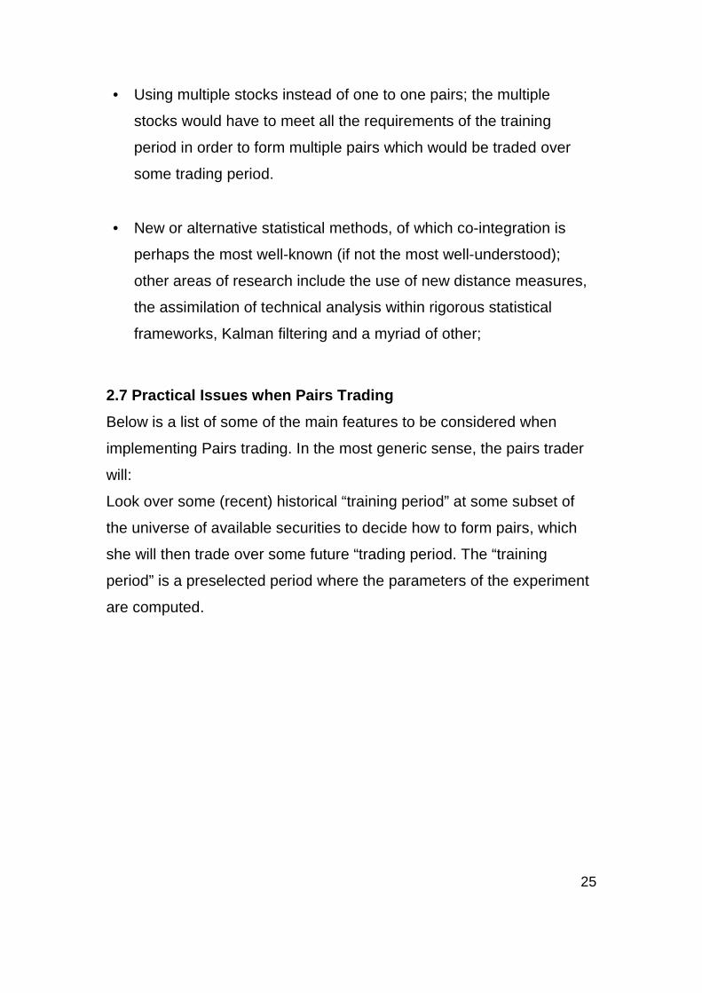
It is evident from Table 2 that the long positions are more profitable than

the short positions for daily, weekly and monthly periods. In addition, it

can be seen that the time period chosen was representative of a bull

market. This suggests that a long only fund would have been a suitable

strategy over the chosen time period. The returns were also positive in

the short positions for all thresholds in the daily and weekly frequencies

but lower than all the returns for the long positions across all its

corresponding thresholds in the daily and weekly frequencies. At the

monthly frequency the returns for the long positions were significantly

larger than the returns for the short positions with negative returns for

short positions between thresholds 1.7 and 2.4.

Table 2 :Pairs Trading Long and Short Postions

Threshold

Value Long Short Long Short Long Short

1.5 12.13% 5.26% 9.23% 7.46% 8.59% 1.96%

1.6 13.41% 8.14% 12.03% 10.82% 8.46% 1.64%

1.7 12.04% 8.51% 14.06% 10.52% 6.93% -2.64%

1.8 10.48% 8.42% 14.27% 10.73% 8.39% -3.36%

1.9 9.20% 8.12% 15.02% 11.73% 9.47% -5.35%

2 8.21% 7.23% 14.93% 10.52% 9.58% -3.58%

2.1 8.45% 5.82% 15.93% 12.82% 4.94% -3.78%

2.2 9.36% 6.34% 16.32% 13.92% 3.85% -4.85%

2.3 7.42% 4.21% 15.32% 14.24% 2.84% -3.84%

2.4 7.38% 6.32% 16.92% 13.73% 3.27% -3.74%

2.5 7.25% 5.21% 16.42% 13.63% 2.47% 0.24%

2.6 6.91% 4.72% 14.85% 10.54% 4.83% 1.65%

2.7 3.59% 2.43% 12.75% 9.34% 1.83% 2.63%

2.8 3.42% 2.32% 11.75% 7.27% 1.31% 0.67%

2.9 4.72% 2.19% 9.35% 2.62% 1.63% 0.54%

3 4.30% 1.56% 8.34% 4.26% 0.16% 0.32%

Daily Weekly Monthly

36

4.2 Risk Analysis

37

In order to obtain the alpha and beta coefficients, which is

representative of the risks associated with pairs trading, the portfolio

returns were regressed on the weighted index of the Top 40. Jenson’s

alpha or alpha as it is commonly called is a performance measure that

represents the average return on a portfolio over and above that

predicted by the CAPM model, given the portfolio’s beta and average

market return. If one has to choose between two trading strategies with

the same return, one would want to invest in the strategy that is less

risky. Jensen’s alpha can help one determine if they are earning the

right return for the level of risk for the strategy. Jensen’s alpha should

be positive and statistically significant if the strategy has performance

which cannot be explained by the market. Then the strategy would be

earning excessive returns.

38

From panels A, B and C we can see that the daily, weekly and monthly

returns have positive and significant alphas at all threshold values. We

can conclude that the pairs trading strategy has a positive abnormal

return after considering market factors.

The second coefficient in Table 2 is the pairs trading strategy’s Beta.

Beta is a measure of the volatility or systematic risk of a trading strategy

in comparison to the market as a whole. Beta can be thought of as

measure of a securities response to swings in the market. The higher

the beta of an asset the more correlated with the market it is i.e. the

greater its market risk and the more exposed it is to changes in the

market.

From Table 2, we can see that all the beta coefficients are small and

close to zero with none of them significant at daily, weekly and monthly

frequencies. This is an expected result and supports the concept of

pairs trading being a market neutral strategy i.e. its returns is not

dependent on market movements. Pairs trading involves the execution

of a long and short position at the same time which creates a natural

hedge against market movements.

4.3 Skill vs. Luck

The bootstrapping technique has become a standard when determining

the performance of investment strategies and the skill of investment

managers. The bootstrapping technique allows for a comparison of the

actual returns from a strategy or investment product against a series of

randomly generated returns. The idea is to test whether the returns

which are attributable to a strategy are due to skill or whether they were

39

arrived at by random chance or luck. By creating a synthetic portfolio

using random market entries and then saving the performance for each

simulation, the results can be tested against the performance of the

actual values. If the measures of performance that are attributed to the

strategy are not significantly different from those generated by random

signals (luck) then one may come to the conclusion that the strategies

return is not profitable.

According to Perlin (2006) , a percentage close to 90% would mean a

valuable strategy, 50% represents a case of chance and 10% means

the pairs trading strategy presents no value i.e. one can get more value

from random trading. At daily and weekly frequencies the returns due to

pairs trading are far superior to those which could be attributed to luck

with the strategy beating between 91% and 100% of the random

portfolios for each threshold value.

At the monthly frequency the evidence was not as conclusive for all

thresholds when taking into consideration transaction costs with most

thresholds above 50% (between 41% and 97%). It is reasonable to

conclude that random trading only beats the pairs trading strategy in a

few cases and thus a pairs trading strategy is superior to random

trading.

In the monthly frequency much fewer trades are created using the pairs

trading strategy and might not be entirely conclusive in assessing the

strategies performance.

.

40

Table 4: Pairs Trading Returns vesus Bootstrap

Threshold % Days in market No Trade Raw Ret % Randon Portfolio Beaten Raw Return TC % Random Portfolio Beaten

1.5 82.13% 7888 9.23% 100.00% -4.16% 100.00%

1.6 74.23% 6730 11.21% 100.00% -3.38% 100.00%

1.7 71.82% 5858 8.32% 100.00% -2.42% 100.00%

1.8 68.36% 5020 7.53% 100.00% -1.25% 100.00%

1.9 63.36% 4426 8.12% 100.00% 1.78% 100.00%

2 58.48% 3830 6.98% 100.00% 1.32% 100.00%

2.1 53.84% 3304 7.24% 100.00% 2.94% 100.00%

2.2 47.47% 2810 6.41% 100.00% 3.82% 100.00%

2.3 42.84% 2538 6.12% 100.00% 3.15% 100.00%

2.4 36.39% 2210 5.31% 100.00% 2.89% 100.00%

2.5 32.39% 1858 5.87% 100.00% 4.08% 100.00%

2.6 29.38% 1626 4.96% 100.00% 5.32% 96.00%

2.7 26.04% 1438 5.16% 100.00% 4.38% 94.30%

2.8 22.70% 1258 4.34% 100.00% 3.73% 100.00%

2.9 17.94% 1076 4.75% 100.00% 5.96% 100.00%

3 13.85% 912 3.68% 100.00% 3.87% 100.00%


1.5 82.39% 3056 9.65% 100.00% 5.47% 100.00%

1.6 76.48% 2758 9.12% 100.00% 8.52% 100.00%

1.7 72.48% 2635 10.14% 100.00% 10.27% 100.00%

1.8 71.49% 2320 11.13% 100.00% 11.18% 100.00%

1.9 68.38% 2290 12.34% 100.00% 12.05% 100.00%

2 63.94% 2135 13.28% 100.00% 10.64% 100.00%

2.1 59.18% 1959 14.38% 100.00% 12.93% 100.00%

2.2 54.56% 1627 12.64% 100.00% 11.93% 100.00%

2.3 51.44% 2175 13.54% 100.00% 11.86% 98.90%

2.4 48.27% 1290 14.39% 100.00% 13.76% 93.60%

2.5 43.39% 1142 12.96% 100.00% 11.37% 100.00%

2.6 39.59% 876 11.94% 100.00% 9.86% 100.00%

2.7 32.39% 867 8.29% 98.50% 9.38% 92.20%

2.8 27.39% 691 8.17% 97.20% 8.37% 95.30%

2.9 24.25% 627 7.25% 95.20% 7.98% 91.60%

3 19.32% 621 7.87% 100.00% 7.49% 100.00%


1.5 82.47% 697 5.24% 100.00% 3.45% 90.60%

1.6 78.23% 628 5.19% 100.00% 2.87% 90.80%

1.7 68.62% 581 4.25% 100.00% 0.45% 80.60%

1.8 65.29% 495 4.26% 100.00% 2.16% 72.80%

1.9 62.18% 413 3.98% 100.00% 1.31% 65.80%

2 58.28% 295 2.18% 100.00% 0.78% 40.60%

2.1 41.39% 223 2.47% 82.60% 1.34% 78.60%

2.2 34.29% 167 2.05% 78.50% 0.85% 72.50%

2.3 26.48% 186 1.75% 98.60% -0.95% 74.80%

2.4 21.48% 107 1.70% 100.00% -0.59% 79.50%

2.5 15.85% 88 2.76% 100.00% -1.08% 54.30%

2.6 13.35% 50 2.84% 87.20% 0.68% 40.90%

2.7 10.58% 21 1.34% 79.40% 0.23% 65.40%

2.8 7.49% 21 0.49% 82.50% -0.14% 70.40%

2.9 6.37% 7 1.28% 100.00% 0.31% 97.40%

3 2.52% 8 1.59% 90.30% 0.17% 67.30%

Panel A - Daily Frequency

Panel B - Weekly Frequency

Panel C - Weekly Frequency

41

5. CHAPTER 5: Conclusions and Recommendations

The best raw returns were found to be at the weekly frequency whilst

the daily and monthly frequency was also profitable before taking into

transaction costs. Frequency refers to how often trading occurs i.e.

either on a daily, weekly or monthly basis. After taking into account

transaction costs, the weekly raw returns were still positive for all

thresholds whilst the daily returns were positive for thresholds greater

than 1.8 and for monthly returns with transaction costs all the returns

were positive for thresholds less than 2.3. For the daily raw returns with

transaction costs, the high transaction costs for emerging market equity

exchanges, could explain the negative returns for thresholds less than

1.9.

The evidence of a bull market is clearly visible as the returns from the

long positions are greater than the short positions for all the frequencies

and for almost all the thresholds.

The results also shows that the intellectual capital used in the trading

strategy would outperform random trading as illustrated by the

comparison against the bootstrap method.

The time period for the data also took into consideration the financial

crisis period of 2008-2009. The results also shows that the pairs trading

strategy remained profitable through the financial crisis and that the

notion that a pairs trading strategy is market neutral is sound.

Interesting further studies using pairs trading could be done across

asset classes in South Africa, especially with commodity instruments. It

would also be interesting to conduct this research on South Africa’s

highly developed derivatives market.

42

References

[1] Acharya, V. and L. Pedersen (2005). “Asset pricing with liquidity risk”.

Journal of Financial Economics 77 (2): 375-385.

[2] Agarwal, V. and N. Naik (2004). “Risks and portfolio decisions involving

hedge funds.” Review of Financial Studies 17 (1): 63-71.

[3] Ali, A., and M. Trombley (2004). “Short sale constraints and momentum in

stock returns.” Working paper, University of Arizona.

[4] Amihud, Y. (2002). “Illiquidity and stock returns: Cross-section and time-

series effects.” Journal of Financial Markets 5 (1): 31-35.

[5] Andrade, S., V. Di Pietro., and M. Seasholes. (2005). “Understanding the

profitability of pairs trading”, UC Berkeley Haas School Working Paper

[6] Ball, R, S.P. Kothari, C. Wasley (1995). “Can we implement research on

stock trading rules?” The Journal of Portfolio Management 21 (Winter): 54-63.

[7] Bertram, W.K. (2010). “Analytic solutions for optimal statistical arbitrage

trading”. Physica A, 389: 2234-2243.

[8] Bris, A., W. N. Goetzmann, and N. Zhu. (2007). “Efficiency and the Bear:

Short-Sales and Markets around the World.” The Journal of Finance 62(3):

1029-1079.

43

[9] Brooks, C., A. Katsaris and, G. Persand. (2005) “Timing is everything: A

Comparison and Evaluation of Market Timing Strategies” Working Paper,

Available at SSRN: http://ssrn.com/abstract=834485.

[10] Caldeira, J.F. and G.V. Moura. (2013). “Selection of a Portfolio of Pairs

Based on Co-integration: A Statistical Arbitrage Strategy”. Brazilian Review of

Finance, 11:49–80.

[11] Carhart, M. (1997). “On Persistence in Mutual Fund Performance.”

Journal of Finance 52: 57-82.

[12] Chang, M.T. (2007). “Understanding the risks in and rewards for pairs-

trading”, June 2007, ICBME.

[13] Chen, Z. and P. J. Knez. (1995). “Measurement of market integration and

arbitrage.” Review of Financial Studies 8(2):287-325.

[14] DeBondt, W. F. M. and R. Thaler. (1985). “Does the Stock Market

Overreact?” Journal of Finance 40, 793-805.

[15] Do, B. and R. Faff. (2009). “Does naïve pairs trading still work?”, Working

Paper, Monash University

[16] Do, B., R. Faff., and K. Hamza. (2006). “A new approach to modelling and

estimation for pairs trading”, Working Paper, Monash University.

44

[17] Dunis, C.L., G. Giorgini, J. Laws, and J. Rudy. (2010). “Statistical arbitrage

and high-frequency data with an application to Eurostoxx 50 equities.”

Working Paper, Liverpool Business School.

[18] Elliott, R., J. van der Hoek, and W. Malcolm. (2005). “Pairs Trading.”

Quantitative Finance 5(3): 271-276.

[19] Erhman, D.S., 2006, “The Handbook of Pairs Trading: Strategies Using

Equities, Options and Futures.” John Wiley & Sons Inc.

[20] Fama, E. F. (1970). “Efficient capital markets: A review of theory and

empirical work.” Journal of Finance 25(2):383-418.

[21] Fung, W., and D Hsieh. (2004). “Hedge Fund Benchmarks: A Risk-Based

Approach.” Financial Analysts Journal 60:65-80.

[22] Gatev, E., W. N. Goetzmann, and K. G. Rouwenhort. (1999). “Pairs

Trading: Performance of a Relative Value Arbitrage Rule.” Working Paper, Yale

School of Management. Available at SSRN: http://ssrn.com/abstract=141615.

[23] Ingersoll, I. (1987). “Theory of Financial Decision-Making.” Rowman and

Littlefield, Totowa, NJ.

[24] Jylha, P., K. Rinne, and M. Suominen. (2010). “Do Hedge Funds Supply or

Demand Liquidity?” working paper, Aalto University.

45

[25] Lamont, O. A., and R.H. Thaler. (2003). “Anomalies: The law of one price

in financial markets.” Journal of Economic Perspectives 17(4):191-202.

[26] Lo, A.W. (2008). “Hedge Funds: An Analytic Perspective.” Princeton, NJ:

Princeton University Press.

[27] Marshall, B.R., R.H. Cahan, and J.M. Cahan. (2008). “Can commodity

futures be profitably traded with quantitative market timing strategies?

Working paper.

[28] Perlin, M S. (2006). “Evaluation of Pairs Trading Strategy at Brazilian

Financial Market.” Working Paper, http://ssrn.com/abstract=952242.

[29] Perlin, M. (2007). “M of a kind: A multivariate approach at pairs trading.”

Working paper.

[30] Politis, D., and J. Romano. (1994). “The Stationary Bootstrap.” Journal of

the American Statistical Association 89:428

[31] Purnendu, Nath, (2003). “High Frequency Pairs Trading with U.S. Treasury

Securities: Risks and Rewards for Hedge Funds.” Working Paper, London

Business School.

[32] Sarr, A., and T. Lybek. (2002). “Measuring liquidity in financial markets.”

Working paper, 2002.

46

[33] Shleifer, A., and R. Vishny. (1997). “The limits of arbitrage.” Journal of

Finance 52:35-55.

[34] Stulz, R. (2007). “Hedge Funds: Past, Present and Future.” Journal of

Economic Perspectives 21:175-194.

[35] Vidyamurthy, G. (2004). “Pairs Trading: Quantitative Methods and

Analysis” John Wiley &Sons, 2004

[36] Whistler, M. (2004). “Pairs trading: capturing profits and hedging risk with

statistical arbitrage strategies.” Hoboken, NJ: Wiley.

47

APPENDIX A – Share codes used for pairs trading

Table 5: List of share codes used

JSE Share Code Company

ABL African Bank Inv Ltd

ACL ArcelorMittal SA Limited

ACT AfroCentric Inv Corp Ltd

ADH ADvTECH Ltd

ADR Adcorp Holdings Limited

AFE AECI Limited

AFR Afrgri LTD

AFX African Oxygen Limited

AGL Anglo American plc

ALT Allied Technologies LTD

AMA Home of Living Brands holding Limited

AME African Media Ent Ltd

AMS Anglo American Plat Ltd

AND Andulela Inv Hldgs Ltd

AOO African & Over Ent Ltd

APK Astrapak Limited

APN Aspen Pharmacare Hldgs Ltd

ARI African Rainbow Min Ltd

ART Argent Industrial Ltd

ASA ABSA GROUP LTD

ASR Assore Ltd

ATN Allied Electronics Corp LTD

AVI AVI Ltd

AWT Awethu Breweries Ltd

BAT Brait SE

BAU Bauba Platinum Limited

BAW Barloworld Ltd

BCF Bowler Metcalf Ltd

BDM Buildmax Ltd

BEG Beige Holdings LTD

BEL Bell Equipment Ltd

BIL BHP Billiton plc

BSR Basil Read Holdings Ltd

48


BVT Bidvest Ltd

CAP Cape empowerment LTD

CAT Caxton CTP Publish Print

CFR Compagnie Fin Richemont

CKS Crookes Brothers Ltd

CLH City Lodge Hotels Ltd

CLS Clicks Group Ltd

CMH Combined Motor Hldgs Ltd

CNL Control Investments Group Limited

CPL Capital Property Fund

CRG Cargo Carriers Ltd

CRM Ceramic Industries LTD

CSB Cashbuild Ltd

CUL Cullinan Holdings Ltd

CVI Capevin Investments LTD

DAW Distr and Warehousing

DLV Dorbyl Limited

DON The Don Group Limited

DRD DRD Gold Ltd

DST Distell Group Ltd

DTA Delta EMD Ltd

DTC Datatec Ltd

EHS Evraz Highveld Steel & Van

ELR ELB Group Ltd

FBR Famous Brands Ltd

FPT Fountainhead Property Trust

FSR Firstrand Ltd

GFI Gold Fields Ltd

GGM Goliath Gold Mining Ltd

GND Grindrod Ltd

GRF Group Five Ltd

GRT Growthpoint Prop Ltd

HAR Harmony GM Co Ltd

HDC Hudaco Industries Ltd

HWN Howden Africa Hldgs Ltd

HYP Hyprop Inv Ltd

IFH IFA Hotels & Resorts Limited

ILV Illovo Sugar Ltd

IMP Impala Platinum Hlgs Ltd

INL Investec Ltd

IPL Imperial Holdings Ltd

ITE Italtile Ltd

IVT Invicta Holdings Ltd

49


JDG JD GROUP LIMITED

JSC Jasco Electron Hldgs Ltd

KAP KAP Industrial Hldgs Ltd

KGM Kagiso Media Limited

LAB Labat Africa Limited

LBH Liberty Holdings Ltd

LNF London Fin Inv Group plc

LON Lonmin plc

MAS Masonite Africa Ltd

MDC Mediclinic Internat Ltd

MFL Metrofile Holdings Ltd

MPC MR PRICE GROUP LIMITED

MRF Merafe Resources Ltd

MST Mustek Ltd

MTA Metair Investments Ltd

MTN MTN Group Ltd

MUR Murray & Roberts Hldgs

MVG Mvelaphanda Group Limited

NCS Nictus Ltd

NED Nedbank Group Ltd

NHM Northam Platinum Ltd

NPK Nampak Ltd

NPN Naspers Ltd -N-

NTC Netcare Limited

NWL Nu-world Holdings Limited

OCE Oceana Group Ltd

OCT Octodec Invest Ltd

OMN Omnia Holdings Ltd

PBT PBT group Limited

PET Petmin Ltd

PIK Pick n Pay Stores Ltd

PMM Premium Properties Limited

PNC Pinnacle Hldgs Ltd

PPC PPC Limited

PPR Putprop Ltd

PSG PSG Group Ltd

PWK Pick N Pay Holdings Ltd

QPG Quantum Property Group

RBW Rainbow Chicken Limited

RLO Reunert Ltd

RMH RMB Holdings Ltd

50


RNG Randgold & Expl Co Ltd

RTN Rex Trueform Cl Co -N-

RTO Rex Trueform Cloth Co Ld

SAB SABMiller plc

SAC SA Corp Real Estate Ltd

SAP Sappi Ltd

SBK Standard Bank Group Ltd

SBL Sable Holdings Limited

SBV Sabvest Ltd

SCL Sacoil Holdings Ltd

SER Seardel Inv Corp Ltd

SHP Shoprite Holdings Ltd

SIM Simmer and Jack Mines Limited

SLO Southern Electricity Company Limited

SNT Santam Limited

SNU Sentula Mining Ltd

SOL Sasol Limited

SOV Sovereign Food Inv Ltd

SPA Spanjaard Limited

SUI Sun International Ltd

SYC Sycom Property Fund

TBS Tiger Brands Ltd

TFG The Foschini Group Limited

TMT Trematon Capital Inv Ltd

TON Tongaat Hulett Ltd

TON Tongaat Hulett Ltd

TPC Transpaco Ltd

TRE Trencor Ltd

TSH Tsogo Sun Holdings Ltd

TSX Trans Hex Group Ltd

VIL Village Main Reef Ltd

WBO Wilson Bayly Hlm-Ovc Ltd

WHL Woolworths Holdings Ltd

WNH Winhold Ltd

YRK York Timber Holdings Ltd

ZCI ZCI Limited

ZSA Zurich Insurance Company SA

Documents

Evaluation of the performance of a pairs trading strategy