Annals of Mathematics 175 (2012), 977–1000http://dx.doi.org/10.4007/annals.2012.175.2.11

Evaluation of the multiple zeta valuesζ(2, . . . , 2, 3, 2, . . . , 2)

By D. Zagier

Abstract

A formula is given for the special multiple zeta values occurring in the

title as rational linear combinations of products ζ(m)π2n with m odd. The

existence of such a formula had been proved using motivic arguments by

Francis Brown, but the explicit formula (more precisely, certain 2-adic prop-

erties of its coefficients) were needed for his proof in [2] of the conjecture

that all periods of mixed Tate motives over Z are Q[(2πi)±1]-linear com-

binations of multiple zeta values. The formula is proved indirectly, by

computing the generating functions of both sides in closed form (one as the

product of a sine function and a 3F2-hypergeometric function, and one as

a sum of 14 products of sine functions and digamma functions) and then

showing that both are entire functions of exponential growth and that they

agree at sufficiently many points to force their equality. We also show that

the space spanned by the multiple zeta values in question coincides with

the space of double zeta values of odd weight and find a relation between

this space and the space of cusp forms on the full modular group.

1. Introduction and statement of results

Multiple zeta values are real numbers, originally defined by Euler, that

have been much studied in recent years because of their many surprising prop-

erties and the many places they appear in mathematics and mathematical

physics, ranging from periods of mixed Tate motives to values of Feynman

integrals in perturbative quantum field theory. There are many conjectures

concerning the values of these numbers. Two of the most interesting were

proved very recently by Francis Brown [2] (see also [1]), but for the proofs he

needed to have explicit formulas expressing the specific multiple zeta values

indicated in the title in terms of values of the Riemann zeta function. It is the

purpose of this note to give these formulas and their proof.

We first give the definition and formulations of some of the main conjec-

tures concerning multiple zeta values (henceforth usually abbreviated MZV’s)

and then indicate the statements of the results that we will prove. For pos-

itive integers k1, . . . , kn with kn ≥ 2, we define the MZV ζ(k1, . . . , kn) as the

977

978 D. ZAGIER

iterated multiple sum

(1) ζ(k1, . . . , kn) =∑

0<m1<···<mn

1

mk11 · · ·m

knn

.

(Many papers use the opposite convention, with the mi’s ordered by m1 >

· · · > mn > 0, but (1) will be more convenient for us.) These series usually

converge quite slowly, but they can be rewritten in several different ways that

allow their rapid calculation to high precision. I performed such computations

a number of years ago (they were later extended much further) and found that

the MZV’s of a given weight k = k1 + · · · + kn satisfy many numerical linear

relations over Q, e.g., of the 210 = 1024 MZV’s of weight 12, only 12 were

linearly independent. The numerical data suggested the conjecture that the

dimension of the Q-vector space Zk spanned by all MZV’s of weight k is given

by

(2) dimZk?= dk,

where dk is defined as the coefficient of xk in the power series expansion of1

1−x2−x3 (or equivalently by the recursion dk = dk−2 + dk−3 with the initial

conditions d0 = 1 and dk = 0 for k < 0). Proving this conjecture is hopeless at

the present time; indeed, there is not a single value of k for which it is known

that dimZk > 1. (In particular, the irrationality of ζ(k1, . . . , kn)/πk1+···+kn

is not known for a single value of the vector (k1, . . . , kn). Nor is it known—

although it is surely true—that the different subspaces Zk of R are disjoint,

so that the sum Z =∑k Zk is direct.) However, the true MZV’s in R are the

images under a Q-linear map of certain “motivic” MZV’s which are defined

purely algebraically, and it was proved (independently) by Terasoma [10] and

Goncharov [6], [3] that the upper bound implied by the conjectural dimension

formula held for these, implying in particular the inequality

(3) dimZk ≤ dk.

Now it is clear that dk can also be defined as the number of MZV’s of

weight k all of whose arguments are 2’s and 3’s, and M. Hoffman [7] made

the conjecture that these special MZV’s span Zk. This statement refines (3),

and also implies, if one believes the conjecture (2), that the MZV’s in question

form a Q-basis of Zk for all k.

In a different direction, Terasoma and Goncharov established (3) by show-

ing that all MZV’s are periods of mixed Tate motives that are unramified

over Z, and another well-known conjecture in the area states the converse, i.e.,

that all periods of mixed Tate motives over Z can be expressed as linear combi-

nations (over Q[(2πi)−1]) of MZV’s. Equivalently, this says that the dimension

of the space of motivic MZV’s of weight k is equal to dk.

EVALUATION OF THE MULTIPLE ZETA VALUES ζ(2, . . . , 2, 3, 2, . . . , 2) 979

The result obtained by Francis Brown was a proof of both of these two

conjectures, assuming certain quite specific properties of certain coefficients

occurring in the relations over Q of some special MZV’s. Specifically, he showed

that the special MZV’s

(4) H(a, b) := ζ(2, . . . , 2︸ ︷︷ ︸a

, 3, 2, . . . , 2︸ ︷︷ ︸b

) (a, b ≥ 0),

which are part of Hoffman’s conjectural basis, are Q-linear combinations of

products π2m ζ(2n+ 1) with m+n = a+ b+ 1. His proof, which used motivic

ideas, did not yield an explicit formula for these linear combinations, but nu-

merical evidence suggested several properties satisfied by their coefficients (in

particular, that of the coefficient of ζ(2a+ 2b+ 3)) which he could show were

sufficient to imply the truth of both Hoffman’s conjecture and the statement

about motivic periods. In this paper we will state and prove an explicit formula

expressing the numbers (4) in terms of Riemann zeta values and confirming

the numerical properties that were required for Brown’s proof.

Before giving the formula for the numbers H(a, b), we first recall the much

easier formula

(5) H(n) := ζ(2, . . . , 2︸ ︷︷ ︸n

) =π2n

(2n+ 1)!(n ≥ 0)

for the simplest of the Hoffman basis elements. The proof of (5) is well known,

but we give it anyway, both for completeness and because similar ideas will be

used below: one simply forms the generating function∑∞n=0(−1)nH(n)x2n+1

and then, directly from the definition of H(n), finds

(6)∞∑n=0

(−1)nH(n)x2n+1 = x∞∏m=1

Ç1− x2

m2

å=

sinπx

π=∞∑n=0

(−1)nπ2n x2n+1

(2n+ 1)!,

the last two equalities both being due to Euler. Using (5), one can refor-

mulate the above statement about the expression of the numbers H(a, b) in

terms of powers of π2 and values of the Riemann zeta function at odd argu-

ments by saying that each H(a, b) is a rational linear combination of products

H(m) ζ(2n + 1) with m + n = a + b + 1. (It is in fact in this form that the

above-mentioned non-explicit formula was proved by Brown.) It turns out that

the coefficients in this new expression are simpler than those in terms of either

the products π2mζ(2n + 1) or ζ(2m)ζ(2n + 1). These coefficients were first

guessed on the basis of numerical data for weights up to 13, obtained using

the numerical algorithms mentioned above. We give this data (initially only

known to be true numerically, but to very high precision) and then state the

980 D. ZAGIER

general formula which it suggests:Ñζ(3, 2)

ζ(2, 3)

é=

Ñ92 −2

−112 3

éÑζ(5)

ζ(2) ζ(3)

é,Ü

ζ(3, 2, 2)

ζ(2, 3, 2)

ζ(2, 2, 3)

ê=

Ü−291

16 12 −2758 −11

2 015716 −15

2 3

êÜζ(7)

ζ(2) ζ(5)

ζ(2, 2) ζ(3)

ê,â

ζ(3, 2, 2, 2)

ζ(2, 3, 2, 2)

ζ(2, 2, 3, 2)

ζ(2, 2, 2, 3)

ì=

â64116 −30 12 −245516 −291

16 2 0

−88916

2998 −15

2 0

−22316

18916 −15

2 3

ìâζ(9)

ζ(2) ζ(7)

ζ(2, 2) ζ(5)

ζ(2, 2, 2) ζ(3)

ì,

ζ(3, 2, 2, 2, 2)

ζ(2, 3, 2, 2, 2)

ζ(2, 2, 3, 2, 2)

ζ(2, 2, 2, 3, 2)

ζ(2, 2, 2, 2, 3)

=

−17925256 56 −30 12 −2

−1153564

198516 −30 2 0

10689128 −889

1615716 0 0

958564 −1753

163158 −15

2 04603256 −255

1618916 −15

2 3

ζ(11)

ζ(2) ζ(9)

ζ(2, 2) ζ(7)

ζ(2, 2, 2), ζ(5)

ζ(2, 2, 2, 2) ζ(3)

,

ζ(3, 2, 2, 2, 2, 2)

ζ(2, 3, 2, 2, 2, 2)

ζ(2, 2, 3, 2, 2, 2)

ζ(2, 2, 2, 3, 2, 2)

ζ(2, 2, 2, 2, 3, 2)

ζ(2, 2, 2, 2, 2, 3)

=

55299512 −90 56 −30 12 −2

281655512 −102405

256 140 −30 2 067683256 −11535

6464116 −2 0 0

−151965256

52929128 −1753

1618916 0 0

−157641512

1521764 −1785

163158 −15

2 0

−11261512

5115256 −255

1618916 −15

2 3

ζ(13)

ζ(2) ζ(11)

ζ(2, 2) ζ(9)

ζ(2, 2, 2) ζ(7)

ζ(2, 2, 2, 2) ζ(5)

ζ(2, 2, 2, 2, 2) ζ(3)

.

In these formulas one immediately sees certain patterns—all denominators are

powers of 2, many of the entries are zero, the northeast and southeast corners of

the matrices stabilize, etc.—and looking sufficiently carefully at the coefficients

one is finally led to guess the complete formula given in the following theorem.

EVALUATION OF THE MULTIPLE ZETA VALUES ζ(2, . . . , 2, 3, 2, . . . , 2) 981

Theorem 1. For all integers a, b ≥ 0, we have

(7)

H(a, b)=2a+b+1∑r=1

(−1)rñÇ

2r

2a+ 2

å−Å

1− 1

22r

ãÇ2r

2b+ 1

åôH(a+b−r+1)ζ(2r+1),

where the value of H(a+ b− r + 1) is given by (5). Conversely, each product

H(m)ζ(k − 2m) of odd weight k is a rational linear combination of numbers

H(a, b) with a+ b = (k − 3)/2.

Remark. The expressions for the products H(m)ζ(k− 2m) as linear com-binations of the numbers H(a, b) do not seem to have coefficients that can begiven by any simple formula. For example, the inverse of the 5 × 5 matrixgiven above expressing the vector {H(a, b) | a+ b = 4} in terms of the vector{ζ(2a+ 3)H(b) | a+ b = 4} is

1

2555171

à450607872 750355968 819546624 620662272 300405248

742409280 1236102000 1349936640 1022542528 494939520

369002592 613537008 669540272 508012288 246001728

89977320 147349978 160083660 122931470 59984880

15331307 22114173 23488575 19354609 11072595

í,

in which no simple pattern can be discerned and in which even the denomi-

nator (here prime) cannot be recognized. This shows that the Hoffman basis,

although it works over Q, is very far from giving a basis over Z of the Z-lattice

of MZV’s, and suggests the question of finding better basis elements.

Theorem 1 (together with the identity (5)) tells us that for each odd weight

k = 2K+1, the numbers H(a,K − 1− a) (0 ≤ a ≤ K−1) and ζ(2r+1)π2K−2r

(1 ≤ r ≤ K) span the same vector space over Q (and hence presumably each

give a basis for this space, since the numbers ζ(2r + 1)/π2r+1 are believed to

be linearly independent over Q). This same space has yet another description

as the space spanned by the double zeta values ζ(m,n) with m+n = k, as was

essentially proved by Euler. The number of these double zeta values, together

with ζ(k) itself (which is known to be the sum of all of them), equals 2K.

Thus these numbers cannot form a basis, but the set of all of them splits up

naturally into two subsets of K elements each:

(a) ζ(k) and ζ(2r, k − 2r) (r = 1, . . . ,K − 1),

(b) ζ(2r + 1, k − 2r − 1) (r = 0, . . . ,K − 1),

and we can ask whether each of these sets already spans (and therefore is a

conjectural base of) the space in question. The answer is given in the following

two theorems, which will be proved in Section 5 and Section 6, respectively.

Theorem 2. For each odd integer k = 2K + 1 ≥ 3, the K numbers

(a) span the same space as the K numbers {H(a, b) | a + b = K − 1} or

{π2rζ(k − 2r) | 0 ≤ r ≤ K − 1}.

982 D. ZAGIER

Theorem 3. For each odd integer k = 2K + 1 ≥ 5, the numbers (b)

satisfy [(K − 5)/3] relations over Q.

The number [(K − 5)/3] = [(k − 11)/6] in this theorem actually arises as

dimSk−1 + dimSk+1, where Sh denotes the space of cusp forms of weight h on

the full modular group SL(2,Z). (More precisely, it arises as the sum of the

dimensions of the space of odd period polynomials of weight k − 1 and even

period polynomials of weight k + 1, but it is well known that these spaces of

period polynomials are isomorphic to the space of cusp forms on SL(2,Z).)

This connection is interesting both in itself and because of the relation to the

results of [5], in which various relations were made between double zeta values

ζ(a, b) of even weight a + b = k and cusp forms (resp. even or odd period

polynomials) of the same weight.

Finally, in Section 7 of the paper we prove the analogue of Theorem 1 for

the Hoffman “star” elements H∗(a, b) (defined like H(a, b) but using “multiple

zeta-star values,” i.e., by allowing equality among the mi’s in (1)), by showing

that their generating function is a simple multiple of the generating function

of the H(a, b)’s. As a corollary, we obtain a recent result of Ihara, Kajikawa,

Ohno and Okuda [8] showing that all odd zeta values ζ(2K+1) are very simple

linear combinations of the numbers H∗(a,K−1−a), unlike the situation for the

usual Hoffman elements, where, as we just saw, the corresponding coefficients

can apparently not be given in closed form.

2. The generating functions of H(a, b) and “H(a, b)

Our strategy to prove the theorem is to study the two generating functions

F (x, y) =∑a, b≥0

(−1)a+b+1H(a, b)x2a+2 y2b+1,(8) “F (x, y) =∑a, b≥0

(−1)a+b+1“H(a, b)x2a+2y2b+1,(9)

where “H(a, b) denotes the expression occurring on the right-hand side of (7). In

this section we will compute each of these generating functions in terms of clas-

sical special functions (Propositions 1 and 2). If the two expressions obtained

were the same, we would be done, but in fact they are completely different, one

involving a higher hypergeometric function and the other a complicated linear

combination of digamma functions. We therefore have to proceed indirectly,

showing that both F and “F are entire functions of order 1 in x and y and that

they agree whenever x = y or x or y is an integer. This will imply the equality

F = “F and hence H = “H.

We begin with F (x, y). Recall that the hypergeometric function

pFp−1

Ça1, . . . , apb1, . . . , bp−1

∣∣∣∣xå

EVALUATION OF THE MULTIPLE ZETA VALUES ζ(2, . . . , 2, 3, 2, . . . , 2) 983

is defined as∑∞m=0

(a1)m···(ap)m(b1)m···(bp−1)m

xm

m! , where (a)m = a(a + 1) · · · (a + m − 1)

denotes the ascending Pochhammer symbol.

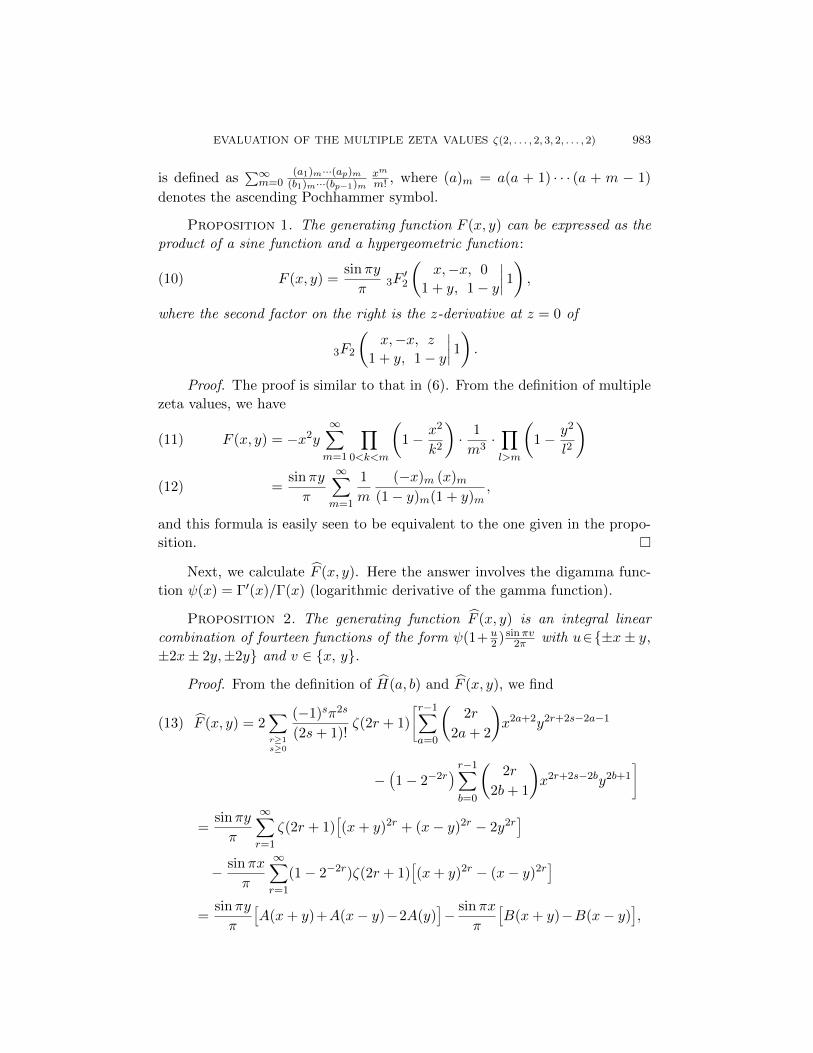
Proposition 1. The generating function F (x, y) can be expressed as the

product of a sine function and a hypergeometric function :

(10) F (x, y) =sinπy

π3F′2

Çx,−x, 0

1 + y, 1− y

∣∣∣∣ 1å,

where the second factor on the right is the z-derivative at z = 0 of

3F2

Çx,−x, z

1 + y, 1− y

∣∣∣∣ 1å.

Proof. The proof is similar to that in (6). From the definition of multiple

zeta values, we have

F (x, y) = −x2y∞∑m=1

∏0<k<m

Ç1− x2

k2

å· 1

m3·∏l>m

Ç1− y2

l2

å(11)

=sinπy

π

∞∑m=1

1

m

(−x)m (x)m(1− y)m(1 + y)m

,(12)

and this formula is easily seen to be equivalent to the one given in the propo-

sition. �

Next, we calculate “F (x, y). Here the answer involves the digamma func-

tion ψ(x) = Γ′(x)/Γ(x) (logarithmic derivative of the gamma function).

Proposition 2. The generating function “F (x, y) is an integral linear

combination of fourteen functions of the form ψ(1+ u2 ) sinπv2π with u∈{±x± y,

±2x± 2y,±2y} and v ∈ {x, y}.

Proof. From the definition of “H(a, b) and “F (x, y), we find“F (x, y) = 2∑r≥1s≥0

(−1)sπ2s

(2s+ 1)!ζ(2r + 1)

ñr−1∑a=0

Ç2r

2a+ 2

åx2a+2y2r+2s−2a−1(13)

−Ä1− 2−2r

ä r−1∑b=0

Ç2r

2b+ 1

åx2r+2s−2by2b+1

ô=

sinπy

π

∞∑r=1

ζ(2r + 1)î(x+ y)2r + (x− y)2r − 2y2r

ó− sinπx

π

∞∑r=1

(1− 2−2r)ζ(2r + 1)î(x+ y)2r − (x− y)2r

ó=

sinπy

π

îA(x+ y)+A(x− y)−2A(y)

ó− sinπx

π

îB(x+ y)−B(x− y)

ó,

984 D. ZAGIER

where A(z) and B(z) denote the power series

(14) A(z) =∞∑r=1

ζ(2r + 1) z2r, B(z) =∞∑r=1

(1− 2−2r) ζ(2r + 1) z2r.

These series converge only for |z| < 1, but if we rewrite them as

(15) A(z) =∞∑n=1

z2

n (n2 − z2), B(z) =

∞∑n=1

(−1)n−1z2

n (n2 − z2),

then the new series converge for all z and define meromorphic functions of z

in the whole complex plane, with simple poles only at z ∈ Z r {0}. We can

also write them in terms of the digamma function ψ(x) = Γ′(x)/Γ(x) by the

formulas

A(z) =1

2

∞∑n=1

Å1

n− z+

1

n+ z− 2

n

ã= ψ(1)− 1

2(ψ(1 + z) + ψ(1− z)) ,

B(z) =1

2

∞∑n=1

(−1)n−1Å

1

n− z+

1

n+ z− 2

n

ã= A(z)−A(z/2).

(16)

Substituting (16) into (13) gives an expression for “F of the form stated in the

proposition. �

As explained above, the expressions for F and “F in these two propositions

are very different, and the proof of their equality will proceed in an indirect

manner. For this purpose we will need the analytic properties of both functions

as given in the following proposition.

Proposition 3. Both F (x, y) and “F (x, y) are entire functions on C×Cand are bounded by a constant multiple of eπX logX as X → ∞, where X =

max{|x|, |y|}, and also by a multiple (depending on x) of eπ|=(y)| as |y| → ∞with x ∈ C fixed.

Proof. For F (x, y), the first two statements follow from the estimate

0 < H(a, b) <1

a+ 1H(n) =

1

a+ 1

π2n

(2n+ 1)!(a+ b+ 1 = n),

which implies the convergence of the series in (8) for all x, y ∈ C and gives the

majorization

(17) max|x|, |y|≤M

|F (x, y)| <∞∑n=1

Å1 +

1

2+ · · · 1

n

ãπ2nM2n+1

(2n+ 1)!= O

ÄeπM logM

ä.

For the third statement, we note that it suffices to prove the desired estimate

(18) |F (x, y)| = Ox

Äeπ|=(y)|

ä,

EVALUATION OF THE MULTIPLE ZETA VALUES ζ(2, . . . , 2, 3, 2, . . . , 2) 985

for (say) |=(y)| ≥ 2, because then the Phragmen-Lindelof theorem together

with the fact that F (x, y) is a function of order 1 with respect to y (by esti-

mate (17)) imply the same estimate within the strip. But if |=(y)| ≥ 2, then

an easy estimate gives |(1 − y)m(1 + y)m| > m!2 for all m ≥ 1, and since

(−x)m(x)m = Ox((m− 1)!2) this means that the sum in (12) is majorized by

a multiple (depending on x) of the convergent sum∑mm

−3, establishing the

desired estimate (18).

For “F (x, y), the holomorphy follows from (13) and (15) or (16): the latter

equations show that the only singularities of A(z) and B(z) are simple poles

at z ∈ Z with residues given by

(19)

Resz=nA(z) = −sgn n

2, Resz=nB(z) = (−1)n

sgn n

2(n ∈ Z),

so the potential poles in (13) when y ∈ Z are canceled by the zeros of sinπy

and the potential poles when x ± y = n ∈ Z cancel because the residues of

A(x ± y) and ±B(x ± y) differ by a factor ∓(−1)n and the coefficients sinπxπ

and sinπyπ differ by the same factor. Finally, both majorizations

(20) max|x|, |y|≤M

|“F (x, y)| = OÄeπM logM

äand

(21) |“F (x, y)| = Ox

Äeπ|=(y)|

äfollow from the easy estimate1 ψ(x) = O(log x) + O(1/dist(x,Z)). �

3. Special values of F (x, y) and “F (x, y)

In the next three propositions we verify the equality of the two functions

F and “F for various special values of their arguments.

Proposition 4. For x ∈ C, we have

(22) F (x, x) = −sinπx

πA(x) = “F (x, x),

where A(z) is the meromorphic function defined by equation (14), (15) or (16).

Corollary. For n ≥ 1, we have the identity

(23) ∑a+b+1=n

H(a, b) =∑

a+b+1=n

“H(a, b) =n∑r=1

(−1)r−1π2n−2r

(2n− 2r + 1)!ζ(2r + 1).

1Use the standard estimate ψ(x) = log(x) + O(1/x) in the half-plane <(x) ≥ 0 and the

functional equation ψ(x)−ψ(1−x) = π cotπx = O(1)+O(1/dist(x,Z)) for x in the half-plane

<(x) ≤ 0.

986 D. ZAGIER

Proof. From (12) and (15) we immediately find

F (x, x) =sinπx

π

∞∑m=1

1

m· −x−x+m

· x

x+m= −sinπx

πA(x),

while from (13) and (16) we find (using A(0) = B(0) = 0)“F (x, x) =sinπx

π

îA(2x)− 2A(x)−B(2x)

ó= −sinπx

πA(x).

This proves (41), and the corollary follows directly by substituting (14) for

A(x). �

We observe that both (5) and (23) (for H(a, b)) are special cases of the

main result of [9], which gave an explicit formula in terms of a generat-

ing function of the numbers G0(k, n, s) defined as the sum of all MZV’s of

weight (= sum of the arguments) k, depth (= number of arguments) n and

height (= number of arguments greater than 1) s, because we have H(n) =

G0(2n, n, n) and∑n−1a=0 H(a, n − 1 − a) = G0(2n + 1, n, n). But the verifi-

cation that the formula given in [9] specializes to (23) in the special case of

G0(2n+ 1, n, n) is just as long as the derivation of (23) from the formulas (12)

and (15), so we have given only the latter.

Proposition 5. For all n ∈ N and y ∈ C, we have

(24) F (n, y) =sinπy

π

∑|k|≤n

∗ sgn k

y − k= “F (n, y),

where the asterisk on the summation sign means that the terms k = ±n are to

be weighted with a factor 1/2.

Proof. We compute “F (n, y) first. From (16) we obtain the functional

equation

(25) A(z + 1)−A(z) = −1

2

Å1

z + 1+

1

z

ãfor the function A(z), so (13) gives“F (n, y) =

sinπy

π(A(y + n)− 2A(y) +A(y − n))

= −sinπy

π

n∑k=0

∗Å

1

k + y+

1

k − y

ã,

proving the second equation in (24). On the other hand, the series in (12) for

x = n terminates at the m = n term, and using the partial fraction expansion

(26)(−x)m (x)m

(1− y)m(1 + y)m= −x

m∑k=1

(−1)m−kk (x−m+ 1)2m−1(m+ k)!(m− k)!

Å1

k + y+

1

k − y

ã,

EVALUATION OF THE MULTIPLE ZETA VALUES ζ(2, . . . , 2, 3, 2, . . . , 2) 987

which is proved easily by comparing the residues at the simple poles y =

±1, . . . ,±m, we find

(27) F (n, y) = −sinπy

2π

n∑k=1

c(n, k)

Å1

k + y+

1

k − y

ãwith rational coefficients c(m, k) defined by

c(n, k) =n∑

m=k

(−1)m−knk

m2

Çm+ n− 1

2m− 1

åÇ2m

m− k

å.

Comparing (27) with the desired formula for F (n, y) we find that it suffices to

prove that

(28) c(n, k) = 1 + sgn(n− k) (n, k ∈ N).

This can be done in several ways. Here is one. From the binomial theorem we

have, for each m ∈ N,

∑|k|≤m

(−1)m−kk

m

Ç2m

m− k

åxk = − x

m

d

dx

Ç(1− x)2m

xn

å= −(1 + x)(1− x)2m−1

xm,

(29)

∑n≥m

n

m

Çm+ n− 1

2m− 1

åyn =

y

m

d

dy

Çym

(1− y)2m

å=

(1 + y) ym

(1− y)2m+1.(30)

Replacing y by xy in equation (30), multiplying with (29), and summing over

all m ≥ 1 gives

∞∑n, k≥1

c(n, k)xn+kyn = −(1 + x)(1 + xy)

(1− x)(1− xy)

∞∑m=1

Ç(1− x)2y

(1− xy)2

åm= − (1− x2)y(1 + xy)

(1− y)(1− xy)(1− x2y)

= −1 + x

1− x

Å1

1− y− 2

1− xy+

1

1− x2y

ã,

and developing the expression on the right in a power series in x and y

gives (28). �

Proposition 6. For all k ∈ N and x ∈ C, we have

(31) F (x, k) = (−1)k +sinπx

π

∑|j|≤k

∗ (−1)k−j

j − x= “F (x, k),

where the asterisk on the summation sign has the same meaning as in Propo-

sition 5.

988 D. ZAGIER

Proof. Again we start with “F . From (16) and (25) we find the functional

equation

B(x+ 1)−B(x− 1) = A(x+ 1)−A(x− 1)−ïA

Åx+ 1

2

ã−A

Åx− 1

2

ãò= −1

2

Å1

x+ 1+

2

x+

1

x− 1

ã+

1

2

Å2

x+ 1+

2

x− 1

ã=

1

2

Å1

x+ 1− 2

x+

1

x− 1

ã.

Hence

B(x+ k)−B(x− k)

=1

2

Å1

x+ k− 2

x+ k − 1+

2

x+ k − 2− · · · − 2

x− k + 1+

1

x− k

ã,

and substituting this into (13) immediately gives the second equality in (31).

(The term (−1)k comes from the pole of A(y) in (13), using (19).) On the other

hand, formula (12) expresses F (x, y) as the product of a function vanishing at

y = k and a function with a simple pole at y = k, so we get

(−1)k F (x, k) =∞∑m=1

Resy=k

Ç1

m

(−x)m (x)m(1− y)m(1 + y)m

å= kx

∞∑m=k

(−1)m−k

m

(x+m− 1)2m−1(m+ k)!(m− k)!

,

where for the second equality we have used (26). We can rewrite the right-hand

side of this as 12 (fk(x) + fk(x− 1)) with fk(x) defined by the infinite series

(32) fk(x) =∞∑m=k

(−1)m−kk

m

Çm+ x

2m

åÇ2m

m− k

å.

The first equality in (31) is therefore an immediate consequence of the following

lemma.

Lemma 1. For k ∈ N and x ∈ C, the function fk(x) defined by (32) is

given by

fk(x) = 1− sinπx

π

k∑j=1−k

(−1)j

x− j.

Proof. We use the method of telescoping series. For (m, j) ∈ N × Z, we

define polynomials in x by

am,j =

Çx+m

m+ j

åÇm− x− 1

m− j − 1

å,

bm,j =(−1)m−j−1

2

Åj

m+

2x+ 1

2m+ 1

ãÇm+ x

2m

åÇ2m

m− j

å,

EVALUATION OF THE MULTIPLE ZETA VALUES ζ(2, . . . , 2, 3, 2, . . . , 2) 989

with the convention that(xm

)= 0 for m < 0 (so that am,j is nonzero only for

−m ≤ j < m and bm,j only for−m ≤ j ≤ m). A direct computation shows that

am+1,j − am,j = bm,j+1 − bm,j .Summing this over (m, j) ∈ [1,M − 1]× [−k, k − 1] for M > k > 0, we find

k−1∑j=−k

aM,j =k−1∑j=−k

a1,j +M−1∑m=1

(bm,k − bm,−k)

= 1−M−1∑m=k

(−1)m−kk

m

Çm+ x

2m

åÇ2m

m− k

å.

On the other hand, writing

aM,j =(−1)j

x− j· xÇ

1− x2

12

å· · ·Ç

1− x2

(M − 1)2

åÅ1 +

x

M

ã· M ! (M − 1)!

(M + j)! (M − j − 1)!,

we see that limM→∞

aM,j = (−1)jx−j

sinπxπ . This proves the lemma (including the

convergence of the infinite sum defining fk(x)) and completes the proof of

Proposition 6. �

4. Proof of Theorem 1

We can now complete the proof of the main equality (7) as follows. We

have shown that F (x, y) and “F (x, y) are entire functions of x and y satisfying

the estimates (17), (18), (20) and (21), and that they agree whenever x = y

or either x or y is an integer. (The latter fact follows from Propositions 5 and

6 and the fact that both F (x, y) and “F (x, y) are even functions of x and odd

functions of y and vanish when x = 0.) It follows that for fixed x the function

f(y) = F (x, y)− “F (x, y) is an entire function of order 1 which vanishes at all

integers and satisfies f(y) = O(eπ|=(y)|), so by the following lemma it is a mul-

tiple of sinπy and hence (since it also vanishes at y = x) vanishes identically.

It follows that F (x, y) = “F (x, y) and hence that H(a, b) = “H(a, b) for all a, b.

Lemma 2. An entire function f : C→ C that vanishes at all integers and

satisfies f(z) = O(eπ|=(z)|) is a constant multiple of sin(πz).

Proof. The estimate implies that f(z) has order 1. Therefore the quotient

g(z) = f(z)/ sin(πz), which by the assumption f |Z = 0 is an entire function,

also has order 1 (for instance, because both f(z) and sin(πz), and hence also

g(z), have Hadamard products of the form eaz+b∏

(1−z/αj)ez/αj ). The growth

assumption on f implies that g is bounded outside a strip of finite width around

the real axis, and the Phragmen-Lindelof theorem implies (since it has finite

order) that it is bounded also inside this strip, so g is constant by Liouville’s

theorem. �

990 D. ZAGIER

Remark. In this proof we used only Propositions 3, 4 and 6. We could

have used (the easier) Proposition 5 instead of Proposition 6 if in Proposition 3

we had proved the analogues of the estimates (18) and (21) with the roles of x

and y interchanged. These are in fact true, although we omit the proof. Alter-

natively, we could use either Proposition 5 or Proposition 6 together with just

the easier estimates (17) and (20) by using a strengthening of the above lemma

in which the estimate O(eπ|=(z)|) is replaced by O(eπ|z|). This stronger lemma

is in fact true and consultations with friends led to two proofs (one, after dis-

cussions with David Wigner and Anton Mellit, using the theory of analytic

functionals and the approximability of holomorphic functions by polynomials

on domains of certain shapes, and the other, communicated to me by Michael

Sodin, using a convexity property of the Phragmen-Lindelof indicator func-

tion). However, since both of them need fairly sophisticated techniques from

complex function theory, it seemed preferable to simply prove the strengthened

estimates (18) and (21) and use only the simpler lemma above. Subsequently,

I was informed by Francois Gramain that the lemma is in fact known: it was

proved by both Polya (L’Ens. Math. 22, 1922) and Valiron (Bulletin des Sci-

ences Math. 49, 1925) and is quoted in the book Entire Functions by R. P. Boas

(Corollary 9.4.2). I nevertheless have retained the more elementary proof in

order to keep this paper self-contained.

For the second statement of the theorem, we have to show that the matrix

M with coefficients

Mbr =1

2r

Ç22rÇ

2r

2K − 2b

å−Ä22r − 1

äÇ 2r

2b+ 1

åå(0 ≤ b ≤ K−1, 1 ≤ r ≤ K)

is invertible. (Here we have changed the coefficients occurring in (7) by a

factor (−1)r22r−2/r depending only on r, which clearly does not affect the

invertibility of the matrix.) As mentioned at the end of the introduction, we

do not know how to write down the inverse of this matrix explicitly, but its

existence is proved easily by a 2-adic argument: The estimate v2(2r) < 2r and

the identity 12r

( 2r2b+1

)= 1

2b+1

(2r−12b

)imply that Mbr is 2-integral for all b and r,

is odd (i.e., has 2-adic valuation 0) for r = b+ 1, and is even (i.e., has positive

2-adic valuation) for r ≤ b. From this it follows that the determinant of M is

a 2-adic unit and hence is not equal to zero.

5. Double zeta values and products of single zeta values

In this section we fix an odd number k = 2K + 1 ≥ 3 and discuss the

relationship between the double zeta values ζ(m,n) and the zeta products

ζ(a)ζ(b) of weight m+ n = a+ b = k.

As mentioned in the introduction, it was already found by Euler [4] (ex-

plicitly for k up to 13) that all double zeta values of odd weight are rational

EVALUATION OF THE MULTIPLE ZETA VALUES ζ(2, . . . , 2, 3, 2, . . . , 2) 991

linear combinations of products of “Riemann” zeta values. A simple derivation

of this fact was sketched in [5], but without giving an explicit formula. Since

we will need such a formula, we will reproduce the argument from [5] in a more

concrete form.

Proposition 7. The double zeta value ζ(m,n) (m ≥ 1, n ≥ 2) of weight

m+ n = k = 2K + 1 is given in terms of products ζ(2s) ζ(k − 2s) (0 ≤ s ≤K − 1) by

ζ(m,n) = (−1)mK−1∑s=0

ñÇk − 2s− 1

m− 1

å+

Çk − 2s− 1

n− 1

å(33)

−δn,2s + (−1)mδs,0

ôζ(2s)ζ(k − 2s).

Proof. We start with the “double shuffle relations,” which express in two

different ways products of Riemann zeta values as linear combinations of double

zeta values:

ζ(r) ζ(s) = ζ(r, s) + ζ(s, r) + ζ(k) (r + s = k; r, s ≥ 2),(34)

ζ(r) ζ(s)=k−1∑n=2

ñÇn− 1

r − 1

å+

Çn− 1

s− 1

åôζ(k − n, n) (r + s = k; r, s ≥ 2).(35)

Both are valid as they stand only in the domain stated, and in both cases we

could suppose without any loss of information that r ≤ s, since both sides of

the equations are symmetric in r and s. Thus we have only 2(K−1) equations

for the 2K − 1 unknowns ζ(m, k −m) (1 ≤ m ≤ k − 2). However, both (34)

and (35) remain true if we fix any value T for the divergent zeta value ζ(1)

(here 0 or γ, Euler’s constant, would be natural choices but we can also simply

take T to be an indeterminate) and use (34) to define the divergent double

zeta value ζ(k− 1, 1), so this gives 2K − 1 equations in 2K − 1 unknowns. To

solve them, we introduce the generating functions

P(X, Y ) =∑r, s≥1r+s=k

ζ(r) ζ(s)Xr−1 Y s−1, D(X, Y ) =∑

m,n≥1m+n=k

ζ(m,n)Xm−1 Y n−1,

where we are using our new conventions

ζ(1) = T, ζ(k − 1, 1) = ζ(k − 1)T − ζ(k)− ζ(1, k − 1).

Then (34) and (35) translate into the equations

P(X, Y ) = D(X, Y ) +D(Y, X) + Z(X, Y ) = D(X, X + Y ) +D(Y, X + Y ),

where Z(X, Y ) = ζ(k) Xk−1−Y k−1

X−Y . Applying these two equations alternately

a total of six times and considering P and Z as known gives

D(X,Y ) ≡ −D(Y,X) ≡ D(X − Y,X) ≡ · · · ≡ D(−X,−Y )

992 D. ZAGIER

modulo known quantities and hence, since D(−X,−Y ) = −D(X,Y ) for k odd,

lets us solve for D. The result can be written as

D(X,Y ) = Q(X,Y ) +Q(X − Y,−Y ) +Q(X − Y,X),

where Q(X, Y ) = (P(X,Y ) + P(−X,Y )−Z(X,Y ))/2, and this is equivalent

(using ζ(0) = −12) to (33). �

Either of the double shuffle relations (34) or (35) permits us to express

the single zeta products ζ(2r)ζ(k − 2r) in terms of all double zeta values of

weight k, but we would like to do this using (a) only the “even-odd” values

ζ(2r, k−2r) or (b) only the“odd-even” double zeta values ζ(2r+ 1, k−2r−1),

where in the former case we must also include ζ(k) to have the right number

of values. This turns out to be possible only in the former case, as we now

show. The odd-even case and its relation to modular forms will be the subject

of Section 6.

Since in case (a) we have taken ζ(k) as one of the basis elements, we can

omit it from the basis and work modulo ζ(k) in the right-hand side of (33),

which simplifies to

(36)

ζ(2r, k−2r) ≡K−1∑s=1

ñÇ2K − 2s

2r − 1

å+

Ç2K − 2s

2K − 2r

åôζ(2s) ζ(k−2s) (1 ≤ r ≤ K−1)

in this case, where the congruence is modulo Q ζ(k). Let A = AK be the

(K−1)×(K−1) matrix whose (r, s)-entry is the expression in square brackets

in (36). Theorem 1 is then a consequence of (36) and the following lemma.

I would like to thank David Wigner for suggesting the simple proof of this

lemma, which despite its similarity with the corresponding proof in Section 4

I had overlooked.

Lemma 3. The determinant of the matrix AK is nonzero.

Proof. Any binomial coefficient(mn

)with m even and n odd is even (be-

cause it is equal to m/n times(m−1n−1

)), so the matrix AK is congruent modulo 2

to a unipotent triangular matrix and hence has odd determinant. �

Although Lemma 3 suffices to prove the result stated in the introduction,

I nevertheless mention three more precise statements that I found experimen-

tally. The first is the conjectural formula

(37) detA ?= ±(k − 2)!!

for the determinant of A, where (k − 2)!! denotes the “double factorial” 1 ×3 × 5 × · · · × (k − 2) and where the sign is −1 if K ≡ 3 (mod 4) and +1

otherwise. The other two are explicit identities, one giving a decomposition of

A into triangular matrices which would imply (37) and one giving a formula

EVALUATION OF THE MULTIPLE ZETA VALUES ζ(2, . . . , 2, 3, 2, . . . , 2) 993

for the inverse of A in terms of Bernoulli numbers. All three identities have

been verified up to K = 50 but not proved (although this could presumably be

done if necessary using standard techniques for finite hypergeometric sums, or

even mechanically using the Wilf-Zeilberger algorithm), but they both seem

worth mentioning since they may give further information about the space of

double zeta values of odd weight k. The factorization formula is

(38) LA ?= U ,

where L and U are the lower and upper triangular (K − 1)× (K − 1) matrices

given by

Lpr =2r −K − 1

2

2p−K − 12

ÇK − 1

2

K − p

åÇK − 1

2

K − r

å−1Ç2p−K − 1

2

p− r

åand

Ups = (−1)p−1 42p−sÄs− 1

2

äÇK − 12

2p− 1

åÇK − 1

2

s− 1

å−1Qs−p(s, s−K)

respectively, where p, r and s run over {1, . . . ,K−1} and Qn is the polynomial

Qn(x, y) =

0 if n < 0,

1 if n = 0,∑nm=1

(−4)m(2m+1)!

mn

( 2nn+m

)(x)m (y)m if n ≥ 1.

(Here (x)m is the Pochhammer symbol as defined in §2.) Formula (38), or even

the weaker form of it in which the formula for Ups when s > p is not specified,

implies formula (37), as was already mentioned. More interesting, it provides

an alternative set of generators (and presumably basis) of the Q-vector space

we are looking at (or rather, of the quotient of this space by the 1-dimensional

subspace spanned by ζ(k)) which is related to both the even-odd double zeta

value basis and to the product basis by triangular matrices, suggesting the

existence of possibly interesting filtrations on the double zeta space. However,

no further properties of these new basis elements were found. In particular, a

numerical check showed that in general they are not rationally proportional,

even modulo the 1-dimensional space Q ζ(k), to any of the 2k−2 convergent

MZV’s of weight k.

The final formula, or pair of formulas, says that the inverse of the matrix

A is given by either of the two expressionsÄA−1

äs,r

?=− 2

2s− 1

k−2s∑n=0

Çk − 2r − 1

k − 2s− n

åÇn+ 2s− 2

n

åBn

?=

2

2s− 1

k−2s∑n=0

Ç2r − 1

k − 2s− n

åÇn+ 2s− 2

n

åBn (1 ≤ s, r ≤ K − 1),

994 D. ZAGIER

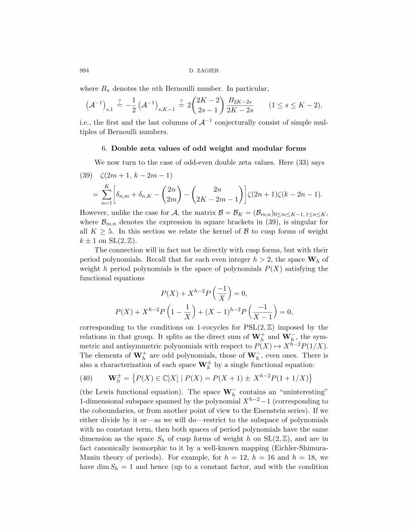
where Bn denotes the nth Bernoulli number. In particular,ÄA−1

äs,1

?= −1

2

ÄA−1

äs,K−1

?= 2

Ç2K − 2

2s− 1

åB2K−2s2K − 2s

(1 ≤ s ≤ K − 2),

i.e., the first and the last columns of A−1 conjecturally consist of simple mul-

tiples of Bernoulli numbers.

6. Double zeta values of odd weight and modular forms

We now turn to the case of odd-even double zeta values. Here (33) says

ζ(2m+ 1, k − 2m− 1)(39)

=K∑n=1

ñδn,m + δn,K −

Ç2n

2m

å−Ç

2n

2K − 2m− 1

åôζ(2n+ 1)ζ(k − 2n− 1).

However, unlike the case for A, the matrix B = BK = (Bm,n)0≤m≤K−1, 1≤n≤K ,

where Bm,n denotes the expression in square brackets in (39), is singular for

all K ≥ 5. In this section we relate the kernel of B to cusp forms of weight

k ± 1 on SL(2,Z).

The connection will in fact not be directly with cusp forms, but with their

period polynomials. Recall that for each even integer h > 2, the space Wh of

weight h period polynomials is the space of polynomials P (X) satisfying the

functional equations

P (X) +Xh−2P

Å−1

X

ã= 0,

P (X) +Xh−2P

Å1− 1

X

ã+ (X − 1)h−2P

Å −1

X − 1

ã= 0,

corresponding to the conditions on 1-cocycles for PSL(2,Z) imposed by the

relations in that group. It splits as the direct sum of W+h and W−

h , the sym-

metric and antisymmetric polynomials with respect to P (X) 7→ Xh−2P (1/X).

The elements of W+h are odd polynomials, those of W−

h , even ones. There is

also a characterization of each space W±h by a single functional equation:

(40) W±h =

¶P (X) ∈ C[X] | P (X) = P (X + 1)± Xh−2P (1 + 1/X)

©(the Lewis functional equation). The space W−

h contains an “uninteresting”

1-dimensional subspace spanned by the polynomial Xh−2−1 (corresponding to

the coboundaries, or from another point of view to the Eisenstein series). If we

either divide by it or—as we will do—restrict to the subspace of polynomials

with no constant term, then both spaces of period polynomials have the same

dimension as the space Sh of cusp forms of weight h on SL(2,Z), and are in

fact canonically isomorphic to it by a well-known mapping (Eichler-Shimura-

Manin theory of periods). For example, for h = 12, h = 16 and h = 18, we

have dimSh = 1 and hence (up to a constant factor, and with the condition

EVALUATION OF THE MULTIPLE ZETA VALUES ζ(2, . . . , 2, 3, 2, . . . , 2) 995

P (0) = 0) precisely one symmetric and one antisymmetric period polynomial,

as follows:

s12(x) = 4X9 − 25X7 + 42X5 − 25X3 + 4X,

s16(x) = 36X13 − 245X11 + 539X9 − 660X7 + 539X5 − 245X3 + 36X,

s18(x) = 24X15 − 154X13 + 273X11

− 143X9 − 143X7 + 273X5 − 154X3 + 24X,

a12(x) = X8 − 3X6 + 3X4 −X2,

a16(x) = 2X12 − 7X10 + 11X8 − 11X6 + 7X4 − 2X2,

a18(x) = 8X14 − 25X12 + 26X10 − 26X6 + 25X4 − 8X2.

On the other hand, the kernels of the matrix BK for K = 5, 6, 7 and 8

are given by

C ·

4

−9

6

−1

0

, C ·

4

−25

42

−25

4

0

, C ·

12

−35

44

−33

14

−2

0

, C ·

36

−245

539

−660

539

−245

36

0

⊕

C ·

56

−150

130

0

−78

50

−8

0

−11pt

,

where in the last case the basis of the 2-dimensional kernel has been chosen to

make the structure more transparent. We see that the kernels for K = 6 and

K = 8 contain vectors whose entries (apart from the final 0) are symmetric

and that these entries coincide with the coefficients of the symmetric period

polynomial s2K(X), while the remaining vectors in the kernel for K = 5, 7 and

8 have entries equal (up to a factor 1/2) to the coefficients of the derivatives

of the antisymmetric period polynomials a2K+2(X):

a′12(x)/2 = 4X7 − 9X5 + 6X3 −X,

a′16(x)/2 = 12X11 − 35X9 + 44X7 − 33X5 + 14X3 − 2X,

a′18(x)/2 = 56X13 − 150X11 + 130X9 − 78X5 + 50X3 − 8X.

The proof that these relations hold, i.e., that there is an injective mapping

(41) W+2K

⊕W−

2K+2 −→ Ker(BK)

as just described, is not too difficult, but I have not been able to show that

this map is an isomorphism, i.e., that there are no other relations. (And in any

case this statement would not permit one to replace “[(K−5)/3] relations” by

“precisely [(K − 5)/3] relations” in Theorem 3, since the linear independence

996 D. ZAGIER

over Q of the numbers ζ(2s + 1)/π2s+1 is not known.) We indicate the proof

briefly.

The first step is to show that all elements in the kernel have last component

equal to 0 (as one can see in the examples given above). This is of interest

since it is equivalent to the statement that there is a vector λ = (λ0, . . . , λK−1)

whose image under Bt is the vector (0, . . . , 0, 1), and that in turn implies an

explicit formula ζ(k) = −2∑K−1m=0 λmζ(2m + 1, k − 2m) for odd zeta values in

terms of odd-even double zeta values. We content ourselves here with giving

the formula for λ, leaving the routine verification of its defining property to

the reader:

λm =1

3(K − 1)·

2 (2K − 1) if m = 0,

2K − 4m− 1 if 1 ≤ m ≤ K − 2,

−(2K − 1) if m = K − 1.

We then observe that the statement that c = (c1, . . . , cK−1, 0)t is in the kernel

of B is equivalent to the statement that the polynomial C(X) :=∑K−1n=1 cnX

2n

satisfies the functional equation

(42) C(X)− C(X + 1)−X2K−1C(1 + 1/X) = (odd polynomial in X).

(This is a direct consequence of the definition of the coefficients of B in (39),

in which the “δn,K” term can now be omitted since we know that cK = 0.) If

we denote by CK the space of even polynomials satisfying (42), then the map

W+2K ⊕W−

2K+2 → CK whose existence and injectivity we want to prove sends

a polynomial P ∈W+2K to C(X) = XP (X) and a polynomial P ∈W−

2K+2 to

C(X) = X2K−1P ′(1/X). (The injectivity of each of these maps separately is

then obvious, and their combined injectivity almost equally so, since the images

have incompatible symmetry properties cn = cK−n and ncn = −(K − n)cK−n.

Note also that CK has an uninteresting 1-dimensional subspace, consisting of

constants, that we are not allowing, but which corresponds under the map just

given to the uninteresting subspace 〈X2K − 1〉 of W−2K+2 that we excluded by

our normalization condition.) Denote the left-hand side of (42) by L. Then if

C(X) = XP (X) with P ∈W+2K , we find

L = (X+1)îP (X)−P (X+1)−X2K−2P (1+1/X)

ó−P (X) = −P (X) = (odd)

by virtue of (40), and if C(X)=X2K−1P ′(1/X) with P ∈W−2K+2, then using

(40) and the symmetry properties P (X)=P (−X) = −X2KP (1/X), we find

L = (X + 1)2K+1 d

dx

ñP

Å −1

X + 1

ã− P

ÅX

X + 1

ã+(X + 1)−2KP (−X)

ô− P ′(X) = −P ′(X),

which is again odd. This concludes the proof of Theorem 3.

EVALUATION OF THE MULTIPLE ZETA VALUES ζ(2, . . . , 2, 3, 2, . . . , 2) 997

It is perhaps worth remarking that we have given a simple description of

the kernel of BK , but not of the relations among the odd-even double zeta

values themselves, which correspond to the kernel of the transpose; e.g., the

kernel of Bt5 is generated by (−6, 17, 13,−27, 3) and we have −6 ζ(1, 10) +

17 ζ(3, 8) + 13 ζ(5, 6) − 27 ζ(7, 4) + 3 ζ(9, 2) = 0. I was not able to find an

explicit description of the elements of the kernel of BtK .

7. Multiple zeta-star values and Hoffman star elements

The “multiple zeta-star values” ζ∗(k1, . . . , kn) are defined (again for ki≥ 1,

kn ≥ 2) by

ζ∗(k1, . . . , kn) =∑

1≤m1≤···≤mn

1

mk11 · · ·m

knn

.

They span the same Q-vector space as the usual MZV’s and one again has the

conjecture that the “Hoffman star elements”

H∗(a0, . . . , ar) := ζ∗(2, . . . , 2︸ ︷︷ ︸a0

, 3, 2, . . . , 2︸ ︷︷ ︸a1

, . . . , 3, 2, . . . , 2︸ ︷︷ ︸ar

) (a0 . . . , ar ≥ 0)

form a Q-basis of this space. The simple Hoffman star elements are given by

the formula

(43) H∗(n) := ζ∗(2, . . . , 2︸ ︷︷ ︸n

) = 2 (1− 21−2n) ζ(2n) (n ≥ 0),

as one sees immediately from the generating function

(44)∞∑n=0

H∗(n)x2n =∞∏m=1

1

1− x2/m2=

πx

sinπx.

The double Hoffman star elements were studied in a recent preprint of Ihara,

Kajikawa, Ohno and Okuda [8], who showed that odd zeta values can be

expressed very simply as rational linear combinations of them. In this section

we give a closed formula for the double Hoffman star elements and a new proof

of this identity.

Recall that Theorem 1 gave the formula

H(a, b) = 2K∑r=1

(−1)rñÇ

2r

2a+ 2

å−Å

1− 1

22r

ãÇ2r

2b+ 1

åôH(K − r) ζ(2r + 1)

for the usual double Hoffman elements, where a, b ≥ 0 and K = a+ b+ 1. The

formula in the star case is very similar.

Theorem 4. For a, b ≥ 0, we have

(45)

H∗(a, b) = −2K∑r=1

ñÇ2r

2a

å− δr,a −

Å1− 1

22r

ãÇ2r

2b+ 1

åôH∗(K − r) ζ(2r + 1),

where K = a+ b+ 1 and H∗(n) is given by (43).

998 D. ZAGIER

Corollary (Theorem 2 of [8]). For K ≥ 1, we have

(46) 2K(1− 2−2K) ζ(2K + 1) =K−1∑a=0

Å1 +

1

2δa,0

ãH∗(a,K − 1− a).

Proof. Just as in the simple Hoffman star case (44), we work with gener-

ating functions. We have∑a, b≥0

H∗(a, b)x2a y2b =∞∑m=1

Ç m∏k=1

1

1− x2/k2

å· 1

m3·Ç ∞∏l=m

1

1− y2/l2

å=

πx

sinπx· πy

sinπy·∞∑m=1

∞∏k=m+1

Ç1− x2

k2

å· 1

m3·m−1∏l=1

Ç1− y2

l2

å=

πx

sinπx· πy

sinπy· −F (y, x)

xy2,

where the last equality comes from equation (11). Now by formula (13) and

the equality F = “F , together with the generating function (44), the right-hand

side of this expression can be rewritten as

− πy

sinπy· A(y + x) +A(y − x)− 2A(x)

y2+

πx

sinπx· B(y + x)−B(y − x)

xy

= −∞∑n=0

H∗(n) y2n ·∞∑r=1

ζ(2r + 1)(x+ y)2r + (x− y)2r − 2x2r

y2

+∞∑n=0

H∗(n) y2n ·∞∑r=1

(1− 2−2r)ζ(2r + 1)(x+ y)2r − (x− y)2r

xy,

and equation (45) follows by comparing coefficients on both sides. The corol-

lary is an immediate consequence, since for 1 ≤ r ≤ K, we have

− 2∑

a+b=K−1

Å1 +

1

2δr,a

ãñÇ2r

2a

å− δr,a −

Å1− 1

22r

ãÇ2r

2b+ 1

åô= − (22r − 1) + 2

Ä1− 2−2r

äÇ22r +

1

2

Ç2r

2K − 1

åå= 2K

Ä1− 2−2K

äδr,K . �

Remarks 1. The simplicity of (46) as opposed to the corresponding formula

for ζ(2K+1) in terms of the original Hoffman elements H(a, b) might give some

hope that the Hoffman star elements are perhaps closer to being a Z-basis of

the Z-lattice of MZV’s. But in fact this is not the case: if one inverts the

matrix occurring in (45) to write the products H∗(n) ζ(2r + 1) as rational

linear combinations of the numbers H∗(a, b), then except in the case n = 0

one again finds large primes in the denominators and no apparent pattern in

the numerators. Nevertheless, the numbers are not completely random. For

EVALUATION OF THE MULTIPLE ZETA VALUES ζ(2, . . . , 2, 3, 2, . . . , 2) 999

instance, for 2 ≤ K ≤ 40 the determinant of the matrix in question is always

divisible by the numerator of B2K+2/(2K + 2) and also by (22K − 1)[K/6]+1.

The former observation is related to similar experimental findings of Masanobu

Kaneko that he communicated to me privately.

2. The proof we have given of Theorem 4 and its corollary is analytic and

works only for the multiple zeta-star values as real numbers, whereas the proof

of Theorem 2 in [8] is algebraic and deduces the identity in question only from

the double shuffle relations. If that proof can be extended to give a similarly

algebraic proof of Theorem 4, then one also gets a new and purely algebraic

proof of Theorem 1 (since the relationship between the generating functions

of H(a, b) and H∗(a, b) can be used in either direction). This would be of

especial interest because for the application to periods of mixed Tate motives

in [2], Brown needs the truth of (7) in the context of motivic zeta values, not

merely of real ones, and has to carry out a subtle inductive argument in order

to deduce this statement from the statement over R.

References

[1] F. Brown, On the decomposition of motivic multiple zeta values. arXiv 1102.

1310v2.

[2] , Mixed Tate motives over ζ, Ann. of Math. 175 (2012), 949–976. http:

//dx.doi.org/10.4007/annals.2012.175.2.10.

[3] P. Deligne and A. B. Goncharov, Groupes fondamentaux motiviques de Tate

mixte, Ann. Sci. Ecole Norm. Sup. 38 (2005), 1–56. MR 2136480. Zbl 1084.

14024. http://dx.doi.org/10.1016/j.ansens.2004.11.001.

[4] L. Euler, Meditationes circa singulare serierum genus, Novi Comm. Acad. Sci.

Petropol. 20 (1776), 140–186, Opera Omnia, Ser. I, vol. 15, B.G. Teubner, Berlin

(1927), 217–267. Available at http://eulerarchive.maa.org/pages/E477.html.

[5] H. Gangl, M. Kaneko, and D. Zagier, Double zeta values and modular

forms, in Automorphic Forms and Zeta Functions, World Sci. Publ., Hacken-

sack, NJ, 2006, pp. 71–106. MR 2208210. Zbl 1122.11057. http://dx.doi.org/10.

1142/9789812774415 0004.

[6] A. B. Goncharov, Galois symmetries of fundamental groupoids and non-

commutative geometry, Duke Math. J. 128 (2005), 209–284. MR 2140264.

Zbl 1095.11036. http://dx.doi.org/10.1215/S0012-7094-04-12822-2.

[7] M. E. Hoffman, The algebra of multiple harmonic series, J. Algebra 194

(1997), 477–495. MR 1467164. Zbl 0881.11067. http://dx.doi.org/10.1006/jabr.

1997.7127.

[8] K. Ihara, J. Kajikawa, Y. Ohno, and J. Okuda, Multiple zeta values

vs. multiple zeta-star values, J. Algebra 332 (2011), 187–208. MR 2774684.

Zbl 05969524. http://dx.doi.org/doi:10.1016/j.jalgebra.2010.12.029.

1000 D. ZAGIER

[9] Y. Ohno and D. Zagier, Multiple zeta values of fixed weight, depth, and height,

Indag. Math. 12 (2001), 483–487. MR 1908876. Zbl 1031.11053. http://dx.doi.

org/10.1016/S0019-3577(01)80037-9.

[10] T. Terasoma, Mixed Tate motives and multiple zeta values, Invent. Math.

149 (2002), 339–369. MR 1918675. Zbl 1042.11043. http://dx.doi.org/10.1007/

s002220200218.

(Received: March 3, 2011)

Max Planck Institute for Mathematics, Bonn, Germany

E-mail : don.zagier@mpim-bonn.mpg.de