1

Evaluation of the HOMME Dynamical Core in the Aqua-Planet Configuration

of NCAR CAM4: Rainfall

Saroj K. Mishra1, 2, Mark A. Taylor3, Ramachandran D. Nair2, Peter H. Lauritzen2, Henry

M. Tufo1, 2, Joseph J. Tribbia2

1Department of Computer Science, University of Colorado, Boulder, CO, USA

2National Center for Atmospheric Research (NCAR), Boulder, CO, USA

3Sandia National Laboratories, Albuquerque, NM, USA

Submitted to Journal of Climate: May-11-2010

Revised for Journal of Climate: December-15-2010

Corresponding Address: saroj@ucar.edu

Institute for Mathematics Applied to Geosciences (IMAGe)

#National Center for Atmospheric Research (NCAR)

Boulder, CO, 80305, USA.

Phone: 303-497-2486

Fax: 303-497-2483

#The National Center for Atmospheric Research is sponsored by the National Science Foundation

2

Abstract

The NCAR-Community Climate System Model version 4 (CCSM4) includes a new

dynamical core option based on NCAR’s High-Order Method Modeling Environment

(HOMME). HOMME is a petascale capable high-order element-based conservative

dynamical core developed on the cubed-sphere grid. Initial simulations have been

completed in aqua-planet configuration of CAM4, the atmospheric component of CCSM4.

We examined the results of this simulation and assessed its fidelity in simulating rainfall,

which is one of the most important components of the Earth’s climate system. For this we

compared the results from two other dynamical cores of CAM4, the finite volume (FV) and

Eulerian (EUL).

Instantaneous features of rainfall in HOMME are similar to FV and EUL. Similar to

EUL and FV, HOMME simulates a single peak Inter Tropical Convergence Zone (ITCZ)

over the equator. The strength of the ITCZ is found to be almost same in HOMME and

EUL but more than that in FV. It is observed that in HOMME and EUL there is higher

surface evaporation, which supplies more amount of moisture into the deep tropics and

gives more rainfall over the ITCZ. The altitude of maximum precipitation is found to be at

almost the same level in all the three dynamical cores. The eastward propagation of rainfall

bands is organized in FV and HOMME, and more prominent than in EUL. The phase speed

of the eastward propagation in HOMME is found to be higher than that in FV. Our results

show that, in general, the rainfall simulated by HOMME falls in a regime between that of

FV and EUL. Hence, we conclude that the key aspects of rainfall simulation with HOMME

falls in an acceptable range, as compared to the existing dynamical cores used in the model.

3

1 Introduction

General circulation models (GCMs) are an effective tool to improve our

understanding of the present and past climate as well to predict the future climate. The

present day numerical models are yet to capitalize on the enormous computing power made

available by petascale capable high performance computers. The GCMs broadly consist of

two components, namely, the dynamical core and the physical parameterization suite. The

dynamical core numerically solves the system of partial differential equations, which

govern the fluid motion, while the physics package provides the numerous forcing terms

used in these equations.

In order to take advantage of the high performance computing, improvement of the

dynamical core used in the present day GCM is of paramount importance. Currently, most

of the operational dynamical cores use latitude-longitude based grids. The grid lines cluster

at the pole, creating a potentially severe CFL restriction on the time step. There are many

successful techniques to handle this pole problem; however, most of them (e.g., polar

filters) substantially degrade parallel scalability by limiting the model to one-dimensional

domain decomposition strategies. However, future evolution of the Community Climate

System Model (CCSM) into an Earth system model requires a highly scalable and accurate

formulation of the dynamics of the atmosphere.

The High Order Method Modeling Environment (HOMME) is a highly scalable,

global hydrostatic atmospheric modeling framework (Dennis et al., 2005; Nair 2007; Nair

2009). Recently, HOMME has been integrated into the Community Atmospheric Model

(CAM), the atmospheric component of the CCSM. HOMME relies on a cubed-sphere grid,

where the planet Earth is tiled with quasi-uniform quadrilateral elements, free from polar

singularities. HOMME is the first dynamical core ever that allows for full two-dimensional

4

domain decomposition in CAM.

Recent performance comparisons of CAM-FV and CAM-HOMME (A. Mirin,

personal communication, 2010) show that at the resolution used here, CAM-FV is twice as

fast as CAM-HOMME on 32 processor cores of the JaguarPF Cray XT-5 at Oak Ridge

National Laboratory. Due to CAM-HOMME's increased scalability, CAM-HOMME starts

to outperform CAM-FV on 512 cores and higher. CAM-HOMME achieves a maximum

integration rate of 82 simulated-years-per-day (SYPD) on 2700 cores, compared to CAM-

FV's maximum of 50 SYPD on 3328 cores. At higher resolutions, the improvements due to

increased scalability become larger. At 1/4 degree resolution, on the Intrpid BG/P system

at Argonne National Laboratory, CAM-HOMME can achieve 12 SYPD on 86,400 cores,

while CAM-FV achieves its maximum rate of 2.5 SYPD on 53248 cores (Edwards et al.,

2011)

HOMME simulations presented in this paper use the physics package of CAM,

version 4 (Neale et al., 2010) in the aqua-planet configuration. Since rainfall is one of the

most important components of the Earth's climate system, its simulation is examined in this

paper. Here the simulated rainfall from HOMME has been compared with FV and EUL

dynamical cores.

The organization of the paper is as follows. Section 2 briefly outlines model details

and section 3 describes the simulation details. Results are presented in section 4, followed

by the summary and conclusions in section 5.

2 Brief Description of CAM4

The Community Atmosphere Model version 4 (CAM4) is the sixth generation of

atmospheric general circulation models (AGCMs) developed by the atmospheric modeling

5

community in collaboration with the National Center for Atmospheric Research (NCAR).

The source code, documentation and input datasets for the model are freely available from

the CAM website (http://www.ccsm.ucar.edu/models/ccsm4.0/cam/). Since a detail

description of CAM4 is given in Neale et al. (2010), we will not discuss the details of

model here. Nevertheless, certain aspects of the model, relevant to this work, are explained

in the following.

CAM4 has been designed to produce simulations with reasonable accuracy for

various dynamical cores and horizontal resolutions. For this study, FV, EUL, and HOMME

dynamical cores were used at 10 equivalent resolutions in horizontal and 26 levels in the

vertical. The model uses the hybrid vertical coordinate, which is terrain following at earth's

surface, but reduces to pressure coordinate at higher levels near the tropopause.

(a) CAM4 Physics

All the three dynamical cores use the same physical parameterization package,

consisting of moist precipitation processes, clouds and radiation processes, surface

processes, and turbulent mixing processes. Each of these in turn is subdivided into various

components. The moist precipitation processes consist of the deep convective, shallow

convective and stratiform components. The deep convective processes are parameterized by

the revised version of the Zhang-McFarlane convection scheme, in which the calculation of

CAPE has been modified to include the effect of entrainment dilution (Neale et al., 2008).

In addition, in the revised version, convective momentum transport parameterized by

Gregory et al. (1997) has been included (Richter and Rasch, 2008). The shallow convective

process is parameterized by Hack (1994). The parameterization of the stratiform processes

in CAM4 is described in Rasch and Kristjansson, (1998) and Zhang et al. (2003). In the

6

default configuration of the model, the parameterizations are applied over a time interval of

1200 s for EUL, 1800 s for FV, and 1800 s for HOMME.

(b) CAM4 Dynamical cores

The EUL dynamical core is a three-time-level, spectral transform applied at T85

truncation on a 256X128 quadratic grid. Moisture transport in EUL is done using a

monotonic semi-Lagrangian method, which is time split in the horizontal and vertical

directions. The trajectory calculation used for moisture transport uses a quasi-cubic

interpolation. A detailed scientific documentation of the EUL dynamical core is given in

the CAM3 scientific documentation (Neale et al. 2010).

CAM FV integrates the quasi-hydrostatic equations of motion in flux-form. The

horizontal spatial discretization grid is based on a 'CD'-grid approach that involves a half-

time-step update on the Arakawa C grid that provides the time-centered winds to complete

a full time step on the Arakawa D grid (Lin and Rood 1997). In the vertical, a floating

Lagrangian coordinate is used, that is initialized from a standard hybrid-sigma vertical

coordinate (Eulerian grid). The Lagrangian vertical coordinate 'floats' for several

consecutive time-steps (default setup for this study is 4) before a vertical remapping

transfers the prognostic variables back to the Eulerian reference grid. The vertical

remapping procedure is formulated so that it conserves total energy (Lin 2004). The

advantage of the floating Lagrangian coordinate approach is that the equations of motion in

each layer reduce to two-dimensional shallow water equations, hence, only two-

dimensional operators are needed. The two-dimensional advection operator used in CAM-

FV follows the Lin and Rood (1996) scheme. The water variables (specific humidity, cloud

liquid water and ice) and tracers are transported on longer time-steps than that used for the

7

momentum, thermodynamic and continuity equation for air (setup in this study is 4

dynamics time-steps per tracer time-step) using super-cycling (e.g., Lin 2004). The Lin and

Rood (1996) advection scheme applies a combination of Piecewise Constant and Piecewise

Parabolic Methods (Colella and Woodward 1984) in its dimensionally split one-

dimensional operators. The stability properties of this configuration (and others) are

discussed in detail in Lauritzen (2007). The moisture transport in CAM-FV is computed

with the Lin and Rood (1996) transport scheme, which is a flux-form finite-volume

scheme, formulated in terms of one-dimensional operators. The flux-operators are based on

the Piecewise Parabolic Method (PPM, Colella and Woodward, 1984) that are formally

third-order accurate on uniform grids, and hence the implementation on the regular latitude-

longitude grid is formally second order. The damping and dispersion properties of the

scheme are discussed in Lauritzen (2007). Monotonicity is enforced using reconstruction

function filtering in each coordinate direction which prevents negative undershoots in each

coordinate direction. The discretization in CAM FV is such that vorticity modes at the grid

scale are controlled through sub-grid-scale function limiters in the advection operator.

Divergent modes, however, are not controlled at the grid scale through limiters wherefore

explicit second-order divergence damping is applied to the momentum equations. To

stabilize the model in the presence of gravity waves, one-dimensional polar filters are

applied along latitudes. More information on CAM-FV and the performance in idealized

tests can be found in Lauritzen et al. (2010). Diffusion in CAM-FV is through the

monotonicity constraints in the advection operator as well as explicitly added divergence

damping (Neale et. al. 2010).

HOMME uses the continuous Galerkin spectral finite element method (Taylor et al.,

2010), often abbreviated as the spectral element method (SEM). This method is designed

8

for fully unstructured quadrilateral meshes. The current configurations in CAM are based

on the cubed-sphere grid. The main motivation for the inclusion of HOMME is to improve

the scalability of CAM by introducing quasi-uniform grids, which require no polar filters

(Taylor et al., 2008). HOMME is also the first dynamical core in the CAM that locally

conserves energy in addition to mass and two-dimensional potential vorticity (Taylor,

2010). HOMME represents a large change in the horizontal grid as compared to the other

dynamical cores in CAM. Almost all other aspects of HOMME are based on a combination

of well-tested approaches from the Eulerian and FV dynamical cores. For tracer advection,

HOMME is modeled as closely as possible on the FV dynamical core. It uses the same

conservation form of the transport equation and the same vertically Lagrangian

discretization (Lin 2004). The HOMME dynamics are modeled as closely as possible on

Eulerian dynamical core. They share the same vertical coordinate, vertical discretization,

hyper-viscosity based horizontal diffusion, top-of-model dissipation, and solve the same

moist hydrostatic equations. The main differences are that HOMME advects the surface

pressure instead of its logarithm (in order to conserve mass and energy), and HOMME uses

the vector-invariant form of the momentum equation instead of the vorticity-divergence

formulation. The time stepping in HOMME is a form of dynamics/tracer/physics sub-

cycling, achieved through the use of multi-stage 2nd order accurate Runge-Kutta methods.

The tracers and dynamics use the same time step, which is controlled by the maximum

anticipated wind speed, but the dynamics uses more stages than the tracers in order to

maintain stability in the presence of gravity waves.

The moisture transport in CAM-HOMME is computed with the same vertically

Lagrangian approach (Lin 2004) as used in CAM-FV, and the former uses the monotone

vertical remap from (Zerroukat et al, 2005). The transport within the Lagrangian surfaces is

9

done using the locally mass conserving spectral element discretization (Taylor and

Fournier, 2010), combined with a sign-preserving limiter (Taylor et al., 2009). The spectral

element advection operator is 4th order accurate on the cubed-sphere grid with very little

diffusion, so additional scale selective mixing is added via the same hyper-viscosity term

used in the dynamics (Neale et al., 2010). The spatial diffusion used in CAM-HOMME is

modeled on that used in CAM-Eulerian. CAM-HOMME uses the same hyper-viscosity

operator, and the 1-degree results presented here use the same hyper-viscosity coefficient as

T85 CAM-Eulerian. The hyper-viscosity operator is solved explicitly and time-split from

the rest of the dynamics, using a mixed finite element integrated-by-parts formulation

(Neale et al., 2010).

3 Simulation Details

For the examination of the performance of HOMME in NCAR-CAM4, we carried

out a set of simulations with HOMME, FV (the default dynamical core of CAM4), and

EUL. All the simulations were performed in the aqua-planet configuration of CAM4. In

this configuration, all the land points are replaced by ocean points such that the surface drag

coefficients, albedo, and evaporation characteristics are homogeneous over the globe. A

further simplification is obtained by fixing the solar declination to its value on March 21,

which puts the sun overhead at the equator. This produces another desirable simplification

by providing approximate hemispheric symmetry of insolation forcing. The experiments

have been performed with a zonally symmetric SST profile as lower boundary condition.

The distribution of SST used in the simulation is given in equation 1, which is the same as

the control SST used by Neale and Hoskins (2000):

10

27[1 - sin2 (3φ/2)]0C : -π/3 < φ < π/3

TS(λ, φ) = (1)

00 C : Otherwise

where, TS=Sea Surface Temperature ( 0C), λ = longitude, φ = latitude.

The initial condition for all simulations was from a previous aqua-planet simulation.

All the simulations were performed for 24 months, and the last 18 months were considered

for the analysis. The default physics tunings were used for all the simulations. The monthly

and daily model outputs have been analyzed to understand various issues pertaining to the

steady (time mean) and transient (temporally varying) characteristics of simulated climate.

4 Results

(a) Instantaneous Distribution

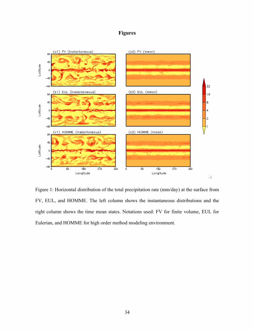
Figure 1 shows the horizontal distribution of the total precipitation at the surface from FV,

EUL, and HOMME. The left column of the figure shows the instantaneous features, and the

right column shows the time mean features. For the study of the instantaneous features,

several snapshots were analyzed and the basic characteristics were found to be similar. One

representative instant has been arbitrarily chosen for illustration. The storm-like zonally

oriented structures in the tropics and baroclinic wave-like meridionally oriented structures

in the mid-latitudes are evident in all the three dynamical cores (see the left column). The

interactions between the tropics and extra-tropics show up prominently in the instantaneous

11

patterns. The time mean features shown in the right column are the average of the

instantaneous features. The inter-tropical convergence zone (ITCZ) appears over the

equator saliently. The dry zones over sub-tropical highs are distinct. The secondary rainfall

zones over mid-latitude storm tracks are also distinctly clear in all the three dynamical

cores. The notable difference is that the ITCZ in EUL and HOMME is comparatively

sharper and more confined to the equator than that in FV. By and large, the horizontal

distribution of rainfall is found to be similar in all the three dynamical cores.

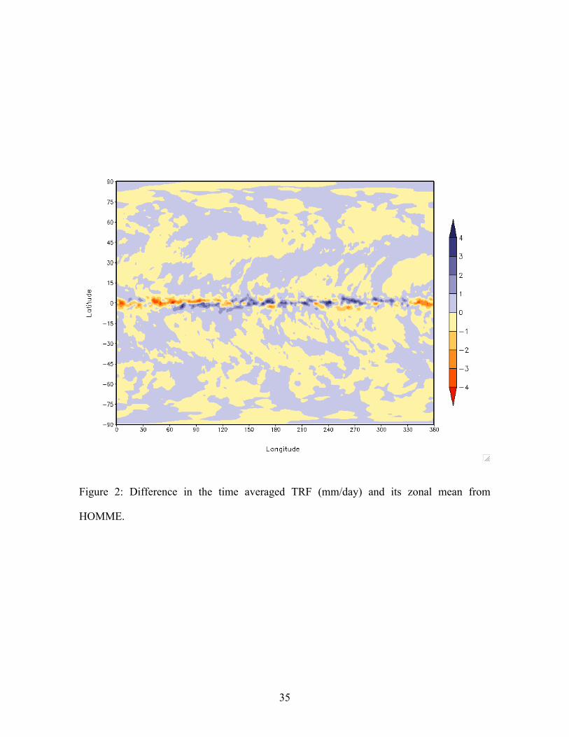
Since the HOMME dynamical core is based on the cubed-sphere grid, it is desirable

to examine the wave-4 signal from the simulations. In figure 2, the difference in the time

averaged precipitation and its zonal mean is shown. However, no signature of the wave-4 is

evident in the plot. This indicates that the simulation is devoid of such noise and the length

of integration is long enough. The other two dynamical cores are based on lat-lon grid and

known to be free from wave-4 noise.

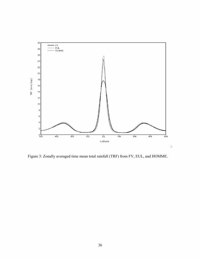
(b) Mean State

In this section we compare the time mean state of precipitation from FV, EUL, and

HOMME. Figure 3 shows the zonally averaged time-mean surface reaching total rainfall

(TRF) for the three dynamical cores. We find that the peak of the ITCZ is over the equator

in all the three cases. The morphology of the ITCZ is found to be similar. However, there is

notable difference in the magnitude of the TRF. Over the equator, the TRF in EUL and

HOMME is higher than that in FV. The mean TRF over the equator in FV is ~18 mm/day,

whereas in EUL & HOMME it is around 25 mm/day. The difference is around 40% of the

mean value of FV. However, there is almost no difference in TRF between EUL &

HOMME. Since TRF constitutes of three components, namely, deep convective rainfall

12

(DRF), shallow convective rainfall (SRF), and large-scale rainfall (LRF), in the following

we analyze them individually.

Figure 4 shows the zonally averaged time mean surface reaching DRF, SRF, and

LRF, for FV, EUL, and HOMME. All the three components are found to be higher in EUL

than that in FV. Among the three components, the difference in DRF between EUL and FV

dominates the other two components. On the contrary, the comparison between FV and

HOMME indicates that DRF is almost same for both of them, whereas the other two

components are higher in HOMME than that in FV. The difference in LRF between

HOMME and FV is nearly double of the difference in SRF. In other words, the higher TRF

in EUL is primarily due to more DRF, whereas in HOMME it is mainly due to more LRF.

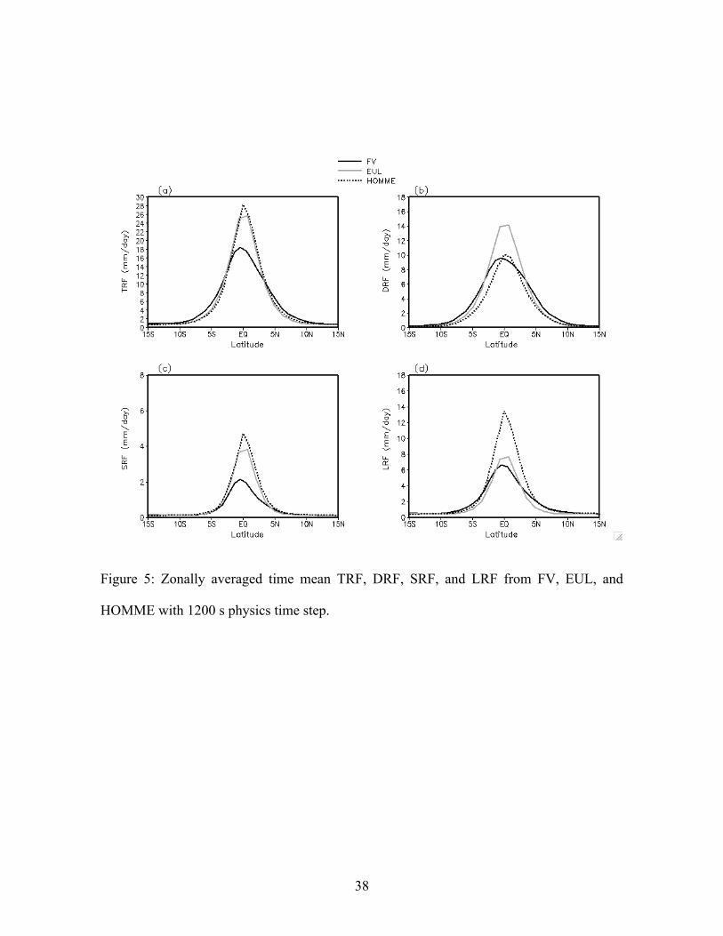
Since rainfall simulation is sensitive to time step (Williamson and Olson, 2003;

Mishra et al., 2008) and is different in the three dynamical cores, we will examine its

contribution to the differences in the there simulations. In order to do so, we carried out two

additional simulations with FV and HOMME with 1200 s. Figure 5 shows the zonally

averaged time mean precipitation from the three simulations. It is noticed that TRF is

largely similar in EUL and HOMME, and more than that in FV. Higher TRF in EUL is

primarily due to more DRF, whereas in HOMME it is mainly due to more LRF. The result

is similar to that seen in the simulations with default time steps. This infers that, the

difference in the simulations with the three dynamical cores is not due to different physics

time steps, rather due to the difference associated with the formulation of the dynamical

cores and their indirect effects through the physics parameterization. However, TRF is

found to be marginally increasing with the reduction of time step, which is due to the

enhancement in LRF. This result is in agreement with Mishra et al. (2008). They showed

that TRF and LRF increase with decrease in time step and the impact is less severe in the

13

smaller time step regime.

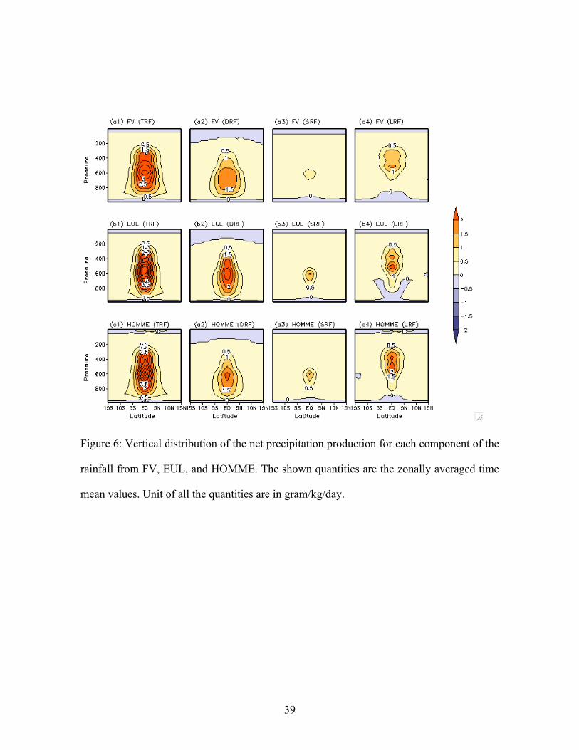
The surface reaching rainfall is the vertical integral of the net precipitation

production at each model level. The net precipitation production at any level is the

condensation minus re-evaporation of precipitation and cloud liquid water at that

corresponding level. In figure 6, the vertical distribution of the net precipitation production

is shown for FV, EUL, and HOMME. The first column shows the vertical distribution of

the TRF production. Similarly, the second, third, and fourth columns show the vertical

distribution of DRF, SRF, and LRF respectively. The figure shows that in all three cases

the net TRF production is vertically extended over the entire troposphere, except for a few

near-surface and top of the model layers. The latitudinal extent and vertical distribution of

TRF looks alike in the three dynamical cores. The altitude of peak TRF occurs around the

same level. However, there is a notable difference in their magnitudes i.e., TRF in EUL and

HOMME is more than that in FV, which is in agreement with the preceding discussion. In

all the three cases, DRF occurs in the lower and mid troposphere, accompanied by re-

evaporation of precipitation and cloud liquid water in the upper troposphere. The third

column shows that there is very little SRF in FV, as compared to that found in EUL and

HOMME. In all the three dynamical cores the SRF production occurs in the mid and lower

troposphere with peaks at around 600 hPa. From the fourth column it can be seen that LRF

occurs in the middle and upper troposphere. The peak of the LRF occurs at around 500 hPa

in all the three cases. There is considerable amount of re-evaporation of LRF seen in the

lower troposphere and near-surface layers. Overall, the vertical distribution of precipitation

production is similar in the three dynamical cores.

In figure 6, it is seen that most of the precipitation occurs within the latitudinal belt

of 5S to 5N. In order to make a closer comparison between the vertical profiles of

14

precipitation, we have shown the area averaged (0E-360E, 5S-5N) time-mean precipitation

production rate for FV, EUL, and HOMME in figure 7. The figure shows a close

resemblance in their profiles. The peak of the precipitation production occurs at around 600

hPa in all three cases. Near the surface (below 950 hPa), the net precipitation production is

negative, which is due to the fact that the re-evaporation of falling precipitation is more in

these layers. The notable point here is that there is a systematic difference in the magnitude

of the precipitation production in the mid troposphere between the three cases. EUL has the

largest precipitation production, whereas FV has the smallest, and HOMME falls in

between these two.

In order to get an overall idea about the global mean values, we analyzed these

quantities for the three dynamical cores. Table 1 shows the global mean TRF from FV,

EUL, and HOMME. The values are very close to each other, i.e., difference among them is

on the order of 2.5% of their mean values. Secondly, the global mean value for HOMME

falls in between that of the other two dynamical cores.

(c) Intensity and Frequency

Here we show the intensity and frequency of rainfall for FV, EUL, and HOMME.

For this we analyzed the daily rainfall data. Since in the preceding section we noticed that

the region of significant difference is the deep tropics (0E-360E, 10S-10N), we will focus

primarily on this region. Figure 8 shows the frequency distribution of daily rainfall rates

(left panel) and the total rainfall falling in each bin (right panel). The rainfall rates are

categorized into four categories, based on the intensity of rain rate, namely, dry, light,

moderate, and heavy categories. Vertical lines in figure 8 indicate these categories. Figure

8a shows that the frequencies in the dry and heavy categories are higher in EUL and

15

HOMME than in FV. In the light and moderate categories the reverse is true. Although the

frequencies in the dry category are higher, when the frequencies were multiplied with the

respective rainfall rates (accumulated rainfall), they become almost equal in the three

dynamical cores (see figure 8b). Secondly, the accumulated rainfall in the light and

moderate categories are highest in FV, than in HOMME, and least in EUL. Whereas the

rainfall accumulated in the heavy category is found to be higher in EUL and HOMME than

that in FV. Hence, the higher amount of TRF in HOMME and EUL comes from the heavy

rainfall category. There appears a mismatch between figures 8a and 8b, which is counter-

intuitive, but this is because of the fact that within the categorized bin, there is an internal

shift. For example, in heavy category, the frequency in EUL is higher than that in FV,

whereas the accumulated rainfall in heavy category shows the reverse. We investigated by

making finer bin size in this category and noticed that there was an internal shift towards

the upper end in HOMME, i.e., there are more number of points with higher rainfall rates

than that in EUL in the deep tropics.

(d) Time-Longitude Realization

The time mean features for FV, EUL, and HOME have been discussed in the

previous section. Since the transients play a cumulative role in forming the time mean

steady state, here we discuss the transient activities. In section 5-b we saw that the

difference between the dynamical cores was mainly found in the equatorial belt, where

most of the transient activities constitute the zonally propagating waves. Hence, we will

consider this region and discuss the zonal propagation characteristics via time-longitude

diagrams.

Figure 9 shows the time-longitude diagrams of rainfall over the equator (2.S to

16

2.5N) for 180 days. Daily data has been plotted in the figure. All of them (FV, EUL, and

HOMME) show the eastward propagation. This resembles observed equatorial Kelvin

waves (Wheeler and Kiladis 1999). These rainfall bands appear to move over a range of

speeds and wave numbers, however there are distinct differences between the three cases.

In FV, eastward propagating organized rainfall bands appear. They propagate 3600

in 30 to 40 days. While in EUL, the rainfall appears in patches in a discrete manner. The

rainfall bands are not well organized. In HOMME, streaks of well-organized rainfall are

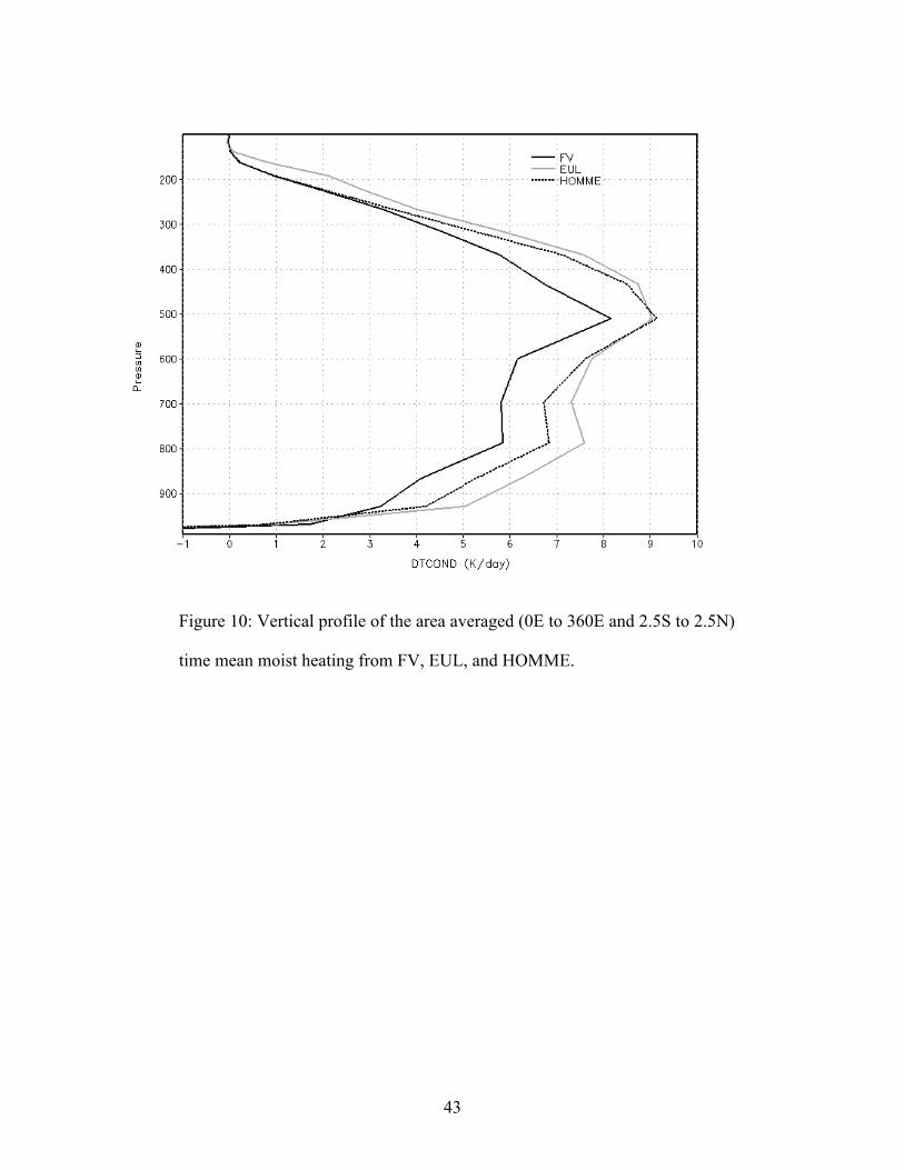
noticed. They propagate 3600 in 20 to 30 days. Since vertical structure of the moist heating

is crucial in determining the speed of the eastward propagations, we have shown the same

for the three dynamical cores in figure 10. The figure shows that the profiles are largely

similar. All of them have most of their heating in the upper troposphere and have top-heavy

heating structure. Comparison of FV and EUL indicates that throughout the troposphere,

EUL has more heating rate than FV. The heating profile of HOMME largely falls in

between the other two dynamical cores in the lower troposphere. However around 500 hPa,

the heating in HOMME is closer to EUL and significantly more than that in FV. Hence, the

top-heaviness in the heating profile is more in HOMME than FV. This is associated with

the faster phase speed of the eastward propagation in HOMME.

(e) Associated Variables

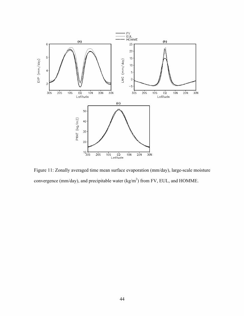
In figure 11, the meridional variation of surface evaporation (EVP), large-

scale moisture convergence (LMC) and vertically integrated precipitable water

(PWAT) is shown for FV, EUL, and HOMME. Figure 11-a shows that EVP is highest for

EUL, lowest for FV and intermediate for HOMME. Over the equatorial belt, LMC in EUL

and HOMME are nearly same and more than that in FV (see figure 11-b). Local

17

evaporation and large-scale moisture convergence are the two sources of moisture for

rainfall production. Comparison of the scales of the figure 11-a and 11-b indicates that

LMC is the primary source of moisture leading to higher rainfall over the ITCZ in EUL and

HOMME than in FV. PWAT is found to be almost same in all the three dynamical cores,

except over the equator, where EUL has marginally more than that in FV and HOMME.

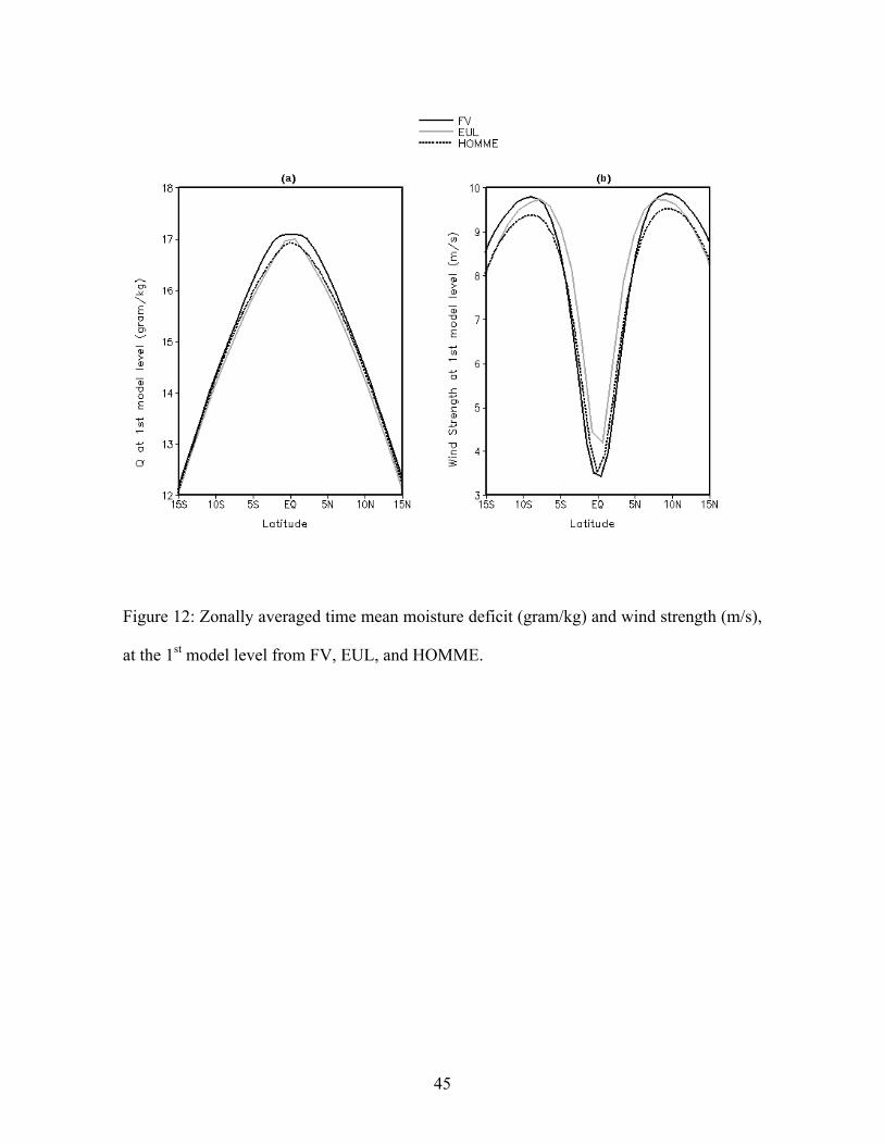
In CAM4, the surface evaporation is computed as shown below (Neale et al., 2010):

EVP = ρA |ΔV| CE dQ (2)

where, ρA is the atmospheric surface density, and ΔV and dQ are the wind strength and

moisture deficit at the lowest model level, respectively. Figure 12-a shows that moisture

(Q) at the 1st model level is almost same in EUL and HOMME and lower than that in FV.

In other words, dQ in EUL and HOMME is higher than that in FV. Figure 12-b shows that

wind strength at the lowest level of the model is higher in EUL than in HOMME and FV

over the equatorial belt. However beyond 5S/N the wind strength in EUL and HOMME is

lesser than that in FV. Hence, the higher evaporation in EUL over the equatorial belt is

attributed partly to higher dQ and partly to the higher wind speed than that in FV. Beyond

5S/N the higher evaporation is solely due to the higher moisture deficit, since the wind

speed therein is lesser than FV. However, the higher EVP in HOMME over the equatorial

belt is primarily due to the higher moisture deficit, since the wind speed therein is almost

same as FV.

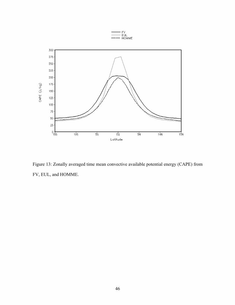
Figure 13 shows the convective available potential energy (CAPE) for FV, EUL,

and HOMME. It is seen that over the equatorial belt, EUL has significantly higher CAPE

than FV and HOMME, which is around 135% of the mean CAPE in FV. This is the reason

18

for the higher amount of deep convective rainfall in EUL. However, there is no such

significant difference in CAPE between FV and HOMME, leading to similar magnitudes of

DRF.

The vertical profiles of area averaged (0E-360E, 5S-5N) time mean relative

humidity (RH), specific humidity (Q), and temperature (T) are compared in figure 14. RH

is found to be lesser (by around 3%) in HOMME than FV, over the whole troposphere

except at 900 hPa. On the contrary, RH in EUL is found to be higher (by around 4%) in

most of the layers, except those adjacent to the surface and between 900-700 hPa, where

the reverse is true. Figures 14-b and 14-c show the corresponding specific humidity and

temperature differences. It is seen that, in the middle and lower troposphere, the profile of

the difference in specific humidity resembles very closely to that of the difference in RH,

which is further supported by the observed temperature profiles (see figure 14-c). In the

upper troposphere, the lesser RH in HOMME and higher RH in EUL are mainly because of

the higher temperature in HOMME and lower temperature in EUL, respectively, since the

difference in Q in these altitudes is almost negligible. Moisture in the boundary layer but

above the surface layer (around 900 hPa) is greater in EUL than that in FV and HOMME,

which seems to be associated with the higher CAPE in EUL.

(f) General Circulation Diagnostics

Generally the largest spatial variation of atmospheric quantities occurs in the

vertical and meridional directions, so analysis of the lat-height cross-section of zonal mean

quantities is a useful exercise and provides an insight into the general circulation of the

atmosphere. For this we analyzed temperatures, zonal wind, vertical velocity, and specific

humidity from the three dynamical cores.

19

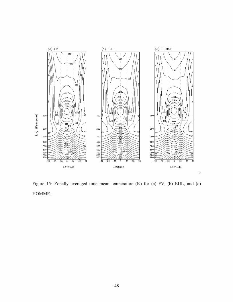
In figure 15, zonal mean temperatures are shown from FV, EUL, and HOMME. In

general, the similarity between the three distributions is remarkable. The pole-to-equator

temperature difference is about 300 C at the earth’s surface. The latitudinal temperature

gradient is identical in all of them. In the lower stratosphere the temperatures increase by

about 250 C from the equator to mid-latitudes, but decrease again with a further increase in

latitudes. The magnitude and altitude of the tropopause temperatures is similar in all of

them. The pole-to-equator difference of the height of the tropopause in the model is similar

in all the three dynamical cores. In high latitudes a stable layer appears primarily due to the

stabilizing effects of baroclinic waves and poleward advection of heat by the large scale

eddies. In the upper stratosphere, the decrease of temperatures from equator to pole is about

250 C. We further examined the vertical profile of temperatures at various latitudes from the

three dynamical cores. The notable difference noticed (not shown here) is, over the

equatorial region the atmosphere is marginally (~ 0.50 C) warmer in HOMME than that in

FV. Between EUL and FV, EUL has a warmer (by ~ 0.50 C) atmosphere in the lower

troposphere and stratosphere, however, a cooler atmosphere in the middle and upper

troposphere. In general, the thermal structure of the model atmosphere looks very similar in

the three dynamical cores.

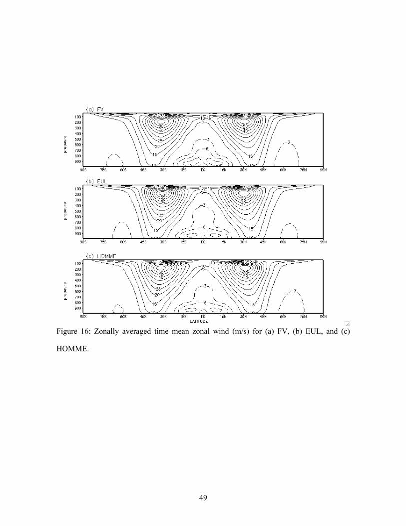
Figure 16 shows the longitudinal mean zonal wind for FV, EUL, and HOMME. The

patterns of the lower tropospheric easterlies and the upper tropospheric westerlies look

similar. Intensity of the jet and its spatial position agree well. It is found that, the regions of

largest latitudinal gradient in temperature (Fig. 15) are coincident with those of the highest

vertical gradient of zonal wind in Fig. 16. This confirms that, the two fields are close to a

state of thermal wind balance. Similarly mean meridional circulation was analyzed from the

three dynamical cores (not shown here). It was noticed that the positions of the ITCZ and

20

positions of the strongest ascent are at the same latitudes, which was anticipated. The

notable differences between the three cases are the following: in EUL the circulation over

the equatorial belt is marginally stronger. The rising limb of the Hadley cell shifts towards

the equator in EUL, associated with strong surface winds over the equatorial belts. This

strengthening of the circulation, in turn, leads to an increase in the moisture convergence

into the equatorial region. However, the zonal and meridional circulation is found to be

largely similar in all of them.

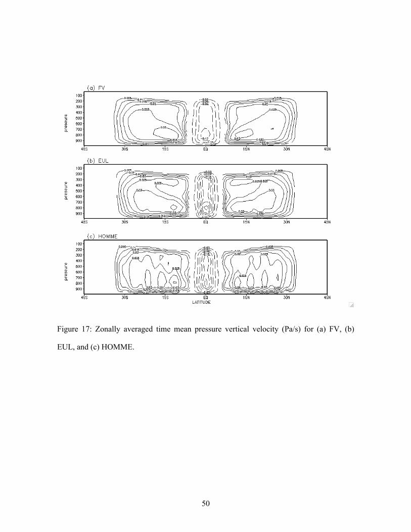
Zonally averaged time-mean vertical pressure velocity (omega) is shown in figure

17, for FV, EUL, and HOMME. A negative value of omega is associated with ascending

motion, which is indicated by the dashed contours. It is observed that, the ascending limb is

more confined to the equator in EUL and HOMME. The latitudinal positions of the

maximum omega are noticed over the corresponding locations of ITCZ, i.e., over the

equator. The altitude of maximum omega occurs in the lower troposphere in all of them.

Notable is the difference in strengths of omega. The strength is largely similar in EUL and

HOMME, but greater than that in FV. Previously, in figure 10 it was seen that, the rate of

moist heating over the equatorial region is higher in EUL and HOMME, which is

associated with the stronger vertical velocity.

Finally, the distribution of specific humidity from the three dynamical cores is

shown in figure 18. The very dry upper troposphere and stratosphere, the wet lower

troposphere, and the dry subtropics are common in all of them. The spatial pattern of

specific humidity and its magnitude are similar. It has a maximum over the surface layer of

the equatorial belt and decreases with increase in altitude and/or latitude. This is associated

with the fact that the primary source of moisture, i.e., surface evaporation occurs in the

lowest model level, which is strongest in the tropics and decreases with increase in

21

latitudes. Furthermore, the moisture sink, i.e., precipitation removes the moisture from the

mid and upper troposphere. Large-scale circulation redistributes the moisture in the

atmosphere, makes it moister in convergence zone (e.g. ITCZ) and makes it drier in the

divergence zone (e.g. subtropical highs). The combined effect of the three factors governs

such a distribution of the moisture in the atmosphere. The vertical and meridional gradient

of the specific humidity is similar in all of them. By and large, the distribution of specific

humidity is similar. However, comparison of the vertical profiles from the three dynamical

cores over individual latitudes showed marginal differences (not shown here). For instance,

over the equatorial belt, the surface layer is comparatively more moist in FV, but in the

lower troposphere (around 900 hPa) the reverse is true. However, in the upper troposphere,

EUL is found to have the highest specific humidity, followed by FV, and HOMME,

respectively.

5 Summary and Conclusions

The High Order Method Modeling Environment (HOMME) is a new spectral

element-based dynamical core included in the CCSM4. HOMME is a highly scalable

dynamical core that achieves the conservation of mass, potential vorticity (in 2D), and

moist energy. HOMME has been integrated into the Community Atmospheric Model

version 4 (CAM4), the atmospheric component of the CCSM. Initial simulations have been

completed in the aqua-planet configuration of CAM4. The results have been examined to

assess their fidelity in the simulation of rainfall, one of the most important components of

the Earth’s climate system. For this, comparison has been made with the results from the

other two existing dynamical cores of CAM4, namely, finite volume (FV) and Eulerian

(EUL).

22

The instantaneous distribution of rainfall has been compared from the three

dynamical cores. The storm-like zonally oriented structure in the tropics and baroclinic

wave-like meridionally oriented structures in the mid-latitudes are observed in all of them.

The interactions between the tropics and extra-tropics show up prominently. The

characteristics of the horizontal distribution of rainfall in HOMME are found to be similar

to that in FV and EUL.

The zonally averaged time-mean rainfall has been compared for HOMME, FV, and

EUL. The inter tropical convergence zone (ITCZ) has a single peak morphology in all the

three simulations. However, there is a considerable difference in the strength of the ITCZ.

The amount of rainfall in ITCZ is found to be almost same in HOMME and EUL, which is

around 135% of that in FV. It is shown that the moisture deficit at the 1st model level (as

compared to the saturation value at surface temperature) in HOMME is more than that in

FV, which leads to higher surface evaporation. This higher surface evaporation leads to

higher large-scale moisture convergence into the ITCZ, which leads to higher rainfall. The

mechanism of higher rainfall in EUL is similar to the preceding, only with the following

extra link. In EUL, the wind strength at the 1st model level is higher than that in FV, which

is an additional factor responsible for the higher surface evaporation in EUL.

The vertical distribution of the precipitation production has been compared from

HOMME, FV, and EUL. The vertical profile is found to be similar. The maximum

precipitation production takes place at around 600 hPa. The net precipitation production is

negative below 950 hPa, which is because of the re-evaporation of precipitation. Largely,

the vertical structure of the precipitation is similar in all the three dynamical cores.

The daily rainfall data has been examined from HOMME, FV, and EUL to study

the intensity and frequency characteristics of rainfall. On the basis of intensity, rainfall is

23

categorized as dry, light, moderate or heavy. The notable difference is that, the frequency of

rainfall in the dry and heavy intensity categories is higher in HOMME and EUL than FV.

On the contrary, in the light and moderate categories, the frequency of rainfall in EUL and

HOMME is lesser than that in FV. However, EUL and HOMME show very similar

characteristics. The propagation characteristics of the rainfall band have been examined

from the three dynamical cores. Well-organized coherent eastward propagation is noticed in

both HOMME and FV, however, the coherence is much less in EUL.

We thus conclude that, the rainfall simulated by HOMME falls in a regime

somewhere in between that of FV and EUL. Future work includes the investigation of the

performance of HOMME in a real-planet framework having realistic earth geography.

24

Acknowledgements

Many researchers have participated in the development of HOMME. We thank Amik St-

Cyr, John Dennis, Jim Edwards, Rich Loft, Rory Kelly and Theron Voran for their

contributions to HOMME development. We are grateful to Phil Rasch and Dave

Williamson for many fruitful discussions. The research is supported by DOE, grant no. DE-

F402-07ER64464.

25

References

Colella, P., and P. R. Woodward, 1984: The Piecewise Parabolic Method (PPM) for gas-

dynamical simulations. J. Comput. Phys., 54, 174-201.

Dennis, J., A. Fournier, W. F. Spotz, A. St.-Cyr, M. Taylor, S. J. Thomas, H. Tufo, 2005:

High Resolution Mesh Convergence Properties and Parallel Efficiency of a Spectral

Element Atmospheric Dynamical Core, Int. J. High Perf. Computing Appl., 19 225–235.

Edwards J, and coauthors, 2011: CAM-HOMME: A scalable spectral element dynamical

core for the Community Atmosphere Model, Int. J. High Perf. Computing Appl., under

review.

Gregory, D., R. Kershaw, and P. M. Inness, 1997: Parameterization of momentum transport

by convection. II: Tests in single-column and general circulation models, Q. J. R. Meteorol.

Soc., 123, 1153–1183.

Hack, J. J., 1994: Parameterization of moist convection in the National Center for

Atmospheric Research Community Climate Model (CCM2), J. Geophys. Res., 99, 5551-

5568.

Lauritzen, P. H., 2007: A Stability Analysis of Finite-Volume Advection Schemes

Permitting Long Time Steps. Mon. Wea. Rev. 135, 2658-2673.

26

Lauritzen, P.H., C. Jablonowski, M.A.Taylor, and R.D. Nair, 2010: Rotated versions of the

Jablonowski steady-state and baroclinic wave test cases: A dynamical core

intercomparison. Journal of Advances in Modeling Earth Systems., in press.

Lin, S.-J., and R. B. Rood, 1996: Multidimensional flux-form semi-Lagrangian transport

schemes. Mon. Wea. Rev., 124, 2046-2070.

Lin, S.-J., and R. B. Rood, 1997: An explicit flux-form semi- lagrangian shallow-water

model on the sphere. Quart. J. Roy. Meteor. Soc., 123, 2477-2498.

Lin, S.-J., 2004: A “vertically Lagrangian” finite-volume dynamical core for global models.

Mon. Wea. Rev., 132, 2293-2307.

Mishra. S. K., J. Srinivasan, and R. S. Nanjundiah, 2008: The impact of time step on the

intensity of ITCZ in aqua-planet GCM. Mon. Wea. Rev, 136, 4077 – 4091.

Nair, R. D., H. M. Tufo, 2007: Petascale atmospheric general circulation models. SciDAC

2007, June 24-28, Boston, USA. J. Phys. Conf. Ser., 78, 1-5

Nair, R. D., H-W. Choi, and H. M. Tufo, 2009: Computational aspects of a scalable high-

order discontinuous Galerkin atmospheric dynamical core. Computers & Fluids, Vol. 38,

309-319.

27

Neale, R. B. and B. J. Hoskins, 2000: A standard test for AGCMs including their physical

parameterizations. I: The proposal. Atmos. Sci. Lett., 1, 101-107.

Neale, R. B., J. H. Richter and M. Jochum, 2008: The impact of convection on ENSO:

From a delayed oscillator to a series of events J. Climate, 21, 5904-5924.

Neale, R. B., and coauthors, 2010: Description of the NCAR Community Atmosphere

Model (CAM4). Tech. Rep. NCAR/TN+STR, National Center for Atmospheric Research,

Boulder, CO, 194 pp.(Available online at http://www.ccsm.ucar.edu/models/ccsm4.0/cam.)

Rasch, P.J. and J. E. Kristjansson, 1998: A comparison of the CCM3 model climate using

diagnosed and predicted condensate parameterizations. J. Climate, 11, 1587-1613.

Richter, J. H., and P. J. Rasch, 2008: Effects of convective momentum transport on the

atmospheric circulation in the community atmosphere model, version 3, J. Climate, 21,

1487–1499.

Taylor, M. A., J. Edwards, S. Thomas and R. Nair, 2007: A mass and energy conserving

spectral element atmospheric dynamical core on the cubed-sphere grid, J. Phys. Conf. Ser.

78, doi: 10.1088/1742-6596/78/1/012074.

Taylor, M. A., J. Edwards and A. St-Cyr, 2008: Petascale atmosphere models for the

community climate system model: a new development and evaluation of scalable

dynamical cores, J. Phys. Conf. Ser., 125, 1-10.

28

Taylor, M. A., A. St-Cyr, and A. Fournier, 2009: A non-oscillatory advection operator for

the compatible spectral element method, Computational Science ICCS Part II, Lecture

Notes in Computer Science 5545 (Berlin / Heidelberg), Springer, 273–282.

Taylor, M. A. 2010: Conservation of mass and energy for the moist atmospheric primitive

equation on unstructured grids, in Numerical Techniques for Global Atmospheric Models,

Lecture Notes in Computational Science and Engineering, Springer. (to appear)

Taylor, M. A. and A. Fournier, 2010: A compatible and conservative spectral element

method on unstructured grids, J. Comput. Phys., 229, 5879-5895.

Wheeler, M., and G. N. Kiadis, 1999: Convectively coupled equatorial waves: Analysis of

clouds and temperature in the wavenumber-frequency domain. J. Atmos. Sci., 56, 374-399.

Williamson, D.L. and J. G. Olson, 2003: Dependence of aqua-planet simulations on time

step. Quart. J. R. Meteorol. Soc. 129, 2049-2064.

Zerroukat, M., N. Wood, and A. Staniforth, 2005: A monotonic and positive-definite filter

for a semi-lagrangian inherently conserving and efficient (slice) scheme, Q. J. R. Meteorol.

Soc., 131 (611).

Zhang, M., W. Lin, C. S. Bretherton, J. J. Hack, and P. J. Rasch, 2003: A modified

formulation of fractional stratiform condensation rate in the NCAR community

29

atmospheric model CAM2, J. Geophys. Res., 108 (D1).

30

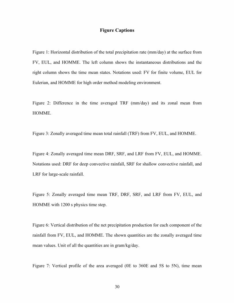
Figure Captions

Figure 1: Horizontal distribution of the total precipitation rate (mm/day) at the surface from

FV, EUL, and HOMME. The left column shows the instantaneous distributions and the

right column shows the time mean states. Notations used: FV for finite volume, EUL for

Eulerian, and HOMME for high order method modeling environment.

Figure 2: Difference in the time averaged TRF (mm/day) and its zonal mean from

HOMME.

Figure 3: Zonally averaged time mean total rainfall (TRF) from FV, EUL, and HOMME.

Figure 4: Zonally averaged time mean DRF, SRF, and LRF from FV, EUL, and HOMME.

Notations used: DRF for deep convective rainfall, SRF for shallow convective rainfall, and

LRF for large-scale rainfall.

Figure 5: Zonally averaged time mean TRF, DRF, SRF, and LRF from FV, EUL, and

HOMME with 1200 s physics time step.

Figure 6: Vertical distribution of the net precipitation production for each component of the

rainfall from FV, EUL, and HOMME. The shown quantities are the zonally averaged time

mean values. Unit of all the quantities are in gram/kg/day.

Figure 7: Vertical profile of the area averaged (0E to 360E and 5S to 5N), time mean

31

precipitation production rate from FV, EUL, and HOMME.

Figure 8: (a) Frequency distribution of daily total rainfall (TRF) in the tropics (0E to 360E

and 10S to 10N) for 90 days from FV, EUL, and HOMME. (b) Amount of TRF falling into

each of the bins from FV, EUL, and HOMME.

Figure 9: Longitude-Time diagrams of daily rainfall (mm/day) averaged between 2.5S -

2.5N from (a) FV, (b) EUL, and (c) HOMME.

Figure 10: Vertical profile of the area averaged (0E to 360E and 2.5S to 2.5N) time mean

moist heating from FV, EUL, and HOMME.

Figure 11: Zonally averaged time mean surface evaporation (mm/day), large-scale moisture

convergence (mm/day), and precipitable water (kg/m2) from FV, EUL, and HOMME.

Figure 12: Zonally averaged time mean moisture deficit (gram/kg) and wind strength (m/s),

at the 1st model level from FV, EUL, and HOMME.

Figure 13: Zonally averaged time mean convective available potential energy (CAPE) from

FV, EUL, and HOMME.

Figure 14: (a) Vertical profile of the area averaged (0E to 360E and 5S to 5N) time mean

relative humidity for (EUL-FV) and (HOMME-FV). (b) Same as figure-a but for specific

humidity. (c) Same as figure-a but for temperature. Notations used: RH for relative

32

humidity, Q for specific humidity, and T for temperature.

Figure 15: Zonally averaged time mean temperature (K) for (a) FV, (b) EUL, and (c)

HOMME.

Figure 16: Zonally averaged time mean zonal wind (m/s) for (a) FV, (b) EUL, and (c)

HOMME.

Figure 17: Zonally averaged time mean pressure vertical velocity (Pa/s) for (a) FV, (b)

EUL, and (c) HOMME

Figure 18: Zonally averaged time mean specific humidity (g/kg) for (a) FV, (b) EUL, and

(c) HOMME.

33

Table Caption

Table 1. Global mean total rainfall (mm/day) from the three dynamical cores.

34

Figures

Figure 1: Horizontal distribution of the total precipitation rate (mm/day) at the surface from

FV, EUL, and HOMME. The left column shows the instantaneous distributions and the

right column shows the time mean states. Notations used: FV for finite volume, EUL for

Eulerian, and HOMME for high order method modeling environment.

35

Figure 2: Difference in the time averaged TRF (mm/day) and its zonal mean from

HOMME.

36

Figure 3: Zonally averaged time mean total rainfall (TRF) from FV, EUL, and HOMME.

37

Figure 4: Zonally averaged time mean DRF, SRF, and LRF from FV, EUL, and HOMME.

Notations used: DRF for deep convective rainfall, SRF for shallow convective rainfall, and

LRF for large-scale rainfall.

38

Figure 5: Zonally averaged time mean TRF, DRF, SRF, and LRF from FV, EUL, and

HOMME with 1200 s physics time step.

39

Figure 6: Vertical distribution of the net precipitation production for each component of the

rainfall from FV, EUL, and HOMME. The shown quantities are the zonally averaged time

mean values. Unit of all the quantities are in gram/kg/day.

40

Figure 7: Vertical profile of the area averaged (0E to 360E and 5S to 5N),

time mean precipitation production rate from FV, EUL, and HOMME.

41

Figure 8: (a) Frequency distribution of daily total rainfall (TRF) in the deep

tropics (0E to 360E and 10S to 10N) for 90 days from FV, EUL, and

HOMME. (b) Amount of TRF falling into each of the bins from FV, EUL,

and HOMME.

42

Figure 9: Longitude-Time diagrams of daily rainfall (mm/day) averaged between 2.5S -

2.5N from (a) FV, (b) EUL, and (c) HOMME.

43

Figure 10: Vertical profile of the area averaged (0E to 360E and 2.5S to 2.5N)

time mean moist heating from FV, EUL, and HOMME.

44

Figure 11: Zonally averaged time mean surface evaporation (mm/day), large-scale moisture

convergence (mm/day), and precipitable water (kg/m2) from FV, EUL, and HOMME.

45

Figure 12: Zonally averaged time mean moisture deficit (gram/kg) and wind strength (m/s),

at the 1st model level from FV, EUL, and HOMME.

46

Figure 13: Zonally averaged time mean convective available potential energy (CAPE) from

FV, EUL, and HOMME.

47

Figure 14: (a) Vertical profile of the area averaged (0E to 360E and 5S to 5N) time mean

relative humidity for (EUL-FV) and (HOMME-FV). (b) Same as figure-a but for specific

humidity. (c) Same as figure-a but for temperature. Notations used: RH for relative

humidity, Q for specific humidity, and T for temperature.

48

Figure 15: Zonally averaged time mean temperature (K) for (a) FV, (b) EUL, and (c)

HOMME.

49

Figure 16: Zonally averaged time mean zonal wind (m/s) for (a) FV, (b) EUL, and (c)

HOMME.

50

Figure 17: Zonally averaged time mean pressure vertical velocity (Pa/s) for (a) FV, (b)

EUL, and (c) HOMME.

51

Figure 18: Zonally averaged time mean specific humidity (g/kg) for (a) FV, (b) EUL, and

(c) HOMME.

52

Table

Dynamical Core Global Mean TRF

FV 2.888

EUL 3.024

HOMME 2.948

Table 1. Global mean total rainfall (mm/day) from the three dynamical cores.