Evaluation of the effectiveness of methods of the ... · The classical solution to ... while the question of the economic effectiveness ... that the use of currency-based derivatives

Original Article

Evaluation of the effectiveness of methods of the

imperfect hedging of financial options on the

Russian forward marketReceived (in revised form): 14th January 2014

Varvara Nazarova

obtained his PhD and is Researcher and Associate Professor in the Department of Financial Markets andFinancial Management at National Research University Higher School of Economics in Saint Petersburg, Russia.His fields of interest are risk-management, financial management, value‐based management and socialoutcomes evaluation.

Correspondence: Varvara Nazarova, National Research University Higher School of Economics, Russia

ABSTRACT Under unstable economic conditions, interest in the financial derivativesmarket is easy to understand. On the Russian forward market, derivatives such as optionsand futures are gaining increasing popularity as a means of managing the risks of businessunits in order to protect against possible financial losses. The competition created among theorganizers of forward trading has encouraged the emergence of a technically effective trad-ing method and an expanded range of available financial instruments. The need for anexpanded range of risk-management instruments and the introduction onto the market ofcutting-edge methods relying on a strict formalization of investor decisions has determinedthe current relevance of the article at hand. The aim of the article involves studying the latestmethods of hedging financial options, comparing and contrasting the new methods withthose traditionally used in the financial industry, and analyzing the opportunities forapplying methods of imperfect hedging on the Russian forward market.

Journal of Derivatives & Hedge Funds (2014) 20, 28–51. doi:10.1057/jdhf.2014.6;published online 20 February 2014

Keywords: option market; Russian forward market; quantile hedging; imperfect hedging; risks andriskiness of investments; market portfolio

INTRODUCTION

The problem of hedging operations involvingderivatives is an issue of pressing concern for thedomestic financial sciences. Real economic needsdemand that the organizers and leading operatorsof the forward market engineer a significantnumber of new financial instruments capableof hedging the majority of operations conducted

on the cash market. While the Russian futuresmarket has largely formed, the market forfinancial options providing more flexibleopportunities to manage risk is still in its infancy.The need for an expanded circle ofrisk-management instruments and the practicalincorporation into the work of professionalmembers of the Russian forward market of

© 2014 Macmillan Publishers Ltd. 1753-9641 Journal of Derivatives & Hedge Funds Vol. 20, 1, 28–51www.palgrave-journals.com/jdhf/

http://dx.doi.org/10.1057/jdhf.2014.6

http://www.palgrave-journals.com/jdhf

methods of scientific risk management basedon a strict formalization of investment decisionsdetermines the current relevance of thisdissertation topic. The classical solution tothe problem of hedging financial options isprovided within the scope of the concept ofperfect hedging. Its foundations were laid bythe well-known works of Black and Scholes(1973) and Merton (1973).The concept of perfect hedging is aimed at

engineering a certain portfolio of marketassets that generates payouts consistent with thepayouts of a given derivative. In the absence ofarbitration, the cost of the portfolio determinesthe cost of the derivative. As of today, thestrategies of perfect hedging have been borneout as a standard approach of financialengineering earning broad recognition in thetheory and practice of risk management. Theirmain distinguishing feature lies in the fact thatthe cost of the financial option is determinedindependently of the preferences andcharacteristics of its owner. Methods ofperfect hedging do not take into account theexpectations of the owner of the forwardposition, his attitude toward risk or the nuancesof his particular investment strategy (Allayannisand Weston, 1998).The new approach to risk management offers

methods of the imperfect hedging of financialoptions (the imperfect hedge). Their criticaldistinction involves the construction of a hedgingstrategy that deliberately allows for the possibilityof the onset of losses (Géczy et al, 1997). Thanksto this, capital is freed up at a controlled risklevel, thereby creating the opportunity for newfinancial operations. As a result, capital is freed upat a controlled level for new financial operations,which opens up additional risk-managementopportunities for the overall investment strategy.

The undeniable advantage of methods ofimperfect hedging lies in the ability they provideto take into account the expectations of themarket participants and his attitude toward risk.In the practical sense, for the economic agentinclined toward active action on the forwardmarket and prepared to expose himself tocontrolled risk, methods of imperfect hedgingpresent new instruments for the support ofinvestment decisions.Despite the above-listed advantages of

methods of imperfect hedging, the first stepstoward their theoretical conceptualizationwere only taken in the 1990s in the works ofDuffie and Richardson (1991), Melnikov andNechaev (1998) and Foellmer and Leukert(1999, 2000). Moreover, these studies wereaimed at finding a mathematical solution tothe problem of engineering an imperfect hedge,while the question of the economic effectivenessof imperfect hedging was largely neglected.Unlike the futures market, the financial

options market, which offers greateropportunities for the management of financialrisks, began its formation in our countryrelatively recently. Despite the obvious strengthsof methods of imperfect hedging, such methodshave yet to find broad application on theRussian forward market. This is largelyassociated with the fact that research intomethods of the imperfect hedging of financialoptions only got its start in the last decade ofthe last century.This determined the need for detailed

theoretical and practical analysis of the methodsof imperfect hedging, as well as empirical studieson issues related to the practical application ofsuch methods. The conducting of such studies isa necessary predicate for the integration ofrisk-management methods into the practical

Imperfect hedging in the Russian forward market

29© 2014 Macmillan Publishers Ltd. 1753-9641 Journal of Derivatives & Hedge Funds Vol. 20, 1, 28–51

work of participants of the Russian forwardmarket.The object of this study is the Russian forward

market, and the subject – the price risks faced bythe holder of a forward position.The information base of this study

encompasses data from the Russian TradingSystem (RTS) Stock Exchange (www.rts.ru),the Moscow Interbank Currency Exchange(www.micex.ru), the Bank for InternationalSettlements (www.bis.org) and the Bank ofRussia (www.cbr.ru).Selected as the methodological basis for

the study were system analysis, methods ofgeneralization and comparison, the methodsof mathematical and statistical analysis, and thetheory of probability.The theoretical basis for the work is provided

by the generally accepted provisions of the theoryof hedging and the price formation of derivativeinstruments, as well as financial engineering, thetheory of risk management, the theory offinancial markets and the securities market. Thesolution of specific problems featured the useof the methods of probably theory, specifically,the theory of stochastic (random) processes, aswell as the concept of the computer modeling offinancial markets, as proposed and demonstratedby a number of academics and stock marketpractitioners. A key role in identification of theproblem area was played by the works ofF. Black, M. Scholes, R. Merton, A.V. Melnikov(1998), N.I. Berzon, M. Harrison, S. R. Pliska,H. Foellmer, and others. Harrison and Pliska(1983) show in their papers that the financialmarket is complete if, besides physical probabilitymeasure, there is its equivalent martingalemeasure. Risk-neutral measure implies that aderivative’s price is determined by equivalent realphysical probability measure.

In his papers, Berzon (2003) presents specificfeatures of the Russian derivatives marketfunctioning, basic investment strategies, advantagesand disadvantages of hedging mechanisms asapplied to the Russian derivatives market.The scientific novelty of the study is determined

by its development of theoretical views in thearea of the hedging of financial options and itseconomic justification for the possibility of usingmethods of imperfect hedging in practice.The theoretical significance of the study lies in

the fact that it manages to clarify the economiccontent of methods of imperfect hedging andjustify their selection depending on theexpectations and risk attitude of the economicagent and the particularities of the given market.The practical importance of the study rests onthe fact that the yielded results can be applied byparticipants on the forward market in the processof hedging and derivative-portfolio management(Mun, 2002).Empirical studies have confirmed that

the practical application of risk-managementmethods facilitates the commercial successof individual companies. For example,the work by Géczy et al (1997) establishedthat the use of currency-based derivativeshas a positive effect on the growth potentialof a company, as measured in terms ofresearch-and-development and engineeringadvancements. The work by Allayannisand Weston (1998) established a directdependency between the use of hedgingmethods and company value, as measuredwith the help of Tobin’s Q ratio. In thepast 5 years, however, precious little workhas been written on imperfect hedging.Derivative instruments are an important

means of achieving the goals of individual risk-management strategy. Like any other instrument,

Nazarova

30 © 2014 Macmillan Publishers Ltd. 1753-9641 Journal of Derivatives & Hedge Funds Vol. 20, 1, 28–51

www.rts.ru

www.micex.ru

www.bis.org

www.cbr.ru

however, they are only useful to the extent thattheir possibilities and limits are known (modelrisk, credit risk and liquidity risk). It is thereforeof critical importance that when using derivatives,market participants have a thoroughunderstanding of the structuring of forwardcontracts, the dependence between theiryield and risk, and how they react to changesin economic conditions. A well-balancedrisk-management strategy, reconciled with thecompany’s commercial goals and confirmed byreliable empirical studies, is a necessary conditionfor the use of derivative financial instruments.The exchange-traded and over-the-counter

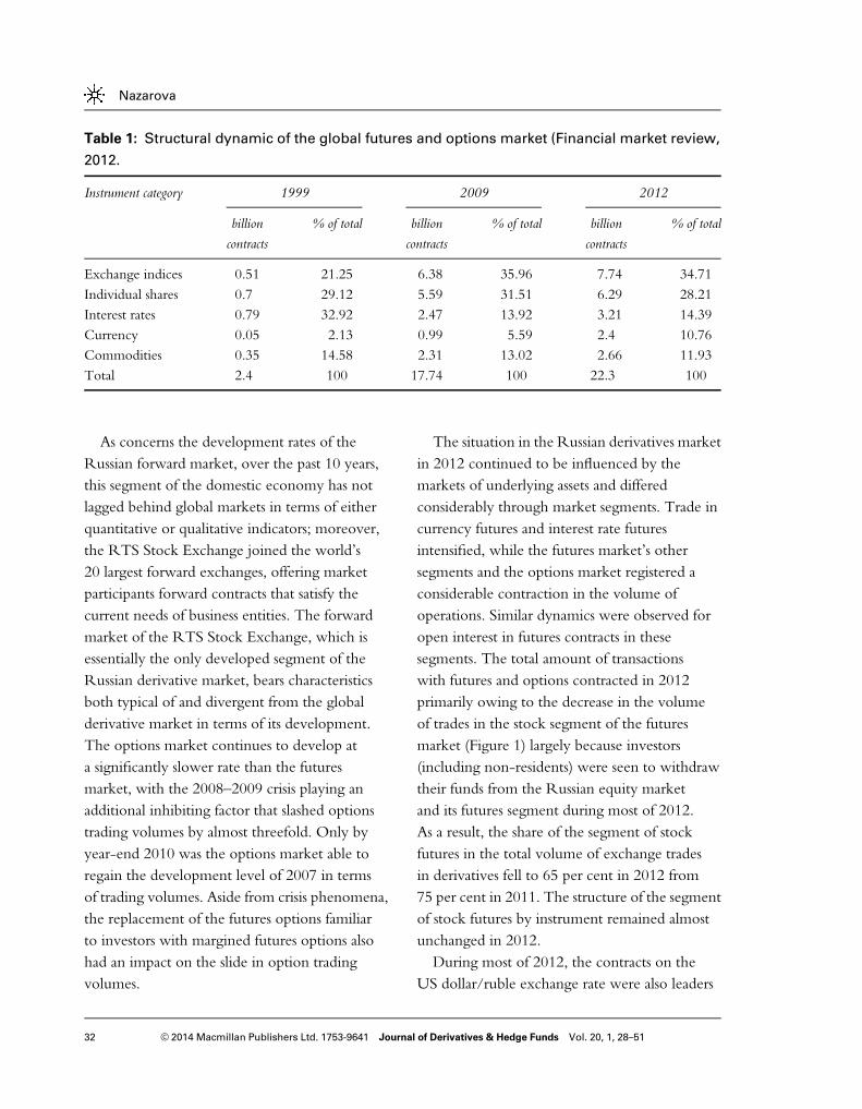
segments of the global derivatives market begantheir active and uninterrupted development withthe introduction in the early 1970s of derivativesfor financial assets. This growth continued ata brisk pace until 2009, during which the marketonly managed to preserve achieved tradingvolumes. Nevertheless, in 2010, the globalmarket for exchange-traded derivatives returnedto its pre-crisis growth rate, demonstratingan annual turnover gain of 26 per cent – just2 per cent short of the gain achieved in 2007.Global trading volumes in standard contractsexperienced an almost tenfold increase, growingfrom 2.4 billion contracts in 1999 to 22.3 billioncontracts in 2010. The geographical structure ofthe derivatives market also underwent change.If, by the early 2000s, the undisputedforward-trading leaders were the USA and thecountries of Western Europe, the leader for thepast several years has been the Korean exchange.Trailing the leader by a slim margin are the USforward exchanges that merged at the turn of thecentury. Behind the leader by almost 1 billioncontracts are the American-European forwardexchange alliances EUREX and NYSEEuronext. The top-10 world exchanges trading

in futures and options now include the exchangesof India, Brazil and China. The RTS StockExchange has been posting consistently highgrowth rates in terms of trading volume,occupying 11th place on the list of the world’sleading forward exchanges by year-end 2010 andtrailing the Korean exchange in terms of tradingvolume by a factor of 6.4. (Financial marketreview, 2012)The basic elements of consistently high

turnover growth on the world market for futuresand options are as follows:

● The intensive gain in trading volumes on theforward-contract markets in the Asia-PacificRegion and Latin America (42.8 per cent and49.6 per cent in 2010 over 2009), includingthe fact that the Zhengzhou and Shanghaiexchanges (China) demonstrated maximumgrowth in terms of trading in commodityfutures. At the two largest trading platformsin India, turnover in currency futures almosttripled. On the whole, the briskest gain inderivative-trading volume was posted byIndian exchanges – 142 per cent in 2010compared to the previous period.

● The gradual recovery of volumes in theinterest rate derivatives segment, which formany years had occupied lead positions interms of trading volumes among derivativemarkets (information on the distribution oftrading volumes is presented in Table 1) butslipped by 23 per cent in 2009 compared to2008, when the underlying-asset market wasin deep crisis.

● The preservation of high growth rates incommodity-futures trading, wherein themarket players in emerging markets arechiefly interested in agricultural productsand non-ferrous metals.



As concerns the development rates of theRussian forward market, over the past 10 years,this segment of the domestic economy has notlagged behind global markets in terms of eitherquantitative or qualitative indicators; moreover,the RTS Stock Exchange joined the world’s20 largest forward exchanges, offering marketparticipants forward contracts that satisfy thecurrent needs of business entities. The forwardmarket of the RTS Stock Exchange, which isessentially the only developed segment of theRussian derivative market, bears characteristicsboth typical of and divergent from the globalderivative market in terms of its development.The options market continues to develop ata significantly slower rate than the futuresmarket, with the 2008–2009 crisis playing anadditional inhibiting factor that slashed optionstrading volumes by almost threefold. Only byyear-end 2010 was the options market able toregain the development level of 2007 in termsof trading volumes. Aside from crisis phenomena,the replacement of the futures options familiarto investors with margined futures options alsohad an impact on the slide in option tradingvolumes.

The situation in the Russian derivatives marketin 2012 continued to be influenced by themarkets of underlying assets and differedconsiderably through market segments. Trade incurrency futures and interest rate futuresintensified, while the futures market’s othersegments and the options market registered aconsiderable contraction in the volume ofoperations. Similar dynamics were observed foropen interest in futures contracts in thesesegments. The total amount of transactionswith futures and options contracted in 2012primarily owing to the decrease in the volumeof trades in the stock segment of the futuresmarket (Figure 1) largely because investors(including non-residents) were seen to withdrawtheir funds from the Russian equity marketand its futures segment during most of 2012.As a result, the share of the segment of stockfutures in the total volume of exchange tradesin derivatives fell to 65 per cent in 2012 from75 per cent in 2011. The structure of the segmentof stock futures by instrument remained almostunchanged in 2012.During most of 2012, the contracts on the

US dollar/ruble exchange rate were also leaders

Table 1: Structural dynamic of the global futures and options market (Financial market review,

2012.

Instrument category 1999 2009 2012

billioncontracts

% of total billioncontracts

% of total billioncontracts

% of total

Exchange indices 0.51 21.25 6.38 35.96 7.74 34.71

Individual shares 0.7 29.12 5.59 31.51 6.29 28.21Interest rates 0.79 32.92 2.47 13.92 3.21 14.39Currency 0.05 2.13 0.99 5.59 2.4 10.76Commodities 0.35 14.58 2.31 13.02 2.66 11.93Total 2.4 100 17.74 100 22.3 100

Nazarova


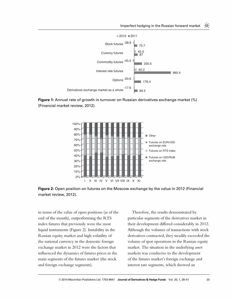
in terms of the value of open positions (as of theend of the month), outperforming the RTSindex futures that previously were the mostliquid instruments (Figure 2). Instability in theRussian equity market and high volatility ofthe national currency in the domestic foreignexchange market in 2012 were the factors thatinfluenced the dynamics of futures prices in themain segments of the futures market (the stockand foreign exchange segments).

Therefore, the results demonstrated byparticular segments of the derivatives market intheir development differed considerably in 2012.Although the volumes of transactions with stockderivatives contracted, they steadily exceeded thevolume of spot operations in the Russian equitymarket. The situation in the underlying assetmarkets was conducive to the developmentof the futures market’s foreign exchange andinterest rate segments, which showed an

84.5

176.4

960.4

200.5

87

75.7

-17.6

-20.6

62.2

-45.5

42.5

-28.8

Derivatives exchange market as a whole

Options

Interest rate futures

Commodity futures

Curency futures

Stock futures

2012 2011

Figure 1: Annual rate of growth in turnover on Russian derivatives exchange market (%)

(Financial market review, 2012).

0%

10%

20%

30%

40%

50%

60%

70%

80%

90%

100%

I II III IV V VI VII VIII IX X XI

Other

Futures on EUR/USDexchange rate

Futures on RTS index

Futures on USD/RUBexchange rate

Figure 2: Open position on futures on the Moscow exchange by the value in 2012 (Financial

market review, 2012).



increase in the volume of trades and openpositions (in contracts) (Financial marketreview, 2012).

PRINCIPLE OF THE METHOD

The methods of imperfect hedging provide anopportunity to lower the cost of protecting againstrisk via the assumption of a certain controlled riskof the onset of losses. The traditional decision-making model assumes that, all other things beingequal, the rational investor will always prefergreater profit to lesser. The rational marketparticipant also avoids excessive riskiness and isonly prepared to accept it in exchange forcompensation, namely in the form of high yield.It is precisely for this reason that managing the riskof an options contract consists of maximizinganticipated yield at a controlled level of risk, or,equivalently, minimizing risk at the desired levelof yield. The foregoing is the main principle anddistinguishing feature of methods of the imperfecthedging of financial options.The structure of the open option position serves

as the source of risk. By modifying this structure,the risk manager gains the opportunity to controlthe level of uncertainty. By using the assumptionthat an option payout will sometimes not bemade or not made in full, the costs involved inimplementing the replication strategy will decreaseowing to the risk of the onset of losses in suchcases. The crucial task in such situations is todetermine the conditions under which therejection of replication entails the lowest riskincrease and the greatest growth in desired yield.Methods of the imperfect hedging of financial

options are divided into three groups, dependingon the method of risk control – the mean-squarehedging method, the quantile-hedging methodand the expected-shortfall hedging method.

The mean-square hedging method is one ofthe most studied methods of the imperfecthedging of financial options. This method isdistinctive in that the ‘quality measurement’ ofthe hedging strategy is taken with the help of thesquared difference of terminal capital and thepayment obligation. This method was proposedand described in the studies by Duffie andRichardson in 1991,and received furtherdevelopment in the studies by Melnikov andNechaev in 1998 and the work by Schweizerin 1999.Mean-square hedging makes it possible to

lower the costs of option hedging in a controlledfashion, but the method does have the drawbacksinherent in all quadratic risk measures – namelythat strategic risk increases after both positiveand negative payout deviations. Insofar as thismethod has been outlined in detail in variousstudies and is well known, our study eschewsits review in favor of a consideration of theother methods of the imperfect hedging offinancial options.The next group of methods for the hedging of

financial options is quantile hedging. The cost ofan option in the case of quantile hedging iscalculated as the result of the interaction of atotality of factors whose unforeseeable changedynamic determines the hedger risk. This hedgerrisk consists of the unpredictability of marketdynamics or uncontrollable changes in theeconomic environment and relates to the groupof market risks.The concept of Value-at-Risk is frequently

used as a measure of market risk. The principlebehind this concept lies in its determination ofloss amount at the pre-determined confidenceinterval. More formally, the method boils downto identifying the quantile of profit and lossdistribution anticipated at a certain point in time

Nazarova


in the future. When designating confidenceinterval via ε, Value-at-Risk corresponds to thelower quantile of order 1−ε. This methodprovides a detailed understanding of the riskentailed by the forward position, makes itpossible to measure the economic cost of theforward position and makes an allowance forcomparisons with related risk measures.When using the Value-at-Risk concept as

a measure of risk, the task of identifying theoptimal risk-return distribution is relegated to thefield of the general theory of statistical confidenceevaluation. The basic principle of this theory isthe quantile or threshold of the evaluation area ata pre-determined interval. It is precisely for thisreason that this method of the imperfect hedgingof financial options, in which the quantile fordistributing the profit or loss of the hedgingstrategy is used as the success criterion, is referredto as quantile.Our study provides a description of the strategy

behind the quantile-hedging method, whichmaximizes the natural probability of successfulhedging while limiting the costs involved instrategy implementation. The idea of quantilehedging is still quite new, and has yet to bedescribed systematically in sufficient detail inthe respective literature. The concept was firstintroduced by H. Foellmer (1999) in March of1995 within the framework of the traditionalBlack–Scholes model, while the critical features ofthe method were elucidated in the study byFoellmer and Leukert in 1999. In this study, theproblem of the quantile-hedging method isconsidered from the mathematical standpoint. Theproblem is solved by generalizing the Kulldorfmethod (1993) in order to maximize theprobability of achieving a certain level ofBrownian motion by the pre-determinedmoment in time. By applying such a generalized

abstract method, the researchers were able toelucidate the solution to the problem relativelysuccinctly. However, the economic content of themodel remained beyond the scope of the evidencepresented in their theory.It must be noted that the quantile-hedging

method only takes into account the probabilityof the onset of losses, but fails to consider theiramount. Positions with extremely high and verylow loss values are assumed to be equally risky.From the practical standpoint, such an approachis incomplete and deserving of serious criticism.The third group of methods for the imperfect

hedging of financial options consists of expected-shortfall hedging. This concept takes into accountthe amount of anticipated losses, which is unlikethe preceding method, in which everything islimited by the control over the probability of lossonset. This method determines risk as themathematical expectation of a shortfall whileproviding a physical measure of probability andminimizing this risk in a way that limits the costof hedging. The main idea behind the expected-shortfall hedging method is described in the studyby Fellmer and Likert published in 2000. In theirstudy, the authors chiefly concentrated on themathematical formulation of this problem.The above-described methods of imperfect

hedging (quantile hedging and expected-shortfallhedging) are frequently described in varioussources as rather similar models of imperfecthedging. The comparison of these methodsprovided in our study indicates that a hedgingstrategy can only be optimal under both criteriaprovided the observance of certain conditions. Ingeneral, the structure of the set of hedgedpositions depends on the method applied. It isprecisely for this reason that a hedging portfoliooptimal in terms of one criterion is often less thanoptimal in terms of another criterion.



METHODOLOGY

From a practical standpoint, the significantdistinction among methods for the imperfecthedging of financial options within theframework of the Black–Scholes model involvestheir use of a combination of a certain number ofoptions of different types and different priceexecution. That said, the combination dependson such model parameters as volatility, averagegrowth rate and bank interest rate. When usingimperfect hedging within the framework of theBlack–Scholes model, two option-executionprices are applied:

● K – execution price, equal to the price of theunderlying asset at the start of the hedgingperiod, and

● h – threshold, calculated according to thefollowing formula:

h ¼ eσ�b + lnðS0 + ðr + 12�σ2ÞT ;

where

b ¼ffiffiffiffiT

p�N - 1ð1 - εÞ + μ - r

σ� T ;

μ – average growth rate of the underlying asset,r – bank interest rate, σ – volatility, Т – executiontime, S – asset price, ε – probability of the onsetof losses and N – the function of standard normaldistribution.

Algorithm of successful hedging

Depending on model parameters, the set ofsuccessful hedging will become distinct andthreshold h will be used differently, as shall bedescribed below. Thus, in order to select theright hedging strategy, it is important to adhere tothe following algorithm:Step 1. Identification of the structure of successfulhedging set based on option type and parameters

such as volatility, average growth rate and thebank interest rate.Step 2. Determination of hedging strategy payoutwithin the hedging strategy set.Step 3. Selection of the method of replication forhedging strategy payouts.

Set of successful hedging

In our study, we consider two methods of theimperfect hedging of financial options – thequantile-hedging method and the expected-shortfall hedging method. Both of these methodslower the cost of hedging by allowing for the riskof loss onset.The main distinction between these methods

lies in their different methods for determiningrisk. Under quantile hedging, risk is determinedas the probability of the onset of losses. In theexpected-shortfall model, risk is determined asanticipated losses.As has been described, methods of imperfect

hedging assume the use of a combination ofseveral options. The structure of thiscombination depends on hedging method andmodel parameters. Structure determination isinfluenced by such indicators as volatility σ,growth rate μ and interest rate r. Figure 3illustrates various combinations of theseparameters, which determine the set of successfulhedging.As the figure indicates, three variants are

possible for the shape of the set of successfulhedging. Let us consider these cases using theexample of an option call. Under quantilehedging, set shape changes depending on theexpression (μ−r)/σ2 – that is, whether or not theexpression exceeds 1. In the first variant, the setconsists of two fields. The first field consists of aposition with a low asset quote approximating

Nazarova


the price of option execution. Threshold h1constrains this field from above. The second fieldencompasses positions in which the pricing of theunderlying asset is higher than threshold h1, itmeans threshold h2 (h2>h1). If the expression(μ−r)/σ2<1 (threshold h2 and threshold h3),the set also encompasses positions at pricingbelow threshold h3. Under the expected-shortfallhedging method, set shape is determined bythe difference between μ and r. At μ>r(thresholds h1 and h2), payouts are made atpositions to the right of some border h4;otherwise (threshold h1), a limitation is ineffect above threshold h5. Table 2 presentsall possible structures of the set of successfulhedging depending on different modelparameters using the option call example.Based on the choice of hedging method, set

structure is presented differently in the first andsecond fields. In these fields, average growth rateis higher than the bank interest rate. In this case,hedging strategy will only be optimal under oneof the risk parameters – quantile or expectedshortfall. Yet, if the growth rate is not higherthan the bank interest rate, the sets of hedging

strategies coincide. In this case, under strategyoptimality for one criterion, the strategy becomesoptimal under the other risk criterion. Thesituation in which interest rate is lower than thegrowth rate of the underlying asset is frequentlyobserved on the market.As a method for the empirical testing of

hedging concepts, an empirical study wasconducted on the basis of one of the commonlyaccepted hedging methods – delta hedging. Thismethod is rather simple, which explains its broaduse. The principle behind the method is asfollows: a certain portfolio consisting of anunderlying risky asset and bank account (credit) isused to dynamically reproduce the paymentfunction of the forward contract. That said, thepercentage of shares or other risky asset in theabove-mentioned portfolio coincides with thisindicator as the option delta (one of the ‘Greek’indicators in the Black–Scholes model).The option delta is the ratio of change in

option price, expressed as the change in price ofthe underlying risky asset to the change in priceof the risky asset. Mathematically speaking,the option delta indicator can be viewed as thefirst-order derivative of the cost of the optionfor the asset underlying the option. Just as anyfirst-order derivative, this indicator reflects the

Table 2: Set of the successful hedging of an

option call, depending on model parameters

Field Dependency Quantilehedging

Expected-shortfallhedging

I (μ−r)/σ2>1 (0;h1]∩[h2;∞) [h4;∞)II (μ−r)/

σ2⩽1∩μ>r(0;h3] [h4;∞)

III μ⩽r (0;h3] (0;h5]

Figure 3: Set of successful hedging.



speed of change in option cost relative to theprice dynamic of the underlying asset.To start, let us take a closer look at the

algorithm for delta hedging. A firm grasp of thissimple, perfect model is crucial to the furtherexploration of imperfect hedging methods. Weshall consider the mechanism of delta hedgingusing an option call in the Black–Scholes model.Aside from this model, other, more perfectmethods of dynamic hedging exist that functionin discreet time, but within the scope of ourinvestigation we shall use the Black–Scholesmodel in particular, insofar as it illustrates themechanisms behind imperfect-hedging methodsto a sufficient extent while remaining quitesimple.In this model, the delta indicator represents the

value of the function of standard normaldistribution from coefficient d1, whoseidentification formula is presented below,together with the formula for identifying thecoefficient of the option call delta:

Δi ¼ 1

σffiffiffiffiffi2π

p e -ðd1 - μÞ2

2σ2 ;

where

d1 ¼ln Si

x

� �+ r + 1

2 σ2

� �T

σffiffiffiffiT

p ;

where Si – current asset price, Т – execution timein years, r – interest rate, σ – volatility,μ – average growth rate and x – option executionprice.The algorithm for delta hedging is quite simple

and can be described using the following stages ofits implementation:

1. At the time of issuance, the option call has aprice that can be found using the Black–Scholes formula, as presented below:

C0ðxÞ ¼ S0 �N d1ðxÞð Þ - x � e- rT �Nðd2 xð Þ;

where

d1ðxÞ ¼ln Si

x

� �+ r + 1

2 σ2

� �T

σffiffiffiffiT

p ;

d2ðxÞ ¼ d1ðxÞ - σ �ffiffiffiffiT

p:

2. For the purposes of hedging, the portfolio isaugmented with the purchase of a risky assetin an amount commensurate with theindicator for the option call delta.

3. Financing for the purchase of the asset into theportfolio is secured using two sources: thepremium yielded on the option and a bankcredit under interest rate r, expressed as annualinterest.

4. By the end of the first day of hedging, theportfolio is loaded with the delta of sharenumber (or other risky asset) and credit B,whose amount is determined as the differencebetween the cost of the purchased shares andthe premium yielded on the option. Theformula for calculating the amount of bankcredit is presented below:

B0 ¼ Δ0 � S0 -CBS0 ;

where C0BS – price of the option call,

calculated according to the formula providedin the preceding point.

5. That said, the cost of the entire hedgingportfolio is the sum total of the cost of theshares and the amount of the bank credit. Itwould be logical to note that on the first dayof hedging, the cost of the option is equal tothe cost of the hedging portfolio, which iseasy to understand by inserting the formulafrom the fourth point into the formula fromthe fifth point.

Beginning on the second day of hedging,the actions unfold somewhat differently: let usassume that the pricing of the risky asset haschanged. Let us further assume that validity

Nazarova


period of the forward contract has shortenedby 1 day. Both of these indicators result in achange in the indicator for the option call delta,therefore the hedging portfolio must be adjusted.Adjustment of the hedging portfolio occurs asfollows:

1. In the case of a positive change in the price ofthe underlying asset the option call delta alsoincreases, therefore the portfolio should beaugmented with the purchase of shares in anamount equal to the increment of the indica-tor for the option call delta. In this case, cost ofpurchase is the product of the increment ofthe option call delta times the current price ofthe underlying asset. This purchase is alsofinanced using additional credit, meaning thatthe amount of credit increases. The hedgermust also pay interest to the bank for his use ofthe credit funds on the first day of hedging.Interest amount is calculated according to thefollowing formula:

r � B0 � dt:Consequently, the amount of bank creditincreases to the sum calculated according tothe following formula:

B1 ¼ B0 + r � B0 � dt + Δ1 -Δ0ð Þ � S1:2. In the case of a negative dynamic in the

pricing of the underlying asset, adjustment ofthe hedging portfolio occurs similarly, withthe sole exception that as a result of thenegative change in the coefficient for theoption call delta, a certain number of sharesfrom the hedging portfolio must be sold, as aresult of which the amount of bank creditdecreases. As a result of such adjustments, thecost of the hedging portfolio totals the sumcalculated according to the following formula:

π1 ¼ Δ1 � S1 +B1:

The cost of the hedging portfolio maynot equal the theoretical cost of the optioncall according to the Black–Scholes formulaowing to a phenomenon known as hedgingerror. Hedging error may occur as a resultof the fact that the dependency of optionprice on a change in the price of the risky assetunderlying the derivative is not a linear function,whereas delta hedging only covers the linearelement of the change in option price. Thisdivergence between the theory and practiceof managing financial risks also occurs dueto the fact that in theory, portfolio parametersare found in the continuous model, whereas inpractice, hedging occurs at a discrete moment intime.Presented above are the formulae and

algorithm for adjusting the hedging portfolio onthe second day of hedging. Insofar as due to thechange in price of the underlying asset and thechange in the time to maturity of the option, oneach of the subsequent days, the portfolio mustbe adjusted and the relative weight of all ofthe elements of the hedging portfolio must bereviewed, for subsequent days, the amount ofbank credit and total cost of the hedging portfoliocan be represented in the form of the followingformulae:

Bt ¼ Bt - dt + r � Bt - dt � dt + ðΔt -Δt - dtÞ � St:

πt ¼ Δt � St +Bt:

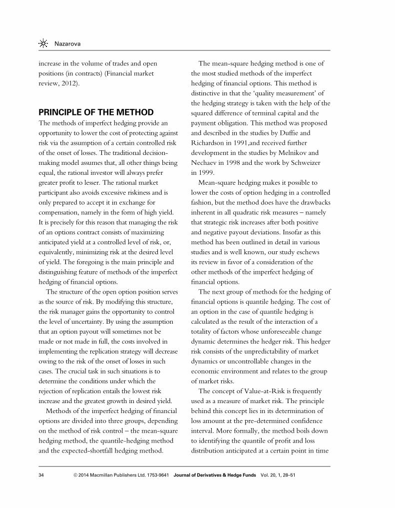
The position under the risky asset is liquidatedwhen the moment of execution of the forwardcontract approaches. The proceeds yieldedfrom the sale of the asset go toward dischargingthe debt under the bank credit. Let us nowillustrate the mechanism behind delta hedgingwith the aid of the arrangement presented inFigure 4.



EMPIRICAL RESULTS

Empirical testing of the different methodsof hedging is conducted on the basis of thequotes for shares and other risky assetsparticipating in the FORTS system (forwardmarket) on the RTS Exchange in Moscow. Tostart, we must identify such market indicators asvolatility and average rate of growth in asset priceneeded to calculate the price of the option call.Share volatility – a statistical financial indicatorthat characterizes average annual change(fluctuation) in asset price or price variability.Volatility is a critical indicator in the field of riskmanagement, insofar as it indicates the measureof risk involved in using certain financialinstruments within a pre-determined period oftime. Volatility is the mean-square (standard)deviation in price divided by the square root ofthe time period, expressed in years. The formula

for calculating average annual volatility ispresented below:

σ ¼ffiffiffiffiffiffiffiffiffiffiffiffiffiffiffiffiffiffiffiffiffiffiffiffiffiffiffiffiffiffi1n

Pni¼1 ðSi - SÞ2

qffiffiffiP

p ;

where

S ¼Pn

i¼1 Sin

;

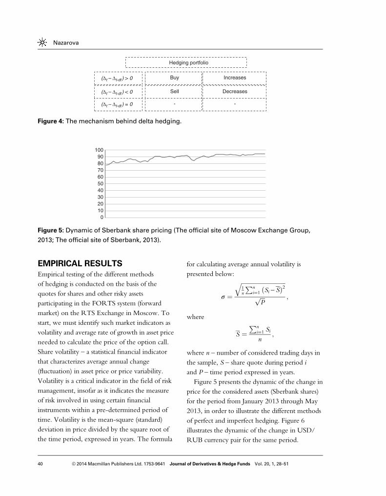
where n – number of considered trading days inthe sample, S – share quote during period iand P – time period expressed in years.Figure 5 presents the dynamic of the change in

price for the considered assets (Sberbank shares)for the period from January 2013 through May2013, in order to illustrate the different methodsof perfect and imperfect hedging. Figure 6illustrates the dynamic of the change in USD/RUB currency pair for the same period.

0102030405060708090

100

Figure 5: Dynamic of Sberbank share pricing (The official site of Moscow Exchange Group,

2013; The official site of Sberbank, 2013).

Hedging portfolio

Underlying asset BankcreditBuy Increases

Sell Decreases

- -

(Δt – Δt-dt ) > 0

(Δt – Δt-dt ) < 0

(Δt – Δt-dt ) = 0

Figure 4: The mechanism behind delta hedging.

Nazarova


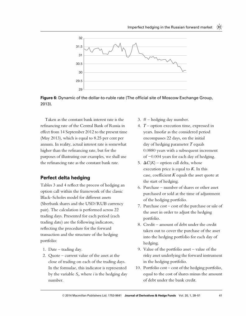
Taken as the constant bank interest rate is therefinancing rate of the Central Bank of Russia ineffect from 14 September 2012 to the present time(May 2013), which is equal to 8.25 per cent perannum. In reality, actual interest rate is somewhathigher than the refinancing rate, but for thepurposes of illustrating our examples, we shall usethe refinancing rate as the constant bank rate.

Perfect delta hedging

Tables 3 and 4 reflect the process of hedging anoption call within the framework of the classicBlack–Scholes model for different assets(Sberbank shares and the USD/RUB currencypair). The calculation is performed across 22trading days. Presented for each period (eachtrading date) are the following indicators,reflecting the procedure for the forwardtransaction and the structure of the hedgingportfolio:

1. Date – trading day.2. Quote – current value of the asset at the

close of trading on each of the trading days.In the formulae, this indicator is representedby the variable Si, where i is the hedging daynumber.

3. # – hedging day number.4. Т – option execution time, expressed in

years. Insofar as the considered periodencompasses 22 days, on the initialday of hedging parameter Т equals0.0880 years with a subsequent incrementof −0.004 years for each day of hedging.

5. ΔС(K) – option call delta, whoseexecution price is equal to К. In thiscase, coefficient К equals the asset quote atthe start of hedging.

6. Purchase – number of shares or other assetpurchased or sold at the time of adjustmentof the hedging portfolio.

7. Purchase cost – cost of the purchase or sale ofthe asset in order to adjust the hedgingportfolio.

8. Credit – amount of debt under the credittaken out to cover the purchase of the assetinto the hedging portfolio for each day ofhedging.

9. Value of the portfolio asset – value of therisky asset underlying the forward instrumentin the hedging portfolio.

10. Portfolio cost – cost of the hedging portfolio,equal to the cost of shares minus the amountof debt under the bank credit.

29

29.5

30

30.5

31

31.5

32

Figure 6: Dynamic of the dollar-to-ruble rate (The official site of Moscow Exchange Group,

2013).



Quantile hedging

Tables 5 and 6 present the procedure for quantilehedging, one of the considered methods forthe imperfect hedging of financial options.The technical distinction between the

procedure for quantile hedging within theframework of the Black–Scholes model and themethod for perfect delta hedging consists of thefollowing:

1. Insofar as the ratio (μ−r)/σ2 (μ – averagegrowth in asset value, r – interest rate,

σ – volatility) is less than the identity in bothcases (Sberbank shares and the USD/RUBcurrency pair), the structure of the hedgingportfolio within the framework of themodel for quantile hedging will consistof a combination of three options: twostandard option calls СТ(К) and СТ(h) withthe respective execution prices К and h (upperthreshold his calculated according to theformula described in the second chapter ofour study) and binary option CoNT(h) withexecution price h.

Table 3: Perfect delta hedging using the example of Sberbank shares

Quote # T ΔС(K) Purchase Purchasecost

Creditamount

Value of theportfolio asset

Portfoliocost

92.62 0 0.088 0.5034 0.5034 46.6218 45.0742 46.6218 1.547692.69 1 0.084 0.5035 0.0001 0.0138 45.1042 46.6708 1.5666

92.73 2 0.08 0.5035 0.0000 0.0018 45.1222 46.6927 1.570592.51 3 0.076 0.5024 −0.0011 −0.1018 45.0366 46.4801 1.443593.01 4 0.072 0.5044 0.0020 0.1858 45.2386 46.9171 1.678593.87 5 0.068 0.5079 0.0035 0.3303 45.5851 47.6812 2.096092.85 6 0.064 0.5034 −0.0045 −0.4189 45.1827 46.7442 1.561593.18 7 0.06 0.5047 0.0013 0.1176 45.3166 47.0279 1.711493.58 8 0.056 0.5063 0.0016 0.1456 45.4785 47.3754 1.896992.98 9 0.052 0.5035 −0.0027 −0.2528 45.2420 46.8188 1.576892.82 10 0.048 0.5027 −0.0008 −0.0780 45.1803 46.6603 1.480092.05 11 0.044 0.4992 −0.0035 −0.3200 44.8766 45.9532 1.076691.52 12 0.04 0.4968 −0.0025 −0.2248 44.6679 45.4638 0.795993.57 13 0.036 0.5054 0.0087 0.8126 45.4966 47.2948 1.798292.55 14 0.032 0.5009 −0.0045 −0.4188 45.0941 46.3604 1.266293.04 15 0.028 0.5029 0.0020 0.1818 45.2921 46.7876 1.495492.91 16 0.024 0.5022 −0.0007 −0.0660 45.2424 46.6562 1.413892.81 17 0.02 0.5016 −0.0006 −0.0541 45.2046 46.5519 1.347394.48 18 0.016 0.5085 0.0070 0.6577 45.8786 48.0472 2.168694.54 19 0.012 0.5086 0.0001 0.0095 45.9046 48.0872 2.182694.63 20 0.008 0.5089 0.0002 0.0214 45.9425 48.1544 2.211994.57 21 0.004 0.5085 −0.0004 −0.0384 45.9207 48.0855 2.164894.64 22 0.000 0.5086 0.0001 0.0135 45.9507 48.1345 2.1839

Nazarova


2. In the tables, calculations are madefrom upper threshold h, which correspondsto a 95 per cent probability of success.At this probability, upper threshold hequals 98.8745 in the case of the Sberbankshares and 30.4991 in the case of theUSD/RUB currency pair.

3. In this case, the payout structureof the hedging portfolio will bedescribed by the following formula

(Bouchaud and Potters, 2003):

VT ¼ ST -K½ � � I ST⩾Kð Þ - ST - h½ � � I ST⩾hð Þ- h - k½ � � I ST⩾hð Þ;

where

ST -K½ � � I ST⩾Kð Þ - ST - h½ � ¼ CT ðKÞ;ST - h½ � � I ST⩾hð Þ ¼ CT ðhÞ;I ST⩾hð Þ ¼ CoNT ðhÞ:

4. The coefficient of the delta for such a hedgingportfolio is calculated with the help of the

Table 4: Perfect delta hedging using the USD/RUB currency pair example (US dollar/Russian

ruble)

Quote # T ΔС(K) Purchase Purchasecost

Creditamount

Value of theportfolio asset

Portfoliocost

30.1139 0 0.088 0.5032 0.5032 15.1521 14.9975 15.1521 0.154730.0773 1 0.084 0.5025 −0.0006 −0.0189 14.9839 15.1148 0.130930.0692 2 0.08 0.5023 −0.0003 −0.0076 14.9818 15.1032 0.121430.1713 3 0.076 0.5035 0.0012 0.0365 15.0236 15.1909 0.167330.159 4 0.072 0.5032 −0.0003 −0.0092 15.0198 15.1755 0.155730.1575 5 0.068 0.5030 −0.0002 −0.0049 15.0203 15.1698 0.149530.0496 6 0.064 0.5014 −0.0016 −0.0473 14.9784 15.0683 0.089929.9598 7 0.06 0.5001 −0.0013 −0.0401 14.9437 14.9832 0.039430.1231 8 0.056 0.5021 0.0020 0.0610 15.0101 15.1258 0.115729.9251 9 0.052 0.4994 −0.0028 −0.0830 14.9325 14.9434 0.010929.9966 10 0.048 0.5002 0.0008 0.0242 14.9621 15.0033 0.041230.0161 11 0.044 0.5003 0.0001 0.0035 14.9710 15.0165 0.045630.0277 12 0.04 0.5003 0.0000 0.0003 14.9767 15.0227 0.046030.1513 13 0.036 0.5018 0.0015 0.0451 15.0271 15.1296 0.102430.0782 14 0.032 0.5007 −0.0011 −0.0334 14.9991 15.0594 0.060430.0451 15 0.028 0.5001 −0.0006 −0.0175 14.9870 15.0254 0.038430.1648 16 0.024 0.5015 0.0014 0.0435 15.0359 15.1287 0.092930.2292 17 0.02 0.5022 0.0007 0.0214 15.0627 15.1824 0.119730.195 18 0.016 0.5016 −0.0006 −0.0180 15.0501 15.1473 0.097130.297 19 0.012 0.5028 0.0012 0.0364 15.0919 15.2348 0.142930.2065 20 0.008 0.5015 −0.0013 −0.0404 15.0570 15.1489 0.091930.3431 21 0.004 0.5032 0.0017 0.0503 15.1127 15.2677 0.1550

30.3399 22 0.000 0.5030 −0.0002 −0.0056 15.1125 15.2604 0.1480



Table 5: Quantile-hedging procedure using the Sberbank shares example

Quote # T ΔС(K) ΔС(h) ΔCoN(h)

ΔV Purchase Purchasecost

Creditamount

Value ofthe

portfolioasset

Portfoliocost

92.62 0 0.088 0.6034 0.0385 0.0359 0.1944 0.1944 18.0098 16.4622 18.0098 1.547692.69 1 0.084 0.6103 0.0361 0.0337 0.2078 0.0133 1.2345 17.7026 19.2579 1.555392.73 2 0.08 0.6136 0.0328 0.0306 0.2223 0.0146 1.3498 19.0588 20.6160 1.557292.51 3 0.076 0.5808 0.0238 0.0222 0.2390 0.0167 1.5427 20.6083 22.1098 1.501593.01 4 0.072 0.6486 0.0312 0.0292 0.2483 0.0093 0.8637 21.4794 23.0930 1.613593.87 5 0.068 0.7594 0.0542 0.0512 0.2201 −0.0282 −2.6488 18.8384 20.6577 1.819392.85 6 0.064 0.6232 0.0194 0.0181 0.2803 0.0602 5.5909 24.4361 26.0241 1.588193.18 7 0.06 0.6712 0.0219 0.0206 0.2975 0.0172 1.6038 26.0487 27.7204 1.671893.58 8 0.056 0.7293 0.0265 0.0250 0.3122 0.0147 1.3800 27.4380 29.2194 1.781492.98 9 0.052 0.6399 0.0112 0.0105 0.3217 0.0095 0.8797 28.3276 29.9118 1.584292.82 10 0.048 0.6119 0.0069 0.0064 0.3228 0.0011 0.1043 28.4421 29.9646 1.522592.05 11 0.044 0.4658 0.0016 0.0014 0.2601 −0.0627 −5.7717 22.6806 23.9443 1.263791.52 12 0.04 0.3543 0.0004 0.0003 0.2011 −0.0591 −5.4054 17.2833 18.4010 1.117793.57 13 0.036 0.7465 0.0060 0.0057 0.4028 0.2017 18.8773 36.1669 37.6905 1.5236

92.55 14 0.032 0.5474 0.0006 0.0005 0.3105 −0.0923 −8.5397 27.6402 28.7400 1.099793.04 15 0.028 0.6543 0.0007 0.0006 0.3712 0.0607 5.6475 33.2977 34.5396 1.241992.91 16 0.024 0.6266 0.0002 0.0002 0.3573 −0.0139 −1.2900 32.0197 33.2014 1.181792.81 17 0.02 0.6020 0.0000 0.0000 0.3439 −0.0135 −1.2503 30.7808 31.9153 1.134494.48 18 0.016 0.9407 0.0007 0.0007 0.5348 0.1909 18.0390 48.8309 50.5285 1.697694.54 19 0.012 0.9659 0.0001 0.0001 0.5514 0.0166 1.5728 50.4213 52.1335 1.712194.63 20 0.008 0.9890 0.0000 0.0000 0.5651 0.0137 1.2962 51.7357 53.4793 1.743694.57 21 0.004 0.9990 0.0000 0.0000 0.5709 0.0057 0.5409 52.2952 53.9863 1.691194.64 22 0.000 1.0000 0.0000 0.0000 0.5714 0.0006 0.0537 52.3678 54.0800 1.7122

Nazarova

44

©2014Macmilla

nPublis

hers

Ltd.1753-9641

JournalofDeriv

ativ

es&

HedgeFunds

Vol.20,1,28–51

Table 6: Quantile-hedging procedure using the USD/RUB currency pair example

Quote # T ΔС(K) ΔС(h) ΔCoN(h) ΔV Purchase Purchase cost Credit amount Value of theportfolio asset

Portfolio cost

30.1139 0 0.088 0.9964 0.0524 0.0521 0.5280 0.5280 15.8989 15.7442 15.8989 0.154730.0773 1 0.084 0.9862 0.0137 0.0136 0.5527 0.0248 0.7456 16.4955 16.6252 0.129730.0692 2 0.08 0.9790 0.0065 0.0064 0.5543 0.0016 0.0468 16.5482 16.6675 0.119330.1713 3 0.076 0.9993 0.0742 0.0738 0.5124 −0.0420 −1.2658 15.2884 15.4583 0.169930.159 4 0.072 0.9986 0.0382 0.0379 0.5405 0.0281 0.8481 16.1420 16.3001 0.158130.1575 5 0.068 0.9982 0.0237 0.0236 0.5517 0.0112 0.3374 16.4852 16.6367 0.151530.0496 6 0.064 0.9252 0.0002 0.0002 0.5286 −0.0231 −0.6936 15.7975 15.8836 0.086029.9598 7 0.06 0.5445 0.0000 0.0000 0.3112 −0.2174 −6.5135 9.2897 9.3226 0.032930.1231 8 0.056 0.9885 0.0009 0.0009 0.5641 0.2530 7.6204 16.9135 16.9939 0.080429.9251 9 0.052 0.2393 0.0000 0.0000 0.1368 −0.4274 −12.7898 4.1298 4.0924 −0.037429.9966 10 0.048 0.5763 0.0000 0.0000 0.3293 0.1926 5.7770 9.9083 9.8792 −0.029130.0161 11 0.044 0.6331 0.0000 0.0000 0.3618 0.0324 0.9728 10.8847 10.8584 −0.026330.0277 12 0.04 0.6442 0.0000 0.0000 0.3681 0.0064 0.1913 11.0799 11.0538 −0.026030.1513 13 0.036 0.9912 0.0000 0.0000 0.5664 0.1983 5.9790 17.0628 17.0783 0.015530.0782 14 0.032 0.8297 0.0000 0.0000 0.4741 −0.0923 −2.7763 14.2926 14.2606 −0.032030.0451 15 0.028 0.5559 0.0000 0.0000 0.3177 −0.1564 −4.7002 9.5976 9.5447 −0.052930.1648 16 0.024 0.9938 0.0000 0.0000 0.5679 0.2502 7.5469 17.1480 17.1297 −0.018330.2292 17 0.02 1.0000 0.0000 0.0000 0.5714 0.0035 0.1070 17.2612 17.2733 0.012130.195 18 0.016 0.9995 0.0000 0.0000 0.5711 −0.0003 −0.0083 17.2591 17.2454 −0.0137

30.297 19 0.012 1.0000 0.0000 0.0000 0.5714 0.0003 0.0089 17.2742 17.3126 0.038430.2065 20 0.008 1.0000 0.0000 0.0000 0.5714 0.0000 −0.0002 17.2802 17.2607 −0.019630.3431 21 0.004 1.0000 0.0000 0.0000 0.5714 0.0000 0.0002 17.2866 17.3389 0.052330.3399 22 0.000 1.0000 0.0000 0.0000 0.5714 0.0000 0.0000 17.2929 17.3371 0.0442

Imperfe

cthedgingin

theRussianforw

ard

market

45

©2014Macmilla

nPublis

hers

Ltd.1753-9641

JournalofDeriv

ativ

es&

HedgeFunds

Vol.20,1,28–51

following formula:

ΔVt ¼ ΔCt Kð Þ -ΔCt hð Þ - h -K½ �� ΔCoNt hð Þ:

5. Consequently, adjustment of the hedgingportfolio within the framework of thequantile-hedging model correspondsnot to coefficient ΔС(К) as in the casewith the classic perfect model, but to coeffi-cient ΔV.

Based on the foregoing, Tables 5 and 6 havebeen augmented with columns for the deltacoefficients found in the portfolio.

Expected-shortfall hedging

From the practical standpoint, the algorithm forthe expected-shortfall hedging method is nodifferent from the quantile-hedging algorithm,insofar as both methods are closely related.Theoretically, hedging-portfolio payoutstructure is different, but in this case they areequal, insofar as the average growth rate is lowerthan the bank interest rate. There is also adistinction in the calculation of upper thresholdh, insofar as anticipated losses are used instead ofthe probability of success. At a level of anticipatedlosses of 5 per cent, upper threshold h equals95.2841 in the case of the Sberbank shares and30.6901 in the case of the USD/RUB currencypair.In the case of the use of the expected-shortfall

method, the cost of the hedging portfolio iscalculated according to the following formula:

Vi xð Þ ¼ Si �N d1 Kð Þð Þ -K � e - rT � Si �N d2 Kð Þð Þ- Si �N d1 hð Þð Þ -K � e - rT � Si �N d2 hð Þð Þ- h -Kð Þ � e - rT � Si �Nðd2 hð Þ; T

able

7:Expected-shortfallhedgingmethodusingtheexample

ofSberbankshares

Quote

#T

ΔС(K)

ΔС(h)

ΔCoN

(h)

ΔV

Purchase

Purchasecost

Creditamount

Value

oftheportfolioasset

Portfolio

cost

92.62

00.088

0.6034

0.0193

0.0180

0.2097

0.2097

19.4232

17.8755

19.4232

1.5476

92.69

10.084

0.6103

0.0180

0.0168

0.2164

0.0067

0.6226

18.5046

20.0605

1.5559

92.73

20.08

0.6136

0.0164

0.0153

0.2228

0.0064

0.5919

19.1031

20.6610

1.5578

92.51

30.076

0.5808

0.0119

0.0111

0.2220

−0.0008

−0.0741

19.0359

20.5379

1.5020

93.01

40.072

0.6486

0.0156

0.0146

0.2407

0.0187

1.7369

20.7797

22.3858

1.6061

93.87

50.068

0.7594

0.0271

0.0256

0.2543

0.0136

1.2811

22.0683

23.8739

1.8056

92.85

60.064

0.6232

0.0097

0.0091

0.2475

−0.0068

−0.6350

21.4412

22.9794

1.5382

93.18

70.06

0.6712

0.0110

0.0103

0.2649

0.0174

1.6178

23.0667

24.6789

1.6122

93.58

80.056

0.7293

0.0133

0.0125

0.2835

0.0186

1.7448

24.8198

26.5296

1.7098

92.98

90.052

0.6399

0.0056

0.0053

0.2673

−0.0162

−1.5044

23.3243

24.8551

1.5308

92.82

100.048

0.6119

0.0034

0.0032

0.2615

−0.0058

−0.5373

22.7954

24.2750

1.4796

Nazarova


where

Nðd1Þ ¼ 1


p e -ðd1 - μÞ2

2σ2 ;

Nðd2Þ ¼ 1


p e -ðd2 - μÞ2

2σ2 ;

(Black and Scholes, 1973; Mixon, 2002).Tables 7 and 8 present the procedure for

expected-shortfall hedging. Respectively,Table 7 illustrates the method for the deltahedging of anticipated losses for the underlyingasset – Sberbank shares, and Table 8 – for theUSD/RUB currency pair.

Comparison of yielded results

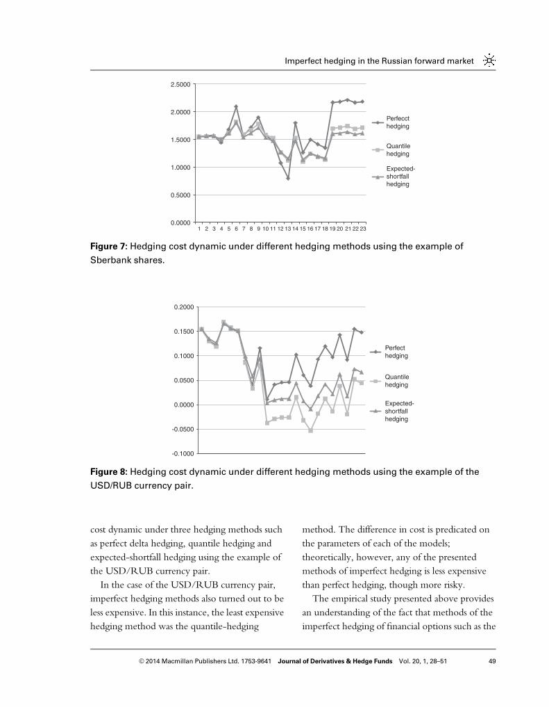
Thus, the tables presented above depicting theprocedures for different hedging methods lead tothe conclusion that imperfect hedging methodssuch as quantile hedging and expected-shortfallhedging make it possible to lower the cost of ahedging portfolio on the Russian forward marketby using controlled risk.Figure 7 illustrates the dynamic of hedging

cost under three hedging methods such asperfect delta hedging, quantile hedging andexpected-shortfall hedging using the exampleof Sberbank shares. The horizontal axis in thisfigure illustrates hedging day, and the verticalaxis – hedging portfolio cost.Thus, the least expensive hedging method

in this case turned out to be the expected-shortfall method at an anticipated-loss levelof 5 per cent. Slightly more expensive wasthe quantile-hedging method with a successprobability of 95 per cent. In this instance, perfecthedging was shown to be significantly moreexpensive, which confirms the theory of reducedhedging costs under the application of imperfecthedging methods. Figure 8 illustrates hedging92

.05

110.044

0.4658

0.0008

0.0007

0.2047

−0.0569

−5.2340

17.5696

18.8396

1.2701

91.52

120.04

0.3543

0.0002

0.0002

0.1569

−0.0478

−4.3702

13.2057

14.3609

1.1553

93.57

130.036

0.7465

0.0030

0.0028

0.3225

0.1656

15.4961

28.7065

30.1787

1.4722

92.55

140.032

0.5474

0.0003

0.0003

0.2424

−0.0801

−7.4146

21.3023

22.4352

1.1329

93.04

150.028

0.6543

0.0003

0.0003

0.2898

0.0474

4.4071

25.7171

26.9610

1.2440

92.91

160.024

0.6266

0.0001

0.0001

0.2782

−0.0116

−1.0743

24.6520

25.8491

1.1970

92.81

170.02

0.6020

0.0000

0.0000

0.2675

−0.0107

−0.9938

23.6671

24.8275

1.1604

94.48

180.016

0.9407

0.0003

0.0003

0.4170

0.1495

14.1260

37.8016

39.4002

1.5986

94.54

190.012

0.9659

0.0001

0.0001

0.4291

0.0121

1.1405

38.9557

40.5657

1.6100

94.63

200.008

0.9890

0.0000

0.0000

0.4396

0.0105

0.9914

39.9611

41.5957

1.6346

94.57

210.004

0.9990

0.0000

0.0000

0.4440

0.0044

0.4200

40.3955

41.9893

1.5938

94.64

220.000

1.0000

0.0000

0.0000

0.4444

0.0004

0.0418

40.4519

42.0622

1.6104



Table 8: Expected-shortfall hedging method using the example of the USD/RUB currency pair

Quote # T ΔС(K) ΔС(h) ΔCoN(h) ΔV Purchase Purchase cost Credit amount Value of theportfolio asset

Portfolio cost

30.1139 0 0.088 0.9964 0.0262 0.0260 0.4267 0.4267 12.8507 12.6960 12.8507 0.154730.0773 1 0.084 0.9862 0.0068 0.0068 0.4341 0.0074 0.2217 12.9223 13.0568 0.134530.0692 2 0.08 0.9790 0.0032 0.0032 0.4331 −0.0010 −0.0300 12.8970 13.0233 0.126330.1713 3 0.076 0.9993 0.0371 0.0369 0.4213 −0.0118 −0.3560 12.5456 12.7115 0.165930.159 4 0.072 0.9986 0.0191 0.0190 0.4321 0.0108 0.3252 12.8754 13.0316 0.156230.1575 5 0.068 0.9982 0.0119 0.0118 0.4364 0.0043 0.1288 13.0088 13.1597 0.150930.0496 6 0.064 0.9252 0.0001 0.0001 0.4112 −0.0252 −0.7573 12.2561 12.3553 0.099229.9598 7 0.06 0.5445 0.0000 0.0000 0.2420 −0.1691 −5.0675 7.1931 7.2509 0.057830.1231 8 0.056 0.9885 0.0004 0.0004 0.4391 0.1970 5.9351 13.1308 13.2256 0.094829.9251 9 0.052 0.2393 0.0000 0.0000 0.1064 −0.3327 −9.9557 3.1799 3.1830 0.003129.9966 10 0.048 0.5763 0.0000 0.0000 0.2562 0.1498 4.4932 7.6742 7.6838 0.009630.0161 11 0.044 0.6331 0.0000 0.0000 0.2814 0.0252 0.7566 8.4336 8.4454 0.011830.0277 12 0.04 0.6442 0.0000 0.0000 0.2863 0.0050 0.1488 8.5854 8.5974 0.012030.1513 13 0.036 0.9912 0.0000 0.0000 0.4406 0.1542 4.6504 13.2389 13.2832 0.044330.0782 14 0.032 0.8297 0.0000 0.0000 0.3688 −0.0718 −2.1594 11.0842 11.0916 0.007430.0451 15 0.028 0.5559 0.0000 0.0000 0.2471 −0.1217 −3.6557 7.4325 7.4237 −0.0088

30.1648 16 0.024 0.9938 0.0000 0.0000 0.4417 0.1946 5.8698 13.3050 13.3231 0.018130.2292 17 0.02 1.0000 0.0000 0.0000 0.4444 0.0028 0.0832 13.3931 13.4348 0.041730.195 18 0.016 0.9995 0.0000 0.0000 0.4442 −0.0002 −0.0065 13.3914 13.4131 0.021730.297 19 0.012 1.0000 0.0000 0.0000 0.4444 0.0002 0.0069 13.4032 13.4653 0.062230.2065 20 0.008 1.0000 0.0000 0.0000 0.4444 0.0000 −0.0001 13.4078 13.4250 0.017130.3431 21 0.004 1.0000 0.0000 0.0000 0.4444 0.0000 0.0001 13.4128 13.4858 0.073030.3399 22 0.000 1.0000 0.0000 0.0000 0.4444 0.0000 0.0000 13.4176 13.4844 0.0668

Nazarova

48

©2014Macmilla

nPublis

hers

Ltd.1753-9641

JournalofDeriv

ativ

es&

HedgeFunds

Vol.20,1,28–51

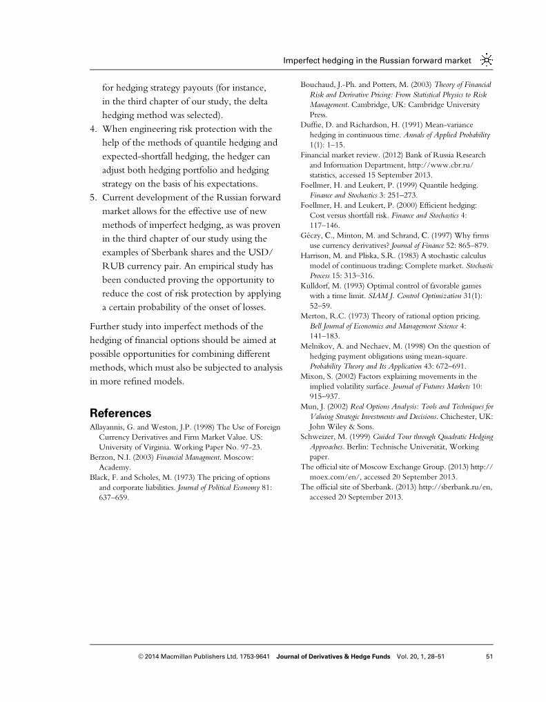
cost dynamic under three hedging methods suchas perfect delta hedging, quantile hedging andexpected-shortfall hedging using the example ofthe USD/RUB currency pair.In the case of the USD/RUB currency pair,

imperfect hedging methods also turned out to beless expensive. In this instance, the least expensivehedging method was the quantile-hedging

method. The difference in cost is predicated onthe parameters of each of the models;theoretically, however, any of the presentedmethods of imperfect hedging is less expensivethan perfect hedging, though more risky.The empirical study presented above provides

an understanding of the fact that methods of theimperfect hedging of financial options such as the

0.0000

0.5000

1.0000

1.5000

2.0000

2.5000

1 2 3 4 5 6 7 8 9 10 11 12 13 14 15 16 17 18 19 20 21 22 23

Perfecct hedging

Quantilehedging


Figure 7: Hedging cost dynamic under different hedging methods using the example of

Sberbank shares.

-0.1000

-0.0500

0.0000

0.0500

0.1000

0.1500

0.2000

Perfect hedging

Quantile hedging


Figure 8: Hedging cost dynamic under different hedging methods using the example of the

USD/RUB currency pair.



quantile-hedging method and the expected-shortfall hedging method are capable of beingintegrated into the concept of dynamic hedgingat a discrete point in time. Even the choice ofsuch a simple method as delta hedging within theBlack–Scholes model clearly demonstrates theopportunities presented by the aforementionedconcepts of imperfect hedging in terms ofreducing the cost of a hedging portfolio at acontrolled level of risk. With a sufficiently highlevel of confidence, we can assume that under theuse of refined models of dynamic hedging, theaccuracy of the results would be enhanced.

CONCLUSION

1. Analysis of methods based on the theory ofthe hedging of financial options has enabledthe compilation of a working classification ofthe main thrusts of foreign studies into themethods of the imperfect hedging of financialoptions. During the course of the study, it wasestablished that methods of the imperfecthedging of financial options represent a fun-damentally new approach to the managementof financial risks of positions stemming fromsuch derivative instruments as options. Thisapproach makes it possible to take intoaccount the expectations of the holder of aforward position, as well as his attitude towardrisk. Also taken into account are the nuancesof the hedger strategy when engineeringprotection against risk.

2. (a) In our study, we were able to demonstratethat methods of the imperfect hedging offinancial options reduce the cost of thehedging portfolio by virtue of possiblelosses.

(b) The set of successful hedging dependson forward position type, selected risk

measure, and parameters such as volatility,average growth rate and bank interestrate.That said, hedging strategy may be opti-mal under either one criterion (quantileor expected shortfall) or under both cri-teria at once – provided the satisfaction ofcertain conditions.

(c) The quantile-hedging method has certaindrawbacks. The greatest criticism is drawnby the fact that under its use, only theprobability of the onset of losses is takeninto account – not their amount. In thissense, in cases of the practical applicationof methods of imperfect hedging in orderto protect against financial risk, it is betterto use the expected-shortfall method,insofar as this method takes into accountboth the probability of possible losses aswell as their amount.

(d) It was discovered that as a rule, the cost ofhedging a forward position is not equal tothe total cost of its elements, insofar as theabove-mentioned examples establishedthat the additivity property is lacking frommethods of the imperfect hedging offinancial options such as quantile hedgingand expected-shortfall hedging.

3. In the course of the study, an algorithm wasconstructed for the implementation of hed-ging strategy according to methods ofthe imperfect hedging of financial options:Step 1. Identification of the structure ofsuccessful hedging set based on option typeand parameters such as volatility, averagegrowth rate and the bank interest rate.Step 2. Determination of hedging strategypayout within the hedging strategy set.Step 3. Selection of the method of replication

Nazarova


for hedging strategy payouts (for instance,in the third chapter of our study, the deltahedging method was selected).

4. When engineering risk protection with thehelp of the methods of quantile hedging andexpected-shortfall hedging, the hedger canadjust both hedging portfolio and hedgingstrategy on the basis of his expectations.

5. Current development of the Russian forwardmarket allows for the effective use of newmethods of imperfect hedging, as was provenin the third chapter of our study using theexamples of Sberbank shares and the USD/RUB currency pair. An empirical study hasbeen conducted proving the opportunity toreduce the cost of risk protection by applyinga certain probability of the onset of losses.

Further study into imperfect methods of thehedging of financial options should be aimed atpossible opportunities for combining differentmethods, which must also be subjected to analysisin more refined models.

ReferencesAllayannis, G. and Weston, J.P. (1998) The Use of Foreign

Currency Derivatives and Firm Market Value. US:University of Virginia. Working Paper No. 97-23.

Berzon, N.I. (2003) Financial Managment. Moscow:Academy.

Black, F. and Scholes, M. (1973) The pricing of optionsand corporate liabilities. Journal of Political Economy 81:637–659.

Bouchaud, J.-Ph. and Potters, M. (2003) Theory of FinancialRisk and Derivative Pricing: From Statistical Physics to RiskManagement. Cambridge, UK: Cambridge UniversityPress.

Duffie, D. and Richardson, H. (1991) Mean-variancehedging in continuous time. Annals of Applied Probability1(1): 1–15.

Financial market review. (2012) Bank of Russia Researchand Information Department, http://www.cbr.ru/statistics, accessed 15 September 2013.

Foellmer, H. and Leukert, P. (1999) Quantile hedging.Finance and Stochastics 3: 251–273.

Foellmer, H. and Leukert, P. (2000) Efficient hedging:Cost versus shortfall risk. Finance and Stochastics 4:117–146.

Géczy, С., Minton, M. and Schrand, С. (1997) Why firmsuse currency derivatives? Journal of Finance 52: 865–879.

Harrison, M. and Pliska, S.R. (1983) A stochastic calculusmodel of continuous trading: Complete market. StochasticProcess 15: 313–316.

Kulldorf, M. (1993) Optimal control of favorable gameswith a time limit. SIAM J. Control Optimization 31(1):52–59.

Merton, R.C. (1973) Theory of rational option pricing.Bell Journal of Economics and Management Science 4:141–183.

Melnikov, A. and Nechaev, M. (1998) On the question ofhedging payment obligations using mean-square.Probability Theory and Its Application 43: 672–691.

Mixon, S. (2002) Factors explaining movements in theimplied volatility surface. Journal of Futures Markets 10:915–937.

Mun, J. (2002) Real Options Analysis: Tools and Techniques forValuing Strategic Investments and Decisions. Chichester, UK:John Wiley & Sons.

Schweizer, M. (1999) Guided Tour through Quadratic HedgingApproaches. Berlin: Technische Universität, Workingpaper.

The official site of Moscow Exchange Group. (2013) http://moex.com/en/, accessed 20 September 2013.

The official site of Sberbank. (2013) http://sberbank.ru/en,accessed 20 September 2013.



http://www.cbr.ru/statistics

http://www.cbr.ru/statistics

http://moex.com/en/

http://moex.com/en/

http://sberbank.ru/en

Documents

Evaluation of the effectiveness of methods of the ... · The classical solution to ... while the question of the economic effectiveness ... that the use of currency-based derivatives