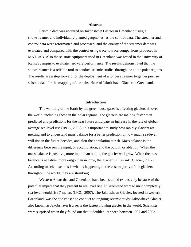
Evaluation of Seismic Data acquired with a Streamer on the Jakobshavn Glacier, Greenland

Edil A. Sepulveda Carlo, Jose Velez, Anthony Hoch, and George Tsoflias

University of Kansas 2335 Irving Hill Road

Lawrence, KS 66045-7612 http://cresis.ku.edu

Technical Report CReSIS TR 130

July 30, 2007

This work was supported by a grant from the

National Science Foundation (#ANT-0424589).

Abstract

Seismic data was acquired on Jakobshavn Glacier in Greenland using a

snowstreamer and individually-planted geophones, as the control data. The streamer and

control data were reformatted and processed, and the quality of the streamer data was

evaluated and compared with the control using trace to trace comparisons produced in

MATLAB. Also the seismic equipment used in Greenland was tested in the University of

Kansas campus to evaluate hardware performance. The results demonstrated that the

snowstreamer is a reliable tool to conduct seismic studies through ice at the polar regions.

The results are a step forward for the deployment of a longer streamer to gather precise

seismic data for the mapping of the subsurface of Jakobshavn Glacier in Greenland.

Introduction

The warming of the Earth by the greenhouse gases is affecting glaciers all over

the world, including those in the polar regions. The glaciers are melting faster than

predicted and predictions for the near future anticipate an increase in the rate of global

average sea-level rise (IPCC, 2007). It is important to study how rapidly glaciers are

melting and to understand mass balance for a better prediction of how much sea-level

will rise in the future decades, and alert the population at risk. Mass balance is the

difference between the input, or accumulation, and the output, or ablation. When the

mass balance is positive, more input than output, the glacier will grow. When the mass

balance is negative, more outgo than income, the glacier will shrink (Glacier, 2007).

According to scientists this is what is happening to the vast majority of the glaciers

throughout the world, they are shrinking.

Western Antarctica and Greenland have been studied extensively because of the

potential impact that they present to sea level rise. If Greenland were to melt completely,

sea-level would rise 7 meters (IPCC, 2007). The Jakobshavn Glacier, located in western

Greenland, was the site chosen to conduct an ongoing seismic study. Jakobshavn Glacier,

also known as Jakobshavn Isbrae, is the fastest flowing glacier in the world. Scientists

were surprised when they found out that it doubled its speed between 1997 and 2003

2

(http://www.nasa.gov/vision/earth/lookingatearth/jakobshavn.html). The motion of this

glacier is estimated at 40 meters per day or almost 15 kilometers per year (Maas, 2006).

Seismic imaging is a suitable method to identify ice thickness and the layers

above and below the base of the ice. With this information, glaciologists can then

understand the movement and melting rate of this glacier, and many others in Greenland

and Antarctica. For this reason, geophysicists at CReSIS, the Center for Remote Sensing

on Ice Sheets, are researching different methods to efficiently acquire seismic data in the

polar regions. Conventional seismic methods, as individually-planted geophones, are

time-consuming and labor intensive. A snowstreamer, an array of geophones towed over

ice, has been developed at CReSIS for the acquisition of seismic data at Jakobshavn

Glacier, in Greenland.

Background

Geophysics is the measurement of contrasts in the physical properties of materials

beneath the surface of the Earth and the attempt to deduce the nature and distribution of

the materials responsible for these observations. Variations in elastic moduli and density

cause seismic waves to travel at different speeds through different materials. By timing

the arrivals of these waves at surface observation points, we can deduce a great deal

about the nature and distribution of subsurface bodies (Burger, 2006) like, in this case,

the recognition of the internal layers of the ice, the bedrock, and the internal layers of the

bed.

Seismic streamers were originally designed for marine studies, but they have been

proven to work reasonably well in other environments on land and snow. What worries

geophysicists about the use of streamers for seismic studies in general, are the quality of

the geophone coupling to the ground and the level of ambient noise that they can display

(Eiken, 1989). These problems are the ones that haven’t allowed streamers to become

common tools in recording seismic data in polar environments.

3

Objectives

The objective of this project is to evaluate the quality of streamer data acquired in

May 2007 on Jakobshavn Glacier in Greenland. To accomplish that we:

• Process the seismic data using commercially available software and by writing

MATLAB code.

• Determine whether streamer data is comparable to the control data gathered using

individually-planted geophones.

• Determine how much wind noise affects the quality of the data acquired by the

snowstreamer.

• Determine the best streamer setup for optimum data quality.

• Interpret the data and identify the bedrock and other internal layers of the ice and

bedrock.

• Evaluate if the snowstreamer can be used to identify the bed, internal ice layers

and other geologic features beneath the bed.

• Test the seismic equipment used in Greenland to evaluate hardware performance.

What is a streamer?

A streamer is a set of geophones joint together by cables used to record seismic

data. It is a useful tool because it can facilitate the gathering of seismic data. The streamer

constructed for the seismic research on Jakobshavn Glacier in Greenland consisted of a

set of geophones mounted on steel and aluminum base plates joint together with a fire

hose. It was assembled by CReSIS Graduate Research Assistants, Anthony Hoch,

Geophysics Graduate Student, and Chris Gifford, robotics specialist, at the University of

Kansas. The weight of the streamer was approximately 200 pounds. Streamer cost was

around $2,000.

The setup of the streamer used in Greenland consisted of 24 conventional

geophones mounted on eight plates, four aluminum and four steel. The plates were

spaced 1.5 meters from each other, for a total streamer length of 12 meters. The

streamer’s geometry consisted of 8 vertical and 16 horizontal (SV and SH) geophones.

Each plate had 1 vertical and 2 horizontal geophones. They were positioned in

4

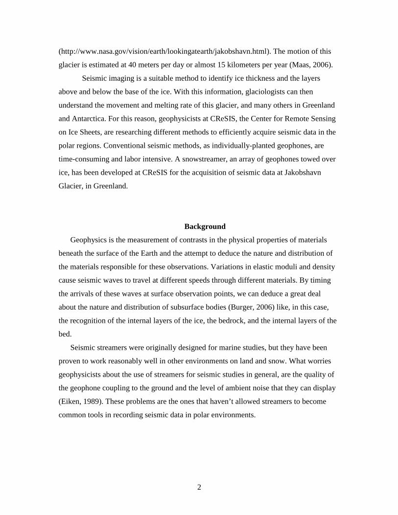
conventional orientation and Galperin orientation, another type of configuration where

geophones are positioned at different angles. Figure 1 shows the configuration of the

geophones on the snowstreamer deployed on Jakobshavn Glacier.

Figure 1 – Snowstreamer deployed on Jakobshavn Glacier, Greenland (left) and geophone’s

configuration on the streamer (right)

Methodology

I. Data Acquisition

George Tsoflias and a group of scientists from Pennsylvania State University

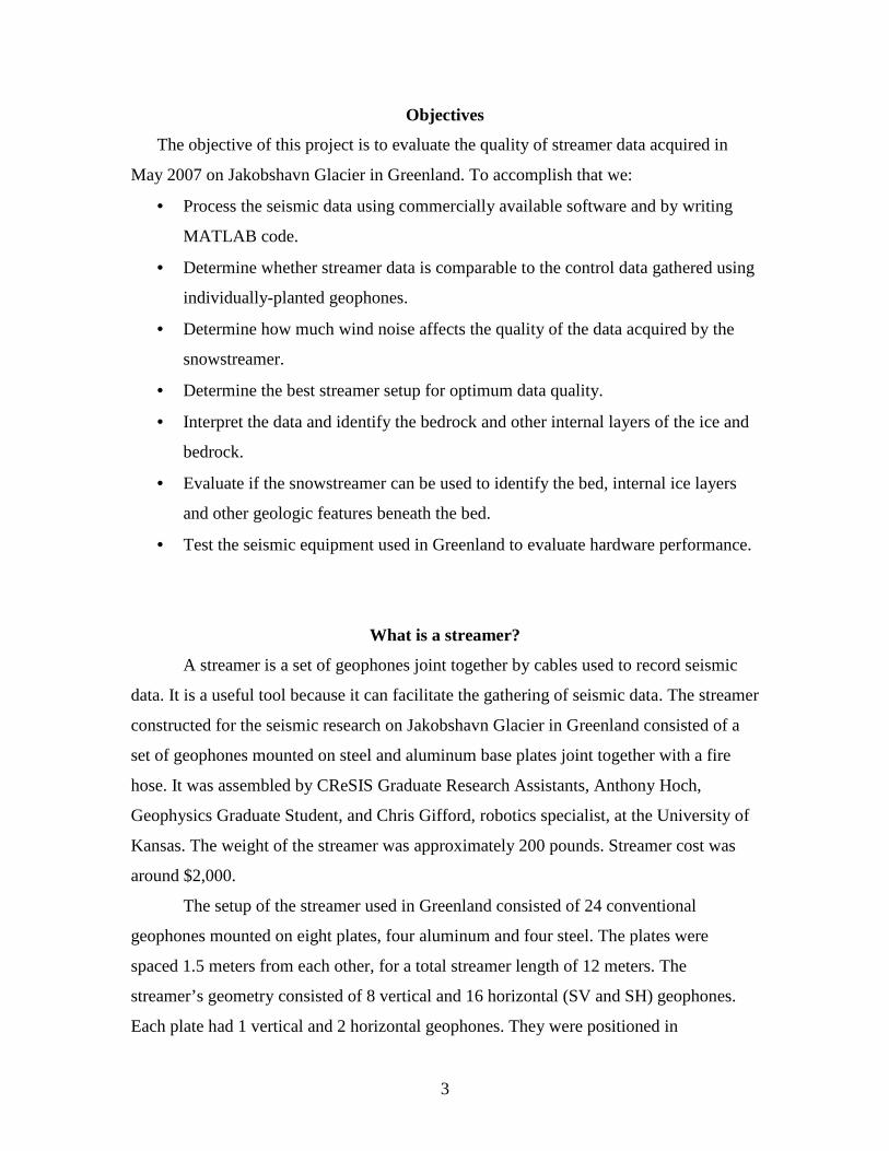
acquired seismic data on the Jakobshavn Glacier in May 2007. The snowstreamer

consisted of 24 geophones mounted on eight plates, meanwhile the control line, was

composed of 24 individually-planted geophones. The snowstreamer and the individual

geophones, or control line, were placed next to each other, as figure 2 shows.

Conventional

Galperin

5

Figure 2 – Snowstreamer next to the control line

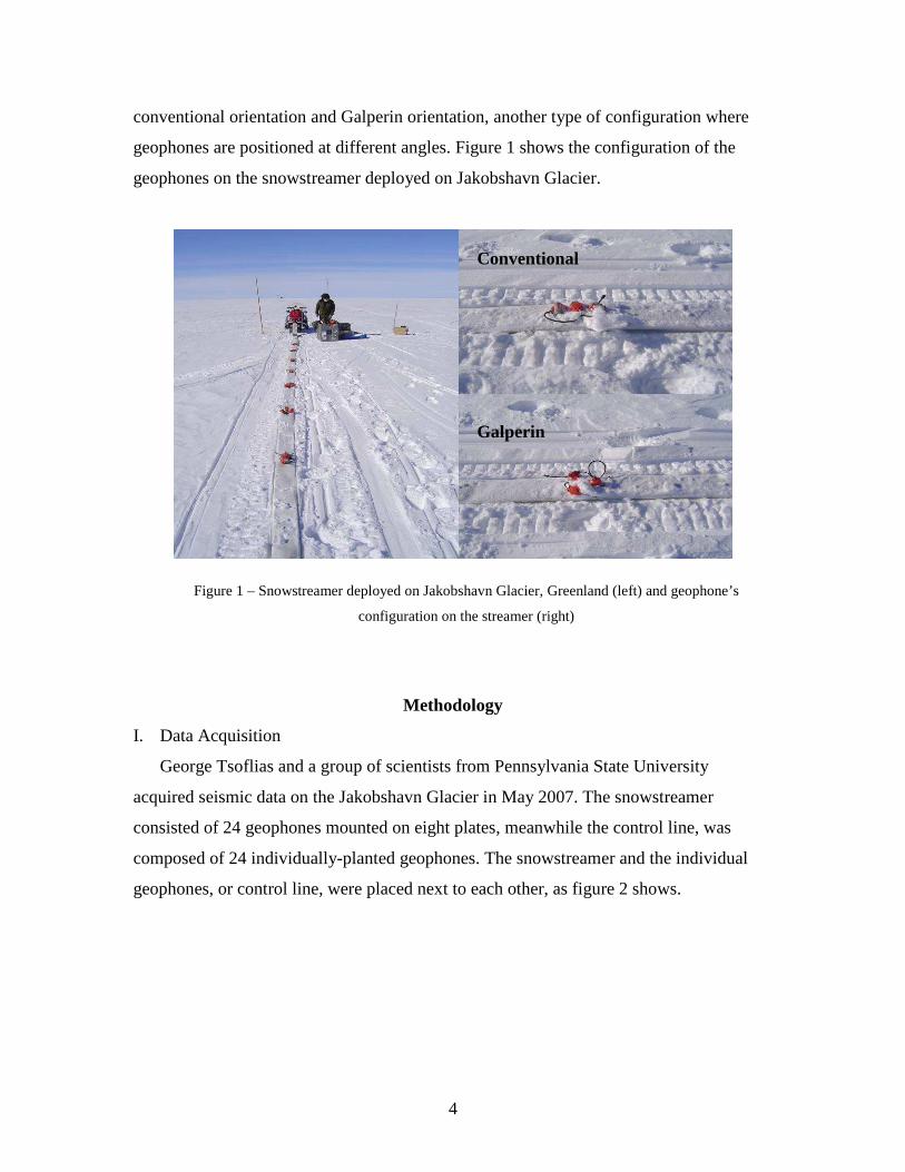
The source used to produce the sound waves was 0.5 kilograms of explosives

placed 10 meters below the surface. The source was advanced at 160 meters long

increments from the snowstreamer. Two lines were acquired for the study, named line 34

and line 51-52, the main line. Line 34 will not be used for the analysis because it didn’t

include the control line. Line 34 was used to test deployment of the snowstreamer in the

field. Line 51-52 consisted of 22 shots, or sources, but only 14 shots were used for the

analysis, because the first 8 shots didn’t include control line data due to malfunctioning

instrumentation.

II. Data Processing

Processing of the seismic data employed MATLAB and SPW. MATLAB is a high-

performance high level software language for technical computing. SPW, or Seismic

Processing Workshop, is a commercially available interactive seismic data processing

software (http://www.parallelgeo.com/products/productstxt.html).

The first step is to reformat the raw data that came from Greenland, changing it from

SEG2 to SEG-Y format, using the seismic program SPW I/O Utility. Using MATLAB, a

script was written to process the data and plot it in three different graph series. The script

used to produce the trace to trace comparison of the streamer and control data is included

at the appendix section.

6

III. Data Interpretation

The graphs and figures created after processing the raw data and inputting the

geometry and topography of the study area will be used for the interpretation of the

seismic data. The figures will include magnitude and frequency plots, a db graph, and a

shot gather image. The magnitude, frequency series and the dB graph were generated in

MATLAB and were used for the trace to trace comparison between the streamer and

control data. Meanwhile receiver gathers were generated in the seismic program SPW

SeisViewer, for a broader perspective of the data gathered by each streamer and control

channel. The figures will help us identify the bedrock reflection, the wave velocity, and

features or layers in the ice and beneath the bedrock.

IV. Evaluating the seismic instrumentation

On July 10, 2007 we tested in Lawrence, Kansas the seismic instrumentation used

in Greenland, to test if the differences in magnitude of the sound waves recorded by the

snowstreamer in Greenland were due to hardware problems. The site of the study was the

west campus of the University of Kansas (KU). The streamer geophones were

individually planted in a line next to the geophones of the control line, as seen in figure 3.

Figure 3 – Seismic study on west campus of KU on July 10, 2007

7

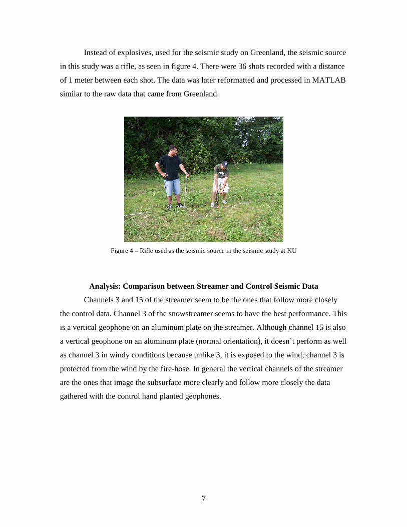
Instead of explosives, used for the seismic study on Greenland, the seismic source

in this study was a rifle, as seen in figure 4. There were 36 shots recorded with a distance

of 1 meter between each shot. The data was later reformatted and processed in MATLAB

similar to the raw data that came from Greenland.

Figure 4 – Rifle used as the seismic source in the seismic study at KU

Analysis: Comparison between Streamer and Control Seismic Data

Channels 3 and 15 of the streamer seem to be the ones that follow more closely

the control data. Channel 3 of the snowstreamer seems to have the best performance. This

is a vertical geophone on an aluminum plate on the streamer. Although channel 15 is also

a vertical geophone on an aluminum plate (normal orientation), it doesn’t perform as well

as channel 3 in windy conditions because unlike 3, it is exposed to the wind; channel 3 is

protected from the wind by the fire-hose. In general the vertical channels of the streamer

are the ones that image the subsurface more clearly and follow more closely the data

gathered with the control hand planted geophones.

8

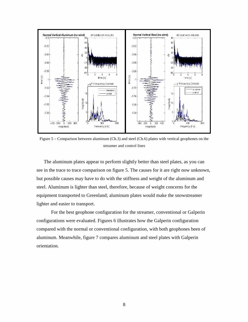
Figure 5 – Comparison between aluminum (Ch.3) and steel (Ch.6) plates with vertical geophones on the

streamer and control lines

The aluminum plates appear to perform slightly better than steel plates, as you can

see in the trace to trace comparison on figure 5. The causes for it are right now unknown,

but possible causes may have to do with the stiffness and weight of the aluminum and

steel. Aluminum is lighter than steel, therefore, because of weight concerns for the

equipment transported to Greenland; aluminum plates would make the snowstreamer

lighter and easier to transport.

For the best geophone configuration for the streamer, conventional or Galperin

configurations were evaluated. Figures 6 illustrates how the Galperin configuration

compared with the normal or conventional configuration, with both geophones been of

aluminum. Meanwhile, figure 7 compares aluminum and steel plates with Galperin

orientation.

9

Figure 6 – Comparison between normal orientation (Ch.3) and Galperin vertical orientation (Ch. 21)

Figure 7 – Comparison between channels 21 (left) and 24 (right) of the streamer

10

The vertical geophones on normal or conventional orientation appear less

sensitive to wind noise than the Galperin vertical channels. Galperin orientated

geophones were most sensitive to the wind noise than conventional vertical geophones.

For the horizontal channels, in particular, the SV channel, the Galperin geophone

performs as well as the conventional geophone, as seen in figure 8.

Figure 8 – Comparison between vertical (Ch.3) and SV (Ch.8) components of the streamer and control data

11

Figure 9 – Comparison between vertical (Ch.3) and horizontal (Ch.1) components of the streamer and

control data

The vertical component recordings were superior to horizontal component data, as

seen in figures 8 and 9. This appears very clearly in the data interpreted. The streamer

channels with horizontal orientations always show a lot of wind noise in the data. SH

component seems to not be an option. It performs only well to some extent under no wind

conditions, and with just a little wind the data becomes noisy. SV component can be an

option when the wind conditions are calm and the sensor is preferably Galperin.

The wind has a negative effect on the data gathered by the streamer. The individually-

planted geophones, or control, also are negatively affected by the wind. It brings higher

than normal noise to the data being gathered. The wind increases the magnitude or

amplitude of the seismic wave data recorded by the streamer and also the control. This

data that is later view and interpret through MATLAB, shows irregular magnitudes

caused by the wind, which impede an accurate identification of the bed or well as

interpretation of the different internal layers of the ice and bed. This is illustrated on the

trace to trace comparisons of streamer and control data in figure 10.

12

Figure 10 – Aluminum plates under different wind conditions

Results

The results of the comparison between streamer and control data illustrate that when

there is no wind the streamer data shows more clearly the bedrock reflection than the

control data. The magnitude of the seismic waves in the streamer data is higher than the

one from the control data, facilitating the identification of the bedrock at approximately 1

second. Even in conditions when the wind is strong, 10+ knots, the streamer data shows

13

the bedrock reflection at approximately 1 second, clearer than the control data, in some

cases. This depends a great deal on the direction of the geophone, if it is vertical or

horizontal.

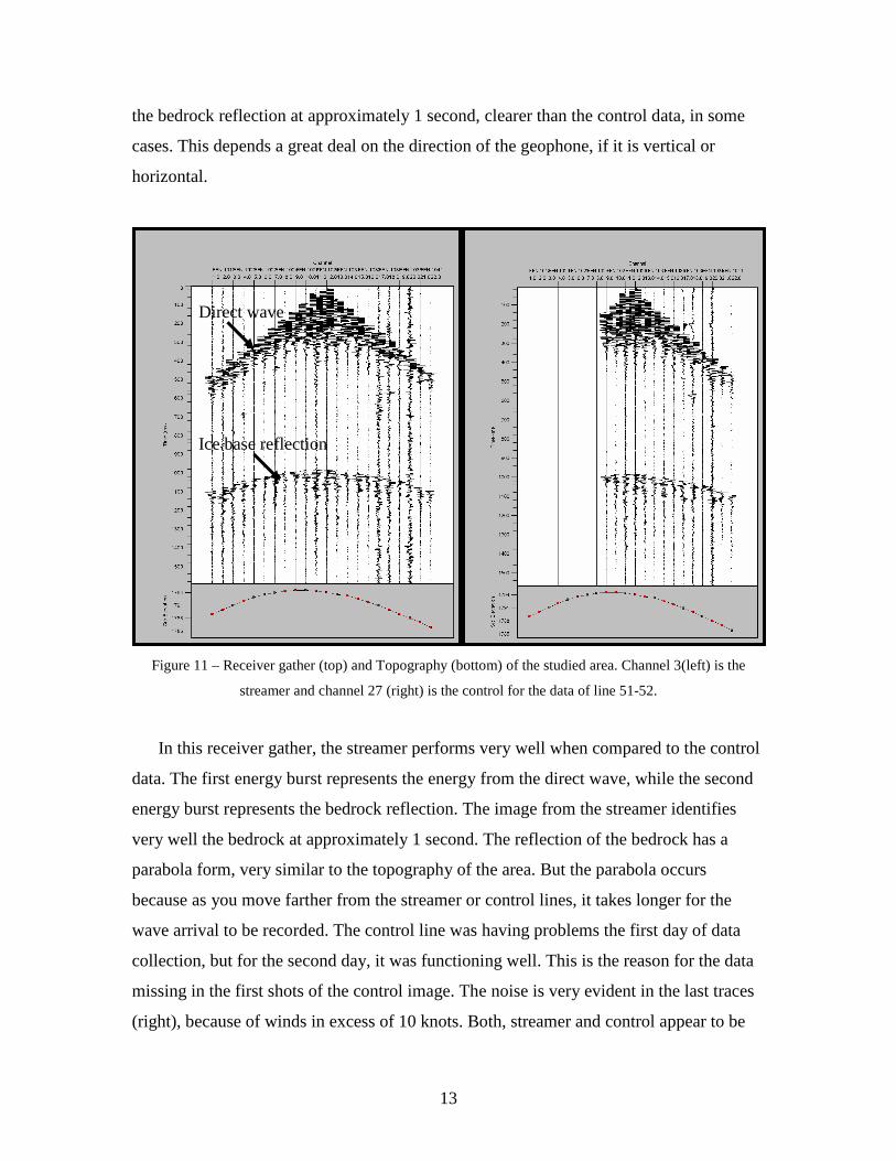
Figure 11 – Receiver gather (top) and Topography (bottom) of the studied area. Channel 3(left) is the

streamer and channel 27 (right) is the control for the data of line 51-52.

In this receiver gather, the streamer performs very well when compared to the control

data. The first energy burst represents the energy from the direct wave, while the second

energy burst represents the bedrock reflection. The image from the streamer identifies

very well the bedrock at approximately 1 second. The reflection of the bedrock has a

parabola form, very similar to the topography of the area. But the parabola occurs

because as you move farther from the streamer or control lines, it takes longer for the

wave arrival to be recorded. The control line was having problems the first day of data

collection, but for the second day, it was functioning well. This is the reason for the data

missing in the first shots of the control image. The noise is very evident in the last traces

(right), because of winds in excess of 10 knots. Both, streamer and control appear to be

Direct wave

Ice base reflection

14

affected by the wind noise. Multi-fold stacking, adding multiple channels to form a

simple trace, can improve the signal to noise ratio.

Figure 12 – Test of the seismic equipment used in Greenland (Seismic study at KU)

The seismic hardware test study conducted at KU showed excellent agreement

between the magnitude of the streamer and control seismic instrumentation, as seen on

figure 12. This means that the streamer data from Greenland compare rather well with the

individually-planted geophones, or control, and that no major hardware problems

occurred with the seismic equipment.

Conclusions and Recommendations

The interpretation and analysis from the data gathered and processed concludes

that this particular streamer constructed by scientists at CReSIS is, in fact, a reliable tool

to conduct seismic studies through ice at the polar regions. When there is no wind the

streamer performs very well, even better than the control handplants. When the wind

starts to pick up, less than 5 knots, the streamer continues to be a reliable tool to identify

the bed and the other internal layers of the ice and the bed. When the conditions are

15

windy, 10 or more knots, the streamer is certainly affected, but the bed can be identified

in some cases, depending on the streamer set up. At these windy conditions even the

control data is affect to a great extent. It also has to be considered that the streamer is

more exposed to the wind that the control line, whose geophones are buried in the snow.

From the analysis we also can conclude that the best streamer setup is

conventional vertical geophones on aluminum plates. The steel plates didn’t perform as

well as the aluminum plates. The conventional or normal orientation was far better than

the Galperin geophone configuration.

The vertical component is the ideal set up for the streamer; horizontal components

do not detect P-waves as well as vertical ones. The recommendations are to not to use the

horizontal component (SH) in the streamer. The SV component needs further revision to

determine if it can be a reliable alternative for the seismic methods on glacier research.

The Galperin orientation on the SV channels performs rather well, but only when there is

no wind. At the moment, the SV and SH components of the streamer aren’t expected to

be used for further research.

From the interpretation of the figures we can conclude that the streamer can be

used to identify the bedrock, and even also other internal ice layers and geologic features

beneath the bed. We concluded that there was no hardware malfunction in the seismic

equipment used in Greenland; therefore, the streamer performs similarly or even better

than the individually-planted geophones, or control line. The results are a step forward

for the deployment of a longer streamer to gather precise seismic data for the mapping of

the subsurface of Jakobshavn Glacier in Greenland.

Future Work

There is a great deal of work scheduled for the use of the snowstreamer in seismic

studies through ice. They include:

• Construct a longer snowstreamer, 500 meters or 1 kilometer long. The setup of

the new streamer would consist of aluminum plates with conventional vertical

geophones.

16

• For May 2008 another expedition to Greenland is planed to collect seismic data

from Jakobshavn Glacier using the newly constructed snowstreamer.

• 2-D and 3-D mapping of the subsurface of Jakobshavn Glacier will be possible

using the seismic data gathered by the snowstreamer.

Acknowledgements

We would like to thank CReSIS and the NSF for the opportunity given to conduct

this research work and the help provided to achieve our work and presenting it in this

technical report.

References

Burger, H.R., Sheehan A.F., & Jones C.H., 2006: Introduction to Applied

Geophysics: Exploring the Shallow Subsurface. Rev. ed of: Englewood Cliffs, N.J.:

Prentice Hall, © 1992.

Eiken, O., Degutsch, M., Ritse, P., & Rod, K., 1989: Snowstreamer: an efficient

tool in seismic acquisition. First Break, Vol.7, Issue 9, 374-378.

Glacier. (2007). In Encyclopedia Britannica. Retrieved July 2, 2007, from

Encyclopedia Britannica Online: http://www.britannica.com/eb/article-65670

IPCC, 2007: Summary for Policymakers. In: Climate Change 2007: The Physical

Science Basis. Contribution of Working Group I to the Fourth Assessment Report of the

Intergovernamental Panel on Climate Change [Solomon, S., D. Qin, M. Manning, Z.

Chen, M. Marquis, K.B. Averyt, M. Tignor and H.L. Miller (eds.)]. Cambridge

University Press, Cambridge, United Kingdom and New York, NY, USA.

Maas, H.R., Dietrich, R., Schwalbe, E., Babler, M, & Westfeld, P., 2006: Analysis

of the Motion Behaviour of Jakobshavn Isbrae Glacier in Greenland by Monocular

Image Sequence Analysis. IAPRS Volume XXXVI.

http://www.nasa.gov/vision/earth/lookingatearth/jakobshavn.html

http://www.parallelgeo.com/products/productstxt.html

17

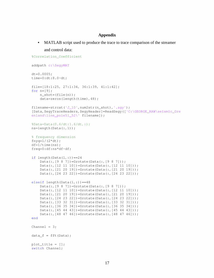
Appendix

• MATLAB script used to produce the trace to trace comparison of the streamer

and control data:

%Correlation_Coefficient addpath c:\SegyMAT dt=0.0005; time=0:dt:8.0-dt; file=[18:1:25, 27:1:34, 36:1:39, 41:1:42]; for n=[9]; n_shot=(file(n)); data=zeros(length(time),48); filename=strcat( 'J_10' ,num2str(n_shot), '.sgy' ); [Data,SegyTraceHeaders,SegyHeader]=ReadSegy([ 'C:\GEORGE_RAW\seismic_Greenland\line_pole51_52\' filename]); %Data=Data(0.6/dt:1.6/dt,:); ns=length(Data(:,1)); % frequency dimension fnyq=1/(2*dt); df=1/time(ns); freq=0:df:ns*df-df; if length(Data(1,:))==24 Data(:,[9 8 7])=Grotate(Data(:,[9 8 7])); Data(:,[12 11 10])=Grotate(Data(:,[12 11 10])); Data(:,[21 20 19])=Grotate(Data(:,[21 20 19])); Data(:,[24 23 22])=Grotate(Data(:,[24 23 22])); elseif length(Data(1,:))==48 Data(:,[9 8 7])=Grotate(Data(:,[9 8 7])); Data(:,[12 11 10])=Grotate(Data(:,[12 11 10])); Data(:,[21 20 19])=Grotate(Data(:,[21 20 19])); Data(:,[24 23 22])=Grotate(Data(:,[24 23 22])); Data(:,[33 32 31])=Grotate(Data(:,[33 32 31])); Data(:,[36 35 34])=Grotate(Data(:,[36 35 34])); Data(:,[45 44 43])=Grotate(Data(:,[45 44 43])); Data(:,[48 47 46])=Grotate(Data(:,[48 47 46])); end Channel = 3; data_f = fft(Data); plot_title = []; switch Channel;

18

case 3, plot_title = [plot_title 'Normal Vertical Aluminum' ]; case 6, plot_title = [plot_title 'Normal Vertical Steel' ]; case 9, plot_title = [plot_title 'Galperin Vertical Aluminum' ]; case 12, plot_title = [plot_title 'Galperin Vertical Steel' ]; case 15, plot_title = [plot_title 'Normal Vertical Aluminum' ]; case 18, plot_title = [plot_title 'Normal Vertical Steel' ]; case 21, plot_title = [plot_title 'Galperin Vertical Aluminum' ]; case 24, plot_title = [plot_title 'Galperin Vertical Steel' ]; end switch n; case 9, plot_title = [plot_title ' (no wind)' ]; case 10, plot_title = [plot_title ' (no wind)' ]; case 11, plot_title = [plot_title ' (no wind)' ]; case 12, plot_title = [plot_title ' (no wind)' ]; case 13, plot_title = [plot_title ' (no wind)' ]; case 14, plot_title = [plot_title ' (wind 1-2 knots)' ]; case 15, plot_title = [plot_title ' (wind 2-3 knots)' ]; case 16, plot_title = [plot_title ' (wind 5+ knots)' ]; case 17, plot_title = [plot_title ' (wind 10 knots)' ]; case 18, plot_title = [plot_title ' (wind 10 knots)' ]; case 19, plot_title = [plot_title ' (wind 10 knots)' ]; case 20, plot_title = [plot_title ' (wind 10 knots)' ]; case 21, plot_title = [plot_title ' (wind 5-10 knots)' ]; case 22, plot_title = [plot_title ' (wind 5 knots)' ]; end time=time(1:(length(Data(:,1)))); figure; subplot(1,2,1); plot(Data(:,Channel),-time, 'b' ,Data(:,Channel+24),-time, 'k' ); title(plot_title); xlabel( 'magnitude' ); ylabel( 'time (s)' ); axis([-200 200 -1.1 -0.9]); subplot(2,2,4); plot(freq,abs(data_f(:,Channel)), 'b' ,freq,abs(data_f(:,Channel+24)), 'k'); title( 'Frequency Domain' ); xlabel( 'frequency (Hz)' ); ylabel( 'magnitude' ); axis([0 fnyq 0 max(abs(data_f(:,Channel)))]); legend( 'streamer' , 'control' ); mag = 20.*log10(abs(Hilbert(Data)).*(1.6985e-4).*10 00); %dBm (dB relative to milivolts) subplot(2,2,2); plot(time, mag(:,Channel), 'b' ,time, mag(:,Channel+24), 'k' ); title( 'dB relative to milivolts' ); xlabel( 'time (s)' ); ylabel( 'db' ); end