Click to edit Master title style

1

Hani S. Mahmassani Maryland Transportation InitiativeMaryland Transportation Initiative

University of MarylandUniversity of Maryland

Evaluation of Road Pricing Schemes

Transport Forum 2006 The World Bank, Washington, D.C.

March 29, 2006

??

Growing Congestion….

Two Key Motivating Phenomena….

Highway Authorities….

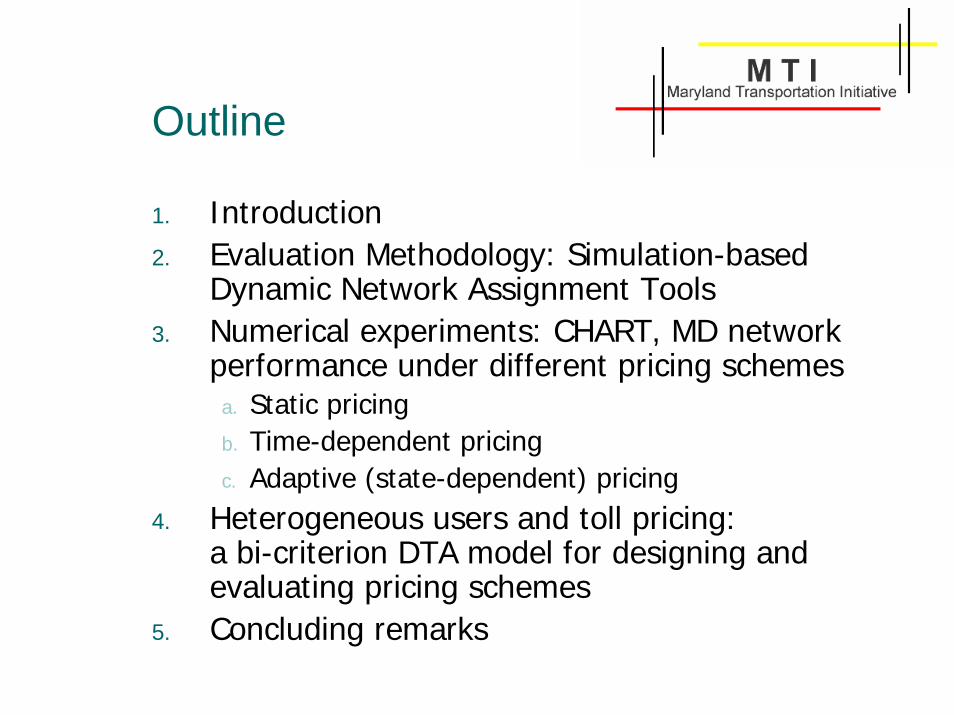
Outline

1. Introduction 2. Evaluation Methodology: Simulation-based

Dynamic Network Assignment Tools3. Numerical experiments: CHART, MD network

performance under different pricing schemesa. Static pricingb. Time-dependent pricingc. Adaptive (state-dependent) pricing

4. Heterogeneous users and toll pricing: a bi-criterion DTA model for designing and evaluating pricing schemes

5. Concluding remarks

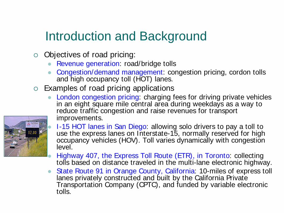
Introduction and BackgroundObjectives of road pricing:

Revenue generation: road/bridge tollsCongestion/demand management: congestion pricing, cordon tolls and high occupancy toll (HOT) lanes.

Examples of road pricing applicationsLondon congestion pricing: charging fees for driving private vehicles in an eight square mile central area during weekdays as a way toreduce traffic congestion and raise revenues for transport improvements.I-15 HOT lanes in San Diego: allowing solo drivers to pay a toll to use the express lanes on Interstate-15, normally reserved for high occupancy vehicles (HOV). Toll varies dynamically with congestion level.Highway 407, the Express Toll Route (ETR), in Toronto: collecting tolls based on distance traveled in the multi-lane electronic highway.State Route 91 in Orange County, California: 10-miles of express toll lanes privately constructed and built by the California Private Transportation Company (CPTC), and funded by variable electronictolls.

Rationale for Congestion Pricing

1. Market-clearing prices: charge whatever it takes to achieve desired service levels – use prices instead of wasted time/queues to rationalize use of transport infrastructure; efficiency argument.

2. To induce more efficient use of transport infrastructure–Network Equilibrium Theory: Use pricing to induce (Time-

minimizing) system optimal (SO) flow pattern instead of inefficient user equilibrium (UE) attained without pricing.

First-best pricing: Charge users marginal cost (imposed on system) on all network links;

Second-best pricing: Impose tolls only on selected links (usually for practical reasons)

Congestion Pricing as Demand Management Tool1. Pricing increasingly viewed as one instrument along with

two main other controls for integrated transportation system management:

1. Traffic controls: ramp metering, signal coordination2. Information Supply: advanced traveler information systems,

parking information systems, variable message signs (VMS)…

2. In real-time: with improved sensing and information technologies, can determine prices, traffic controls and information strategies adaptively, online, based on current and anticipated state of the system

HOT LANES

Single Occupant Vehicles allowed to use HOV lanes for a toll

Toll rates vary based on traffic conditions or time of day so as to maintain high level of service on managed lane

Facilitated by AVI and automatic toll collection

Hot lanes will only be considered with the addition of a lane to the Beltway. No general purpose lanes will be converted to HOT lanes.

Electronic Payment Services throughRFID Tags: m-commerce

Return to list

e-Drive

Drive-thru fast food, gasoline,car wash, etc

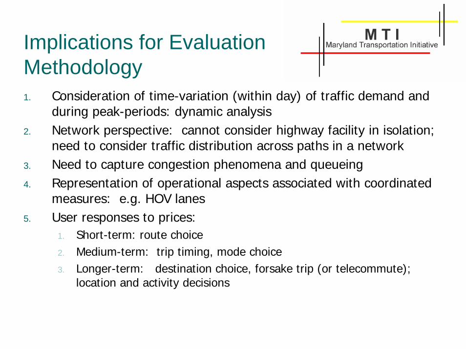
Implications for Evaluation Methodology1. Consideration of time-variation (within day) of traffic demand and

during peak-periods: dynamic analysis2. Network perspective: cannot consider highway facility in isolation;

need to consider traffic distribution across paths in a network3. Need to capture congestion phenomena and queueing4. Representation of operational aspects associated with coordinated

measures: e.g. HOV lanes5. User responses to prices:

1. Short-term: route choice2. Medium-term: trip timing, mode choice3. Longer-term: destination choice, forsake trip (or telecommute);

location and activity decisions

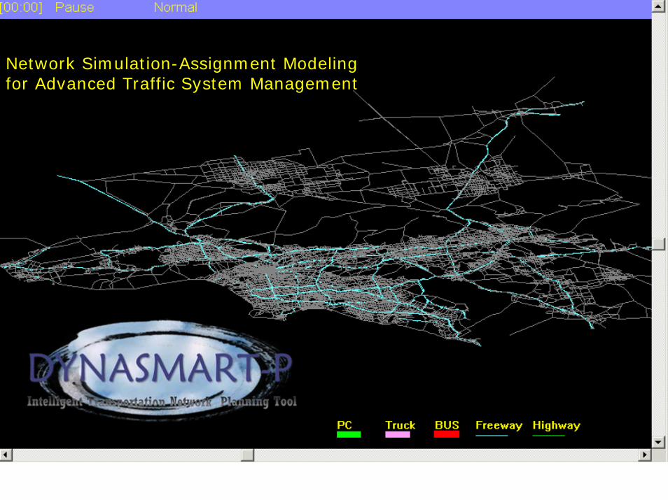
Network Simulation-Assignment Modeling for Advanced Traffic System Management

Road Pricing Applications with DYNASMART-P

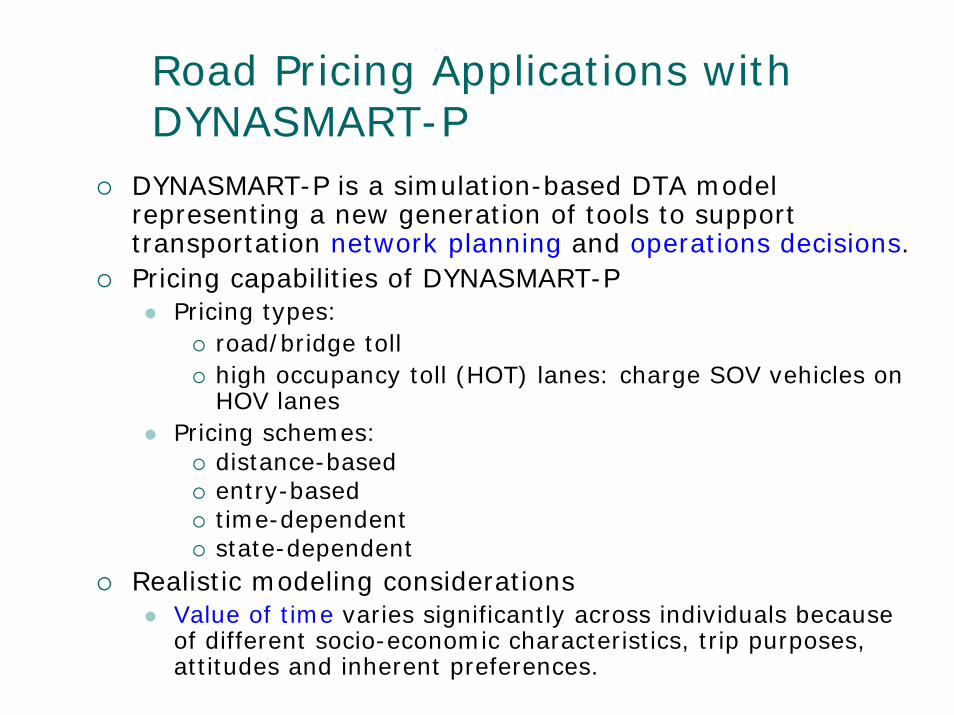
DYNASMART-P is a simulation-based DTA model representing a new generation of tools to support transportation network planning and operations decisions. Pricing capabilities of DYNASMART-P

Pricing types: road/bridge toll high occupancy toll (HOT) lanes: charge SOV vehicles on HOV lanes

Pricing schemes: distance-based entry-based time-dependentstate-dependent

Realistic modeling considerationsValue of time varies significantly across individuals because of different socio-economic characteristics, trip purposes, attitudes and inherent preferences.

Road Pricing Applications with DYNASMART-P

Input pricing schemes

Input pricing schemes

Road Pricing Applications with DYNASMART-P

Display of toll links in GUI

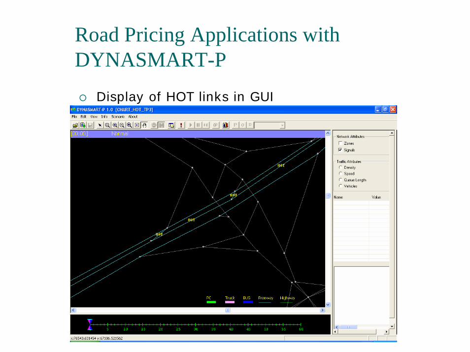
Road Pricing Applications with DYNASMART-P

Display of HOT links in GUI

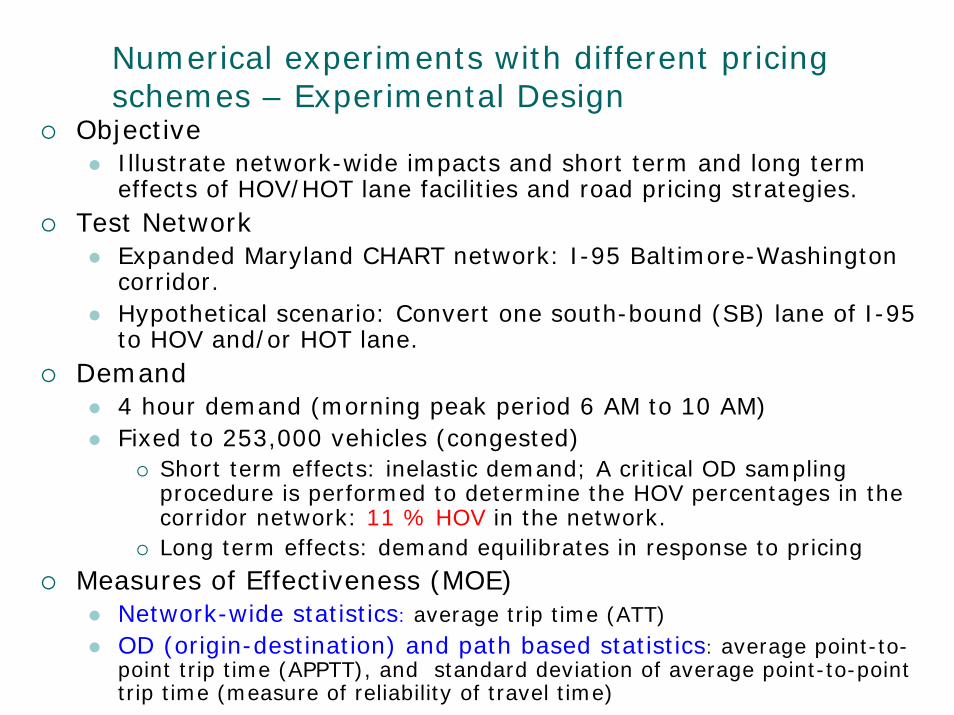
Numerical experiments with different pricing schemes – Experimental Design

ObjectiveIllustrate network-wide impacts and short term and long term effects of HOV/HOT lane facilities and road pricing strategies.

Test NetworkExpanded Maryland CHART network: I-95 Baltimore-Washington corridor.Hypothetical scenario: Convert one south-bound (SB) lane of I-95 to HOV and/or HOT lane.

Demand4 hour demand (morning peak period 6 AM to 10 AM)Fixed to 253,000 vehicles (congested)

Short term effects: inelastic demand; A critical OD sampling procedure is performed to determine the HOV percentages in the corridor network: 11 % HOV in the network.Long term effects: demand equilibrates in response to pricing

Measures of Effectiveness (MOE)Network-wide statistics: average trip time (ATT)OD (origin-destination) and path based statistics: average point-to-point trip time (APPTT), and standard deviation of average point-to-point trip time (measure of reliability of travel time)

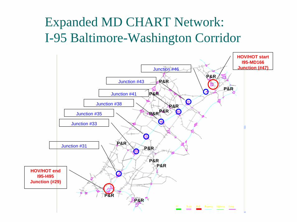
Expanded MD CHART Network: I-95 Baltimore-Washington Corridor

HOV/HOT startI95-MD166

Junction (#47)

HOV/HOT endI95-I495

Junction (#29)

P&RP&R

P&RP&R

P&R

P&R

P&R

P&R

P&RP&RP&R

P&R

P&R

Junction #43

Junction #46

Junction #41

Junction #38

Junction #35

Junction #33

Junction #31

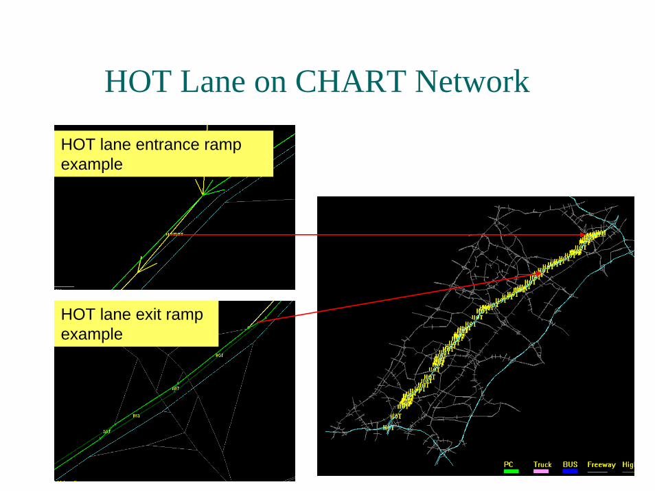
HOT Lane on CHART Network

HOT lane exit ramp example

HOT lane entrance ramp example

Experimental Factors

HOV percentage Fixed to the calculated value 11%

Demand 4 hour demand table (morning peak period 6 AM to 10 AM)Fixed to 253,000 vehicles (congested)LOV 89%HOV 11%

VOTFixed to $ 20 per hour

PricingDistance Based (static)Entry Based (static)Pre-determined time profiles (static-time dependent)

Remarks on short-term effects• Network wide statistics do not provide a sufficient basis to evaluate the

relative performance of HOV or HOT facilities and pricing schemes. Point to point statistics also need to be examined.

• The set of initial HOV/HOT scenarios presented here cannot be directly compared to the base case because the HOV/HOT cases all entail additional links to enable access and egress from the HOV/HOT lanes.

• These scenarios have assumed fixed total demand, with fixed HOV percentage; as such they can be viewed as capturing short term effects of these strategies. However, it would be more meaningful to examine the situation after the demand has had a chance to adjust; the next set of scenarios captures the impact of HOV/HOT and pricing on HOV mode selection in an equilibrium framework.

• The effectiveness of pricing as a traffic management strategy naturally depends on the price set; setting HOT lane prices too low will be counterproductive.

• Adaptive (state-dependent) pricing is recommended for maximum effectiveness as a traffic management tool.

State-Dependent Pricing

Exp: detector locations considered

Uses a logic similar to ramp metering, increments toll value depending on the cut-off density and a gain factor

dc : cut-off densityd : measured density

Price (t)=Price (t-1) + a (d-dc) a : gain factort : time interval

Logic:With the detectors located on specific locations, collect density measure for each time interval and update toll value at each entry ramp.Key issues:Determining • detector locations • gain factor (a)• maximum toll value

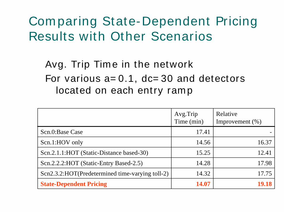
Comparing State-Dependent Pricing Results with Other Scenarios

Avg. Trip Time in the networkFor various a=0.1, dc=30 and detectors

located on each entry ramp

Avg.TripTime (min)

Relative Improvement (%)

Scn.0:Base Case 17.41 -

Scn.1:HOV only 14.56 16.37

Scn.2.1.1:HOT (Static-Distance based-30) 15.25 12.41

Scn.2.2.2:HOT (Static-Entry Based-2.5) 14.28 17.98

Scn2.3.2:HOT(Predetermined time-varying toll-2) 14.32 17.75

State-Dependent Pricing 14.07 19.18

Evaluating Long Term Impacts: Equilibrium Framework

An alternative is a path Prstm(k) which departing from origin r at time t to destination s by mode musing kth route

Modes (HOV and LOV)Routes (with mean trip time and variance)

The disutility for an alternative is related to the generalized cost (GC).

ijtmijtmmijtm GCConstU εα +∗+= 1

where, ijtmGC = generalized cost (GC).

mConst , 1α = utility coefficients

ijtmε = error term

Generalized CostThe generalized cost (GC) is expressed as a function of the path travel time (TT), travel cost (TC), and travel time reliability (which is expressed as travel time standard deviation, TTSD)

β∗++= ijtmijtmijtmijtm TTSDVOTTCTTGC /

Where ijtmTT = path travel time (TT).

ijtmTC = path travel cost (TC).

ijtmTTSD = path travel time reliability or standard deviation (TTSD). VOT = value of time β = reliability ratio, VOTVOR /=β , where VOR is value of reliability.

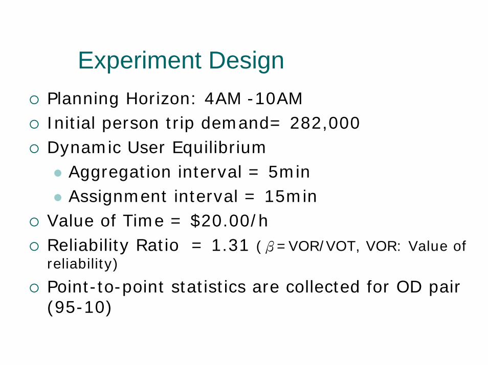
Experiment DesignPlanning Horizon: 4AM -10AMInitial person trip demand= 282,000Dynamic User Equilibrium

Aggregation interval = 5minAssignment interval = 15min

Value of Time = $20.00/hReliability Ratio = 1.31 (β=VOR/VOT, VOR: Value of reliability)

Point-to-point statistics are collected for OD pair (95-10)

Relative Improvement in ATT at Equilibrium w.r.t. Base Case

Scenario Avg. Trip Time Relative Improvement(%)

Scn.0:Base Case 17.41 -

Scn.1:HOV only 14.32 17.75

Scn.2.1.1:HOT (Static-Distance based-30) 14.41 17.23

Scn.2.1.2:HOT (Static-Distance based-40) 14.40 17.29

Scn.2.1.3:HOT (Static-Distance based-50) 14.41 17.23

Scn.2.2.1:HOT (Static-Entry Based-2) 14.30 17.86

Scn.2.2.2:HOT (Static-Entry Based-2.5) 14.46 16.94

Scn.2.2.3:HOT (Static-Entry Based-3.75) 14.34 17.63

Scn.2.3.1:HOT(Predetermined time-varying toll-1) 14.34 17.63

Scn2.3.2:HOT(Predetermined time-varying toll-2) 14.20 18.44

Scn.2.3.3:HOT(Predetermined time-varying toll-3) 14.51 16.66

The ATT among different pricing scenarios do not show a significant difference but they all provide improvement. Scn 2.3.2 performs best in this case.

Relative Improvement in APPTT at Equilibrium w.r.t Base Case

Average Point-to-Point Trip Time (APTT) Relative Improvement (%)

ALL LOV HOV ALL LOV HOV

Do Nothing 26.9 26.9 27.1 - - -

HOV only 28.0 28.2 26.7 -4.1 -4.8 1.5

2.1.1(Distance based-30 cents/mi) 28.90 29.1 27.7 -7.4 -8.2 -2.2

2.1.2(Distance based-40 cents/mi) 28.10 28.2 27.3 -4.5 -4.8 -0.7

2.1.3(Distance based-50 cents/mi) 28.90 29.1 27.7 -7.4 -8.2 -2.2

2.2.1(Entry Based-$2) 26.10 26.2 25.3 3.0 2.6 6.6

2.2.2:HOT (Entry Based-$2.5) 28.90 29 28.3 -7.4 -7.8 -4.4

2.2.3(Entry Based-$3.75) 28.30 28.5 27.1 -5.2 -5.9 0.0

2.3.1(Time-dependent-1) 27.20 27.5 25.7 -1.1 -2.2 5.2

2.3.2:HOT(Time-dependent-2) 26.80 27 25.6 0.4 -0.4 5.5

2.3.3(Time-dependent-3) 28.90 29 28 -7.4 -7.8 -3.3

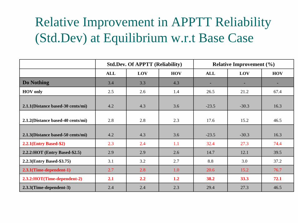
Relative Improvement in APPTT Reliability (Std.Dev) at Equilibrium w.r.t Base Case

Std.Dev. Of APPTT (Reliability) Relative Improvement (%)

ALL LOV HOV ALL LOV HOV

Do Nothing 3.4 3.3 4.3 - - -

HOV only 2.5 2.6 1.4 26.5 21.2 67.4

2.1.1(Distance based-30 cents/mi) 4.2 4.3 3.6 -23.5 -30.3 16.3

2.1.2(Distance based-40 cents/mi) 2.8 2.8 2.3 17.6 15.2 46.5

2.1.3(Distance based-50 cents/mi) 4.2 4.3 3.6 -23.5 -30.3 16.3

2.2.1(Entry Based-$2) 2.3 2.4 1.1 32.4 27.3 74.4

2.2.2:HOT (Entry Based-$2.5) 2.9 2.9 2.6 14.7 12.1 39.5

2.2.3(Entry Based-$3.75) 3.1 3.2 2.7 8.8 3.0 37.2

2.3.1(Time-dependent-1) 2.7 2.8 1.0 20.6 15.2 76.7

2.3.2:HOT(Time-dependent-2) 2.1 2.2 1.2 38.2 33.3 72.1

2.3.3(Time-dependent-3) 2.4 2.4 2.3 29.4 27.3 46.5

Change of HOV Mode Share at Equilibrium

HOV Mode Share at Dynamic User Equilibrium

10.8

11.0

11.2

11.4

11.6

11.8

12.0

12.2

12.4

1 2 3 4 5

Iteration

HO

V Sp

lit (%

)

WithoutHOV/HOTHOV only

2.1.1

2.1.2

2.1.3

2.2.1

2.2.2

2.2.3

2.3.1

2.3.2

2.3.3

Remarks on long-term effects

The point-to-point statistics suggest that average point-to-point trip time with different pricing scenarios may not necessarily improve for all OD pairsHowever, the std. dev. of average point-to-point trip time (reliability) improves significantly in most cases, especially for HOVsAgain, entry-based and time-dependent pricing schemes had close performance and gave better results than the other pricing strategies testedHOV mode share is highest in HOV only case which is expected, because lane is devoted only to HOVsPricing provides a significant increase in HOV mode share in short term All pricing scenarios improved HOV mode share in long term with respect to base case (11%)

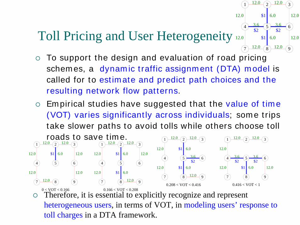
Toll Pricing and User Heterogeneity To support the design and evaluation of road pricing schemes, a dynamic traffic assignment (DTA) model is called for to estimate and predict path choices and the resulting network flow patterns.

Empirical studies have suggested that the value of time (VOT) varies significantly across individuals; some trips take slower paths to avoid tolls while others choose toll roads to save time.

1 2 3

4 5 6

7 8 9

12.0 12.0

12.0 12.0

12.0

12.0

12.0

12.0

3.6 3.6$2$2

6.0

6.0

$1

$1

1 2 3

4 5 6

7 8 9

12.0 12.0

12.0

12.0

12.0

3.6 3.6$2$2

6.0$1

0.416 < VOT < 1

1 2 3

4 5 6

7 8 9

12.0 12.0

12.0

12.0

12.0

3.6$2

6.0

6.0

$1

$1

0.208 < VOT < 0.416

1 2 3

4 5 6

7 8 9

12.0 12.0

12.0

12.012.0

12.0

6.0

6.0

$1

$1

0.166 < VOT < 0.208

1 2 3

4 5 6

7 8 9

12.0 12.0

12.0

12.0

12.0

12.0

12.0

6.0$1

0 < VOT < 0.166Therefore, it is essential to explicitly recognize and representheterogeneous users, in terms of VOT, in modeling users’ response to toll charges in a DTA framework.

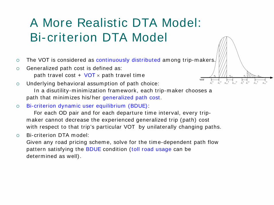
A More Realistic DTA Model: Bi-criterion DTA Model

The VOT is considered as continuously distributed among trip-makers.

Generalized path cost is defined as: path travel cost + VOT × path travel time

Underlying behavioral assumption of path choice:In a disutility-minimization framework, each trip-maker chooses a

path that minimizes his/her generalized path cost.

Bi-criterion dynamic user equilibrium (BDUE):For each OD pair and for each departure time interval, every trip-

maker cannot decrease the experienced generalized trip (path) cost with respect to that trip’s particular VOT by unilaterally changing paths.

Bi-criterion DTA model:Given any road pricing scheme, solve for the time-dependent path flow pattern satisfying the BDUE condition (toll road usage can be determined as well).

kα

lbkα

ubkα

1+kα

lbk 1+α ub

k 1+αVOT

lα

ublα

1+lα

lbl 1+αlb

lαub

l 1+α

Experimental Results –Time-dependent Toll Road Usage

0.7

0.75

0.8

0.85

0.9

0.95

1

1.05

10 15 20 25 30 35 40 45 50

Time (minutes)

Toll

Roa

d U

sage

(x10

0%

Constant(20)Discrete VOTN(20,10)

0.3

0.4

0.5

0.6

0.7

0.8

0.9

10 15 20 25 30 35 40 45 50

Time (minutes)

Toll

Roa

d U

sage

(x10

0%

Constant(20)Discrete VOTN(20,10)

Constant and discrete VOT models overestimate time-dependent toll road usage when the toll charge is low.

Constant and discrete VOT models underestimate time-dependent toll road usage when the toll charge is high.

Concluding RemarksPricing increasingly part of integrated management of the transportation infrastructureNeed for dynamic network analysis methods to evaluate alternative pricing schemes in combination with ITS measuresEffectiveness of pricing during congested peak periods depends on judicious use of advanced methods coupled with sensor technologiesTime-varying prices strongly preferred to static prices; real-time anticipatory pricing conceptually bestThe next frontier: pricing as part of coordinated policies for aggressive demand managementIssues: user and political acceptability (waning opposition); different prices for different user classes (e.g. trucks ); equity