Embed Size (px)
Citation preview
EVALUATION OF RESILIENT MODULUS ESTIMATION METHODS FOR
ASPHALT MIXTURES BASED ON LABORATORY MEASUREMENTS
A THESIS SUBMITTED TO
THE GRADUATE SCHOOL OF NATURAL AND APPLIED SCIENCES
OF
MIDDLE EAST TECHNICAL UNIVERSITY
BY
CANSER DEMİRCİ
IN PARTIAL FULFILLMENT OF THE REQUIREMENTS
FOR
THE DEGREE OF MASTER OF SCIENCE
IN
CIVIL ENGINEERING
APRIL 2010

Approval of the thesis:
EVALUATION OF RESILIENT MODULUS ESTIMATION METHODS FOR
ASPHALT MIXTURES BASED ON LABORATORY MEASUREMENTS
submitted by CANSER DEMİRCİ in partial fulfillment of the requirements for the
degree of Master of Science in Civil Engineering Department, Middle East
Technical University by,
Prof. Dr. Canan Özgen
Dean, Graduate School of Natural and Applied Sciences __________________
Prof. Dr. Güney Özcebe
Head of Department, Civil Engineering __________________
Assoc. Prof. Dr. Murat Güler
Supervisor, Civil Engineering Dept., METU __________________
Examining Committee Members:
Prof. Dr. Özdemir AKYILMAZ
Civil Engineering Dept., METU __________________
Assoc. Prof. Dr. Murat Güler
Civil Engineering Dept., METU __________________
Assoc. Prof. Dr. Ġsmail Özgür Yaman
Civil Engineering Dept., METU __________________
Dr. Soner Osman Acar
Civil Engineering Dept., METU __________________
Assist. Prof. Dr. Hikmet Bayırtepe
Civil Engineering Dept., Gazi University __________________
Date: __________________

iii
I hereby declare that all information in this document has been obtained and
presented in accordance with academic rules and ethical conduct. I also declare
that, as required by these rules and conduct, I have fully cited and referenced
all material and results that are not original to this work.
Name, Last name: Canser DEMĠRCĠ
Signature:
iv
ABSTRACT
EVALUATION OF RESILIENT MODULUS ESTIMATION METHODS FOR
ASPHALT MIXTURES BASED ON LABORATORY MEASUREMENTS
Demirci, Canser
M.S., Department of Civil Engineering
Supervisor: Assoc. Prof. Dr. Murat Güler
April 2010, 69 Pages
Resilient modulus is a property for bound and unbound pavement materials
characterizing the elastic behavior of materials under dynamic repeated loading.
Resilient modulus is an important design parameter for pavement structures because
it represents the structural strength of pavement layers through which the thickness
design is based on. In Turkey, the layer thickness design is performed using resilient
modulus determined empirically from various published sources. Determining a
layer modulus using empirical methods causes inaccurate design solutions, which
directly affects the structural performance and the overall cost of pavement
construction. In this study, the resilient moduli of bituminous mixtures are measured
in the laboratory by the indirect tensile test procedure for eight asphalt concrete
samples according to NCHRP and ASTM procedures. The measured moduli of
samples based on the two procedures are compared with the predicted values
calculated from various empirical methods using aggregate and binder properties. An
evaluation of each estimation method is presented on the basis of its accuracy level.
The results show that the Witczak predictive equation produces the closest estimation
to the modulus of samples for both laboratory measurement methods.
Key words: Resilient Modulus, Indirect Tension Test, Mix Stiffness
v
ÖZ
ESNEKLĠK MODÜLÜ TAHMĠN YÖNTEMLERĠNĠN LABORATUVAR DENEY
SONUÇLARINA DAYANARAK DEĞERLENDĠRĠLMESĠ
Demirci, Canser
Yüksek lisans, ĠnĢaat Mühendisliği Bölümü
Tez Yöneticisi: Doç. Dr. Murat Güler
Mayıs 2010, 69 Sayfa
Esneklik modülü bağlayıcılı be bağlayıcısız üstyapı malzemeleri için dinamik tekrarlı
yükler altında elastik davranıĢını gösteren bir özelliktir. Esneklik modülü üstyapı
malzemelerinin kalınlık dizaynı yapılırken kullanılan yapısal dayanımını
göstermesinden dolayı üstyapı için önemli bir parametredir. Türkiye’de tabaka
kalınılk dizaynı yapılırken esneklik modülü yayınlanmıĢ çeĢitli kaynaklardan ampirik
olarak alınır. Ampirik olarak elde edilen bir tabaka modülünün kullanılması
üstyapının yapısal dayanımını ve toplam maliyetini direk olarak etkileyen hatalı
dizayn sonuçlarına neden olabilir. Bu çalıĢmada bitümlü karıĢımların esneklik
modülleri, sekiz farklı karıĢım için laboratuvarda indirek çekme deneyi ile ölçüldü.
Numunelerin ölçülen modülleri agrega ve bitüm özelliklerini kullanan çeĢitli ampirik
yöntemlerle tahmin edilen değerlerle karĢılaĢtırılılmıĢtır. Her bir tahmin yönteminin
değerlendirilmesi, doğruluk derecesine bağlı olarak sunulmuĢtur. Sonuçlar, Witczak
tahmin denklemlerinin deney ölçümlerine en yakın sonuçları verdiğini
göstermektedir.
Anahtar kelimeler: Esneklik Modülü, Ġndirekt Çekme Deneyi, KarıĢım Rijitliği

vi
To my family.

vii
ACKNOWLEDGMENTS
I greatly acknowledge the guidance and encouragement of my supervisor, Assoc.
Prof. Dr. Murat Güler, for his kindness, sincere advices, understanding, and patience
on listening to my questions throughout the study.
I would also like to thank to Turkish General Directorate of Highways (TGDH)
pavement division director, Ahmet Gürkan Güngör and engineer Ahmet Sağlık for their
continual help during my graduate study.
I deeply appreciate my fellow workers of Turkish General Directorate of Highways
(TGDH) pavement division laboratory.
I am also thankful to my parents for their supports and good wishes through my
whole life and this study.
Finally, I would also like to thank to my wife Özlem, for her encouragements, support
and patience during my study, and my daughter Özüm Zeynep for her endless smiles.
viii
TABLE OF CONTENTS
ABSTRACT ................................................................................................................ iv
ÖZ ................................................................................................................................ v
ACKNOWLEDGEMENTS ....................................................................................... vii
TABLE OF CONTENTS .......................................................................................... viii
LIST OF TABLES ....................................................................................................... x
LIST OF FIGURES .................................................................................................... xi
LIST OF SYMBOLS ................................................................................................ xiii
CHAPTER
1.INTRODUCTION .................................................................................................... 1
1.1 Background ....................................................................................................... 1
1.2 Objective of the Study ....................................................................................... 2
1.3 Scope ................................................................................................................. 2
2. LITERATURE REVIEW.. .......................................................................................3
2.1 Introduction ....................................................................................................... 3
2.2 Resilient modulus ............................................................................................. 3
2.3 Determination of Resilient Modulus ................................................................ 4
2.4 Indirect Tension Test for Determining Resilient Modulus .............................. 5
2.5 Stiffness of Bitumen ......................................................................................... 6
2.6 Estimation of Resilient Modulus of Asphalt Mixtures ..................................... 9
3. MATERIALS AND METHOD ............................................................................ 14
3.1 Introduction ..................................................................................................... 14
3.2 Materials Used for Experiments ..................................................................... 14
3.2.1 Aggregate Caharacteristics ........................................................................ 14
3.2.2 Bitumen Characteristics ............................................................................. 15
3.2.3 Specimen Preparation ................................................................................ 16
3.3 Indirect Tension Test for Determining Resilient Modulus of Bituminous
Mixtures ................................................................................................................. 23
ix
3.3.1 Test Equipment .......................................................................................... 23
3.3.2 Test Procedure ........................................................................................... 24
3.3.3 Test Results ................................................................................................ 30
4.DETERMINATION OF RESILIENT MODULUS BY NOMOGRAPHS AND
EQUATIONS ............................................................................................................ 41
4.1 Van Der Poel and Shell Nomographs ............................................................. 41
4.1.1 Van Der Poel Nomograph ......................................................................... 41
4.1.2 Shell Nomograph ...................................................................................... 42
4.2 Estimation of the Resilient Modulus of the Mixes by Equations .................... 45
4.2.1 Estimation of the Stiffness of the Bitumen by Equation ............................ 45
4.2.2 Estimation of the Resilient Modulus of the Mixtures by Equations .......... 45
4.2.3 Discussion of Results ................................................................................. 56
5. CONCLUSIONS ................................................................................................... 63
REFERENCES ........................................................................................................... 65
APPENDIX
A. Indirect tension test set up parameters and test results. ................................ 68
x
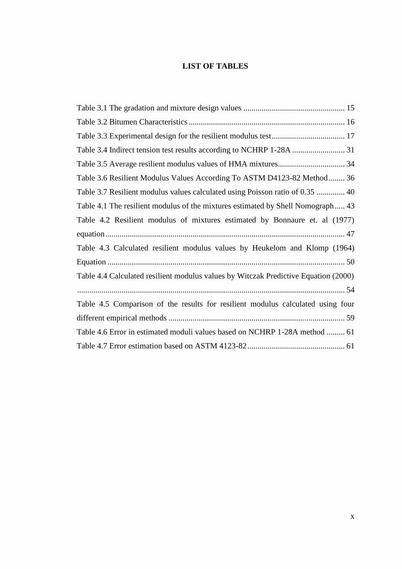
LIST OF TABLES
Table 3.1 The gradation and mixture design values .................................................. 15
Table 3.2 Bitumen Characteristics ............................................................................. 16
Table 3.3 Experimental design for the resilient modulus test .................................... 17
Table 3.4 Indirect tension test results according to NCHRP 1-28A .......................... 31
Table 3.5 Average resilient modulus values of HMA mixtures................................. 34
Table 3.6 Resilient Modulus Values According To ASTM D4123-82 Method ........ 36
Table 3.7 Resilient modulus values calculated using Poisson ratio of 0.35 .............. 40
Table 4.1 The resilient modulus of the mixtures estimated by Shell Nomograph ..... 43
Table 4.2 Resilient modulus of mixtures estimated by Bonnaure et. al (1977)
equation ...................................................................................................................... 47
Table 4.3 Calculated resilient modulus values by Heukelom and Klomp (1964)
Equation ..................................................................................................................... 50
Table 4.4 Calculated resilient modulus values by Witczak Predictive Equation (2000)
.................................................................................................................................... 54
Table 4.5 Comparison of the results for resilient modulus calculated using four
different empirical methods ....................................................................................... 59
Table 4.6 Error in estimated moduli values based on NCHRP 1-28A method ......... 61
Table 4.7 Error estimation based on ASTM 4123-82 ................................................ 61
xi
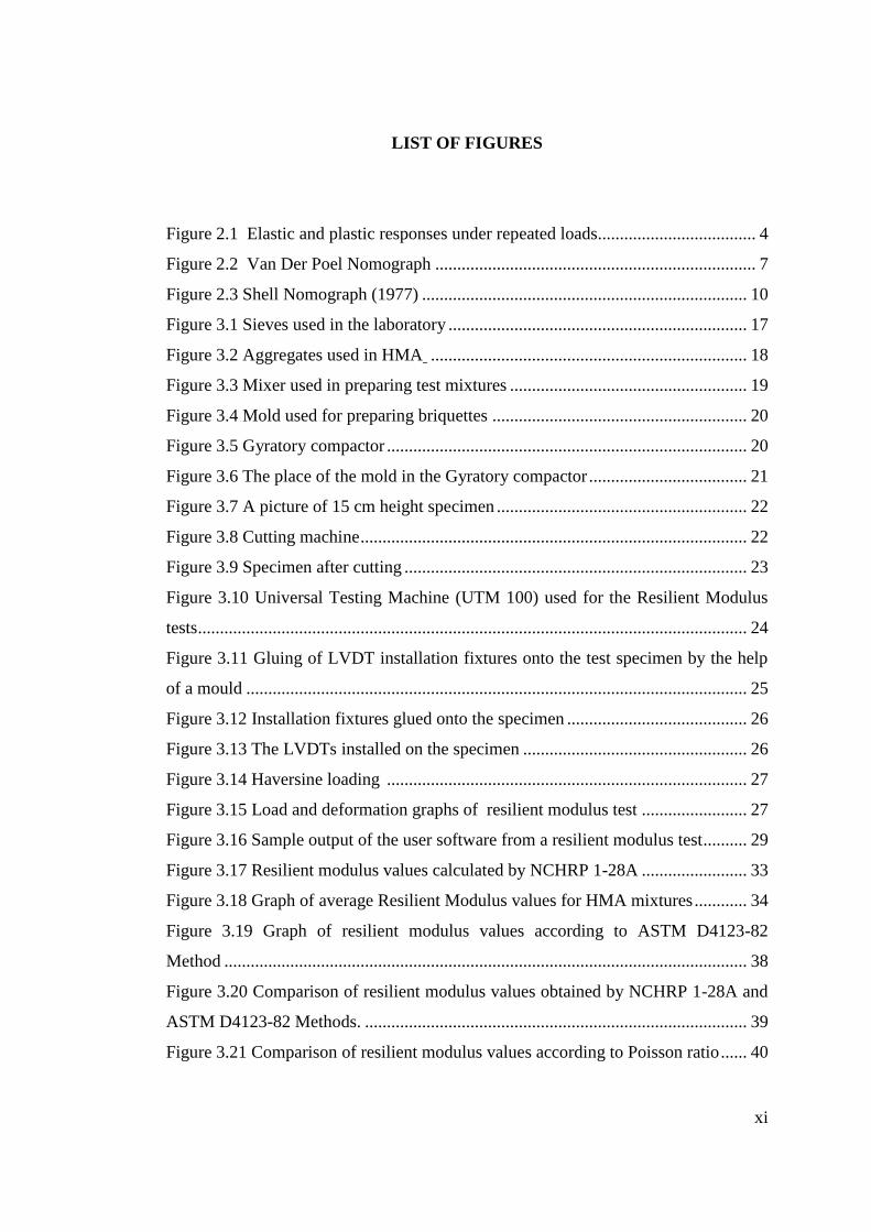
LIST OF FIGURES
Figure 2.1 Elastic and plastic responses under repeated loads.................................... 4
Figure 2.2 Van Der Poel Nomograph ......................................................................... 7
Figure 2.3 Shell Nomograph (1977) .......................................................................... 10
Figure 3.1 Sieves used in the laboratory .................................................................... 17
Figure 3.2 Aggregates used in HMA ........................................................................ 18
Figure 3.3 Mixer used in preparing test mixtures ...................................................... 19
Figure 3.4 Mold used for preparing briquettes .......................................................... 20
Figure 3.5 Gyratory compactor .................................................................................. 20
Figure 3.6 The place of the mold in the Gyratory compactor .................................... 21
Figure 3.7 A picture of 15 cm height specimen ......................................................... 22
Figure 3.8 Cutting machine ........................................................................................ 22
Figure 3.9 Specimen after cutting .............................................................................. 23
Figure 3.10 Universal Testing Machine (UTM 100) used for the Resilient Modulus
tests ............................................................................................................................. 24
Figure 3.11 Gluing of LVDT installation fixtures onto the test specimen by the help
of a mould .................................................................................................................. 25
Figure 3.12 Installation fixtures glued onto the specimen ......................................... 26
Figure 3.13 The LVDTs installed on the specimen ................................................... 26
Figure 3.14 Haversine loading .................................................................................. 27
Figure 3.15 Load and deformation graphs of resilient modulus test ........................ 27
Figure 3.16 Sample output of the user software from a resilient modulus test .......... 29
Figure 3.17 Resilient modulus values calculated by NCHRP 1-28A ........................ 33
Figure 3.18 Graph of average Resilient Modulus values for HMA mixtures ............ 34
Figure 3.19 Graph of resilient modulus values according to ASTM D4123-82
Method ....................................................................................................................... 38
Figure 3.20 Comparison of resilient modulus values obtained by NCHRP 1-28A and
ASTM D4123-82 Methods. ....................................................................................... 39
Figure 3.21 Comparison of resilient modulus values according to Poisson ratio ...... 40

xii
Figure 4.1 Graph of the resilient modulus values calculated by Shell Nomograph
(1977). ........................................................................................................................ 44
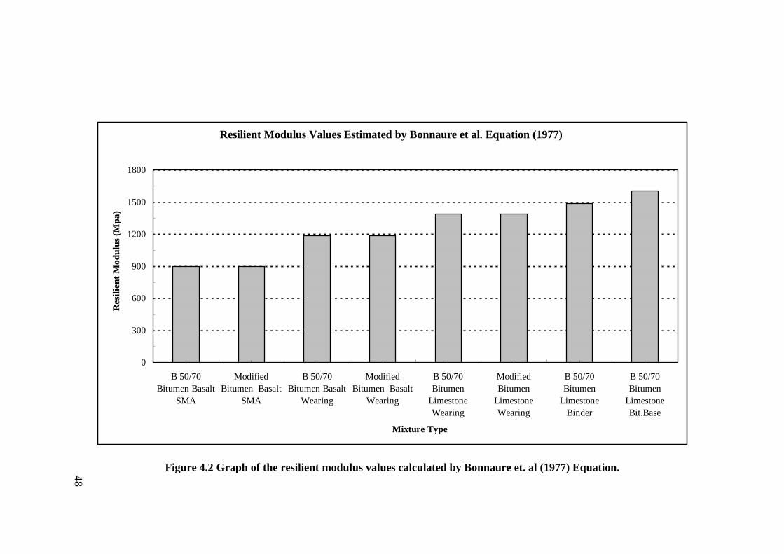
Figure 4.2 Graph of the resilient modulus values calculated by Bonnaure et. al (1977)
Equation. .................................................................................................................... 48
Figure 4.3 Stiffness values calculated by Heukelom-Klomp (1964) equation .......... 51
Figure 4.4 Resilient Modulus values calculated by Witczak predictive equation
(2000) ......................................................................................................................... 55
Figure 4.5 Comparison of Resilient Modulus values based on ASTM and NCHRP
methods ...................................................................................................................... 57
Figure 4.6 Comparison of Resilient Modulus values obtained by Empirical Methods
with Experimental Results ......................................................................................... 60
Figure 4.7 Percent error values for empirical methods used ...................................... 62
xiii
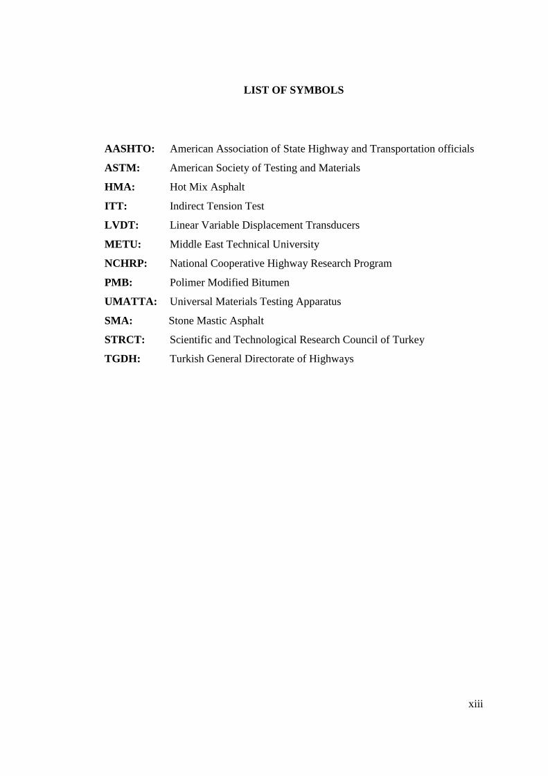
LIST OF SYMBOLS
AASHTO: American Association of State Highway and Transportation officials
ASTM: American Society of Testing and Materials
HMA: Hot Mix Asphalt
ITT: Indirect Tension Test
LVDT: Linear Variable Displacement Transducers
METU: Middle East Technical University
NCHRP: National Cooperative Highway Research Program
PMB: Polimer Modified Bitumen
UMATTA: Universal Materials Testing Apparatus
SMA: Stone Mastic Asphalt
STRCT: Scientific and Technological Research Council of Turkey
TGDH: Turkish General Directorate of Highways
1
CHAPTER 1
INTRODUCTION
1.1 Background
In order to design a long lasting pavement, it is very important to estimate the actual
field conditions in design phase of asphalt concrete pavements. For example, better
structural performance depends on a good projection of future traffic and accurate
representation of field conditions, i.e., temperature. Traffic loads are represented by
cyclic loads in the performance testing of asphalt mixtures, and the resilient modulus
is used to describe the stress-strain behavior of asphalt concrete under cyclic traffic
loading. It is the most important material parameter in the design process of asphalt
concrete pavements characterizing the entire structural performance of pavement
structure. Hence, the accurate estimation of resilient modulus directly affects the
layer thickness, service life and the overall cost of the pavement construction.
In Turkey, according to the Highway Flexible Pavement Design Guide published by
the Turkish General Directorate of Highways, which is based on AASHTO 1993
design procedures, the resilient modulus of structural layers are used to estimate the
layer coefficients hence layer thicknesses. These resilient modulus values are
estimated from various nomographs or empirical relations, which are questionable in
terms of reliability and accuracy. It is obvious that a deviation between the estimated
and the actual modulus may easily cause inaccurate design solutions. Hence, the
Turkish General Directorate of Highways (TGDH) started a research project that was
funded by the Scientific Technological Research Council of Turkey’s (STRCT)
under the project 105G021 “Adaptation of Resilient Modulus to Mechanistic-
Empirical Design Specifications of Flexible Pavements”. A major portion of this
project was assigned for testing resilient modulus of bound, i.e., asphalt concrete,
materials. A comparison of various empirical methods is conducted based on this
research outcomes, and the method leading to the closest approximation to the
measured modulus values are presented accordingly.

2
1.2 Objective of the Study
The objective of this study is (i) to determine the resilient modulus of Hot Mix
Asphalt (HMA) mixtures which are prepared by different aggregate and bitumen
types suggested in the Turkish General Directorate of Highways design guidelines;
(ii) to estimate the resilient modulus of the HMA mixtures by empirical methods; iii)
to compare the results obtained by laboratory measurements and estimation methods
and; (iv) to choose the empirical method that best approximates the laboratory
measurements by comparing the results.
1.3 Scope
This study consists of three main parts: First part is the determination of resilient
modulus of HMA mixtures used in the design of asphalt concrete pavements in
Turkey. For this purpose, eight different types of mixtures which are used in Turkey
were prepared and subjected to the resilient modulus testing in TGDH Technical
Research Department Laboratories. The tests were conducted according to the
NCHRP 1-28A guidelines using an UTM-100 machine under 25 0C temperature.
The resilient modulus values were calculated according to both NCHRP 1-28A and
ASTM D4123-82 procedures.
The second part includes the estimation of resilient modulus of bituminous mixtures
by nomographs and empirical equations. The nomographs and the equations are used
to calculate the resilient modulus values based on various volumetric and rheological
properties of mix constituents, i.e., aggregate and asphalt binder.
Finally, in the third part, a discussion is given on the reliability and the accuracy of
both empirical and graphical methods in estimating the measured resilient modulus
values.
3
CHAPTER 2
LITERATURE REVIEW
2.1 Introduction
In this chapter, various literatures taken from different sources about resilient
modulus and materials characteristics are presented. In the first part, the definition
and the determination of resilient modulus are elaborated. Then, information about
the bitumen and aggregate characteristics ıs given. Finally, the determination of
HMA mix stiffness by using bitumen stiffness is explained.
2.2 Resilient Modulus
The AASHTO Pavement Design Guide (1993), in addition to other revisions,
incorporated the resilient modulus (MR) concept to characterize pavement materials
subjected to moving traffic loads. MR values may be estimated directly from
laboratory testing, indirectly through correlation with other laboratory/field tests, or
back calculated from deflection measurements. The testing procedure for the
determination of MR consists of the application of a repeated deviator stress (ζd),
under a constant cell pressure and then measuring the resilient axial strain. Under
repeated load tests, it is observed that as the number of load cycles increases, the
secant modulus increases. After a number of load cycles, the modulus becomes
nearly constant, and the response can be presumed to be elastic. This steady value of
modulus is defined as the resilient modulus (Rahim A.M., 2005).
The actual resilient response of a material under repeated loading can be determined
after a certain number of load applications since there would be considerable
permanent deformation within the early stages. As the number of load applications
increases, the plastic strains due to load repetition decreases (Huang, 1993). Thus,
the resilient modulus for a certain sequence is determined using the last 5
measurements out of 100 readings. The resilient modulus is defined as the ratio of
4
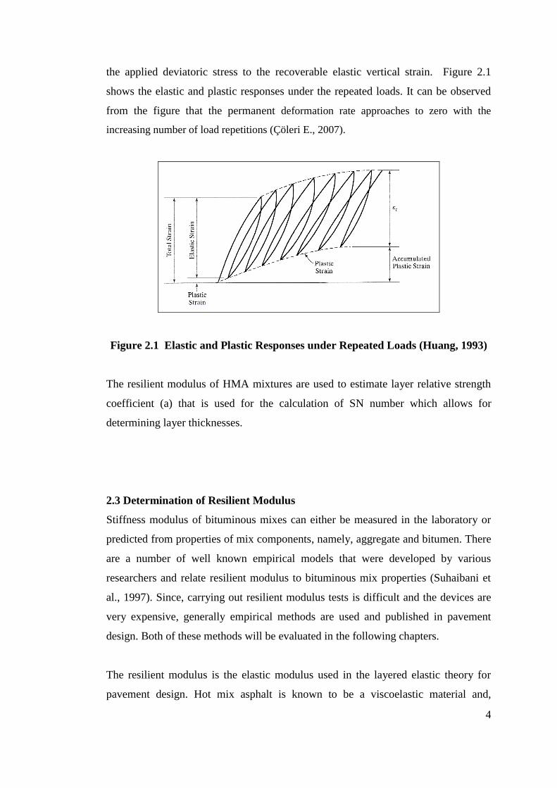
the applied deviatoric stress to the recoverable elastic vertical strain. Figure 2.1
shows the elastic and plastic responses under the repeated loads. It can be observed
from the figure that the permanent deformation rate approaches to zero with the
increasing number of load repetitions (Çöleri E., 2007).
Figure 2.1 Elastic and Plastic Responses under Repeated Loads (Huang, 1993)
The resilient modulus of HMA mixtures are used to estimate layer relative strength
coefficient (a) that is used for the calculation of SN number which allows for
determining layer thicknesses.
2.3 Determination of Resilient Modulus
Stiffness modulus of bituminous mixes can either be measured in the laboratory or
predicted from properties of mix components, namely, aggregate and bitumen. There
are a number of well known empirical models that were developed by various
researchers and relate resilient modulus to bituminous mix properties (Suhaibani et
al., 1997). Since, carrying out resilient modulus tests is difficult and the devices are
very expensive, generally empirical methods are used and published in pavement
design. Both of these methods will be evaluated in the following chapters.
The resilient modulus is the elastic modulus used in the layered elastic theory for
pavement design. Hot mix asphalt is known to be a viscoelastic material and,
5
therefore, experiences permanent deformation after each application of load cycle.
However, if the load is small compared to the strength of the material and after a
relatively large number of repetitions (100 to 200 load repetitions), the deformation
after the load application is almost completely recovered. The deformation is
proportional to the applied load and since it is nearly completely recovered it can be
considered as elastic.
For unbound materials, the resilient modulus is based on the recoverable strain under
repeated loading and is determined as follows:
r
rM
d (2.1)
where ζd is the deviator stress and εr is the recoverable (resilient strain). Because the
applied load is usually small compared to the strength of the specimen, the same
specimen may be used for the same test under different loading and temperatures
(Katicha W.S., 2003)
The resilient modulus can be performed on laboratory prepared specimens or field
cores. For consistency in design, results obtained from laboratory prepared
specimens should match with results obtained from field cores (Katicha W.S., 2003)
2.4 Resilient Modulus Test
Resilient modulus testing, developed by Seed et al. (1962), aims to determine an
index that describes the nonlinear stress-strain behavior of soils under cyclic loading.
Resilient modulus is simply the ratio of the dynamic deviatoric stress to the
recovered strain under a standard haversine pulse loading. Mechanistic design
procedures for pavements and overlays require resilient modulus of unbound
pavement layers to determine layer thickness and the overall system response to
traffic loads. In AASHTO specification T-274 (1982) based on the mechanistic
methods, resilient modulus is considered as an important design input parameter.
After this specification, AASHTO TP46, T292, T294 and T307 specifications were

6
also published as improvements were made over the years in the test procedures
(Çöleri, E., 2007)
Different test methods and equipment have been developed and employed to measure
these different moduli. Some of the tests employed are triaxial tests (constant and
repeated cyclic loads), cyclic flexural test, indirect tensile tests (constant and
repeated cyclic load), and creep test. Baladi and Harichandran indicated that resilient
modulus measurement by indirect tensile test is the most promising in terms of
repeatability. Resilient modulus measured in the indirect tensile mode (ASTM D
4123-82) has been selected by most engineers as a method to measure the resilient
modulus of asphalt mixes (Brown et al., 1989)
NCHRP (National Cooperative Highway Research Program) Project 1-28A
“Recommended Standard Test Method For Determining the Resilient Modulus of
Bituminous Mixtures by Indirect Tension” is the latest method in AASHTO standard
format.
2.5 Stiffness of the Bitumen
Stiffness of the bitumen used in the mix is an important parameter that affects the
stiffness of the mix directly.
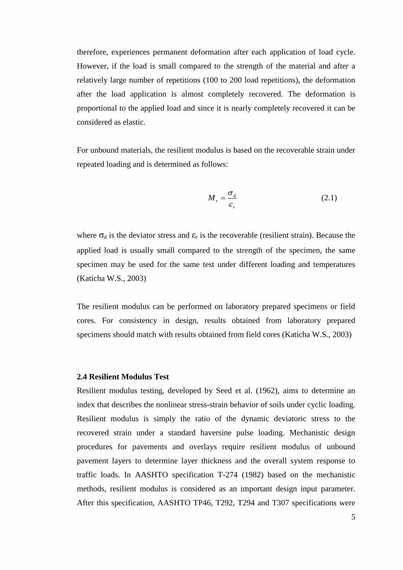
Van Der Poel developed one of the first stiffness prediction models for asphalt
concrete (Figure 2.2). It is one of the most commonly used models to predict the
stiffness modulus of bitumen as a function of time of loading, the penetration index,
and the temperature at which the penetration of the bitumen is 800 (Suhaibani et al.,
1997).
7
Figure 2.2 Van Der Poel Nomograph (After Huang, 2004)
8
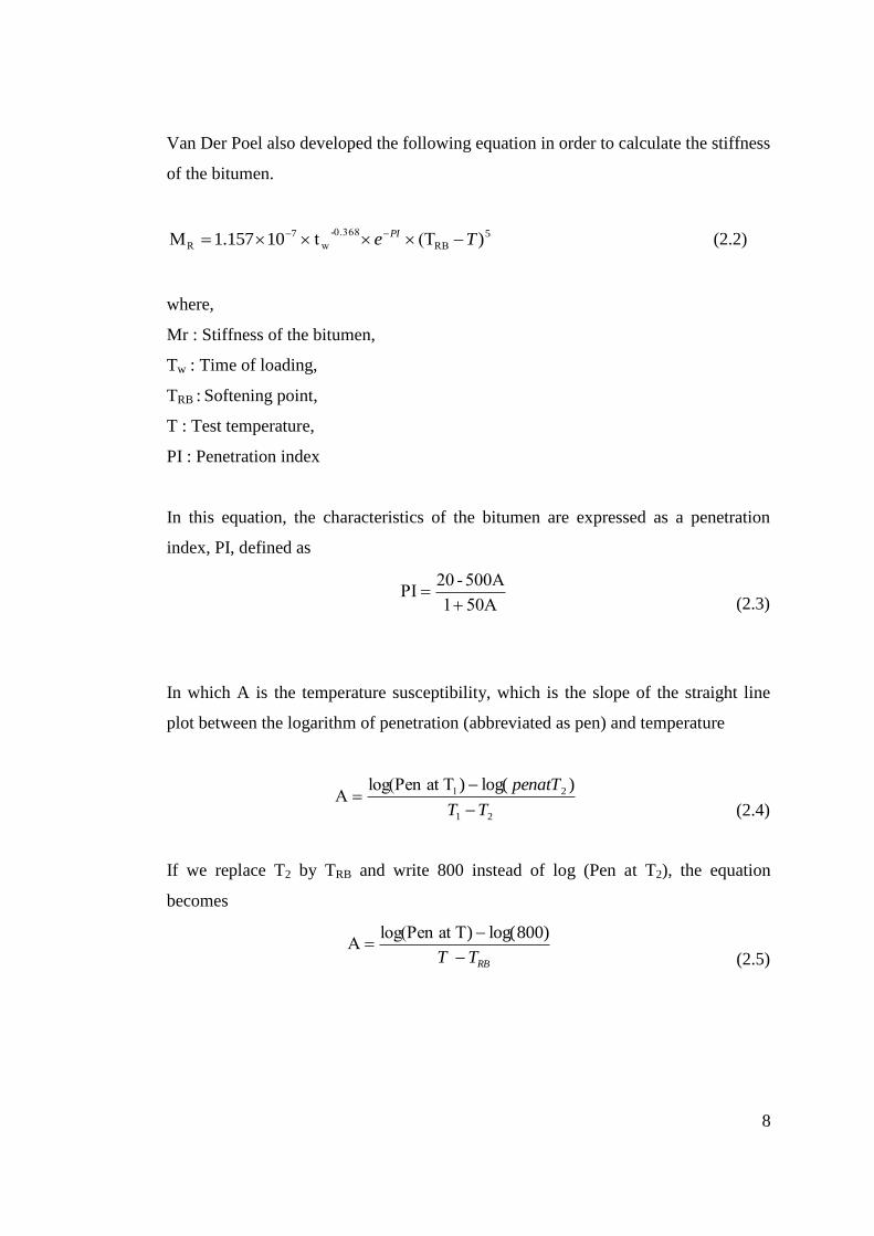
Van Der Poel also developed the following equation in order to calculate the stiffness
of the bitumen.
57 )10157.1 Te PI
RB
-0.368
wR (Tt M (2.2)
where,
Mr : Stiffness of the bitumen,
Tw : Time of loading,
TRB : Softening point,
T : Test temperature,
PI : Penetration index
In this equation, the characteristics of the bitumen are expressed as a penetration
index, PI, defined as
50A1
500A-20PI
(2.3)
In which A is the temperature susceptibility, which is the slope of the straight line
plot between the logarithm of penetration (abbreviated as pen) and temperature
21
2 )log()
TT
penatT
1Tat log(Pen
A (2.4)
If we replace T2 by TRB and write 800 instead of log (Pen at T2), the equation
becomes
RBTT
)800log()Tat log(PenA
(2.5)

9
2.6 Estimation of Resilient Modulus of Asphalt Mixture
The resilient modulus of bituminous mixtures can also be determined by nomographs
and some empirical equations that use stiffness of the bitumen, volume of the
bitumen and the aggregate in the mixture.
Shell Nomograph (1977)
Figure 2.3 shows the nomograph for determining the stiffness modulus of the
bituminous mixtures (Bonnaure et al.,1977) Three factors considered are the stiffness
modulus of bitumen, the percent volume of bitumen and the percent volume of
aggregate.
The percent volume of aggregate Vg is
g
mb
m G
GP
GW
)1(100100
/
gb
g
)W/GP-(1V
(2.6)
The percent volume of bitumen Vb is
b
mb
m G
GP
GW
100100
/ bb
b
W/GPV
(2.7)
The percent volume of air void Va is
Va = 100- Vg - Vb (2.8)
where,
Gm : The bulk specific gravity of mixture
W : Total weight of mixture

10
Figure 2.3 Shell Nomograph (After Huang, 2004)
Bonnaure et al. Equation (1977)
Bonnaure et al. (1977) also developed the following equation for predicting the
resilient modulus of mix Sm, based on Vg, Vb, and Sb (Huang, 1993)
bg VV
gV-1,342(100
82,101 (2.9)
11
2
2 0002135,00568,00,8 gg VV (2.10)
133,1
)1log(6,03
bV
2
b1,37V (2.11)
)(7582,0 214 (2.12)
For 5 x 10⁶ N/m
2<Sb<10
9 N/m
2
2
34 8log2
)8(log2
log
bbm SSS 31 (2.13)
For 109 N/m
2<Sb<3 x 10
9 N/m
2
)9log()(0959,2log 42142 bm SS (2.14)
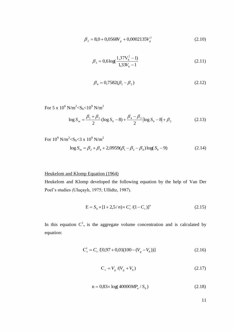
Heukelom and Klomp Equation (1964)
Heukelom and Klomp developed the following equation by the help of Van Der
Poel’s studies (Uluçaylı, 1975; Ullidtz, 1987).
n
v
ı
vb CCnS )]1/()/5,21[ E (2.15)
In this equation C1
v is the aggregate volume concentration and is calculated by
equation:
))](100(01,097,0/[ bgv VVC 1
vC (2.16)
)/( bgg VVV vC (2.17)
)/40000log(83,0 ba SMPn (2.18)

12
Asphalt Institute (1979) Equations
In developing the DAMA computer program for the Asphalt Institute, Hwang and
Witzack (1979) applied the following regression formulas to determine the dynamic
modulus of HMA, |E*| :
110100000* E (2.19)
1.1
2231 00189.0000005.0 f (2.20)
55.0
42
T (2.21)
02774.0
1703.0
2003
931757.0070377.0
03476.0028829.0553833.0
f
VfP a
(2.22)
bV483.04 (2.23)
flog492825.03.15 (2.24)
In these equations, β1 to β5 are temporary constants, f is the load frequency in Hz, T
is the temperature in 0F, P200 is the percentage by weight of aggregate passing
through a No.200 sieve, Vv is the volume of air void in %, λ is the asphalt viscosity
at 70 0F in 10
6 poise, and Vb is the volume of bitumen in %. If sufficient viscosity
data are not available to estimate λ at 70 0F, one may use the equation
1939.2
7702.29508
F
P (2.25)
In which P770
F is the penetration at 77 0F (25
0C). (Huang, 1993)
Witczak Predictive Equation (2000)
After this first study, Witczak and Fonseca (1995) propose an empirical model to
predict the complex modulus of an asphalt mixture. The proposed model for complex
modulus master curve was generated based on a large amount of data consisting of
1429 points from 149 separate asphalt mixtures. Improvements were made to earlier
models, taking into account hardening effects from short- and long-term aging, as
well as extreme temperature conditions. Based on the gradation of aggregates in the
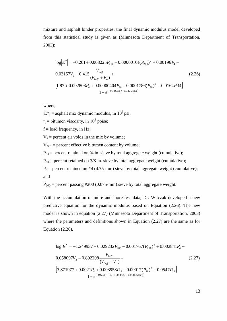
13
mixture and asphalt binder properties, the final dynamic modulus model developed
from this statistical study is given as (Minnesota Department of Transportation,
2003):
log7425.0log716.0
2
38384
4
2
200200
*
1
340164.0)(0001786.000000404.0002808.087.1
)(415.003157.0
00196.0)(00000101.0008225.0261.0log
f
abeff
beff
a
e
PPPP
VV
VV
PPPE
(2.26)
where,
|E*| = asphalt mix dynamic modulus, in 105 psi;
η = bitumen viscosity, in 106 poise;
f = load frequency, in Hz;
Va = percent air voids in the mix by volume;
Vbeff = percent effective bitumen content by volume;
P34 = percent retained on ¾-in. sieve by total aggregate weight (cumulative);
P38 = percent retained on 3/8-in. sieve by total aggregate weight (cumulative);
P4 = percent retained on #4 (4.75-mm) sieve by total aggregate weight (cumulative);
and
P200 = percent passing #200 (0.075-mm) sieve by total aggregate weight.
With the accumulation of more and more test data, Dr. Witczak developed a new
predictive equation for the dynamic modulus based on Equation (2.26). The new
model is shown in equation (2.27) (Minnesota Department of Transportation, 2003)
where the parameters and definitions shown in Equation (2.27) are the same as for
Equation (2.26).
log393532.0log313351.0603313.0
34
2
38384
4
2
200200
*
1
0547.0)(00017.0003958.00021.0871977.3
)(802208.0058097.0
002841.0)(001767.0029232.0249937.1log
f
abeff
beff
a
e
PPPP
VV
VV
PPPE
(2.27)
14
CHAPTER 3
MATERIALS AND METHODS
3.1 Introduction
The main objective of this chapter is to discuss the materials and test methods
involved in this study. Eight different HMA mixtures were prepared for the resilient
modulus experiments. The characteristics of aggregates and bitumen used in
mixtures are presented in details. The test results applied to mixtures before and after
compaction are given. The method of specimen preparation and compaction is
described briefly. Information about the indirect tension test that is used for the
determination of resilient modulus of bituminous mixtures is discussed.
3.2 Materials Used For Experiments
In this study, Kırıkkale B50/70 bitumen and modified bitumen with 5% SBS are used
as binding material. Basalt and limestone are chosen in the design of test mixtures.
These materials are mixed in eight different combinations according to mixture types
used in our country. Aggregates were taken from various highway construction sites
in Turkey and prepared for the desired gradations. The characteristics of bitumen
and aggregates are also presented in the subsequent sections.
3.2.1 Aggregate Characteristics
In this study, resilient modulus of wearing course, binder course, bituminous base
course, and stone mastic asphalt layers are measured using hot mix asphalt mixtures
having different gradation and different bitumen type. In this respect, in wearing
course both basalt and limestone, in SMA only basalt, in binder, and bituminous base
layers only limestone aggregates are used. Since basalt is a stronger aggregate type, it
is generally used for surface layers and limestone is preferred bottom structural
layers. The gradation and characteristics of the aggregates are shown in Table 3.1

15
Table 3.1 The gradation and mixture design values
DESİGN CRITERIAS
Mixture Types
SMA Basalt
Wearing
Limestone
Wearing
Limestone
Binder
Limestone
Bitum. Base
Optimum bitumen
content (to 100 gr dry
aggregate), (%)
6.5 5.25 5.25 5 4.5
Specific Gravity, Dp,
(gr/cm3) 2.458 2.473 2.356 2.360 2.348
Stability, kg 561 1140 1260 1190 920
Voids filled by asphalt,
% 79 75 72.4 67 59.7
Void Ratio, Vh (%) 3.53 3.66 4.13 4.7 5.61
Flow (mm) 3.47 2.92 3.4 3.1 3.2
Voids in the mineral
agg., VMA ( %) 16.81 14.6 14.9 14.1 13.9
SIE
VE
AN
AL
YS
IS
Sieve size % Passing
mm inch
37.5 1 1/2" 100 100 100 100 100
25.4 1" 100 100 100 100 86.2
19.1 3/4" 100 100 100 92.7 74.3
12.7 1/2" 95.2 90 90 72.7 62.4
9.52 3/8" 62.0 80 78.8 61.8 55.6
4.76 No.4 33 45 48.2 48.6 44
2 No.10 23.7 32 27 29.6 27.3
0.42 No.40 15 15 11.7 13 11.9
0.177 No.80 12 9 8.3 9 7.6
0.075 No.200 9 7 5.6 5.8 5.1
The specific gravities of Basalt and limestone aggregates were measured as 2.82 and
2.65, respectively. The percent volume of bitumen and aggregates given in the Table
3.1 are calculated by using Equations 2.6. and 2.7.
3.2.2 Bitumen Characteristics
For the resilient modulus tests, for the wearing and SMA mixtures both unmodified
(B50/70) and modified (5% SBS) bitumens are used, and for the binder and
bituminous base mixtures only base (unmodified) bitumen is used. It is known that
polymers modifiers increase the penetration index of bitumen, hence the bitumen
becomes generally more resistant to higher and lower service temperatures. When
these preferences are made then the modified bitumen is used only for surface layers
in Turkey. The characteristics of Kırıkkale B50/70 bitumen and 5% SBS added
modified bitumen are given in Table 3.2. In the table, even though the performance

16
grade of the bitumens are listed, in the following chapters the penetration index of
these bitumens are also calculated.
Table 3.2 Bitumen Characteristics (Güngör A. G., Orhan F., and Kaşak S, 2009)
BITUMEN CHARACTERISTICS
Bitumen Type B50/70 PMB
Ori
gin
al B
itu
men
Penetration (0.1mm) 63 46
Softening Point (°C) 48.8 81.2
Brookfield Viscosity
135°C,20rpm cP 373 335
DSR
(G*/sinδ>1kPa)
Failure
temperature 66.8 80
Class 64 76
RT
FO
T Mass Loss % 0.02
DSR (G*/sinδ
>2.2 kPa)
Failure
temperature 67.6 76
Class 64 76
PA
V
DSR (G*sinδ
<5000 kPa)
Failure
temperature 20.3
Class 22
BBR (Bending Beam Rheometer) S
(MPa) m-value S (MPa) m-value
Temperature
-6 °C
85.2 0.353
(S<300MPa
m>0,300)
10 °C^
179 0.302 217 0.264
136 0,338
i q °r^
287 0,278 403
272 0,274 405
PG 64-22 76-16
3.2.3 Specimen Preparation
The following table shows the material combinations used in the mixtures briefly.
(The used materials are shown by X).
17
Table 3.3. Experimental design for the resilient modulus tests
Wearing Stone Mastic
Asphalt Binder
Bituminous
Base
B 50/70
PMB
(5 %
SBS)
B 50/70
PMB
(5 %
SBS)
B 50/70
PMB
(5 %
SBS)
B 50/70
PMB
(5 %
SBS)
Basalt X X X X - - - -
Limestone X X - - X - X -
The aggregates which have various sizes are taken from highway construction sites
and blended to obtain the target gradation curves.
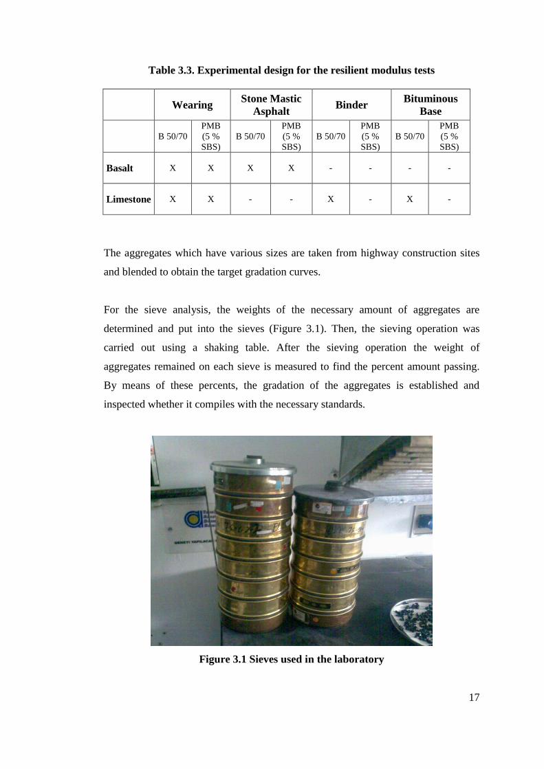
For the sieve analysis, the weights of the necessary amount of aggregates are
determined and put into the sieves (Figure 3.1). Then, the sieving operation was
carried out using a shaking table. After the sieving operation the weight of
aggregates remained on each sieve is measured to find the percent amount passing.
By means of these percents, the gradation of the aggregates is established and
inspected whether it compiles with the necessary standards.
Figure 3.1 Sieves used in the laboratory
18
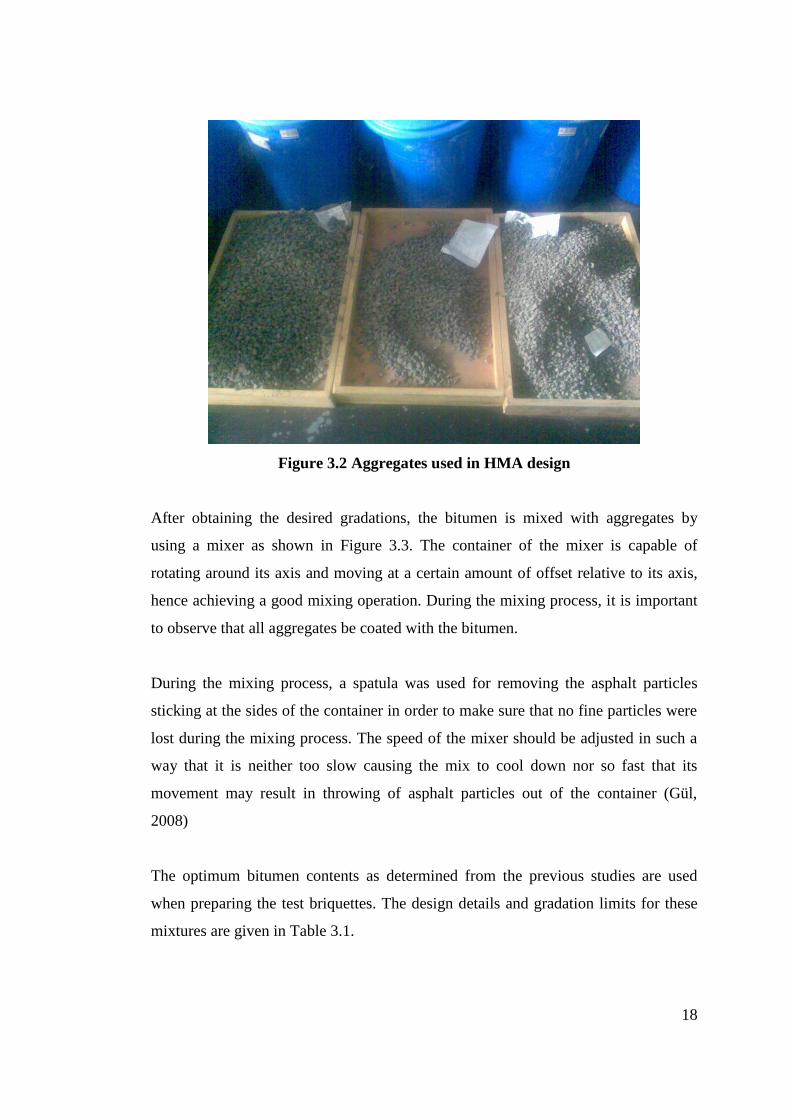
Figure 3.2 Aggregates used in HMA design
After obtaining the desired gradations, the bitumen is mixed with aggregates by
using a mixer as shown in Figure 3.3. The container of the mixer is capable of
rotating around its axis and moving at a certain amount of offset relative to its axis,
hence achieving a good mixing operation. During the mixing process, it is important
to observe that all aggregates be coated with the bitumen.
During the mixing process, a spatula was used for removing the asphalt particles
sticking at the sides of the container in order to make sure that no fine particles were
lost during the mixing process. The speed of the mixer should be adjusted in such a
way that it is neither too slow causing the mix to cool down nor so fast that its
movement may result in throwing of asphalt particles out of the container (Gül,
2008)
The optimum bitumen contents as determined from the previous studies are used
when preparing the test briquettes. The design details and gradation limits for these
mixtures are given in Table 3.1.
19
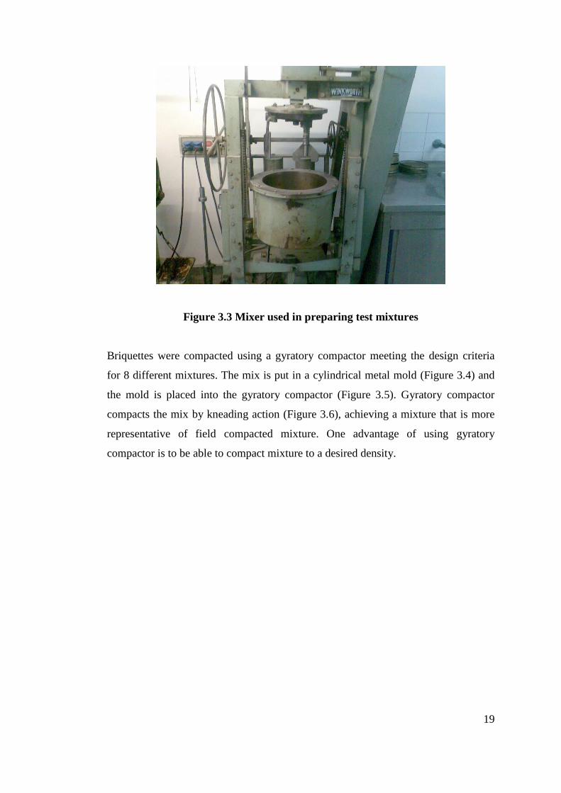
Figure 3.3 Mixer used in preparing test mixtures
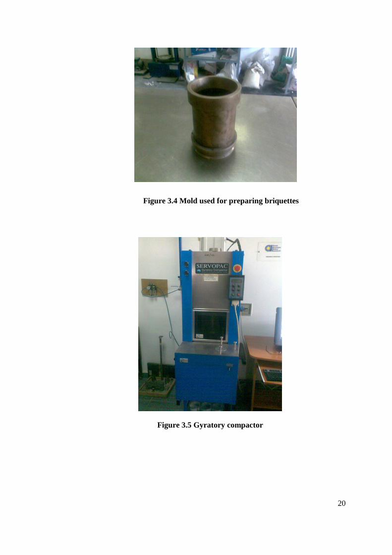
Briquettes were compacted using a gyratory compactor meeting the design criteria
for 8 different mixtures. The mix is put in a cylindrical metal mold (Figure 3.4) and
the mold is placed into the gyratory compactor (Figure 3.5). Gyratory compactor
compacts the mix by kneading action (Figure 3.6), achieving a mixture that is more
representative of field compacted mixture. One advantage of using gyratory
compactor is to be able to compact mixture to a desired density.
20
Figure 3.4 Mold used for preparing briquettes
Figure 3.5 Gyratory compactor
21
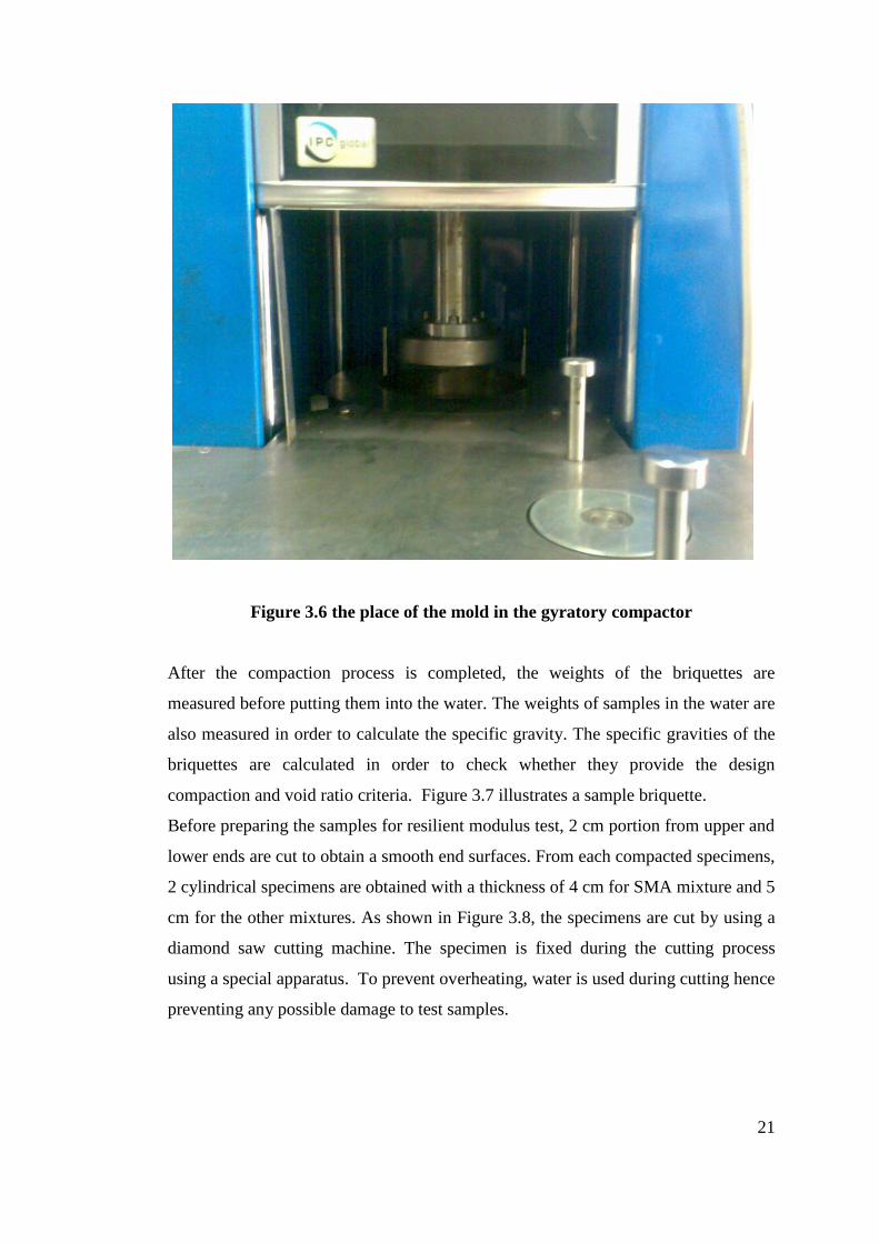
Figure 3.6 the place of the mold in the gyratory compactor
After the compaction process is completed, the weights of the briquettes are
measured before putting them into the water. The weights of samples in the water are
also measured in order to calculate the specific gravity. The specific gravities of the
briquettes are calculated in order to check whether they provide the design
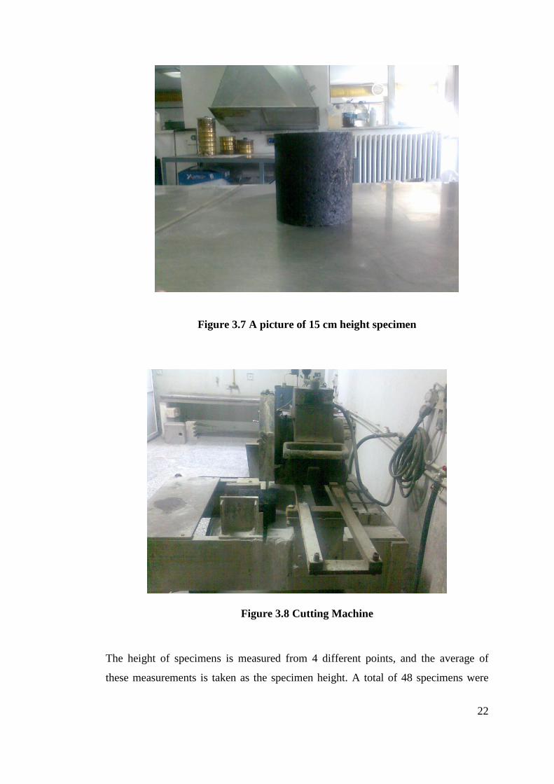
compaction and void ratio criteria. Figure 3.7 illustrates a sample briquette.
Before preparing the samples for resilient modulus test, 2 cm portion from upper and
lower ends are cut to obtain a smooth end surfaces. From each compacted specimens,
2 cylindrical specimens are obtained with a thickness of 4 cm for SMA mixture and 5
cm for the other mixtures. As shown in Figure 3.8, the specimens are cut by using a
diamond saw cutting machine. The specimen is fixed during the cutting process
using a special apparatus. To prevent overheating, water is used during cutting hence
preventing any possible damage to test samples.
22
Figure 3.7 A picture of 15 cm height specimen
Figure 3.8 Cutting Machine
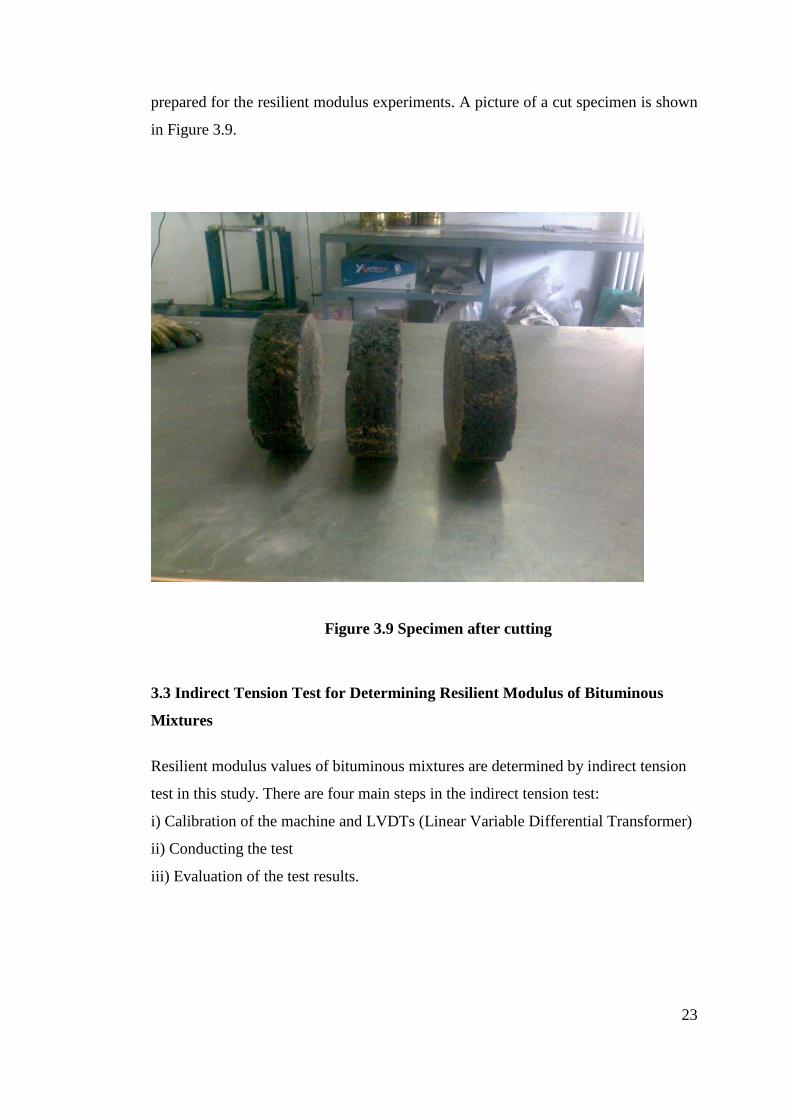
The height of specimens is measured from 4 different points, and the average of
these measurements is taken as the specimen height. A total of 48 specimens were
23
prepared for the resilient modulus experiments. A picture of a cut specimen is shown
in Figure 3.9.
Figure 3.9 Specimen after cutting
3.3 Indirect Tension Test for Determining Resilient Modulus of Bituminous
Mixtures
Resilient modulus values of bituminous mixtures are determined by indirect tension
test in this study. There are four main steps in the indirect tension test:
i) Calibration of the machine and LVDTs (Linear Variable Differential Transformer)
ii) Conducting the test
iii) Evaluation of the test results.
24
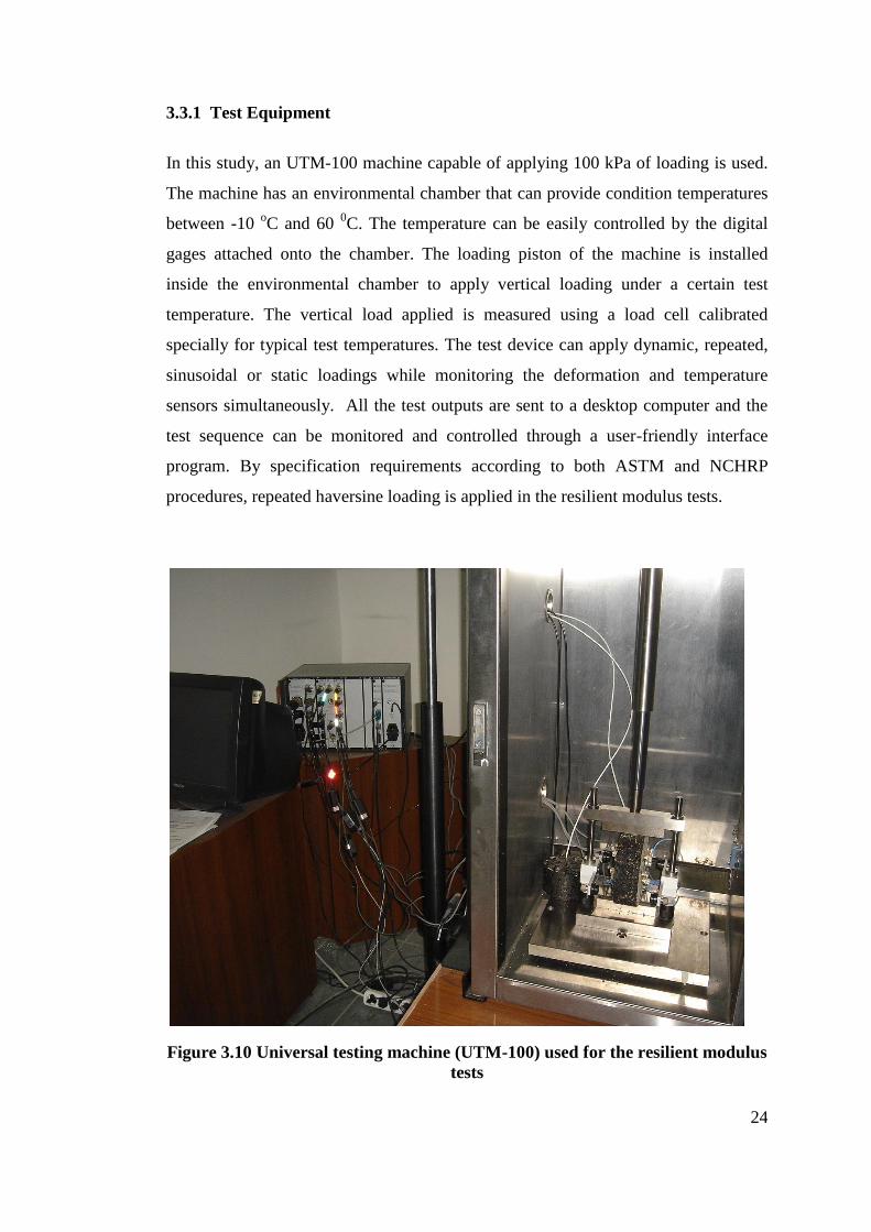
3.3.1 Test Equipment
In this study, an UTM-100 machine capable of applying 100 kPa of loading is used.
The machine has an environmental chamber that can provide condition temperatures
between -10 oC and 60
0C. The temperature can be easily controlled by the digital
gages attached onto the chamber. The loading piston of the machine is installed
inside the environmental chamber to apply vertical loading under a certain test
temperature. The vertical load applied is measured using a load cell calibrated
specially for typical test temperatures. The test device can apply dynamic, repeated,
sinusoidal or static loadings while monitoring the deformation and temperature
sensors simultaneously. All the test outputs are sent to a desktop computer and the
test sequence can be monitored and controlled through a user-friendly interface
program. By specification requirements according to both ASTM and NCHRP
procedures, repeated haversine loading is applied in the resilient modulus tests.
Figure 3.10 Universal testing machine (UTM-100) used for the resilient modulus
tests

25
3.3.2 Test Procedure
The resilient modulus test was conducted according to the NCHRP Project 1-28A
procedures “Laboratory Determination of Resilient Modulus for Flexible Pavement
Design”. In the testing process, first one of the specimens are chosen from each
layer and its indirect tension resistance is determined. The indirect tension resistance
test is performed by applying a vertical load at a rate of 50 mm/min according to
SHRP Protocol P07 “Test Method for Determining the Creep Compliance, Resilient
Modulus and Strength of Asphalt Materials Using the Indirect Tensile Test Device”.
The maximum load reached before the specimen starts to break is taken as the
indirect tension resistance.
After this operation, 3 specimens are chosen from each mixture for testing, On each
specimen surface, 4 small metallic LVDT installation fixtures (Figure 3.11-12) are
glued perpendicular to each other with 5 cm distance between them and left for
curing at least 6 hours. Then the horizontal and vertical LVDTs are installed through
the fixtures (Figure 3.13) and the specimen is placed into the testing device for
testing. The upper loading plate is placed onto the specimen and conditioned under
25 oC for 6 hours together with the test specimen. The test temperature is also
checked by the condition temperature of a dummy specimen located inside
environmental chamber.
Figure 3.11 Gluing of LVDT installation fixtures onto the test specimen by the
help of a mould

26
Figure 3.12 Installation fixtures glued onto the specimen
Figure 3.13 LVDTs installed on the specimen
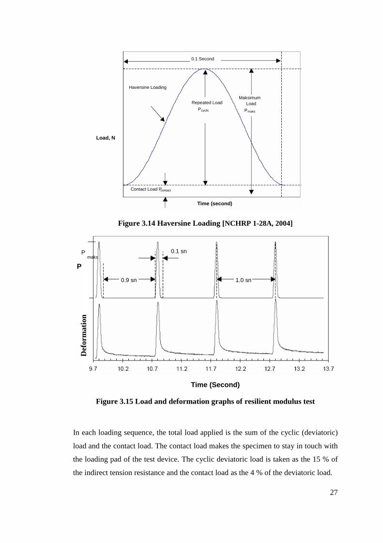
During the test, repeated haversine loading (Figure 3.14-3.15) is applied at 1 Hz to
the specimen with 0.1 sec loading and 0.9 sec rest period. After 100 conditioning
loadings, 5 loadings are applied and the average values of these loadings are taken as
the resilient modulus of the specimen under testing.
27
Figure 3.14 Haversine Loading [NCHRP 1-28A, 2004]
Figure 3.15 Load and deformation graphs of resilient modulus test
In each loading sequence, the total load applied is the sum of the cyclic (deviatoric)
load and the contact load. The contact load makes the specimen to stay in touch with
the loading pad of the test device. The cyclic deviatoric load is taken as the 15 % of
the indirect tension resistance and the contact load as the 4 % of the deviatoric load.
0.1 Second
Repeated Load P cyclic
Maksimum Load
P maks
Haversine Loading
Time (second)
Contact Load P contact
P
Def
orm
ati
on
0.1 sn
0.9 sn 1.0 sn
Time (Second)
P maks
Load, N
28
After completing the all loading sequences, the specimen is rotated 900
and the same
test sequence is applied one more time. The average of the resilient moduli
determined from these two steps is taken as the measured resilient modulus of test
specimen. Furthermore, the Poisson ratio of the specimen is established by using the
horizontal and vertical deformations.
The resilient modulus and the Poisson’s ratio are calculated by the user software
using the loading and the measured deformations during testing according to NCHRP
1-28A as follows:
Poisson Ratio:
h
v
h
v
δ
δ0.78010.3074
δ
δ0.23391.0695
μ
(3.1)
where;
µ : Poisson ratio
δv : Recoverable vertical deformation
δh : Recoverable horizontal deformation
Resilient Modulus:
)0.7801(0.2339t
PM
h
cyclic
R
(3.2)
where,
MR : Resilient modulus
δh : Recoverable horizontal deformation
29
Pcyclic : Applied cyclic deviatoric load (Pcyclic = Pmax – Pcontact)
Pmax : Applied maximum load
Pcontact : Contact load (Pmax*0.04)
t : Thickness of the specimen
µ : Poisson’s ratio
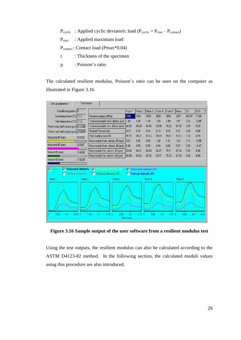
The calculated resilient modulus, Poisson’s ratio can be seen on the computer as
illustrated in Figure 3.16.
Figure 3.16 Sample output of the user software from a resilient modulus test
Using the test outputs, the resilient modulus can also be calculated according to the
ASTM D4123-82 method. In the following section, the calculated moduli values
using this procedure are also introduced.

30
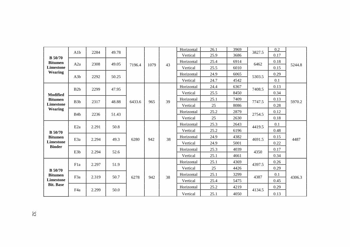
3.3.3 Test Results
According to NCHRP 1-28A
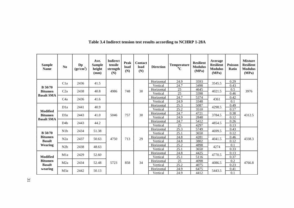
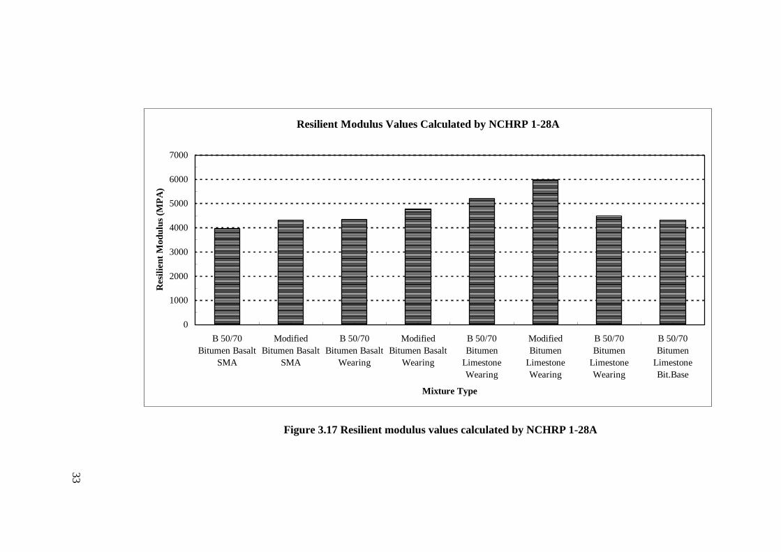
The results of resilient modulus test applied to 3 specimens from each mixture types
according to NCHRP 1-28A are given in Table 3.4 and Figure 3.17. In addition to
resilient modulus values, all Poisson’s ratios, maximum loads, and contact loads are
shown. Since the test is repeated after rotating the specimen 900, the results are given
both for horizontal and vertical position of the specimen. The resilient modulus of a
specimen is the average of the moduli calculated from vertical and horizontal
directions. Figure 3.18 illustrates the layer resilient modulus values.
31
Table 3.4 Indirect tension test results according to NCHRP 1-28A
Sample
Name No
Dp
(gr/cm3)
Ave.
Sample
height
(mm)
Indirect
tensile
strength
(N)
Peak
load
(N)
Contact
load
(N)
Direction Temperature
0C
Resilient
Modulus
(MPa)
Average
Resilient
Modulus
(MPa)
Poisson
Ratio
Mixture
Resilient
Modulus
(MPa)
B 50/70
Bitumen
Basalt SMA
C1a 2436 41.5
4986 748 30
Horizontal 24.9 3593 3545.5
0.29
3976
Vertical 24.7 3498 0.43
C2a 2438 40.8 Horizontal 25 4645
4021.5 0.5
Vertical 25 3398 0.46
C4a 2436 41.6 Horizontal 24.7 5374
4361 0.42
Vertical 24.9 3348 0.1
Modified
Bitumen
Basalt SMA
D1a 2441 40.9
5046 757 30
Horizontal 25.3 5087 4298.5
0.49
4312.5
Vertical 25.2 3510 0.17
D3a 2443 41.0 Horizontal 24.7 4721
3784.5 0.38
Vertical 24.9 2848 0.12
D4b 2443 44.2 Horizontal 24.7 5412
4854.5 0.26
Vertical 25 4297 0.13
B 50/70
Bitumen
Basalt
Wearing
N1b 2434 51.38
4750 713 29
Horizontal 25.3 5749 4699.5
0.43
4338.3
Vertical 25.1 3650 0.12
N2a 2437 50.63 Horizontal 24.8 4281
4041.5 0.46
Vertical 24.8 3802 0.12
N2b 2438 48.63 Horizontal 25.2 4898
4274 0.1
Vertical 25.1 3650 0.33
Modified
Bitumen
Basalt
wearing
M1a 2429 52.60
5723 858 34
Horizontal 24.8 4425 4770.5
0.13
4766.8
Vertical 25.1 5116 0.37
M2a 2434 52.48 Horizontal 25 4098
4086.5 0.2
Vertical 25.2 4075 0.23
M3a 2442 50.13 Horizontal 24.9 6475
5443.5 0.41
Vertical 24.9 4412 0.1
32
B 50/70
Bitumen
Limestone
Wearing
A1b 2284 49.78
7196.4 1079 43
Horizontal 26.1 3969 3827.5
0.2
5244.8
Vertical 25.9 3686 0.17
A2a 2308 49.05 Horizontal 25.4 6914
6462 0.18
Vertical 25.5 6010 0.15
A3b 2292 50.25 Horizontal 24.9 6065
5303.5 0.29
Vertical 24.7 4542 0.1
Modified
Bitumen
Limestone
Wearing
B2b 2299 47.95
6433.6 965 39
Horizontal 24.4 6367 7408.5
0.13
5970.2
Vertical 25.5 8450 0.34
B3b 2317 48.88 Horizontal 25.1 7409
7747.5 0.13
Vertical 25 8086 0.28
B4b 2236 51.43 Horizontal 25.2 2879
2754.5 0.12
Vertical 25 2630 0.18
B 50/70
Bitumen
Limestone
Binder
E2a 2.291 50.8
6280 942 38
Horizontal 25.3 2643 4419.5
0.1
4487
Vertical 25.2 6196 0.48
E3a 2.294 49.3 Horizontal 24.9 4382
4691.5 0.15
Vertical 24.9 5001 0.22
E3b 2.294 52.6 Horizontal 25.3 4039
4350 0.17
Vertical 25.1 4661 0.34
B 50/70
Bitumen
Limestone
Bit. Base
F1a 2.297 51.9
6278 942 38
Horizontal 25.1 4369 4397.5
0.26
4306.3
Vertical 25 4426 0.29
F3a 2.319 50.7 Horizontal 25.1 3299
4387 0.1
Vertical 25.4 5475 0.45
F4a 2.299 50.0 Horizontal 25.2 4219
4134.5 0.29
Vertical 25.1 4050 0.13
33
Resilient Modulus Values Calculated by NCHRP 1-28A
0
1000
2000
3000
4000
5000
6000
7000
B 50/70
Bitumen Basalt
SMA
Modified
Bitumen Basalt
SMA
B 50/70
Bitumen Basalt
Wearing
Modified
Bitumen Basalt
Wearing
B 50/70
Bitumen
Limestone
Wearing
Modified
Bitumen
Limestone
Wearing
B 50/70
Bitumen
Limestone
Wearing
B 50/70
Bitumen
Limestone
Bit.Base
Mixture Type
Resi
lien
t M
od
ulu
s (M
PA
)
Figure 3.17 Resilient modulus values calculated by NCHRP 1-28A
34
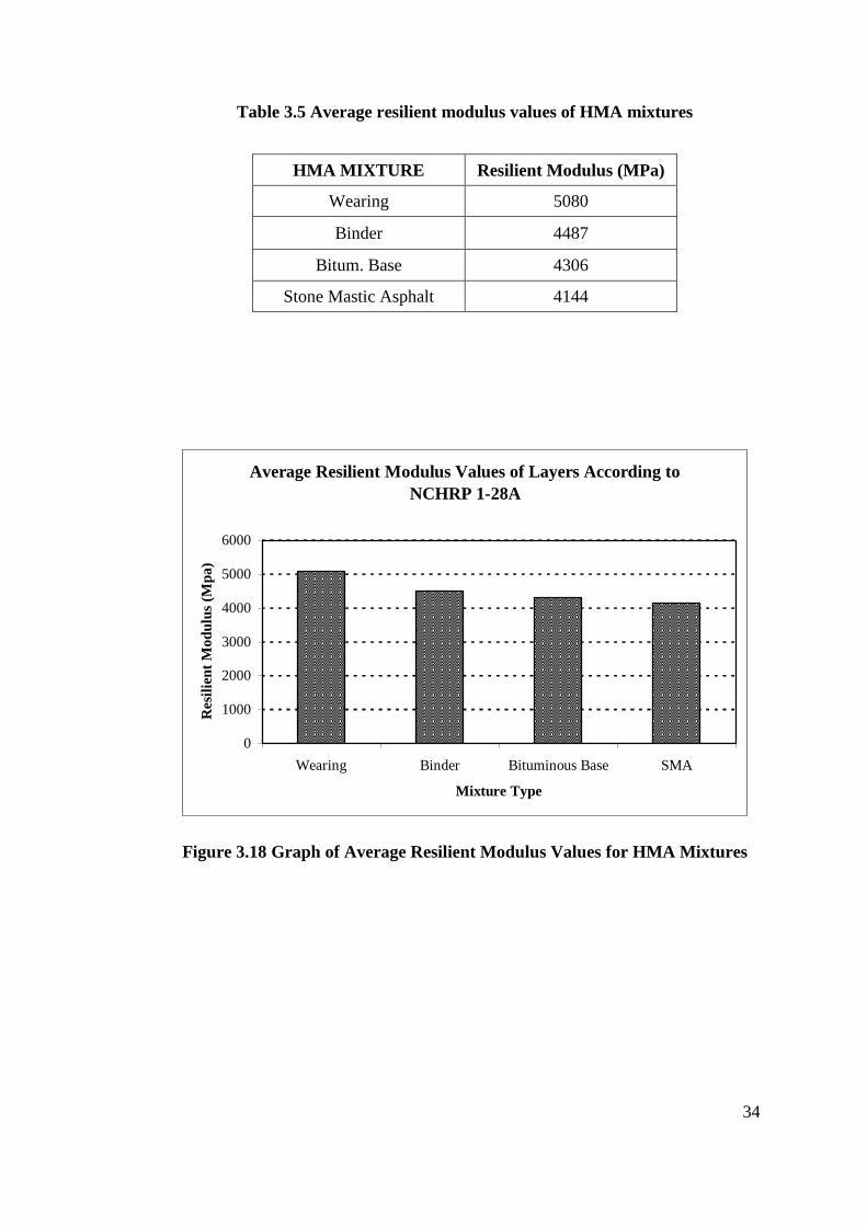
Table 3.5 Average resilient modulus values of HMA mixtures
Average Resilient Modulus Values of Layers According to
NCHRP 1-28A
0
1000
2000
3000
4000
5000
6000
Wearing Binder Bituminous Base SMA
Mixture Type
Resi
lien
t M
od
ulu
s (M
pa)
Figure 3.18 Graph of Average Resilient Modulus Values for HMA Mixtures
HMA MIXTURE Resilient Modulus (MPa)
Wearing 5080
Binder 4487
Bitum. Base 4306
Stone Mastic Asphalt 4144
35
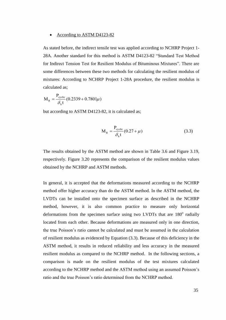
According to ASTM D4123-82
As stated before, the indirect tensile test was applied according to NCHRP Project 1-
28A. Another standard for this method is ASTM D4123-82 “Standard Test Method
for Indirect Tension Test for Resilient Modulus of Bituminous Mixtures”. There are
some differences between these two methods for calculating the resilient modulus of
mixtures: According to NCHRP Project 1-28A procedure, the resilient modulus is
calculated as;
)0.7801(0.2339t
PM
h
cyclic
R
but according to ASTM D4123-82, it is calculated as;
)(0.27t
PM
h
cyclic
R
(3.3)
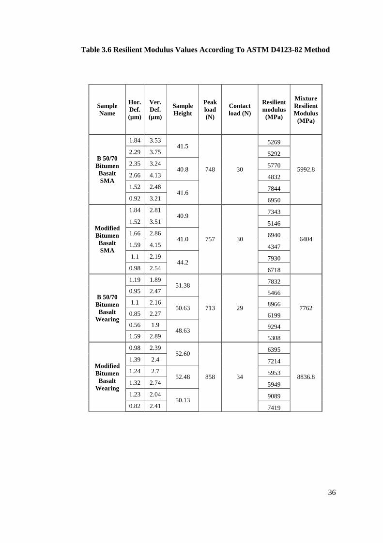
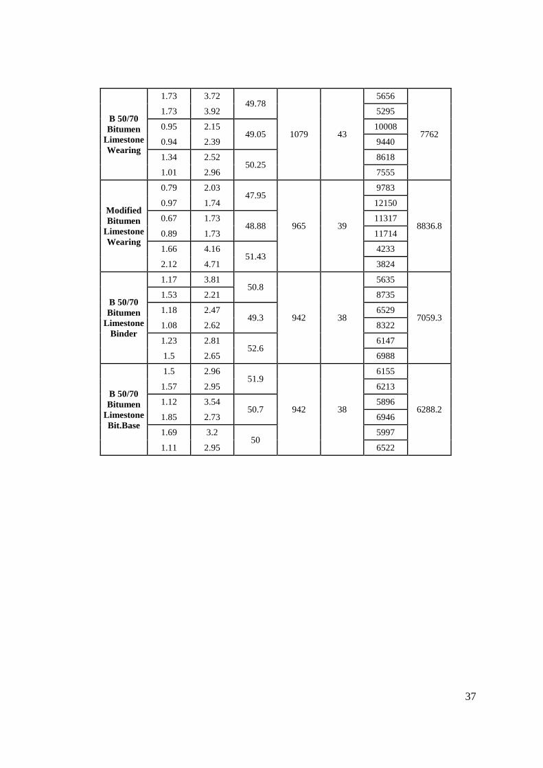
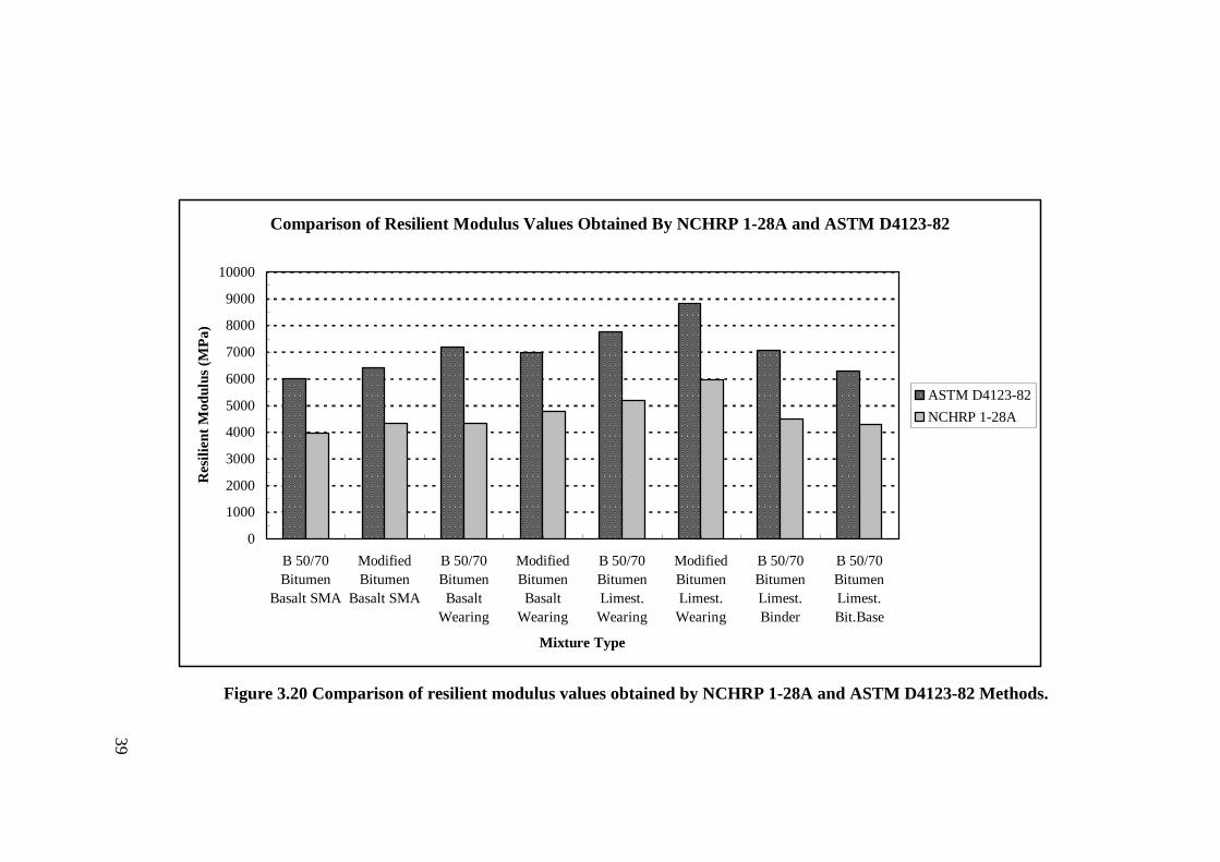
The results obtained by the ASTM method are shown in Table 3.6 and Figure 3.19,
respectively. Figure 3.20 represents the comparison of the resilient modulus values
obtained by the NCHRP and ASTM methods.
In general, it is accepted that the deformations measured according to the NCHRP
method offer higher accuracy than do the ASTM method. In the ASTM method, the
LVDTs can be installed onto the specimen surface as described in the NCHRP
method, however, it is also common practice to measure only horizontal
deformations from the specimen surface using two LVDTs that are 180o radially
located from each other. Because deformations are measured only in one direction,
the true Poisson’s ratio cannot be calculated and must be assumed in the calculation
of resilient modulus as evidenced by Equation (3.3). Because of this deficiency in the
ASTM method, it results in reduced reliability and less accuracy in the measured
resilient modulus as compared to the NCHRP method. In the following sections, a
comparison is made on the resilient modulus of the test mixtures calculated
according to the NCHRP method and the ASTM method using an assumed Poisson’s
ratio and the true Poisson’s ratio determined from the NCHRP method.
36
Table 3.6 Resilient Modulus Values According To ASTM D4123-82 Method
Sample
Name
Hor.
Def.
(µm)
Ver.
Def.
(µm)
Sample
Height
Peak
load
(N)
Contact
load (N)
Resilient
modulus
(MPa)
Mixture
Resilient
Modulus
(MPa)
B 50/70
Bitumen
Basalt
SMA
1.84 3.53 41.5
748 30
5269
5992.8
2.29 3.75 5292
2.35 3.24 40.8
5770
2.66 4.13 4832
1.52 2.48 41.6
7844
0.92 3.21 6950
Modified
Bitumen
Basalt
SMA
1.84 2.81 40.9
757 30
7343
6404
1.52 3.51 5146
1.66 2.86 41.0
6940
1.59 4.15 4347
1.1 2.19 44.2
7930
0.98 2.54 6718
B 50/70
Bitumen
Basalt
Wearing
1.19 1.89 51.38
713 29
7832
7762
0.95 2.47 5466
1.1 2.16 50.63
8966
0.85 2.27 6199
0.56 1.9 48.63
9294
1.59 2.89 5308
Modified
Bitumen
Basalt
Wearing
0.98 2.39 52.60
858 34
6395
8836.8
1.39 2.4 7214
1.24 2.7 52.48
5953
1.32 2.74 5949
1.23 2.04 50.13
9089
0.82 2.41 7419
37
B 50/70
Bitumen
Limestone
Wearing
1.73 3.72 49.78
1079 43
5656
7762
1.73 3.92 5295
0.95 2.15 49.05
10008
0.94 2.39 9440
1.34 2.52 50.25
8618
1.01 2.96 7555
Modified
Bitumen
Limestone
Wearing
0.79 2.03 47.95
965 39
9783
8836.8
0.97 1.74 12150
0.67 1.73 48.88
11317
0.89 1.73 11714
1.66 4.16 51.43
4233
2.12 4.71 3824
B 50/70
Bitumen
Limestone
Binder
1.17 3.81 50.8
942 38
5635
7059.3
1.53 2.21 8735
1.18 2.47 49.3
6529
1.08 2.62 8322
1.23 2.81 52.6
6147
1.5 2.65 6988
B 50/70
Bitumen
Limestone
Bit.Base
1.5 2.96 51.9
942 38
6155
6288.2
1.57 2.95 6213
1.12 3.54 50.7
5896
1.85 2.73 6946
1.69 3.2 50
5997
1.11 2.95 6522

38
Resilient Modulus Values Calculated According to ASTM D4123-82
0
1000
2000
3000
4000
5000
6000
7000
8000
9000
10000
B 50/70
Bitumen Basalt
SMA
Modified
Bitumen
Basalt SMA
B 50/70
Bitumen Basalt
Wearing
Modified
Bitumen
Basalt Wearing
B 50/70
Bitumen
Limestone
Wearing
Modified
Bitumen
Limestone
Wearing
B 50/70
Bitumen
Limestone
Binder
B 50/70
Bitumen
Limestone
Bit.Base
Mixture Type
Resi
lien
t M
od
ulu
s (M
Pa)
Figure 3.19 Graph of resilient modulus values according to ASTM D4123-82 Method.
39
Comparison of Resilient Modulus Values Obtained By NCHRP 1-28A and ASTM D4123-82
0
1000
2000
3000
4000
5000
6000
7000
8000
9000
10000
B 50/70
Bitumen
Basalt SMA
Modified
Bitumen
Basalt SMA
B 50/70
Bitumen
Basalt
Wearing
Modified
Bitumen
Basalt
Wearing
B 50/70
Bitumen
Limest.
Wearing
Modified
Bitumen
Limest.
Wearing
B 50/70
Bitumen
Limest.
Binder
B 50/70
Bitumen
Limest.
Bit.Base
Mixture Type
Resi
lien
t M
od
ulu
s (M
Pa)
ASTM D4123-82
NCHRP 1-28A
Figure 3.20 Comparison of resilient modulus values obtained by NCHRP 1-28A and ASTM D4123-82 Methods.
40
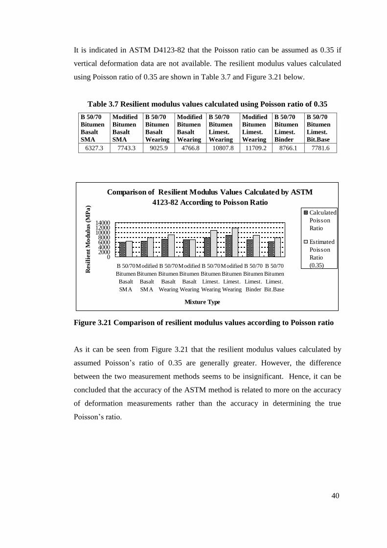
It is indicated in ASTM D4123-82 that the Poisson ratio can be assumed as 0.35 if
vertical deformation data are not available. The resilient modulus values calculated
using Poisson ratio of 0.35 are shown in Table 3.7 and Figure 3.21 below.
Table 3.7 Resilient modulus values calculated using Poisson ratio of 0.35
B 50/70
Bitumen
Basalt
SMA
Modified
Bitumen
Basalt
SMA
B 50/70
Bitumen
Basalt
Wearing
Modified
Bitumen
Basalt
Wearing
B 50/70
Bitumen
Limest.
Wearing
Modified
Bitumen
Limest.
Wearing
B 50/70
Bitumen
Limest.
Binder
B 50/70
Bitumen
Limest.
Bit.Base
6327.3 7743.3 9025.9 4766.8 10807.8 11709.2 8766.1 7781.6
Comparison of Resilient Modulus Values Calculated by ASTM
4123-82 According to Poisson Ratio
02000400060008000
100001200014000
B 50/70
Bitumen
Basalt
SMA
Modified
Bitumen
Basalt
SMA
B 50/70
Bitumen
Basalt
Wearing
Modified
Bitumen
Basalt
Wearing
B 50/70
Bitumen
Limest.
Wearing
Modified
Bitumen
Limest.
Wearing
B 50/70
Bitumen
Limest.
Binder
B 50/70
Bitumen
Limest.
Bit.Base
Mixture Type
Resi
lien
t M
od
ulu
s (M
Pa
)
Calculated
Poisson
Ratio
Estimated
Poisson
Ratio
(0.35)
Figure 3.21 Comparison of resilient modulus values according to Poisson ratio
As it can be seen from Figure 3.21 that the resilient modulus values calculated by
assumed Poisson’s ratio of 0.35 are generally greater. However, the difference
between the two measurement methods seems to be insignificant. Hence, it can be
concluded that the accuracy of the ASTM method is related to more on the accuracy
of deformation measurements rather than the accuracy in determining the true
Poisson’s ratio.
41
CHAPTER 4
DETERMINATION OF RESILIENT MODULUS BY NOMOGRAPHS AND E
EMPIRICAL EQUATIONS
In this chapter, methods for determining resilient modulus of bituminous mixtures
are presented using nomographs and various empirical equations that have still been
in pavement design procedures. The methods generally use binder and aggregate
stiffness properties to calculate the resilient modulus of bituminous mixtures. In the
below sections, moduli values calculated using various methods are compared.
4.1 Van Der Poel and Shell Nomographs
4.1.1 Van Der Poel Nomograph
Van Der Poel Nomograph, as described in Section 2.4, is used to estimate the
bitumen stiffness. The parameters needed to estimate the stiffness of bitumen from
the Van Der Poel Nomograph are:
i) For B50/70 Bitumen;
TRB=48.8 0C
T = 25 0C
T- TRB = 23.8 0C
Time of Loading = 0.1 seconds
Sb = 4.5 x 10⁶ N/m
2 (estimated from the nomograph)
046.08.4825
)800log()
log(63A
96.0
50x0.0461
500x0.046-20PI
42
ii) For 5% SBS Modified Bitumen
TRB=81.2 0C
T = 25 0C
T- TRB = 56.2 0C
PI = 4.26 (Calculated)
Time of Loading = 0.1 seconds
Sb = 4 x 10⁶ N/m
2 (estimated from the nomograph)
4.1.2 Shell Nomograph
The stiffness of the bitumen was estimated as 4.5x10⁶
Pa and 4x10⁶ Pa, but in this
study for Shell nomograph, the values are assumed as 5x10⁶ Pa. In order to estimate
the resilient modulus from the Shell nomograph, the percent volume of bitumen and
aggregate is needed. The calculations for SMA prepared by B 50/70 bitumen and
basalt are shown below. The results for the other mixtures and graph of the results
are given in Table 4.1. and Figure 3.19, respectively.
Sb = 5 x10⁶ N/m
2
70.1402.1
)458.2061.0(100
xxbV
77.8182.2
458.2)061.01(100
xxgV
Smix = 1000 MPa
022.02.8125
)800log()
log(46A
26.4
50x0.0221
500x0.022-20PI

43
Table 4.1 The resilient modulus of the mixtures estimated by Shell Nomograph
Bazalt Limestone
SMA Wearing Wearing Binder Bitum.
Base
50/70 PMB 50/70 PMB 50/70 PMB 50/70 50/70
Vg 81.76 81.76 83.22 83.22 84.46 84.46 84.82 84.79
Vb 14.70 14.70 12.12 12.12 11.55 11.55 11.01 9.90
Sb 5x10⁶
5x10⁶ 5x10
6 5x10
6 5x10
6 5x10
6 5x10
6 5x10
6
Smix 1000 1000 1300 1300 1400 1400 1600 1650

44
Resilient Modulus Values Estimated by Shell Nomograph
0
300
600
900
1200
1500
1800
B 50/70 Bitumen
Basalt SMA
Modified
Bitumen Basalt
SMA
B 50/70 Bitumen
Basalt Wearing
Modified
Bitumen Basalt
Wearing
B 50/70 Bitumen
Limestone
Wearing
Modified
Bitumen
Limestone
Wearing
B 50/70 Bitumen
Limestone Binder
B 50/70 Bitumen
Limestone
Bit.Base
Mixture Type
Resi
lien
t M
od
ulu
s (M
pa
)
Figure 4.1 Graph of the resilient modulus values calculated by Shell Nomograph (1977).
45
4.2 Estimation of the Stiffness Modulus of Mixtures by Empirical Equations
Resilient modulus values can be estimated by various empirical equations. For,
some of these equations, the stiffness of bitumen should be determined first. Hence, a
description of the method to estimate the bitumen stiffness is given first , and then
the estimation of resilient modulus using bitumen stiffness, aggregate and bitumen
characteristics are explained based on various empirical methods.
4.2.1 Estimation of Bitumen Stiffness by Empirical Equations
The stiffness of the bitumen can be estimated by the Van Der Poel equation as stated
in the previous sections.
57 )10157.1 Te PI
RB
-0.368
wb (Tt S
The determined values by Van Der Poel equation for B50/70 bitumen are given
below:
i) For B50/70 bitumen
596.07 )251.010157.1 (48.8 S -0.368
b e
Sb = 5.39 x 10⁶ MPa
ii) For Modified Bitumen
526.47 )251.010157.1 (81.2 S -0.368
b e
Sb = 2.13 x 10⁶ MPa
4.2.2 Estimation of the Resilient Modulus of Mixtures By Empirical Equations
The stiffness modulus of the bitumen is calculated by Bonnaure et al. (1977),
Heukelom and Klomp (1964) and Witczak predictive equations (2000) as explained
in the previous chapters.

46
Bonnaure et al. (1977) Equation :
The estimation of stiffness for SMA prepared with basalt and B 50/70 bitumen are
shown below. The remaining results are shown in Table 4.2 and Figure 4.2 shows the
graph of the results. Vg and Vb values are taken as 81.77 and 14.70, respectively
which were calculated by Equation 2.6 and 2.7.
566.1070.1477.81
)82,101
81.77-1,342(100
892.977.810002135,077.810568,00,8 2
2 xx
721.0170.1433,1
)1log(6,03
x
21,37x14.70
512.0)892.9566.10(7582,04
the stiffness of the bitumen is assumed as 5x10⁶ MPa.
892.98105log2
721.0512.0)8105(log
2
721.0566.10log 66
xxSm
954.8log mS
72.898mS MPa
Since the stiffness of the bitumen for B 50/70 and PMB are assumed to be equal, the
mixture stiffness values turn out to be equal for the mixtures prepared with different
types of bitumen.
47
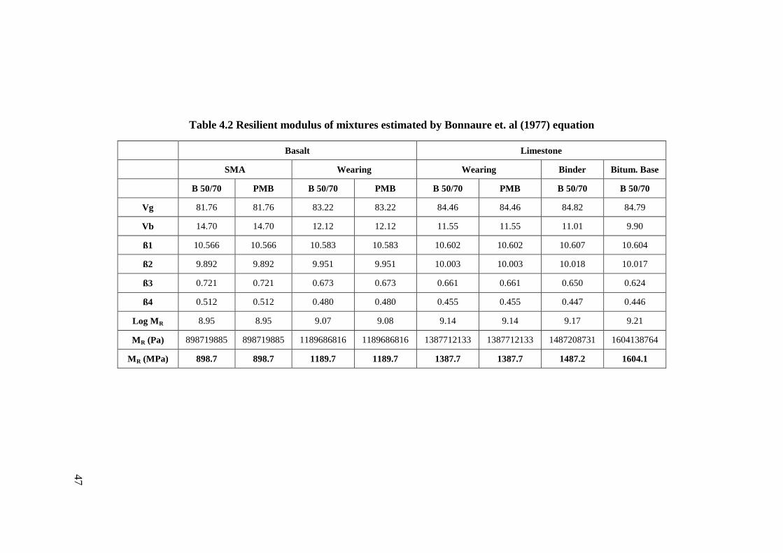
Table 4.2 Resilient modulus of mixtures estimated by Bonnaure et. al (1977) equation
Basalt Limestone
SMA Wearing Wearing Binder Bitum. Base
B 50/70 PMB B 50/70 PMB B 50/70 PMB B 50/70 B 50/70
Vg 81.76 81.76 83.22 83.22 84.46 84.46 84.82 84.79
Vb 14.70 14.70 12.12 12.12 11.55 11.55 11.01 9.90
ß1 10.566 10.566 10.583 10.583 10.602 10.602 10.607 10.604
ß2 9.892 9.892 9.951 9.951 10.003 10.003 10.018 10.017
ß3 0.721 0.721 0.673 0.673 0.661 0.661 0.650 0.624
ß4 0.512 0.512 0.480 0.480 0.455 0.455 0.447 0.446
Log MR 8.95 8.95 9.07 9.08 9.14 9.14 9.17 9.21
MR (Pa) 898719885 898719885 1189686816 1189686816 1387712133 1387712133 1487208731 1604138764
MR (MPa) 898.7 898.7 1189.7 1189.7 1387.7 1387.7 1487.2 1604.1
48
Resilient Modulus Values Estimated by Bonnaure et al. Equation (1977)
0
300
600
900
1200
1500
1800
B 50/70
Bitumen Basalt
SMA
Modified
Bitumen Basalt
SMA
B 50/70
Bitumen Basalt
Wearing
Modified
Bitumen Basalt
Wearing
B 50/70
Bitumen
Limestone
Wearing
Modified
Bitumen
Limestone
Wearing
B 50/70
Bitumen
Limestone
Binder
B 50/70
Bitumen
Limestone
Bit.Base
Mixture Type
Resi
lien
t M
od
ulu
s (M
pa)
Figure 4.2 Graph of the resilient modulus values calculated by Bonnaure et. al (1977) Equation.
49
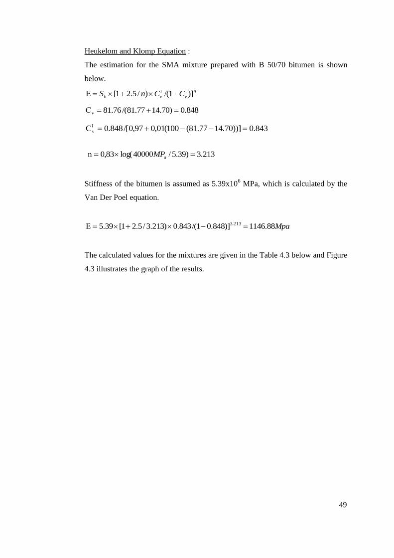
Heukelom and Klomp Equation :
The estimation for the SMA mixture prepared with B 50/70 bitumen is shown
below.
n
v
ı
vb CCnS )]1/()/5.21[ E
848.0)70.1477.81/(76.81 vC
213.3)39.5/40000log(83,0 aMPn
Stiffness of the bitumen is assumed as 5.39x10⁶ MPa, which is calculated by the
Van Der Poel equation.
Mpa88.1146)]848.01/(843.0)213.3/5.21[39.5 213.3 E
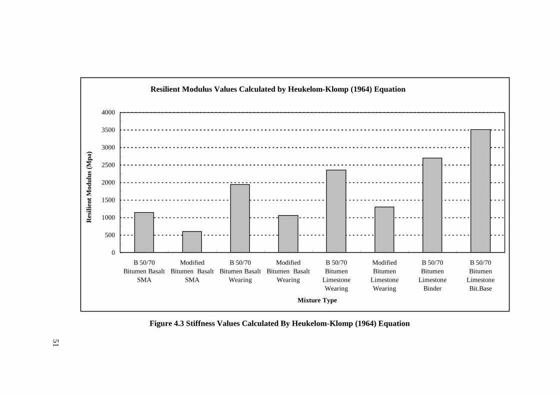
The calculated values for the mixtures are given in the Table 4.3 below and Figure
4.3 illustrates the graph of the results.
843.0))]70.1477.81(100(01,097,0/[848.0 1
vC
50
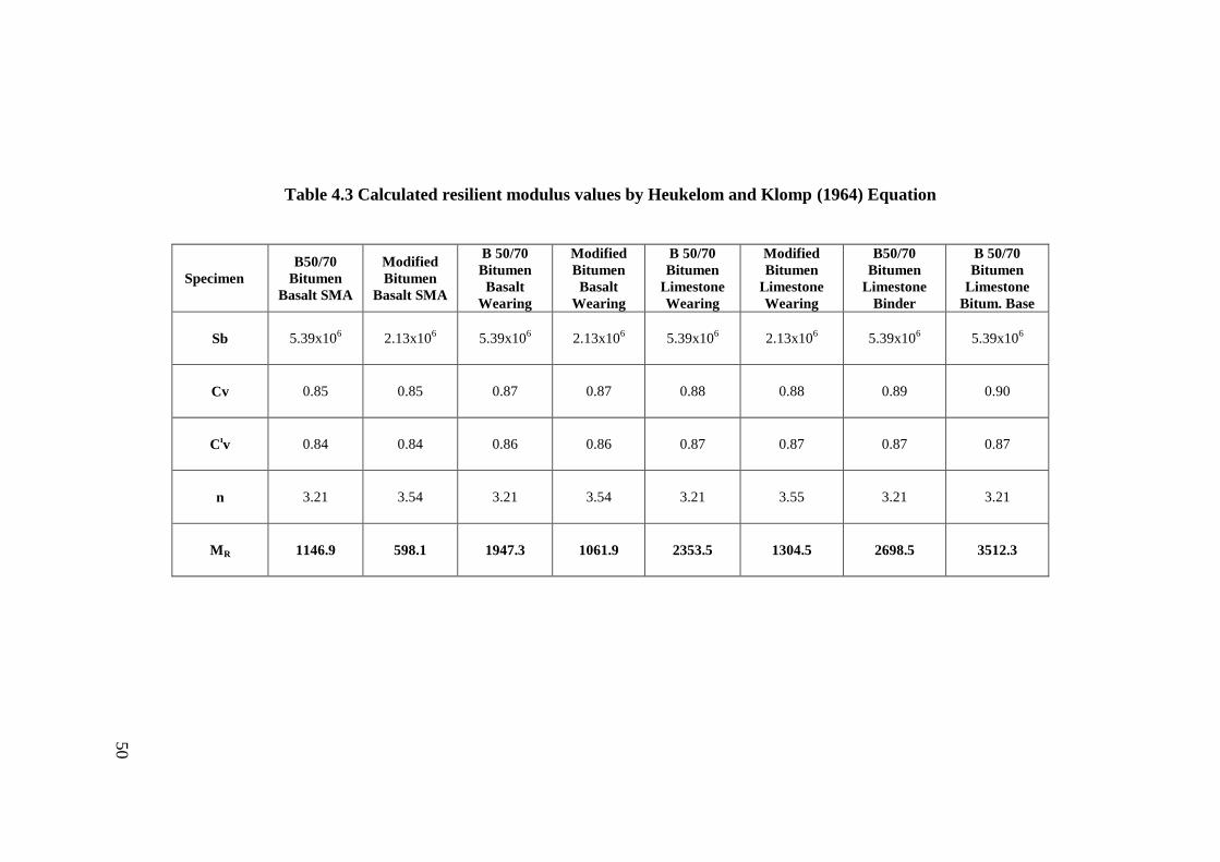
Table 4.3 Calculated resilient modulus values by Heukelom and Klomp (1964) Equation
Specimen
B50/70
Bitumen
Basalt SMA
Modified
Bitumen
Basalt SMA
B 50/70
Bitumen
Basalt
Wearing
Modified
Bitumen
Basalt
Wearing
B 50/70
Bitumen
Limestone
Wearing
Modified
Bitumen
Limestone
Wearing
B50/70
Bitumen
Limestone
Binder
B 50/70
Bitumen
Limestone
Bitum. Base
Sb 5.39x10⁶ 2.13x10
6 5.39x10
6 2.13x10
6 5.39x10
6 2.13x10
6 5.39x10
6 5.39x10
6
Cv 0.85 0.85 0.87 0.87 0.88 0.88 0.89 0.90
Cıv 0.84 0.84 0.86 0.86 0.87 0.87 0.87 0.87
n 3.21 3.54 3.21 3.54 3.21 3.55 3.21 3.21
MR 1146.9 598.1 1947.3 1061.9 2353.5 1304.5 2698.5 3512.3
51
Resilient Modulus Values Calculated by Heukelom-Klomp (1964) Equation
0
500
1000
1500
2000
2500
3000
3500
4000
B 50/70
Bitumen Basalt
SMA
Modified
Bitumen Basalt
SMA
B 50/70
Bitumen Basalt
Wearing
Modified
Bitumen Basalt
Wearing
B 50/70
Bitumen
Limestone
Wearing
Modified
Bitumen
Limestone
Wearing
B 50/70
Bitumen
Limestone
Binder
B 50/70
Bitumen
Limestone
Bit.Base
Mixture Type
Resi
lien
t M
od
ulu
s (M
pa
)
Figure 4.3 Stiffness Values Calculated By Heukelom-Klomp (1964) Equation
52
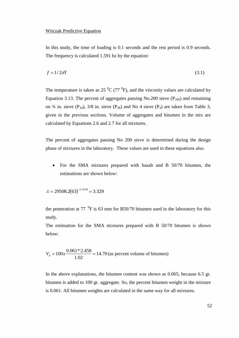
Witczak Predictive Equation
In this study, the time of loading is 0.1 seconds and the rest period is 0.9 seconds.
The frequency is calculated 1.591 hz by the equation:
2/1f (3.1)
The temperature is taken as 25 0C (77
0F), and the viscosity values are calculated by
Equation 3.13. The percent of aggregates passing No.200 sieve (P200) and remaining
on ¾ in. sieve (P34), 3/8 in. sieve (P38) and No 4 sieve (P4) are taken from Table 3,
given in the previous sections. Volume of aggregates and bitumen in the mix are
calculated by Equations 2.6 and 2.7 for all mixtures.
The percent of aggregates passing No 200 sieve is determined during the design
phase of mixtures in the laboratory. These values are used in these equations also.
For the SMA mixtures prepared with basalt and B 50/70 bitumen, the
estimations are shown below:
329.3632.295081939.2
the penetration at 77 0
F is 63 mm for B50/70 bitumen used in the laboratory for this
study.
The estimation for the SMA mixtures prepared with B 50/70 bitumen is shown
below:
70.1402.1
458.2*061.0100 xVb (as percent volume of bitumen)
In the above explanations, the bitumen content was shown as 0.065, because 6.5 gr.
bitumen is added to 100 gr. aggregate. So, the percent bitumen weight in the mixture
is 0.061. All bitumen weights are calculated in the same way for all mixtures.
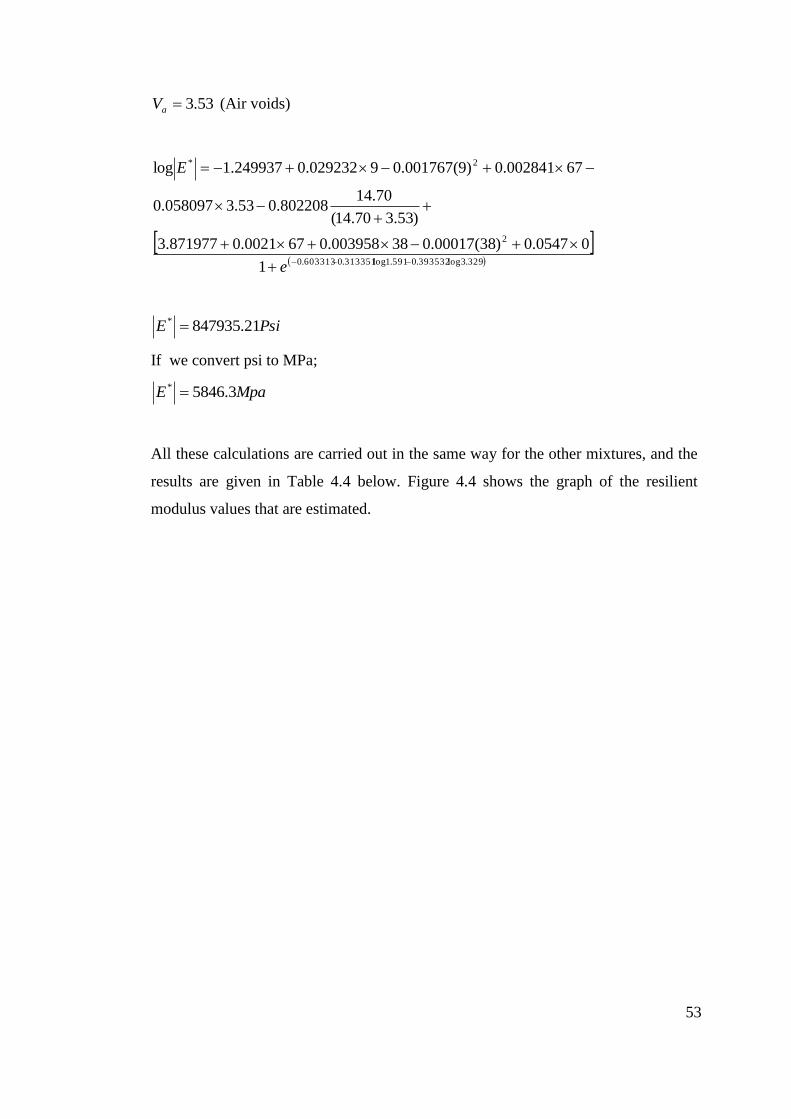
53
53.3aV (Air voids)
329.3log393532.0591.1log313351.0603313.0
2
2*
1
00547.0)38(00017.038003958.0670021.0871977.3
)53.370.14(
70.14802208.053.3058097.0
67002841.0)9(001767.09029232.0249937.1log
e
E
PsiE 21.847935*
If we convert psi to MPa;
MpaE 3.5846*
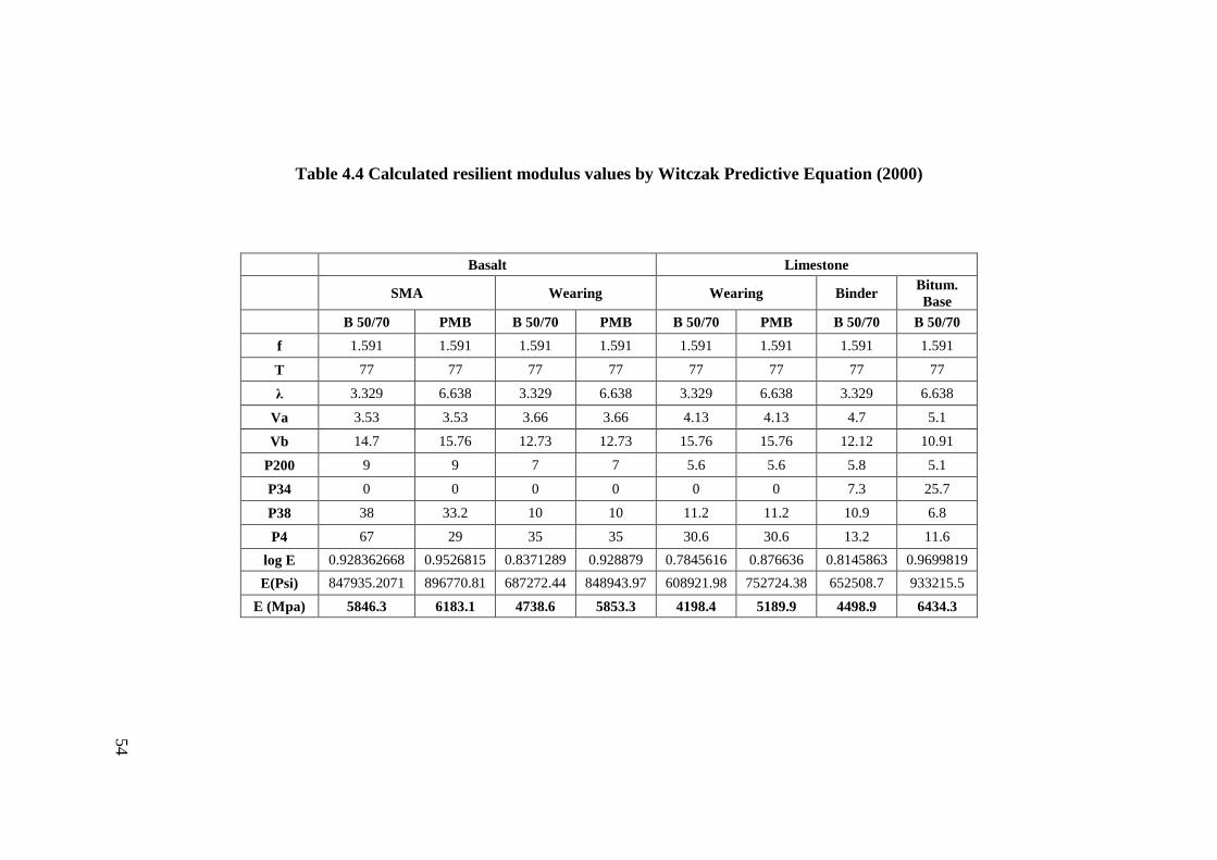
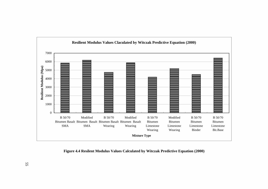
All these calculations are carried out in the same way for the other mixtures, and the
results are given in Table 4.4 below. Figure 4.4 shows the graph of the resilient
modulus values that are estimated.
54
Table 4.4 Calculated resilient modulus values by Witczak Predictive Equation (2000)
Basalt Limestone
SMA Wearing Wearing Binder Bitum.
Base
B 50/70 PMB B 50/70 PMB B 50/70 PMB B 50/70 B 50/70
f 1.591 1.591 1.591 1.591 1.591 1.591 1.591 1.591
T 77 77 77 77 77 77 77 77
λ 3.329 6.638 3.329 6.638 3.329 6.638 3.329 6.638
Va 3.53 3.53 3.66 3.66 4.13 4.13 4.7 5.1
Vb 14.7 15.76 12.73 12.73 15.76 15.76 12.12 10.91
P200 9 9 7 7 5.6 5.6 5.8 5.1
P34 0 0 0 0 0 0 7.3 25.7
P38 38 33.2 10 10 11.2 11.2 10.9 6.8
P4 67 29 35 35 30.6 30.6 13.2 11.6
log E 0.928362668 0.9526815 0.8371289 0.928879 0.7845616 0.876636 0.8145863 0.9699819
E(Psi) 847935.2071 896770.81 687272.44 848943.97 608921.98 752724.38 652508.7 933215.5
E (Mpa) 5846.3 6183.1 4738.6 5853.3 4198.4 5189.9 4498.9 6434.3
55
Resilient Modulus Values Claculated by Witczak Predictive Equation (2000)
0
1000
2000
3000
4000
5000
6000
7000
B 50/70
Bitumen Basalt
SMA
Modified
Bitumen Basalt
SMA
B 50/70
Bitumen Basalt
Wearing
Modified
Bitumen Basalt
Wearing
B 50/70
Bitumen
Limestone
Wearing
Modified
Bitumen
Limestone
Wearing
B 50/70
Bitumen
Limestone
Binder
B 50/70
Bitumen
Limestone
Bit.Base
Mixture Type
Resi
lien
t M
od
ulu
s (M
pa
)
Figure 4.4 Resilent Modulus Values Calculated by Witczak Predictive Equation (2000)
56
4.2.3 Discussion of Results
In this section, comparison of the empirical estimation methods is presented in two
stages. The predicted modulus values are first compared with results of two
measurement methods. In the second stage, relative errors are calculated for each
estimation method with respect to the measured values. A discussion is also given
for the strength of empirical models to approximate the actual modulus values.
- Comparison of Results between ASTM and NCHRP Methods
Comparison of resilient modulus values based on the ASTM and NCHRP methods
are shown in Figure 4.5. It can be seen that the moduli determined according to the
ASTM method are always higher than those based on the NCHRP method. It is also
interesting to note that the largest differences are obtained for wearing course
mixtures. While the smallest differences are obtained from the SMA mixtures, the
binder course mixtures seem to fall between these categories. It should be
remembered that the ASTM values are obtained using the deformation measurements
from the NCHRP method and the only difference between the two results is the
method of calculation of resilient moduli values. Based on these outcomes, the SMA
mixtures seem to have less sensitivity to the calculated resilient modulus values as
compared to the other mixtures. On the other hand, the wearing course mixtures
show the highest sensitivity to the methods used. The reason that the ASTM method
produces always higher modulus can be related to either the accuracy level in the
calibration of the model to calculate resilient modulus or the assumed Poisson’s ratio
effect, which should be verified using a larger experimental data.

57
0
2000
4000
6000
8000
10000
B 50/70
Bitumen
Basalt SMA
Modified
Bitumen
Basalt SMA
B 50/70
Bitumen
Basalt
Wearing
Modified
Bitumen
Basalt
Wearing
B 50/70
Bitumen
Limestone
Wearing
Modified
Bitumen
Limestone
Wearing
B 50/70
Bitumen
Limestone
Binder
B 50/70
Bitumen
Limestone
Bitum. Base
Resi
lien
t M
od
ulu
s (M
Pa
)
ASTM D4123-82
NCHRP 1-28A
Figure 4.5 Comparison of resilient modulus values based on ASTM and
NCHRP methods
- Comparison of Results between Empirical Methods
The estimated resilient modulus values are given in Table 4.5 for each empirical
methods together with the ASTM and NCHRP results. The data are also presented in
Figure 4.6 to compare between the estimation methods. It can be seen that the
ASTM methods again produces the highest modulus values among the other
estimation methods. The Witczak (2000) predictive equation, on the other hand,
yields the next highest estimation of modulus values followed by results of the
NCHRP method. The other estimation methods, i.e., Heukelom-Klomp (1964), Shell
(1954) and the Bonnaure et. al (1977), give lower values as compared to the other
methods as can be observed from Figure 4.6.
The comparison of the empirical methods are also given separately for the ASTM
and the NCHRP methods using an error coefficient, e, as in Table 4.6 and 4.7.
1
21100E
EExe
(4.1)
58
where.
e = percent error (%),
E1 = resilient modulus values measured in Laboratory by Indirect Tension Test,
E2 = estimated resilient modulus value estimated by other methods.
Because the ASTM methods gives the highest modulus values, the percent errors
calculated for each empirical methods according to Equation (4.1) are higher as
compare to the NCHRP method. It can be seen that the largest error is obtained from
the Bonnaure (1977) method with 73.68% error for the NCHRP method while
83.25% for the ASTM method. The Shell (1954) and the Heukelom-Klomp (1964)
methods produce the next highest errors after the Bonnaure (1977) method. As
stated earlier, the smallest error is obtained from the Witczak (2000) predictive
equation with an average error of 17.38 % for the NCHRP and 24.71% for the
ASTM method. As can be seen from Figure 4.7, the Witczak (2000) method was
found to produce results that are closest to both measurement methods with an
average error of not more than 25%. Based on these results, it can be recommended
that if a laboratory measured resilient modulus is not available; the Witczak (2000)
predictive equation should be used among the other estimation methods to predict the
actual modulus. However, because the data presented in this study are quite limited,
these results should be supported using larger data sets.
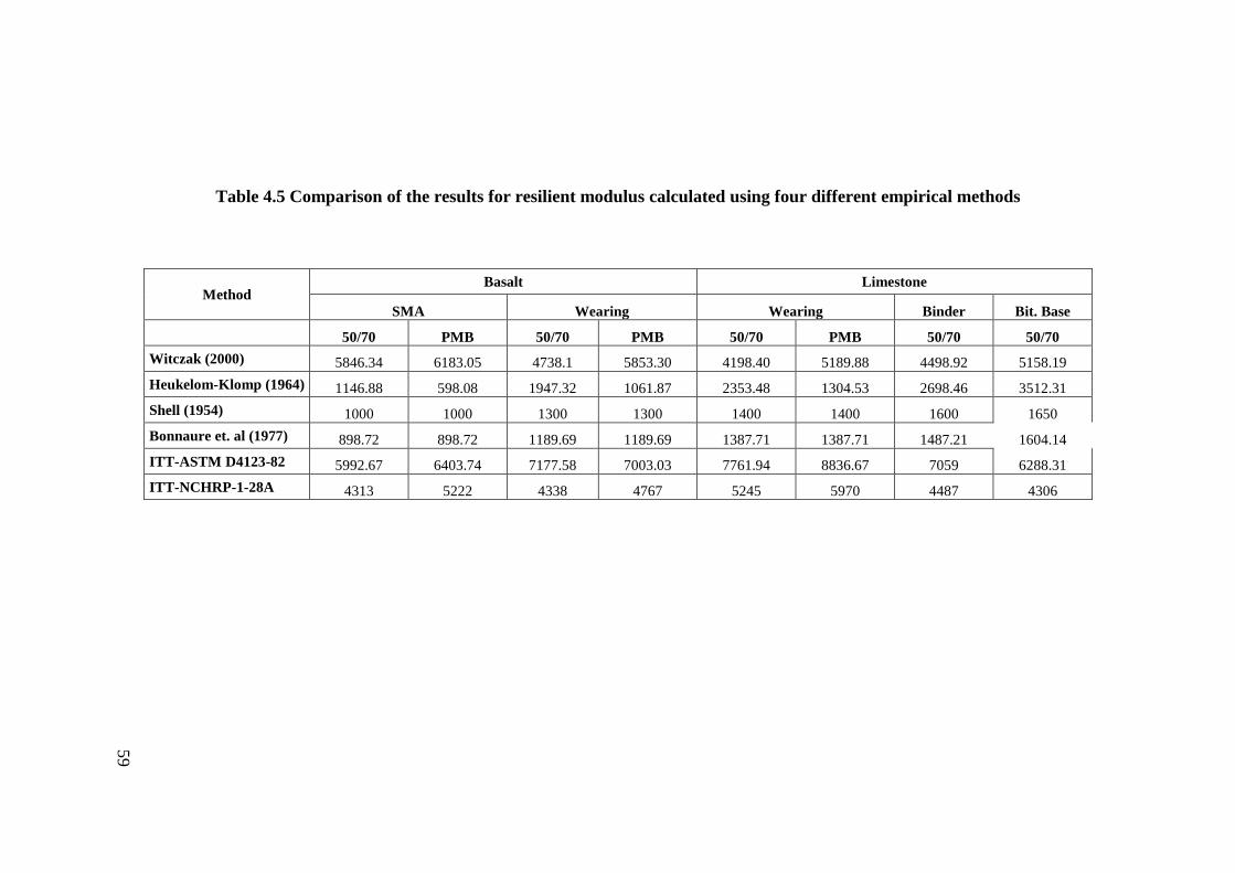
59
Table 4.5 Comparison of the results for resilient modulus calculated using four different empirical methods
Method Basalt Limestone
SMA Wearing Wearing Binder Bit. Base
50/70 PMB 50/70 PMB 50/70 PMB 50/70 50/70
Witczak (2000) 5846.34 6183.05 4738.1 5853.30 4198.40 5189.88 4498.92 5158.19
Heukelom-Klomp (1964) 1146.88 598.08 1947.32 1061.87 2353.48 1304.53 2698.46 3512.31
Shell (1954) 1000 1000 1300 1300 1400 1400 1600 1650
Bonnaure et. al (1977) 898.72 898.72 1189.69 1189.69 1387.71 1387.71 1487.21 1604.14
ITT-ASTM D4123-82 5992.67 6403.74 7177.58 7003.03 7761.94 8836.67 7059 6288.31
ITT-NCHRP-1-28A 4313 5222 4338 4767 5245 5970 4487 4306
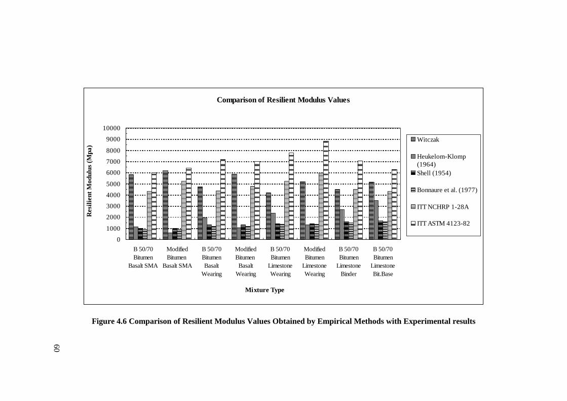
60
Comparison of Resilient Modulus Values
0
1000
2000
3000
4000
5000
6000
7000
8000
9000
10000
B 50/70
Bitumen
Basalt SMA
Modified
Bitumen
Basalt SMA
B 50/70
Bitumen
Basalt
Wearing
Modified
Bitumen
Basalt
Wearing
B 50/70
Bitumen
Limestone
Wearing
Modified
Bitumen
Limestone
Wearing
B 50/70
Bitumen
Limestone
Binder
B 50/70
Bitumen
Limestone
Bit.Base
Mixture Type
Resi
lien
t M
od
ulu
s (M
pa
)
Witczak
Heukelom-Klomp
(1964)
Shell (1954)
Bonnaure et al. (1977)
ITT NCHRP 1-28A
ITT ASTM 4123-82
Figure 4.6 Comparison of Resilient Modulus Values Obtained by Empirical Methods with Experimental results
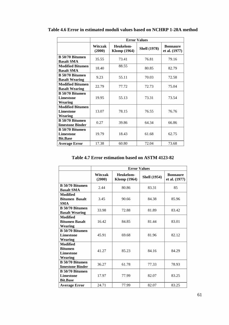
61
Table 4.6 Error in estimated moduli values based on NCHRP 1-28A method
Table 4.7 Error estimation based on ASTM 4123-82
Error Values
Witczak
(2000)
Heukelom-
Klomp (1964) Shell (1978)
Bonnaure
et al. (1977)
B 50/70 Bitumen
Basalt SMA 35.55 73.41 76.81 79.16
Modified Bitumen
Basalt SMA 18.40
88.55
80.85 82.79
B 50/70 Bitumen
Basalt Wearing 9.23 55.11 70.03 72.58
Modified Bitumen
Basalt Wearing 22.79 77.72 72.73 75.04
B 50/70 Bitumen
Limestone
Wearing
19.95 55.13 73.31 73.54
Modified Bitumen
Limestone
Wearing
13.07 78.15 76.55 76.76
B 50/70 Bitumen
limestone Binder 0.27 39.86 64.34 66.86
B 50/70 Bitumen
Limestone
Bit.Base
19.79 18.43 61.68 62.75
Average Error 17.38 60.80 72.04 73.68
Error Values
Witczak
(2000)
Heukelom-
Klomp (1964) Shell (1954)
Bonnaure
et al. (1977)
B 50/70 Bitumen
Basalt SMA 2.44 80.86 83.31 85
Modified
Bitumen Basalt
SMA
3.45 90.66 84.38 85.96
B 50/70 Bitumen
Basalt Wearing 33.98 72.88 81.89 83.42
Modified
Bitumen Basalt
Wearing
16.42 84.85 81.44 83.01
B 50/70 Bitumen
Limestone
Wearing
45.91 69.68 81.96 82.12
Modified
Bitumen
Limestone
Wearing
41.27 85.23 84.16 84.29
B 50/70 Bitumen
limestone Binder 36.27 61.78 77.33 78.93
B 50/70 Bitumen
Limestone
Bit.Base
17.97 77.99 82.07 83.25
Average Error 24.71 77.99 82.07 83.25

62
0
20
40
60
80
100
Witczak Heukelom-Klomp Shell Bonnaure et al.
Empirical Estimation Methods
Per
cen
t E
rror
ASTM D4123-82
NCHRP 1-28A
Figure 4.7 Percent error values for empirical methods used
63
CHAPTER 5
CONCLUSIONS
In this study, the resilient modulus values of different mixtures were determined by
experimental and empirical methods. For this study, 8 different types of mixtures
used in the design of asphalt concrete pavements in Turkey were prepared and then
subjected to indirect tension tests.
After experimental study, the resilient modulus values of the mixtures were
determined by various empirical methods suggested founding the literature, and the
results are evaluated in order to determine the best empirical method to estimate the
resilient modulus of tested mixtures. Based on the test results and the analysis of the
empirical methods, the following conclusions can be drawn:
- The ASTM method produces the highest modulus values as compared to the
NCHRP method. This outcome is attributed to the difference between the two
methods in terms of accuracy of the measured deformations and the calibrated
model coefficients used to calculate the resilient modulus.
- Heukelom-Klomp (1964), Bonnaure et al. (1977) and the Shell (1978) empirical
methods produce the lowest modulus values relative to the measured ones and
the Witczak (2000) predictive equation, hence they produce the largest estimation
errors.
- Witczak (2000) model produces the best approximation to the measured modulus
values with an average error of not more than 25%.
- It is recommended that in cases where the measured modulus value is not
available in the design phase of pavements, the Witczak (2000) predictive
equation be used to predict the actual modulus.
- Because the presented data in this study are quite limited, a larger data set should
be used to verify the presented results.

64
- Suggestions For Future Studies
In this study, resilient modulus of HMA mixtures consisting of wearing course, stone
mastic asphalt, binder and bituminous base courses are determined based on the
NCHRP test method. The results of this study should be supported by using a larger
data set to observe if the Witczak (2000) model always produces the best
approximation to the measured modulus. In addition, variability in the measured
resilient modulus due to non-uniform air void distribution of gyratory compactor
samples should be investigated by testing cut sections at different levels of
compacted samples.
65
REFERENCES
AASHTO (1993), Guide for Design of Pavement Structure, Washington, D.C.,
American Association of State Highway and Transportation officials, 1993.
ASTM Standard Test Designation D4123-82, Standard Test Method for Indirect
Tension Test for Resilient Modulus of Bituminous Mixtures, Annual Book of ASTM
Standards, ASTM, West Conshohocken, Philadelphia, U.S.A., 1995.
Atkins. H., Highway Materials, Soils, and Concretes, Prentice Hall; 4 edition, June
25, 2002.
Bonnaure F., Gest G., Gravois A., Uge P., A New Method of Predicting the Stiffness
of Asphalt Paving Mixtures. AAPT Proceedings, Volume 46, 1977, pp. 64-104
Brown E. R., Foo K. Y., Evaluatıon of Varıabıllly in Resilient Modulus Test Results
(ASTM D 4123-82. NCAT Report No. 91-6, 1989.
ÇÖLERĠ E., Relationship Between Resilient Modulus and Soil Index Properties of
Unbound Materials, M.S. Thesis, METU, 2007.
Gül. A.W., Effect of Recycled Cement Concrete Content On Rutting Behavior of
Asphalt Concrete, M.S. Thesis, METU, 2008.
Güngör A.G., Sağlık A., Karayolları Esnek Üstyapılar Projelendirme Rehberi,
Ankara, 2008
Güngör A. G., Orhan F., KaĢak S., Bitümlü Sıcak Karışım Aşınma Tabakalarının
Performanslarının İleri Deneyler İle Belirlenmesi, 5. Ulusal Asfalt Sempozyumu
Bildiriler, Ankara, 2009, pp. 277-288.

66
Güngör A. G., Sağlık A., Mekanistik Ampirik Üstyapı Tasarımında Esneklik
Modülünün ġartnamelere Uyarlanması, 5. Ulusal Asfalt Sempozyumu Bildiriler,
Ankara, 2009, pp. 289-298.
Güngör A. G., Sağlık A., Orhan F., Öztürk E. A., Polimer Modifiye Bitümlerin
Superpave Performans Sınıflarının Belirlenmesi, 5. Ulusal Asfalt Sempozyumu
Bildiriler, Ankara, 2009, pp 101-110.
Heukelom, W., Klomp, A. J., Road design and dynamic loading., Proceedings of the
Association of Asphalt Paving Technologists, Voume 33, pp.92-123
Huang. Y.H., Pavement Analysis and Design, Englewood Cliffs, New Jersey,
Prentice Hall, 1993.
Katicha W.S., Development of Laboratory to Field Shift Factors for Hot-Mix Asphalt
Resilient Modulus, M.S. Thesis, Faculty of the Virginia Polytechnic Institute and
State University, 2003.
Laboratory Determination of Resilient Modulus for Flexible Pavement Design: Final
Report, NCHRP Web Document 14, 1997.
National Cooperative Highway Research Program (NCHRP), Research Results
Digest, Number: 285, January 2004.
Necati K., Parameters which Affect the Stiffness of Bitumen and Bituminous Hot
Mixes, Turk J. Eng. Environ. Sci. 25 (2001) , pp 61 - 67.
Rahim A. M., Subgrade Soil Index Properties to Estimate Resilient Modulus for
Pavement Design, the International Journal of Pavement Engineering, Vol. 6, No. 3,
September 2005, 163–169.
Read J., Whiteoak D., The Bitumen Handbook
http://books.google.com.tr/books
67
Roberts F. L., Kandhal P S., Brown E.R., Lee D.Y., Kenedy T. W., Hot Mix Asphalt
Materials, Mixture Design and Construction, 2nd Edition,1996.
Seed, H.B., Chan, C.K., and Lee, C.E. “Resilience Characteristics of Subgrade Soils
and Their Relation to Fatigue Failures in Asphalt Pavements.” Proceedings of the
International Conference On the Structural Design of Asphalt Pavements, Ann
Arbor, Michigan: University of Michigan, 1962, pp. 611-636
Suhaibani A.Al., Sharaf E., Abdullatif A.Al., A Model ForAsphalt Concrete
Modulus Prediction From Basic Mix Variables In Saudi Arabaia, J. King Saud. Unv.
Vol 9, Eng. Sci. 1, pp 1-12.
Study of LTTP Laboratory Resilient Modulus Test Data and Response
Charecteristics, Final Report, Fugro-Bre Inc., 2001
Erkut S., and Harun T., Determine the Bituminous Hot Mixtures Stiffness with Fuzzy
Logic, Gazi Unv. Eng. Arc. Fac. Journal, Volume 21, No 4, 645-649, 2006.
Uluçaylı M., Türkiye' de Asfalt Betonu Kaplamalar ve Alternatifleri" Karayolları
Teknik Bülteni 16(65), Ankara, 1975
Ullidtz P., Pavement Analysis, Elsevier, Amsterdam.1987
UTS003 Indirect Tensile Test Software Reference, Ken de Vos, 2006
Van-der-Poel, C., A General System Describing the Visco-Elastic Properties of
Bitumens and Its Relation to Routine Test Data. J. Applied Chem., Volume 4, 1954,
pp. 221-236.
Yoder E. J., Witczak M. W., Principles of Pavement Design, pp. 269-275
http://books.google.com.tr/books

68
APPENDIX A
Indirect tension test set up parameters and test results.
Fig
ure
A.1
S
am
ple
Tes
t S
et u
p P
ara
met
ers

69
Fig
ure
A.2
S
am
ple
Tes
t R
esu
lts