EVALUATION OF NUMERICAL METHODS OF … · Thoma’s (1910) solution is used for surge tank design but ... numerical methods of solution for surge height analysis and compared with

International Research Journal of Engineering and Technology (IRJET) e-ISSN: 2395 -0056

Volume: 03 Issue: 11 | Nov -2016 www.irjet.net p-ISSN: 2395-0072

© 2016, IRJET | Impact Factor value: 4.45 | ISO 9001:2008 Certified Journal | Page 999

EVALUATION OF NUMERICAL METHODS OF SOLUTION AND RESISTANCE

EQUATIONS APPLICABLE TO UNSTEADY FLOW SITUATION IN SURGE TANK

Bharati Medhi Das1, Madan Mohan Das2, Bibhash Sarma3

1Assistant Professor, Civil Engineering Department, Assam Engineering College, Guwahati, Assam, India

2Formerly Professor of Civil Engineering Deptt, Assam Engineering College, Emeritus Fellow of AICTE, Director of Technical Education, Govt. of Assam, (Retd), India

3Associate Professor, Civil Engineering Department, Assam Engineering College, Guwahati, Assam, India ---------------------------------------------------------------------***---------------------------------------------------------------------

Abstract - In hydro-electric power plant, water is conveyed to the turbine through a long pipe. Sudden alteration of the flow rate can give rise to surges of pressure which move up and down the pipe causing knock. Closure of a valve at the downstream end of a pipe through which water is passing results in an immediate rise of pressure. To minimize the effect of pressure rise it necessitates the installation of a surge tank. This study aims to obtain a model solution for the given situation with numerical solution of the non-linear equation of continuity and momentum for a surge tank. Parallel investigations have also been made on how the transient friction factor of the pipe has played a dominant role to damp down the inertia pressure. The numerical solution is being assisted by resistance equations of Barr (1982), Romeo (2002), Fang (2011) and Brkic (2011). These are well applicable for all flow conditions ranging from laminar to turbulent. Comparison of the solutions is made with existing experimental data and also with data of another numerical solution done by Medhi Das and Sarma (2016) by Modified Jakobsen method. Both the numerical solutions have displayed quite a close agreement with experimental data. In the comparison, the numerical solution using resistance equations of Barr, Romeo and Fang shows a very good compromise with experimental data. But the solution with Brkic’s resistance equation is not tallying with the obtained laboratory values.

Key Words: knock, friction factor, model, unsteady, water

hammer.

1. INTRODUCTION : Sudden closure of valve during no load conditions gives rise to a very high inertia pressure within the pipe line. Kinetic energy of water is converted to elastic energy. Liquid is compressed and the pipe behaves as an elastic material, series of positive and negative waves travel back and forth until they are damped down by friction. The pressure rise may be so high that it may cause the pipe to burst if the prediction of pressure is not correct in the pipe. Therefore to minimize the effect of pressure rise it necessitates an adequate surge tank which reduces the amplitudes of water

hammer pressure and improves the governing characteristics of turbines. The stability of the oscillation of water level in the surge tank depends upon the type and size of the surge tank for given flow condition. Therefore, correct prediction of pressure rise is very important in the design consideration of the pipe and the surge tank and it depends largely on the selection of the resistance equation. Four suitable resistance equations based on logarithmic concept have been used in numerical solution with computer analysis. The method used in this study is the “Explicit finite difference method” to advance the solution of velocity and corresponding surge height in continuity and momentum equations.

2 REVIEW ON PREVIOUS WORKS :

Various hydraulic engineers have long been working to predict pressure rise in the surge tank. They have developed the various methods like graphical, analytical etc. The main fundamental equations of water hammer with or without a surge tank considering friction are non-linear. Classical solution cannot be used in practical application, as these solutions ignore the effect of friction. Graphical methods are approximate and do not give exact values. Thoma’s (1910) solution is used for surge tank design but cannot predict the maximum surge height. Pressel (1909) suggested a solution with constant turbulent friction factor. Jaegar’s (1954) solution gives only the values of maximum upsurge and down surge. Jakobsen (1969) used a finite difference method for complete closure of penstock valve. AIT, Bangkok (1969) presented a numerical solution similar to Jakobsen, which gave only the first maximum upsurge and first minimum down surge. Chattarjee (1965) developed direct step by step finite difference integration of the unsteady equations with the help of computer. He did not compare his solution with any model data. Elsden (1984) demonstrated a numerical approach in which maximum upsurge is been determined by different analytical and graphical methods. Barthakur (1997) presented numerical solution of unsteady equation where friction factor is calculated by Barr’s (1981) resistance equation and also performed a laboratory work. The results were then




compared and a good agreement was noticeable. They also compared with chatterjee’s solution but it did not display good agreement, it may be due to limitations of solution in respect of time step (5 sec) and use of constant friction factor value in Chatterjee’s solution. Das (1997) developed numerical methods of solution for surge height analysis and compared with laboratory data. Das et al. (2005) also worked on the numerical solution using Barr’s (1981) resistance equation. In this study the numerical method developed is the “Explicit finite difference method”. The solution so developed takes care of friction by using three recent resistance equations along with Barr’s resistance equation. Result so obtained are compared with the Modified Jacobsen method and existing experimental work. A review of the previously reported experimental data was undertaken. In Experimental work of Wood (1976), the length of pipe was only 36 feet with diameter 1.025 inches. His data presented were not of kind as required to assess numerical solutions. Simpson and Wylie (1991) also conducted experiments in a 36 m long pipe having 19.05 mm diameter. Pressure pulses are presented graphically for short durations, thus this type of data was not considered. Martin (1983) also conducted experiment work on the column separations situations. AIT, Bangkok (1969) has provided experimental data from an experimental setup of a large constant head reservoir with a 2 inch diameter pipe and 4.5 inch diameter clear plastic surge tank. The length of

the pipe was 28.76 feet and time interval was 1 to 28

seconds. Here, as the pipe length and time interval were very small, damping due to friction may not occur. Rao, P. V. et al. (1993) also studied on this work with laboratory set up. In this study laboratory data were taken from Das M. M. and Das Saikia M. (2016) for analysis. The experiment was conducted in Hydraulics laboratory of Assam Engineering College for time period up to 300 seconds.

3. BASIC EQUATIONS OF UNSTEADY FLOW IN SURGE TANK : Situations in a surge tank are illustrated in Figure 1 to Figure 4 along with the definitions of notations used in the equations.

Fig-1: Schematic illustrations before opening the penstock

valve in hydro-electric project

Fig–2: Schematic illustrations of steady state flow in hydro- electric project when turbines are taking load uniformly i.e. uniform discharge Q with steady velocity VO

Fig-3: Schematic illustrations of unsteady state (pressure rise in surge tank) in hydro-electric project when the valve is suddenly closed




Fig-4 : Schematic illustrations of unsteady state (pressure fall in surge tank) in hydro-electric project when the valve is suddenly closed

Where AS = area of the surge tank, At = area of the pressure

pipe, D= diameter of the pipe, f= friction factor, g =

acceleration due to gravity, hf= head loss due to friction,

L=length of the pipe line, Q = steady discharge in pressure

pipe, Qt = unsteady discharge in penstock, V0= steady velocity

in the pipe line before closing of the valve, V= unsteady

velocity in the pipe at any instant after valve closure, VS =

unsteady velocity in surge tank, Y= unsteady surge height at

any instant after valve closure.

Figure (1) shows the situation before opening the valve. Figure (2) shows the steady state condition of flow, when the uniform discharge Q flows with the steady velocity to the

power house. Figure (3) shows the unsteady flow situation at

any instant after the valve is partially closed. Water enters the surge tank initially with unsteady velocity Vs and the level of water in the surge tank goes on increasing due to water hammer pressure. It goes beyond the reservoir level and surge height becomes positive. After reaching a maximum height, it begins to fall again and surge height becomes negative as shown in Fig. (4). Thus surge height within the tank moves up and down with time and ultimately due to friction it damps down to zero level. In this unsteady situation, the velocity within the tunnel or pipe changes from steady state velocity Vo to unsteady velocity V. Due to partial closure of the valve, discharge also changes from Q to Qt. Now discharge from reservoir through the pipe after the valve closure is equal to At V. This discharge is equal to discharge enters the surge tank plus a discharge Q through penstock if valve is partially closed i.e.

( ASVS + Qt ).

Thus,

Continuity equation:

t

t

t

s

A

Q

dt

dy

A

Av

(1)

Momentum equation:

02

gD

VVfLy

dt

dV

g

L

(2) When the valve is completely closed, continuity equation becomes

dt

dy

A

Av

t

s

(3)

And substituting v from (3) in (2)

02

2

2

2

y

As

At

L

g

dt

dy

DAt

fAs

dt

yd

(4)

The resulting equation (4) is non-linear and it cannot be solved analytically.

4. EXPLICIT FINITE DIFFERENCE METHOD:

In this method, non-linear differential equations (1) and (2) are approximated by a pair of finite difference equations to advance the solution of velocity V and corresponding surge height y. The method is very simple and is very easy to handle by any field engineer. A very small time step ∆t is

taken. If j

kV and j

kY are the known velocity and surge

height at time j = 0 and at k position, at initial time (at the

steady state condition), values of 1j

kV and 1j

kY in the next

time step can be obtained by the following finite difference equations (7) and (8).

The finite difference forms of dt

dv and

dt

dy are:

t

VV

t

V j

k

j

k

1

(5)




t

yy

t

y j

k

j

k

1

(6)

Putting t

V

and

t

y

in the fundamental equation (1) and

(2) and simplifying,

The finite difference forms of (1) and (2) are

j

k

j

k

j

k

j

k

j

k VVgD

fLy

L

tgVV

2

1

(7)

j

k

s

tj

k

j

k VtA

Ayy .1

(8)

Then known values of 1j

kV and 1j

kY are initialized and

steps are repeated up to the desired time of solution.

5. RESISTANCE EQUATIONS:

The following resistance equations are used for friction factor calculation:

5.1 BARR’S EQUATION (1981)

The equation takes care of all state of flow conditions i.e. from laminar to turbulent.

89.010

1286.5

71.3log2

1

RD

k

f

(9)

5.2 ROMEO’S EQUATION (2002)

Valid for all ranges of Reynolds numbers and relative roughness

R

B

D

k

f

0272.5

7065.3log2

110

(10)

Where

9345.09924.0

10815.208

3326.5

7918.7log

RD

kA

R

A

D

kB

567.4

827.3log10

5.3 BRKIC’S EQUATION (2011)

Valid for all ranges of Reynolds numbers and relative roughness

2

4345.0

71.310log2

kf

(11)

Where

)1.11ln(

1.1ln816.1

ln

R

R

RS

5.4 FANG’S EQUATION (2011)

Fang developed an equation for friction factor based on R value ranges from 3000 to108 and (k/D) =0 to 0.05.

2

0712.11105.1

1007.1291.56525.60

234.0ln613.1

RRD

kf

(12)

Where D= diameter of pipe, f = friction factor, g = acceleration due to gravity, k = average sand roughness size, R = Reynolds number. For Reynolds number less than 1500, friction factor is calculated by using Poiseuille

equation, 25.0

3164.0

Rf .

6. COMPUTER INPUT DATA : Computer codes for MATLAB were written for explicit finite difference method to solve the two basic equations. The input data required for the computer program are: time

step head loss due to friction ( hf ), length of the pipe (L),

diameter of the pipe(D), steady discharge(Q), sand roughness

size (k), viscosity (VIS), Pi (PI), acceleration due to gravity (G)

and time of calculation (N).

Numerical input data are taken from experimental set up in the Hydraulics laboratory of Assam Engineering College. Initial values are taken from the steady state condition. Solutions are advanced up to 500 seconds after sudden closure of turbine valve with a very small time step of 0.5




seconds. Solutions for the variable surge height y and surge velocity V are obtained and are demonstrated by computer plot.

7. RESULTS AND DISCUSSIONS:

7.1 SURGE HEIGHT:

Figure 5 shows comparative plots of surge height with increasing time up to 500 seconds by Explicit finite difference method and experimental data when friction factor is assessed by all the resistance equations used and it is observed that solution with Barr, Fang and Romeo’s resistance equation, the results are well compromised, there is no significance difference between experimental and theoretical results. But with Brkic equation (Figure 5 and 6 ), initially it shows higher surge height and later it compromise with experimental result. It also shows that constant friction factor always gives maximum value of surge height. Figure 7 and 8 represents the comparison of the theoretical results obtained from Modified Jacobsen’s method and Explicit finite difference method with the experimental results by Romeo’s and Fang’s resistance equation respectively.

Fig-5 : Comparative plots of surge height vs. time by all

the resistance equations used with Explicit finite difference method and experimental result

Fig-6 : Surge height vs. time by Explicit finite difference method with Brkic’sresistance equation

Fig-7 : Comparative plots of surge height vs. time by Romeo’s resistance equation with Explicit finite difference method, Modified Jacobsen’s method and experimental data

Fig-8 : Comparative plots of surge height vs. time by Fang’s

resistance equation with Explicit finite difference method, Modified Jacobsen’s method and experimental data




In the computation of maximum surge height by implementing Barr, Romeo, Fang and Brkic’s resistance equation through explicit finite difference method and Modified Jakobsen’s method, it has been observed that the Explicit finite difference method has much more approximately closer value to the experimental model data than the value obtained from Modified Jakobsen’s method. Both the methods give almost same result. Furthermore among all the resistance equations implemented, Romeo’s resistance equation gives the most nearest value of maximum surge height to that of experimental model results and solution with Brkic resistance equation shows slightly higher value of surge height at the beginning. The results are exhibited in Table 1 for better comparison.

TABLE -1: COMPARISON OF RESULTS

Explicit Finite Difference method

Modified Jakobsen’s

method

Experimental model results

Res

ista

nce

eq

uat

ion

Max

. su

rge

hei

ght

(cm

)

Tim

e re

qd

. to

att

ain

max

. su

rge

hei

ght

(sec

)

Max

imu

m s

urg

e h

eigh

t (c

m)

Tim

e re

qd

. to

att

ain

max

. su

rge

hei

ght

(sec

)

Max

. su

rge

hei

ght

(cm

)

Tim

e re

qd

. to

att

ain

max

. su

rge

hei

ght

(sec

)

Barr 12.5 32.5 12.7 32

12

32.5

Romeo 12.2 33 12.5 33

Fang 12.4 32 12.6 32.5

Brkic 15.6 33 15.8 33

7.2 UNSTEADY VELOCITY: In Figure 9, 10, 11 and 12 velocity fluctuations with increasing time are shown. It is seen from these figures that before closing the valve, i.e. at time t=0, the magnitude of velocity is maximum that means the water is flowing through the pipe with its flow velocity. As soon as the valve is being closed, the magnitude of velocity decreases due to the obstruction in the path of flow. After closing of the valve, the fluctuation of velocity is noticed in the initial stage, but as the time goes on increasing the damping of velocity is

more pronounced and after some time it will attain a constant position i.e. the water comes to the rest.

Fig-9 : Velocity fluctuations by Explicit finite difference method with Brkic’s C-W friction factor

Fig-10 : Velocity fluctuations by Explicit finite difference

method with Romeo’s C-W friction factor

Fig-11: Velocity fluctuations by Explicit finite difference

method with Fang’s C-W friction factor




Fig-12 : Comparative plot of velocity vs. time by Explicit

finite difference method with all the resistance equations used

7.3 FRICTION FACTOR:

Variations of friction factor with time for the solutions are demonstrated in Figure 13, 14 and 15. These figures show how friction factor goes on increasing with time which proves that variable friction factor with time in every time step should be applied. Friction factor is calculated using Barr, Fang, Romeo and Brkic’s resistance equation at every time step as the solution proceeds. In all the cases some trends of increasing friction factor values with increasing time has been obtained. At the time when surge height is about to change its direction, friction factor values suddenly increase. Thus the increase in the friction factor also concludes that the flow condition changes from turbulent to laminar.

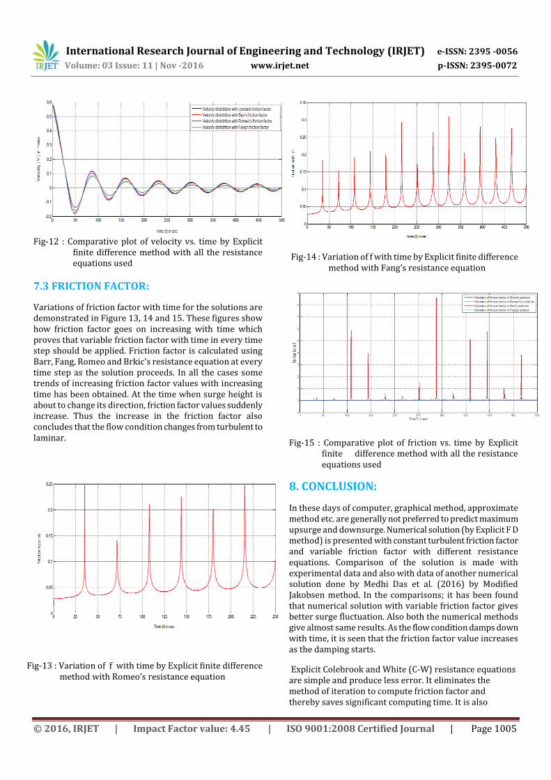
Fig-13 : Variation of f with time by Explicit finite difference method with Romeo’s resistance equation

Fig-14 : Variation of f with time by Explicit finite difference method with Fang’s resistance equation

Fig-15 : Comparative plot of friction vs. time by Explicit finite difference method with all the resistance equations used

8. CONCLUSION:

In these days of computer, graphical method, approximate method etc. are generally not preferred to predict maximum upsurge and downsurge. Numerical solution (by Explicit F D method) is presented with constant turbulent friction factor and variable friction factor with different resistance equations. Comparison of the solution is made with experimental data and also with data of another numerical solution done by Medhi Das et al. (2016) by Modified Jakobsen method. In the comparisons; it has been found that numerical solution with variable friction factor gives better surge fluctuation. Also both the numerical methods give almost same results. As the flow condition damps down with time, it is seen that the friction factor value increases as the damping starts.

Explicit Colebrook and White (C-W) resistance equations are simple and produce less error. It eliminates the method of iteration to compute friction factor and thereby saves significant computing time. It is also




observed by comparative study, among the various approximation of C-W, Romeo’s explicit approximation of C-W is somewhat better.

The principal parameters in the design of hydropower installations are surge tank diameter, height, the pipe or tunnel length and discharge. The computer model is so developed that keeping discharge Q, pipe length L, diameter D etc. are constant, maximum surge height (Ymax) after instantaneous valve closure can be predicted to fix the height of surge tank. Similarly when Q, L, Ymax etc. are known, diameter of the pipe can be predicted. Thus it can help to fix the required size or height of the surge tank or length of the pipe in the design purpose, when other parameters are fixed.

9. REFERENCES:

[1] Barr, D.I.H. (Dec, 1980) “Some Solution Procedures for C- W Function” Water Power and Dam Construction, London. [2]Barthakur, K. C. (1997) “Experimental and Theoretical

Studies of Water Hammer Pressure in Surge Tank and Pressure Conduit.”Ph D thesis submitted to Gauhati University.

[3]Chatterjee, P.N. (1995) Fluid Mechanics for Engineers,

Digital Computer Applications, 1st ed. MacMillan India Ltd.

[4]Colebrook, C.F. and white C.M. (1937) “Experiments

with fluid friction in Roughned Pipes” Proc., Royal Society of London, Series A, Vol. 161, pp. 367-381.

[5] Das, M, Sarma A.K. and Das M.M. (2005) “Effect of

resistance parameter in the numerical solutions on non linear unsteady equations in surge tank,” HIS Journal of Hy. Engg. Vol. II, No. 2, pp 101-110.

[6] Das. M.M. (1998) “Computer aided solution of surge

height and comparison with laboratory data”, presented and published in National Conference of Hydropower Dev. Central board of irrigation and water power(CBIP),New Delhi.

[7] Das, M.M.and Das Saikia M. (2016) “Irrigation and

water power Engineering”, a book published by PHI Learning),

[8] Elsden, O. (1984) “Hydroelectric Engineering Practice-

Surge Chambers” Editor- Brown, J. G., Vol. I, CBS Publishers and Distributors.

[9] Escande, L. (1950) “Methods Nonvelles pour le Cateul

des Chambers d’ equilibre” Dunod, Paris.

[10]Hydraulics Lab. Manual, (1969)Asian Institute of Technology, (AIT).

[11] Jaeger, C. (1956) “Engineering Fluid Mechanics”

Blakie and Sons Ltd., London. [12] Jakobsen, B. F. (1969) “Surge Tank” Trans. ASCE, 85,

PP 1357. [13] Medhi Das B. and Sarma B. (2016) “Solution of Non-

Linear Unsteady Flow Equation in Surge Tank” IJEERT, Vol.4 Issue 9

[14] Martin C.S. (1983) “Experimental investigations of Column Separation with Rapid closure of Downstream Valve” 4th Int.Conf. on “Pressure Surges” British Hy.Reseach Association, 77-88

[15] Pearsall, I. S. (1962): “A Survey of Surge Tank Design

Theories” NEL Report No.: 56. [16] Pickford, John (1969): “Analysis of Surges”

Machmilan,first edition. [17] Prasil, F.(1908) “Wasserschlossproleme” Schweij,

Banzig 52 [18] Pressel (1909, 1910, 1911) “Beitrag zur Bemesssung

des Inhaltes von Wasserschlossem” Scheweiz. Bauzlg. 53, 57 and 210.

[19] Rao P. V. et. al. (1993) “Validation of Reliability of

Transient Flow Analysis Program for Water Supply Systems”, Int. Conf. on Integrated Computer Applications for Water Supply and Distribution, De Mountford University, Leiveter, U. K. pp. 193-209.

[20] Saikia M. D. and Sarma A. K. (2006) “Numerical

Modelling of Water Hammer with Variable Friction Factor”, Proc. 2nd International Conf. of Comp. Mechanics and Simulations, IIT, Guwahati, 8-10 Dec.

[21] Simpson A. R. and Wylie E. B. (1991) “Large water

hammer pressures for column separation in pipelines”, ASCE Jour. Hy. Div. Vol. 117, Bangkok, A.I.T.

[22] Sulton, B.A. (1960) “Series Solution of Some Surge

Tank Prolems” Proc.Inst.Civil Engineers, Vol-16, pp225-234.

[23]Thoma, D. (1910):“Theorie des Wasserschlosses bei

Selbsttatiggeregelten Turbinenanlagen” Munchen,Verlag R, Oldenburg.

[24]Warren,M.M.(1915)“Penstock and Surge Tank ASCE.

Problems” Trans.




[25] Wood D.J. (1970) “Pressure Surge Attenuation Utilizing an Air Chamber”, ASCE Jour, Hy. Div. Vol. 96.

Documents

EVALUATION OF NUMERICAL METHODS OF … · Thoma’s (1910) solution is used for surge tank design but ... numerical methods of solution for surge height analysis and compared with