Evaluation of Neural Networks in the Subject of

International Journal of Engineering & Technology IJET-IJENS Vol:10 No:06 50

103706-5252 IJET-IJENS © December 2010 IJENS I J E N S

Abstract— Data driven prognostics employs many types of

algorithms some are statics and other are dynamics. Dynamic

complex engineering systems such as automobiles, aircraft, and

spacecraft require dynamic data modeling which is very efficient

to represent time series data. Dynamic models are complex and

increase computational demands. In previous work performed by

the author, linear regression model is provided to estimate the

remaining useful life left of an aircraft turbofan engines and

overcome the complexity of using dynamic models. It was simple

and efficient but it had some drawbacks and limitations. The

same task is resolved again here using multilayer perceptron

neural network (MLP NN). Results show that MLP NN as a static

network is extensively superior to linear regression model and

does not involve the complexity of dynamic models. Phm08

challenge data are used for algorithms training and testing. The

final score obtained from MLP NN can be placed in the fifteenth

position of the top 20 scores as published on the official site of the

Phm08.

Index Term— Multi Layer Perceptron NN, Prognostics,

Remaining Useful Life.

I. INTRODUCTION

Data driven prognostics is an efficient way to solve remaining

useful life (RUL) estimation of a dynamic complex

engineering systems such as automobiles, aircraft, and

spacecraft. The main advantage of using data driven

prognostics is to estimate RUL without any prior knowledge of

underlying physics of the system.

The operational and sensors data of dynamic systems are

always time series. Time series data represents operating

conditions and system parameters every time point. RUL

estimation of dynamic systems can be efficiently performed

using any dynamic modeling like recurrent neural network

used by Felix O. Heimes in [1]. Other time representation

methods are to use static modeling techniques with time

A.M. Riad is with Information System Department, Faculty of Computer

and Information Sciences, Mansoura University, Egypt.

Hamdy K. Elminir is with National Research Institute of Astronomy and

Geophysics, Department of Solar and Space Research, Egypt.

Hatem M. Elattar is with Information System Department, Faculty of

Computer and Information Sciences, Mansoura University, Egypt (email:

[email protected]).

delays. Both dynamic modeling and static modeling with time

delays increases network complexity and computational

demands. Leto Peel in [2] stated that "A significant

characteristic of the PHM Challenge dataset is that it contains

time series and therefore the representation of time or at least

how to represent and take account of previous temporal

observations is an important consideration. The quickest and

simplest method for representing time is to consider each time

point independently and create a prediction at each time step.

An alternative representation would be to consider using a

phase space embedding representation, in which a sequence of

instances is generated using a fixed length sliding window.

However phase space embedding has the significant drawback

of increasing the number of dimensions proportionally with

each time step represented, giving rise to the problems

associated with the 'curse of dimensionality'. From preliminary

experiments it was found that the prediction performance did

not improve significantly using the embedding space

representation given the increase in computational demands.

Therefore the chosen representation was to predict remaining

life using single time points".

The previous talk was the inspiration to use single time

point representation of time series data. A previous research

was performed named 'Forecast a remaining useful life of

aircraft turbofan engines based on a linear regression model'.

The previous work is in publication process, so a quick

summary will be given in a separate section below. The linear

regression model works fine but it has some drawbacks and

limitations which will be discussed latter.

Another approach is to use MLP NN as a static modeling

method and add indicators for the historical system run. This

approach used in [2] which describes the winning method in

the IEEE GOLD category of the PHM08 Data Challenge.

Work described in [2] adopts direct RUL estimation from data

based on all sensors readings and operating conditions. This

paper describes usage of MLP NN with back propagation

learning method to predict the system health of engines in test

data set for further RUL estimation. The health index of

engines in training data set is calculated based on the six

regression models obtained in the previous work done using

linear regression and work described in [3] and [4]. Only

Evaluation of Neural Networks in the Subject of

Prognostics As Compared To Linear Regression

Model

A. M. Riad, Hamdy K. Elminir, Hatem M. Elattar



thirteen sensors out of twenty one are utilized in MLP NN

training due to its behavior with degradation. Additional six

features which added to describe historical system run and the

three operating conditions are also included in training. The

same data preprocessing are applied to the test data set to

prepare the input to the network. The output values of HI for

engines in test data set are further smoothed and extrapolated

to calculate RUL for each engine. The developed algorithm

here is scored by the same score function described in [5]

which used to evaluate algorithms in 2008 PHM Data

Challenge Competition and gives a competitive score.

II. DATA OVERVIEW

The challenge data is obtained from prognostic-data-

repository of Prognostics Center of Excellence in National

Aeronautics and Space Administration (NASA) [6]. Data sets

are created by using high fidelity simulation system C-MAPSS

(Commercial Modular Aero- Propulsion System Simulation)

[7]. The process that describes how to use C-MAPSS to create

the proposed data is described in [5].

A data set consisting of multiple multivariate time series

is provided. This data set is further divided in to training and

testing subset. Each time series is from a different instance of

the same complex engineered system (referred to as a "unit")

the data here is about several aircraft engines of the same type

(turbofan engines). Each unit starts with different degrees of

initial wear and manufacturing variation which is unknown to

the user. This wear and variation is considered normal, i.e., it

is not considered a fault condition. There are three operational

settings that have a substantial effect on unit performance.

These settings are also included in the data. The data is

contaminated with sensor noise.

The unit is operating normally at the start of each time

series, and develops a fault at some point during the series. In

the training set, the fault grows in magnitude until system

failure. In the test set, the time series ends some time prior to

system failure. The objective is to predict the number of

remaining operational cycles before failure in the test set, i.e.,

the number of operational cycles after the last cycle that the

unit will continue to operate.

The training set includes operational data from 218 different

engines. In each data set, the engine was run for a variable

number of cycles until failure. The lengths of the runs varied,

with the minimum run length of 127 cycles and the maximum

length of 356 cycles. Fig. 1. shows two of the sensor

measurements from the first sequence in the training data. The

first sequence is 223 samples long. Fig. 1. (A) shows the first

two sensor readings as a function of time index and Fig. 1. (B)

shows the relationship between readings from the two sensors.

The lower plot shows that the readings are clustered around six

operating points and the variation around each operating point

is very small compared to the magnitude of the readings. The

upper plot shows that the readings jump from operating point

to operating point during each run.

. (A)

(B)

Fig. 1. Two of the sensor measurements from the first sequence in the

training data set. (A) First two sensors readings as a function of time

index.

(B) Readings are clustered around six operating points

There are three operational conditions that have a

substantial effect on unit performance (Altitude, Mach

number, and Throttle Resolver Angle). The operational

conditions for all engines can be clustered into six different

regimes as shown in Fig. 2. The six dots are actually six highly

concentrated clusters that contain thousands of sample points

each.

Fig. 2. Operational conditions of all engines are clustered into six

regimes.



III. SUMMARY ABOUT LINEAR REGRESSION MODEL

The previously created linear model was performed through

two main phases, learning and testing. In the learning phase

operating regime partitioning is performed to divide the

training dataset into six clusters each cluster represents single

operating regime. After rectangular regime partitioning sensor

readings for each regime are explored. Sensors can be

categorized into three groups as shown in Fig. 3. Sensors have

one or more discrete values, sensors have continuous values

but those values are inconsistent, and sensors have continuous

and consistent values.

(A)

(B)

(C)

Fig. 3. Different Sensor Groups. (A) Sensors have one or more discrete

values. (B) Sensors have continuous values but those values are

inconsistent. (C) Sensors have continuous and consistent values.

Health index is adjusted to value 1 for the first five cycles in

each engine run to indicate healthy engine, and to value 0 for

the time index exceeds 300 to indicate failed engine. For

models development only six sensors are selected from sensors

that have continuous and consistent values. Those six sensors

show high correlation with the health index. Six regression

models are built for the six regimes using linear least square

method in the form shown in (1).

N

i

ii xy1

(1)

Where x = (x1, x2, …, xN) is the N dimensional feature vector, y

is the health indicator, (α, β) = (α, β1, β2, …, βN) is N+1 model

parameters, and ε is the noise term.

After obtaining models parameter the testing phase is

started. Operating regime partitioning and sensors selection are

performed on the test data set. HI is calculated using the

obtained regression models for each regime. Data fusion of the

six clusters is performed to obtain a single data set which

contains HI for each engine run. For each engine HI is



smoothed using simple moving average then curve

extrapolated to calculate RUL for each engine run as shown in

Fig. 4.

RUL

tEOLti

Fig. 4. RUL Calculation

This algorithm is scored by the same score function

described in [5] which used to evaluate algorithms in 2008

PHM Data Challenge Competition and gives a score 6877.

Equation (2) shows the score function and Fig. 5. shows the

score as a function of the error.

(2)

Where s is the computed score, n is the number of UUTs

(Unit under test (Engine)), d = tˆRUL − tRUL (Estimated RUL –

True RUL), a1 = 13, and a2 = 10.

Fig. 5. Score as a function of error

The main drawbacks of using the previous method can be

summarized as follow:

1) The score is limited to 6877 as best obtained score which is

more than twice the score of the twentieth algorithm in the

top 20 scores list of algorithms on test data set.

2) Regression models could not be evaluated before applying

on test data set by methods like coefficient of

determination due to unavailability of HI data. This cause

requirement to check the efficiency of the model only on a

test dataset which is time consuming.

3) This model does not take into consideration previous time

points during its HI prediction.

4) Engines have few cycles of runs gives poor results in RUL

estimation.

Using of MLP NN can eliminate most of the previous

drawbacks and gives better results.

IV. METHODOLOGY

Multiple-layer networks are quite powerful. For instance, a

network of two layers, where the first layer is sigmoid and the

second layer is linear, can be trained to approximate any

function (with a finite number of discontinuities) arbitrarily

well. This kind of two-layer network is used extensively in

back propagation. Two layers MLP NN with twenty two

inputs, twenty nodes in hidden layers, and single node output

layer is trained by back propagation to predict engine health

index for further curve smoothing and extrapolation to

estimate RUL. Number of nodes in hidden layers is chosen by

trial and error. Rough approximation can be obtained by the

geometric pyramid rule. According to this rule, for the three

layer network (considering input layer as third layer) with n

input and m output. The number of neurons in hidden layer

was adjusted according the previous rule, then increasing the

number of nodes to achieve best fit. Regarding not to increase

number of nodes in hidden layer to a large number is taken

into consideration to avoid over fitting. Activation function

used in hidden layer is tan-sigmoid transfer function and in the

output layer is linear transfer function. The work here can be

divided into three main stages; Data preparation, Training, and

Testing (simulation).

A. Stage 1: Data Preparation

1) Sensors Selection: From data analysis as shown in Fig. 3.

sensors categorized in to three different groups. Here sensors

have continuous and consistent values which determine a

degradation trend of engines are chosen (9 sensors). In

addition sensors have continuous values but those values are

inconsistent also chosen (4 sensors). Although those sensors

have not been used in regression models creation it will be

used as input to the network. Those sensors can give additional

knowledge to the network like difference between modes or

other hidden information that the network could discover

implicitly. Only sensors that have one or more discrete values

are not chosen due to their irrelevance (7 sensors). Total



number of sensors used to train the network is thirteen sensors

to enhance network behavior as suggested in the future work in

[2] and [4]. As long as it is well known that from [5] the

operational settings have a substantial effect on unit

performance, it will be used as an input to train the network.

2) Normalization: Data normalization is performed to give a

uniform scale in a data set. The following formula in (3) is

used for data normalization.

dx

xNd

ddd

,)(

(3)

Where xd are the original data values for feature d, and d, d

are the mean and standard deviation respectively for that

feature. Further normalization is performed in each mode to

maximize the variance between modes as in [2]. Formula in

(4) describes this normalization process.

dmx

xNdm

dmdmdm ,,)(

),(

),(),(),(

(4)

Where m refers to one of the six possible modes (regimes).

3) Sensors Reading Smoothing: The sensors data is

contaminated with noise. Simple moving average is used to

smooth sensors measurements for each engine in each regime.

Fig. 6. shows the normalized and smoothed data of S2

measurements for engine number one in the first regime.

Fig. 6. Normalized and smoothed data of S2 measurements for engine number

one in the first regime.

4) Adding Historical Run Indicator: Additional six features

are added to represent total number of cycles spent in mode

since the beginning of run. Those extra six features give a

good indication of historical run in each mode to enhance the

usage of static network. Fig. 7. shows the number of cycles

spent in each mode for the first engine in sequence.

Fig. 7. Number of cycles spent in each mode for the first engine in

sequence.

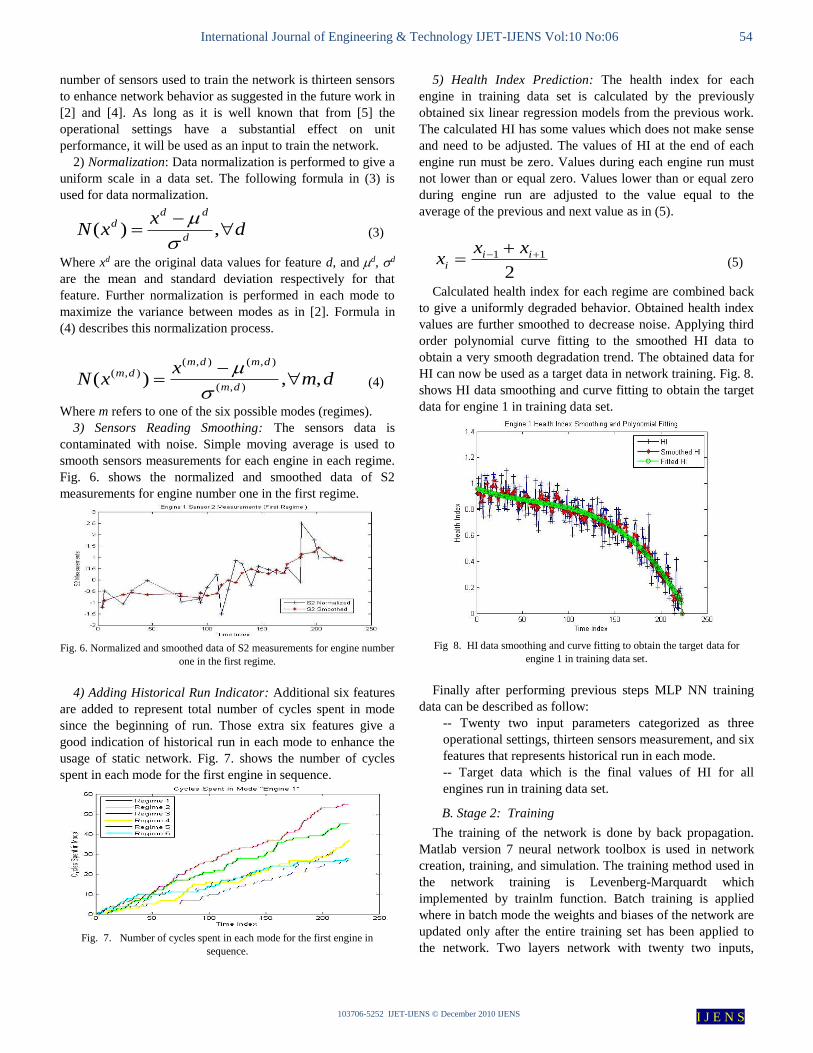
5) Health Index Prediction: The health index for each

engine in training data set is calculated by the previously

obtained six linear regression models from the previous work.

The calculated HI has some values which does not make sense

and need to be adjusted. The values of HI at the end of each

engine run must be zero. Values during each engine run must

not lower than or equal zero. Values lower than or equal zero

during engine run are adjusted to the value equal to the

average of the previous and next value as in (5).

2

11 ii

i

xxx (5)

Calculated health index for each regime are combined back

to give a uniformly degraded behavior. Obtained health index

values are further smoothed to decrease noise. Applying third

order polynomial curve fitting to the smoothed HI data to

obtain a very smooth degradation trend. The obtained data for

HI can now be used as a target data in network training. Fig. 8.

shows HI data smoothing and curve fitting to obtain the target

data for engine 1 in training data set.

Fig 8. HI data smoothing and curve fitting to obtain the target data for

engine 1 in training data set.

Finally after performing previous steps MLP NN training

data can be described as follow:

-- Twenty two input parameters categorized as three

operational settings, thirteen sensors measurement, and six

features that represents historical run in each mode.

-- Target data which is the final values of HI for all

engines run in training data set.

B. Stage 2: Training

The training of the network is done by back propagation.

Matlab version 7 neural network toolbox is used in network

creation, training, and simulation. The training method used in

the network training is Levenberg-Marquardt which

implemented by trainlm function. Batch training is applied

where in batch mode the weights and biases of the network are

updated only after the entire training set has been applied to

the network. Two layers network with twenty two inputs,



twenty nodes in hidden layer with tan-sigmoid transfer

function, and single node output layer with linear-transfer

function gives R = 0.98783 and MSE = 0.00171 Where R and

MSE are the correlation coefficient and mean squared error

between network output and target data respectively. The

previous output obtained from single stage training. The

results seem great so there is no need for additional training.

B. Stage 3: Testing (Simulation)

1) The first four steps in data preparation stage (Sensors

selection, Normalization, Sensors reading smoothing, and

Adding Historical Run Indicator) are applied to test dataset.

2) The trained network is simulated to predict health index

for engines in test data set.

3) Health index calculated to each engine is further

smoothed using simple moving average.

4) Second and third order polynomial curve fitting is

applied on the smoothed health index data.

5) Extrapolation of polynomial curve is done until the health

index value reaches zero.

6) RUL is calculated by subtracting the time at the point of

prediction (ti) from the time at engine end of life (tEOL) (Fig.

9).

RUL = tEOL - ti (5)

Fig. 9. RUL Calculation

V. RESULTS AND DISCUSSION

The developed algorithm gives early prediction for 195

engines, late prediction for 8 engines, and exact prediction for

15 engines. The overall score of the algorithm based on the

score function in (2) is 1540 which can be placed between the

fourteenth and fifteenth score of the top 20 scores as published

on the official site of the Phm08 (Fig. 10).

Fig. 10. Top 20 scores list of algorithms on test data set

Results show that MLP NN is working better linear

regression model in solving this type of problems. MLP NN

gives more smoothed values of HI which leads to better

prediction. Also MLP NN show better behavior with engines

has few cycles of run. The following table shows the

difference in performance between MLP NN and linear

regression model.

TABLE 1

MLP NN PERFORMANCE VS. LINEAR REGRESSION MODEL

MLP NN Linear

Regression

Model

Score 1540 6877

Early Prediction 195 131

Late Prediction 8 63

Exact Prediction 15 24

Mean Square Error Between

Estimated RUL and Actual RUL 345.46 390.44

Correlation Coefficient Between

Estimated RUL and Actual RUL 0.9414 0.88

RUL forecast depends on the

current and previous cycles during

engine run

Yes No

Forecasting in case of few cycles of

engine run Good Poor

Smoothness of predicted health

index data Very Good Acceptable



VI. CONCLUSION

In this paper MLP NN with back propagation learning as a

static network proofs its ability to solve a problem of RUL

estimation of a dynamic complex engineering system (aircraft

turbofan engine). This method involves prediction of HI first

to use it in RUL estimation. Additional work is done to

improve features (sensors) selection as recommended in future

work in [2] and [4]. Comparison between performance of MLP

NN and linear regression model is done which proofs

superiority of MLP NN over linear regression model in solving

complex forecasting tasks.

REFERENCES [1] Felix O. Heimes, BAE Systems "Recurrent Neural Networks for

Remaining Useful Life Estimation" 2008 international conference on

prognostics and health management.

[2] Leto Peel, Member, IEEE (GOLD) " Data Driven Prognostics using a

Kalman Filter Ensemble of Neural Network Models" 2008

international conference on prognostics and health management.

[3] T. Wang, and J. Lee, “The operating regime approach for precision

health prognosis,” Failure Prevention for System Availability, 62th

meeting of the MFPT society - 2008, pp. 87-98.

[4] Tianyi Wang, Jianbo Yu, David Siegel, and Jay Lee "A Similarity-

Based Prognostics Approach for Remaining Useful Life Estimation of

Engineered Systems" 2008. International conference on prognostics

and health management.

[5] Abhinav Saxena, Member IEEE, Kai Goebel, Don Simon, Member,

IEEE, Neil Eklund, Member IEEE "Damage Propagation Modeling for

Aircraft Engine Run-to-Failure Simulation" May 18, 2008.

[6] http://ti.arc.nasa.gov/tech/dash/pcoe/prognostic-data-repository/

[7] D. Frederick, J. DeCastro, and J. Litt, "User’s Guide for the

Commercial Modular Aero-Propulsion System Simulation

(CMAPSS)," NASA/ARL, Technical Manual TM2007-215026, 2007.

[8] Girish Kumar JHA "Artificial Neural Network" Indian Agricultural

Research Institute, PUSA, New Delhi 110012.

[9] M. Tim Jones "Al Application Programming" Charles River Media ©

2003.

[10] NASA Ames Research Center "Integrated System Health Management

(ISHM) Technology Demonstration Project Final Report" December

15, 2005.

[11] Mark Schwabacher and Kai Goebel "A Survey of Artificial

Intelligence for Prognostics" NASA Ames Research Center,2008.

[12] Ian H. Witten, Eibe Frank, Department of Computer Science

University of Waikato "Data Mining Practical Machine Learning Tools

and Techniques, Second Edition", 2005.

[13] Kai Goebel, Bhaskar Saha, Abhinav Saxena, NASA Ames Research

Center "A comparison of three data-driven techniques for prognostics",

2008.

http://ti.arc.nasa.gov/tech/dash/pcoe/prognostic-data-repository/

Documents

Evaluation of Neural Networks in the Subject of