Evaluation of Natural Language Processing Techniques for Sentiment Analysis on Tweets

Bachelor Thesis von Dang, Thanh Tung

October 2012

Betreuer: Prof. Dr. Johannes Fürnkranz

Verantwortliche Mitarbeiter: Dr. Heiko Paulheim (TU Darmstadt)

Dipl.-Wirt. Inform. Axel Schulz (SAP Research)

Vorgelegte Bachelor-Thesis von Dang, Thanh Tung

1. Gutachten:

2. Gutachten:

Tag der Einreichung:

Erklärung zur Bachelor-Thesis

Hiermit versichere ich, die vorliegende Bachelor-Thesis ohne Hilfe Dritter nur mit den angegebenen Quellen und Hilfmitteln angefertigt zu haben. Alle Stellen, die aus Quellen entnommen wurden sind

als solche kenntlich gemacht. Diese Arbeit hat in gleicher oder ähnlicher Form noch keiner

Prüfungsbehörde vorgelegen.

Darmstadt, den 15. Oktober 2012

________________________________________ (Dang, Thanh Tung)

Contents

Contents iii

1. ..... Introduction 1

1.1. Motivation 1

1.2. Problem description 1

1.3. Goal of the Thesis 1

1.4. Structure of the Thesis 2

2. ..... Basic 3

2.1. Micro-blog 3

2.2. General emotions of human being 3

2.3. Machine learning 3

2.3.1. Naïve Bayes 4

2.3.2. Support Vector Machine 5

2.3.3. Terminologies in machine learning 6

2.4. Opinion mining/Sentiment analysis/ Subjectivity analysis 6

3. ..... Sentiment Analysis on Text 8

3.1. Problem and methods for Sentiment Analysis 8

3.1.1. Sentiment Analysis at document level 8

3.1.2. Sentiment Analysis at sentence level 9

3.1.3. Sentiment Analysis at word/phrase level 9

3.2. Resources and tools for Sentiment Analysis on Tweets 10

3.2.1. Abbreviation and slang 10

3.2.2. AFINN word list (Nielsen, 2011) 10

3.2.3. Emoticons 10

3.2.4. Part of speech tagger (POS-tagger) 11

3.2.5. Wordnet 12

3.2.6. SentiWordnet 12

3.2.7. DKPro 13

3.2.8. Weka 13

3.3. State of the art 14

4. ..... Experiment setup 18

4.1. Data sets 18

4.2. Evaluation methods 21

5. ..... Evaluation methods for English data sets 22

5.1. Structure of evaluation methods for English data sets 22

5.2. Tweet preprocessing 22

5.3. Feature engineering 23

5.3.1. Word unigram extraction 24

5.3.2. Word unigram extraction + Concept replacement 24

5.3.3. Word unigram extraction + POS tagging 24

5.3.4. Character tri-gram extraction 25

5.3.5. Character four-gram extraction 25

5.3.6. Syntactic features extraction 25

5.3.7. Sentiment features extraction 26

5.4. A simple classifier for 3-ways classification task 27

6. ..... Evaluation methods for the Vietnamese data set 30

7. ..... Evaluation results 31

7.1. Evaluation results on the English data sets 31

7.1.1. Using only word unigram 31

7.1.2. Using word unigram after replacing named entities with concepts 32

7.1.3. Using word unigram with POS-tagging 33

7.1.4. Using only syntactic and sentiment features 33

7.1.5. Using character tri-gram 34

7.1.6. Using character four-gram 34

7.1.7. Results of the simple classifier 36

7.2. Evaluation result on the Vietnamese data set 37

8. ..... Conclusion 38

8.1. Summary 38

8.2. Outlook and future works 38

List of tables 1

List of figures 1

9. ..... Bibliography 2

1

1. Introduction

1.1. Motivation

For crisis management, information is a crucial resource to assist coordinators in understanding the

current situation. Considering as much information as possible helps them to identify the appropriate

set of perception elements as well as utilize the comprehension patterns/templates of higher level and

forecast operators (Cameron, Power, Robinson, & Yin, 2012). With increasing use of Twitter as a

communication channel, the analysis of tweet messages could not only bring about multidimensional

understanding but also contribute to decision making in crisis management. For example, sentiment analysis from tweet messages during an event which negatively affects massive audience could help to

detect and to track an ongoing panic. Also, the sentiment analysis facilitates the personnel in charge

(e.g. police, ambulance) to make decisions to prevent possible consequences. The challenge is that,

sentiment analysis on tweets has not been popular in crisis management, because tweet messages are

mostly not authoritative and contain irrelevant information (Cameron, Power, Robinson, & Yin, 2012).

Much attention in the crisis management focused only on the information sources around the

situation. Therefore, our vision is such that the utilization of sentiment analysis during disasters could

improve the situational awareness by providing proactive information about the scenario.

To our awareness, there has been certain work about sentiment analysis on text such as the work of Bo

Pang and Lillian Lee (Pang & Lee, Opinion Mining and Sentiment Analysis, 2006). However, a specific methodology for tweets is still on demand when designing the crisis management system, which uses

tweet messages as one of information sources.

1.2. Problem description

In this work, the primary question for sentiment analysis is how to map a tweet to a correct emotion,

which user tried to express. The first problem is unstructured, ungrammatical text. Since tweet

messages are restricted to 140 characters length, users may have a propensity to use abbreviations, slangs, or emoticons to shorten the text. This issue can lead to unusual messages.

The second problem is the fact that tweet messages are not always correct. During fast typing, or using

mobile phones as input device, user may have mistyped text and make the analysis step harder.

The third problem is ambiguity. Due to the small amount of information, it is difficult to identify the

corresponding objects of interest. For example: “Apple” can either be a laptop brand or a fruit.

The fourth problem concerns which concrete emotion to focus on analyzing since human emotion is

very diverse.

1.3. Goal of the Thesis In this thesis, we will focus on evaluation of some widely used natural language processing techniques,

machine learning methods and tools for sentiment analysis. We compare how well they perform on

tweet messages and therefore propose the suitable methods for dealing with some information

channels, in which only small amount of texts are available. It will benefit other researchers by

reducing time for choosing tools and methods.

2

1.4. Structure of the Thesis

This remaining of this thesis will be structured as follows:

Chapter 2 introduces some background knowledge:

An introduction of micro-blogs, especially about Twitter

An overview of general human emotions and which aspects are necessary to distinguish them

Some basic definitions and algorithms in machine learning field are described

The work of sentiment analysis and its goals are introduced in this part

The third chapter describes the problems and methods for analyzing sentiment on text and on tweets

respectively. The resources and tools for the process will be explained here. At the end of this chapter,

a summarization of state-of-the-arts gives us an overview of the approaches and their performances.

In chapter 4, we describe the data collecting procedure, in which four data sets are used. Those data

sets contain tweet messages in two different languages i.e. English and Vietnamese. The detail about

those data sets will be illustrated.

The different approaches for analyzing sentiment in the English data sets are explained in the fifth

chapter.

The sixth chapter concerns itself with the different approaches for the Vietnamese data set.

In the seventh chapter, the result and performance of each approach are discussed. Methods and tools are compared in this chapter.

Finally, we conclude this thesis with an overview of the results as well as propose several suitable

methods and future extensions for analyzing sentiment on tweet messages.

3

2. Basic

In this section, we introduce some basic definitions that are related to our work: the definition of

micro-blog and Twitter, the general emotions of human being, some basic definitions in machine

learning field and an overview of sentiment analysis on text.

2.1. Micro-blog

Micro-blog is a term which indicates the short text created by user using online services like Twitter1,

Facebook2, and Tumblr3 in order to provide updates on their activities, observations and interesting content (Ehrlich & S., 2010). This term is also used to refer to those online services.

This paper concerns itself only with Twitter, which is created by Jack Dorsey in March 20064. In

Twitter, users are allowed to post message, which is called tweet, within 140 characters long5. In order

to convey information with this restriction, users use several conventions as listed below:

Hashtag(#) followed by one word or code to group the related messages. For example: #euro2012

A @ sign followed by a username to mention that the post is directed to this user. For example:

@BarackObama

Re-tweet: means that the user quotes the message of another people by copying their post and

username.

2.2. General emotions of human being

According to Ekman (Ekman, 1992), the main function of emotion is to mobilize the organisms to deal

quickly with the encounters, between people; or between people and other things or facts. Each

individual emotion is not a single state but contains multiple related states: not only facial expression

but also speech, or writing. The combination of those states will lead to different emotion expressions

and people thus can have a number of discrete emotions. However, they share some common

characteristics and can be grouped into some basic families. Ekman proposed six basic human emotion’s families: anger, disgust, fear, happiness, sadness, surprise and also nine characteristics which

distinguish those basic emotions (Ekman, 1992).

At the moment, the techniques for measuring human expression are mostly based on the analysis of

the muscular expressions. In other words, the strongest evidences for distinguishing one emotion from

another are facial states. However, in this paper we will focus on analyzing human emotions only

relying on their writing.

2.3. Machine learning

According to English Oxford Dictionary6, the verb “to learn” is described as:

“Gain or acquire knowledge of or skill in (something) by study, experience, or being taught

To commit to memory

To become aware of something by information or from observation”

However, this definition of the verb “to learn” is virtually impossible to test with machines (Witten &

Frank, 2005). In other words, learning implies thinking and purpose; with computer, they are

1 http://www.twitter.com/

2 http://www.facebook.com/

3 http://tumblr.com/

4 http://en.wikipedia.org/wiki/Twitter

5 http://twitter.com/about

6 http://oxforddictionaries.com/definition/learn?q=learn

4

nontrivial. Thus, Witten and Frank preferred using the word “training” to denote a mindless kind of

learning (Witten & Frank, 2005).

We only use a simple aspect of their interpretation for machine learning: computer is trained with inputs and accomplishes the tasks we give. There are many different tasks in machine learning such as

text classification, regression problem7 or sequence labeling8 but the main problem considered in this

thesis is text classification: Given a set of documents and a set of classes: . Some documents are already assigned with a label, which denotes the class the documents belong to.

Our task is to assign each unlabeled document with one correspondent class.

Three used algorithms for solving this problem are described as below.

2.3.1. Naïve Bayes

Naïve Bayes Classifier is a simple probabilistic classifier based on applying Bayes’ theorem with strong

(naïve) independence assumption that: the presence of one feature in a class does not depend on the

presence or absence of another feature.

The features or also known as attributes are the characterized values to describe an instance (in this

case a document). Each individual instance is defined by its value on a fixed, predefined set of features

or attributes (Witten & Frank, 2005). For example, in the text classification problem, the features can be extracted from words in a document.

The independence assumption does not hold in real texts because of the grammatical relation between

words in the sentence. For example: a sentence is meaningless if it contains only verbs and adjectives.

However, it turns out that it can still be used in practice, especially in this case of tweet messages when

they are mostly ungrammatical.

We assume that each document is now represented as a vector: | | where is the word

in position and | | is the number of words in this document. The probability that a document d

belong to class c is: | . The classification problem is now solved by calculating the probabilities:

| for each class and choosing the class with the greatest probability. According to Bayes

Theorem, the probability that the document d belongs to class c is calculated as below:

| |

| |

Where:

| is the probability that all words in the document d appear in class c together

is the prior probability of class c (the distribution of classes) determined by the fraction of

documents that are of class c.

is the prior probability of the document d and it can be omitted because we only have to compare | in order to choose the best class.

We have:

| (( | |)| ∏ |

| |

7 http://en.wikipedia.org/wiki/Regression_analysis

8 http://en.wikipedia.org/wiki/Sequence_labeling

5

In which:

| ∑

∑ | |

is the probability that the word occurs in class c.

It is calculated by the number of time that the word appear in all the documents d, which belong to

class C divided by the total number of word in documents in this class.

It should be noted that when a document contains new word, which does not appear in the labeled documents, it will assign probability 0 for all classes because of:

|

To deal with this problem we use Laplace correction: assuming that each word occurs in a document at

least one time to calculate | :

| ∑

| | ∑ | |

Where | | is the number of distinct words in all documents. Obviously, the formulas are only

applicable under the independence assumption.

With this algorithm, we consider two representations of a document:

Naïve Bayes Binary Model (NBB): only presence or absence of words are considered

Naïve Bayes Multinomial Model (NBM): multiple occurrence of words are considered

For instance, the sentence “my mother is a teacher and my father is a doctor” is represented as vector

of words in two models as below:

NBB: (my, mother, is, a, teacher, and, father, doctor)

NBM: (my, mother, is, a, teacher, and, my, father, is, a, doctor)

2.3.2. Support Vector Machine

Another algorithm for solving the text classification problem is Support Vector Machine (SVM)

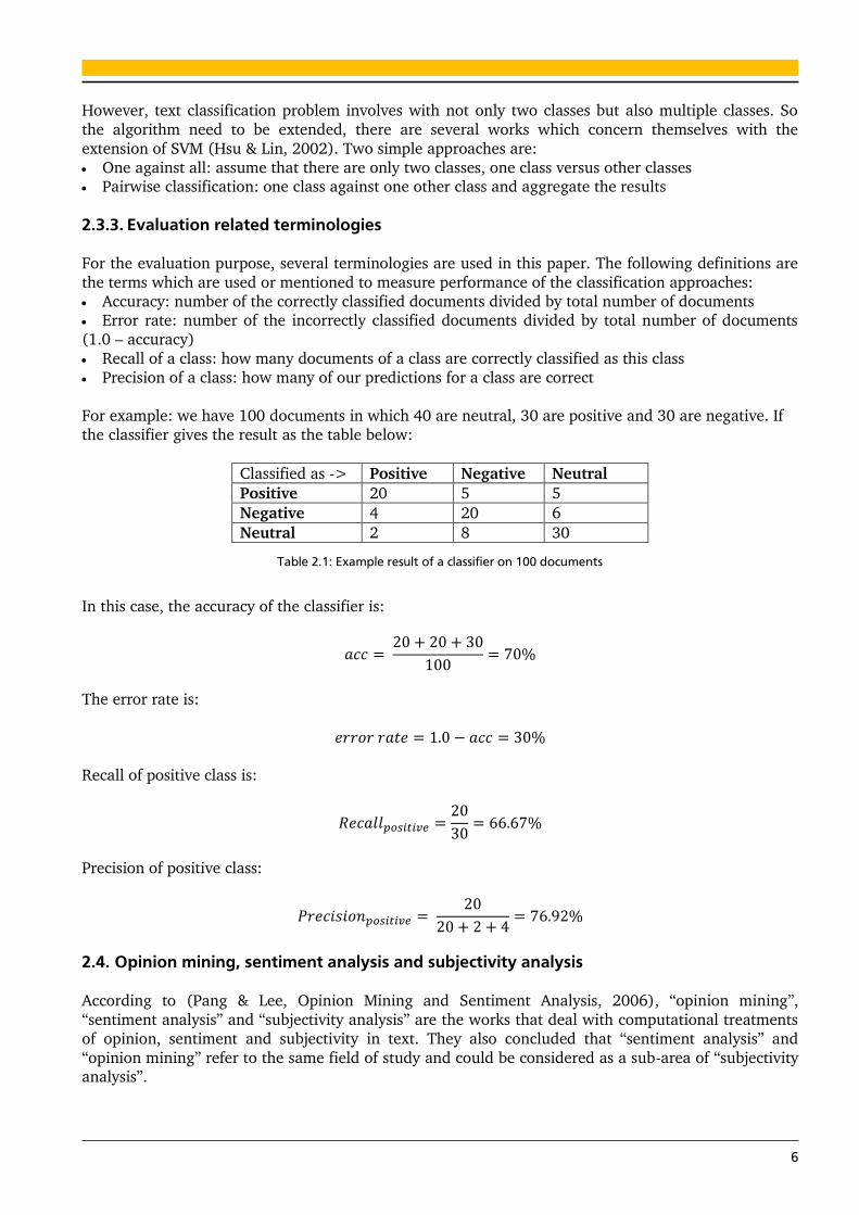
introduced by (Cortes & Vapnik, 1995). The idea of this algorithm is to consider each document as a

point in the document space and to find the appropriate hyperplane to separate the documents into

two classes. The following picture depicts a sample view of the algorithm:

Figure 2.1: Documents belong to two classes and the hyper plane which separates them. (Cortes & Vapnik, 1995)

6

However, text classification problem involves with not only two classes but also multiple classes. So

the algorithm need to be extended, there are several works which concern themselves with the

extension of SVM (Hsu & Lin, 2002). Two simple approaches are:

One against all: assume that there are only two classes, one class versus other classes Pairwise classification: one class against one other class and aggregate the results

2.3.3. Evaluation related terminologies

For the evaluation purpose, several terminologies are used in this paper. The following definitions are

the terms which are used or mentioned to measure performance of the classification approaches:

Accuracy: number of the correctly classified documents divided by total number of documents Error rate: number of the incorrectly classified documents divided by total number of documents

(1.0 – accuracy)

Recall of a class: how many documents of a class are correctly classified as this class

Precision of a class: how many of our predictions for a class are correct

For example: we have 100 documents in which 40 are neutral, 30 are positive and 30 are negative. If

the classifier gives the result as the table below:

Classified as -> Positive Negative Neutral

Positive 20 5 5

Negative 4 20 6

Neutral 2 8 30

Table 2.1: Example result of a classifier on 100 documents

In this case, the accuracy of the classifier is:

The error rate is:

Recall of positive class is:

Precision of positive class:

2.4. Opinion mining, sentiment analysis and subjectivity analysis

According to (Pang & Lee, Opinion Mining and Sentiment Analysis, 2006), “opinion mining”,

“sentiment analysis” and “subjectivity analysis” are the works that deal with computational treatments

of opinion, sentiment and subjectivity in text. They also concluded that “sentiment analysis” and

“opinion mining” refer to the same field of study and could be considered as a sub-area of “subjectivity analysis”.

7

The analysis process may have different goals but they could be boiled down to opinion-related

information extraction. Like many other information extraction tasks, sentiment analysis could be

performed at several levels of context. Three basic of them are:

Document level Sentence level

Term/phrase level

The basic problems and methods to deal with those problems at each level will be discussed in the next

section.

8

3. Sentiment Analysis on Text

In this chapter, the details about sentiment analysis on text are described in three parts. The first part

concludes the problems and general methods for sentiment analysis at different levels. In the second

part we introduce tools and programming frameworks for text processing as well as machine learning.

And the last part summarizes state-of-the-art in sentiment analysis on tweets.

3.1. Problem and methods for Sentiment Analysis

The three following sections will discuss about the main problem and some related approaches at each level.

3.1.1. Sentiment Analysis at document level

The basic problems of Sentiment Analysis comprise the analysis of opinions in a document. There are

several scales for the classification of opinion but according to (Jakob, 2011) the most used scales are:

Objectivity vs. Subjectivity: This task is commonly defined as determining if a given text e.g.

newspaper article contains only factual information or opinionated content. It is possible that article

can contain both subjective and objective expressions, so the main problem is to determine when the

instances of expression are subjective. Wiebe and Wilson (Wiebe & Wilson, 2002) proposed a method

to recognize the opinionated and subjective language in text. The authors focused on the mutual

disambiguation of potentially subjective expressions. Their work was based on a hypothesis of the

strong influence of other potential clues in the surrounding context. They have discovered that a clue

is more likely to be subjective if there are a sufficient number of other clues nearby than there are not.

Positivity vs. Negativity (vs. Neutral): The goal of this task is to classify documents into two classes

(three, if neutral is included). Because an objective text contains only factual information, we can consider that a text will be neutral if it is objective. This observation leads to a 2-classes classification

problem and it can be performed after determining subjective text. Pang et al. (Pang, Lee, &

Vaithyanathan, 2002) proposed machine learning as the method to classify movie review data and

they outperformed the human-produced baselines. The methods they used, which are Naïve Bayes,

Maximum Entropy9 and Support Vector Machine, became the most discussed and used methods in

sentiment analysis later. They also concluded that these methods did not perform well as the topic-

based categorization. The following examples show us this intuitive difference: “The plot is such a mess

that it’s terrible. But I loved it” or “Okay, I’m really ashamed of it, but I enjoyed it. I mean, I admit it’s a

really awful movie”. People can simply detect that as positive reviews because of the last sentence, but as a view of bag of features, where machine can only see that these reviews contain more words which

indicate to opposite (negative) sentiment. Meanwhile in topic-based categorization, there are more

topic-related words than the others so that the probabilistic model can easily detect the topic of

document based on this particular characteristic.

Numerical scale: this task can be viewed as a regression problem, in which a numerical scale e.g.

from 1 to 5 is applied to the overall opinion of the text, represents from very negative to very positive.

This scaling is typically used in movie or product review. Goldberg and Zhu (Goldberg & Zhu, 2006)

presented a graph-based semi-supervised learning for sentiment categorization by creating a graph

which contains documents and their labeled-, supposed-scores as the nodes. Each labeled document is connected with the observed node (the score of this node), each unlabeled document is connected

with the supposed score for this node (as calculated by different learner). The unlabeled documents

are also connected with k nearest labeled documents, as well as k nearest unlabeled documents. With

the defined graph, they applied semi-supervised-learning algorithms (Joachims, 2003), (Belkin, Niyogi,

& Sindhwani., 2005) in order to find the best rating for each unlabeled document. Their methods

9 http://en.wikipedia.org/wiki/Maximum_entropy_classifier

9

outperformed the two previously studied methods i.e. regression and metric labeling proposed by

(Pang & Lee, 2005).

Due to the wealth of opinionated content in the web such as movie or products review, the analysis at

document level is still very popular.

3.1.2. Sentiment Analysis at sentence level

This field of study is very similar to the sentiment analysis at document level. Therefore the scaling and

approaches for this problem are much alike. The related works can be clustered in the two first above

groups: subjectivity and polarity. The numerical scale is less considered at this level due to small

applicability. However, the simple projection from document level to sentence level is questionable because of the difference of context and the amount of information at each level.

McDonald et al. (McDonald, Hannan, Neylon, Wells, & Reynar, 2007) implemented a structured model

which allows the classification decisions from one level influence the other level, and therefore

increased the accuracy. The approaches at this level are mostly based on the grammatical structure

which refers to some related problems, e.g. segmenting and label sequence data.

3.1.3. Sentiment Analysis at word/phrase level

At this level, the opinion mining task deals with some elements of opinion, which can be grouped in

four main classes:

Opinion expressions: This task focuses on determining terms which express the opinion in a

sentence. In the following example, “likes” is the term that describes a positive opinion.

Opinion targets: The main goal of this task is to determine the target of an opinion in a sentence.

In the example, “this movie” is target of the opinion expression. Relation between opinions and target: if a sentence contains more than one opinion, it is important to determine which target for each opinion. Analyzing this relation give us an opportunity to

extract the appropriate information for a given subject. In the example, the target “this movie” is

referred from the expression “likes”.

Opinion holders: identifying the term that utter the opinion. The term “Peter” is an example of

opinion holder. It is mostly used in document like speech reports in which various subjects are

concerned.

Figure 3.1: An example of sentiment analysis at word/phrase level

Breck et al. (Breck, Choi, & Cardie, 2007) used conditional random field (CRF) (Lafferty, McCallum, &

Pereira, 2001), a widely used model for labeling sequence data. In their approach, the identification of

opinion expressions was treated as a tagging task, in which the direct subjective expressions and

expressive subjective elements is identified based on a statistical model.

Peter likes this movie very much.

10

3.2. Resources and tools for Sentiment Analysis on Tweets

There have been many works and approaches in this field of study. In this section, several related

works which we used for analyzing sentiment on tweets are introduced.

3.2.1. Abbreviation and slang

Abbreviation/slang is a shortened form of a word or phrase. For example: WTO stands for World Trade Organization. The main reason for using abbreviation / slang is convenience, especially when the

length of text is restricted in a few hundreds characters like Twitter.

In Twitter as well as other social networks, users tend to use slang as a way to save not only the input

time but also to adapt to social changes or trending. For example: the user uses slang like “:)book” or

“FB” to mention Facebook after it becomes popular. Due to the exploding of user-generated contents,

the number of slang may keep increasing.

Although there have been several slang databases, in this paper the NoSlang10 database is considered

because it is public and is updated daily. A total of 5333 different slangs (visited in May, 2012) are

included. A library of 5331 different slangs is obtained after removing two of them: “2”, which means “to”, and “4”, which means “for”, because they may appear as a number. This library is used for

preprocessing step in Section 5.2.

3.2.2. AFINN word list (Nielsen, 2011)

There are several effective word lists, which are used in sentiment analysis. Those word lists contain different features at different scales for each word. The features and their scales allow us to extract the

appropriate information for different purposes. One of them is AFINN. This word list was first

introduced by Finn Arup Nielsen in 2009 in relation to United Nation Climate Conference. At this time,

the version AFINN-96 contained only 1468 words but later it is extended to 2477 words in AFINN-111

version. Each word in this list has a score from -5 (very negative) to +5 (very positive). For example:

the word “angry” has a score of -3, the word “applause” has a score of 2.

It should be noted that, in this list, most of the negative words have score of -2, and most of the

positive words have score of +2. Only the strong obscene words have score of -4 or -5, and the entire

word list has a bias towards negative words (1598 words corresponding to 65%). (Nielsen, 2011)

3.2.3. Emoticons

Emoticons or smileys are very popular not only in social networks but also in emails, or online

conversations. They are combination of symbols which represent facial expressions. People use

emoticons to describe their emotions or attitudes, as to indicate intended humor. Like abbreviation and

slang, the main reason for using emoticon is convenience.

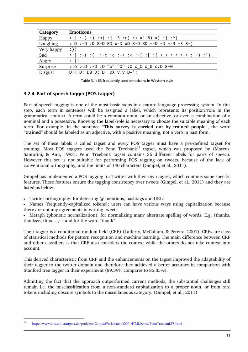
In this thesis, an emoticon library is created based on the suggestion from (Agarwal, Xie, Vovsha,

Rambow, & Passonneau, 2011). They are originally the smileys from Wikipedia11. This library has total

of 63 frequently used emoticons in Western style and they are described in the Table 3.1 below:

10

http://www.noslang.com/dictionary/full/ 11

http://en.wikipedia.org/wiki/List_of_emoticons

11

Category Emoticons

Happy >:] :-) :) :o) :] :3 :c) :> =] 8) =) :} :^)

Laughing >:D :-D :D 8-D 8D x-D xD X-D XD =-D =D =-3 =3 8-)

Very happy :))

Sad >:[ :-( :( :-c :c :-< :< :-[ :[ :{ >.> <.< >.< :'-) :')

Angry :-||

Surprise >:o >:O :-O :O °o° °O° :O o_O o_0 o.O 8-0

Disgust D:< D: D8 D; D= DX v.v D-':

Table 3.1: 63 frequently used emoticons in Western style

3.2.4. Part of speech tagger (POS-tagger)

Part of speech tagging is one of the most basic steps in a nature language processing system. In this

step, each term in sentences will be assigned a label, which represents its position/role in the

grammatical context. A term could be a common noun, or an adjective, or even a combination of a

nominal and a possessive. Knowing the label/role is necessary to choose the suitable meaning of each

term. For example, in the sentence “This survey is carried out by trained people”, the word “trained” should be labeled as an adjective, with a positive meaning, not a verb in past form.

The set of these labels is called tagset and every POS tagger must have a pre-defined tagset for

training. Most POS taggers used the Penn Treebank12 tagset, which was proposed by (Marcus,

Santorini, & Ann, 1993). Penn Treebank tagset contains 36 different labels for parts of speech.

However this set is not suitable for performing POS tagging on tweets, because of the lack of

conventional orthography, and the limits of 140 characters (Gimpel, et al., 2011).

Gimpel has implemented a POS tagging for Twitter with their own tagset, which contains some specific

features. These features ensure the tagging consistency over tweets (Gimpel, et al., 2011) and they are

listed as below:

Twitter orthography: for detecting @-mentions, hashtags and URLs

Names (frequently-capitalized tokens): users can have various ways using capitalization because

there are not any agreements in writing tweets

Metaph (phonetic normalization): for normalizing many alternate spelling of words. E.g. {thanks,

thanksss, thnx,…} stand for the word “thank”

Their tagger is a conditional random field (CRF) (Lafferty, McCallum, & Pereira, 2001). CRFs are class

of statistical methods for pattern recognition and machine learning. The main difference between CRF

and other classifiers is that CRF also considers the context while the others do not take context into

account.

This derived characteristic from CRF and the enhancements on the tagset improved the adaptability of

their tagger to the twitter domain and therefore they achieved a better accuracy in comparison with

Stanford tree tagger in their experiment (89.39% compares to 85.85%).

Admitting the fact that the approach outperformed current methods, the substantial challenges still

remain i.e. the misclassification from a non-standard capitalization to a proper noun, or from rare

tokens including obscure symbols to the miscellaneous category. (Gimpel, et al., 2011)

12

http://www.ims.uni-stuttgart.de/projekte/CorpusWorkbench/CQP-HTMLDemo/PennTreebankTS.html

12

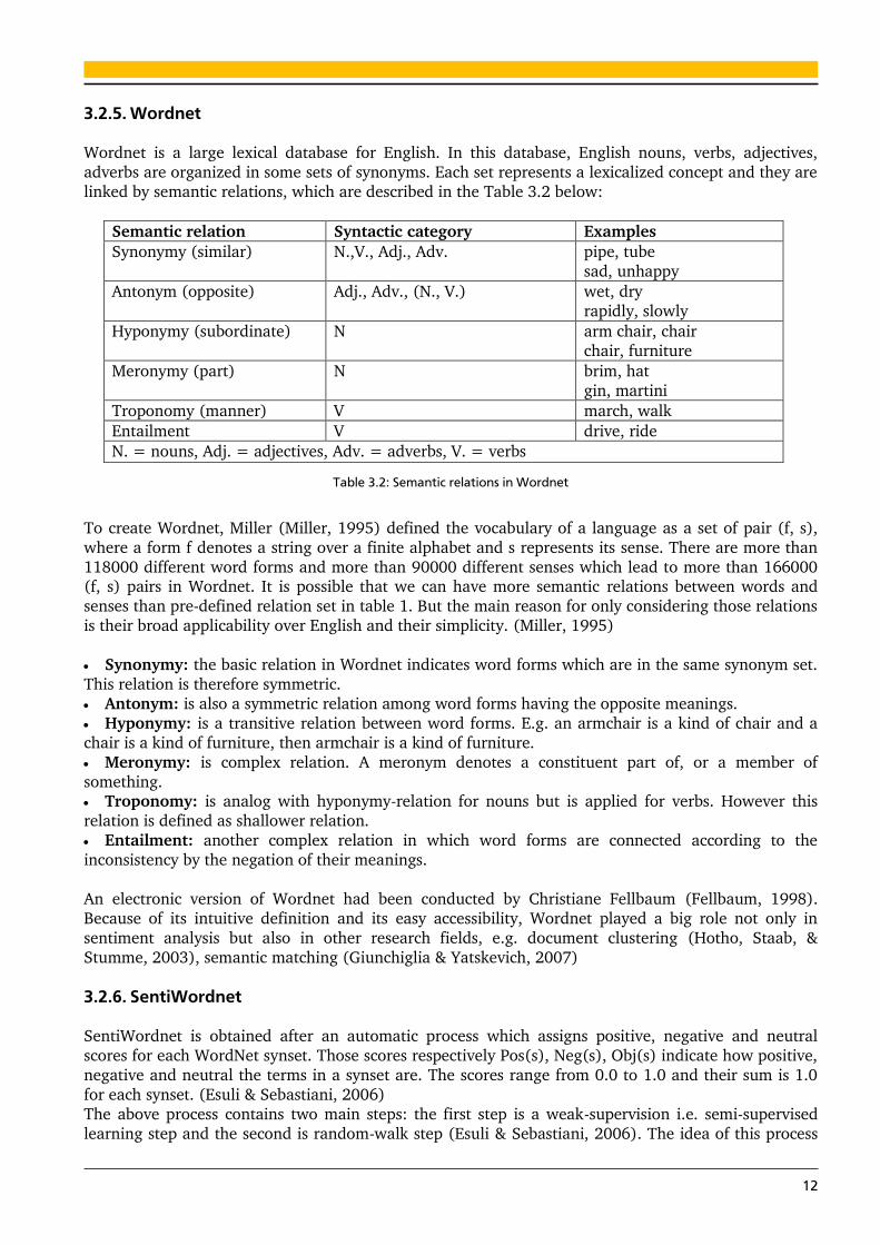
3.2.5. Wordnet

Wordnet is a large lexical database for English. In this database, English nouns, verbs, adjectives,

adverbs are organized in some sets of synonyms. Each set represents a lexicalized concept and they are

linked by semantic relations, which are described in the Table 3.2 below:

Semantic relation Syntactic category Examples

Synonymy (similar) N.,V., Adj., Adv. pipe, tube

sad, unhappy

Antonym (opposite) Adj., Adv., (N., V.) wet, dry

rapidly, slowly

Hyponymy (subordinate) N arm chair, chair

chair, furniture

Meronymy (part) N brim, hat

gin, martini

Troponomy (manner) V march, walk

Entailment V drive, ride

N. = nouns, Adj. = adjectives, Adv. = adverbs, V. = verbs

Table 3.2: Semantic relations in Wordnet

To create Wordnet, Miller (Miller, 1995) defined the vocabulary of a language as a set of pair (f, s),

where a form f denotes a string over a finite alphabet and s represents its sense. There are more than

118000 different word forms and more than 90000 different senses which lead to more than 166000 (f, s) pairs in Wordnet. It is possible that we can have more semantic relations between words and

senses than pre-defined relation set in table 1. But the main reason for only considering those relations

is their broad applicability over English and their simplicity. (Miller, 1995)

Synonymy: the basic relation in Wordnet indicates word forms which are in the same synonym set.

This relation is therefore symmetric.

Antonym: is also a symmetric relation among word forms having the opposite meanings.

Hyponymy: is a transitive relation between word forms. E.g. an armchair is a kind of chair and a

chair is a kind of furniture, then armchair is a kind of furniture.

Meronymy: is complex relation. A meronym denotes a constituent part of, or a member of

something. Troponomy: is analog with hyponymy-relation for nouns but is applied for verbs. However this

relation is defined as shallower relation.

Entailment: another complex relation in which word forms are connected according to the

inconsistency by the negation of their meanings.

An electronic version of Wordnet had been conducted by Christiane Fellbaum (Fellbaum, 1998).

Because of its intuitive definition and its easy accessibility, Wordnet played a big role not only in

sentiment analysis but also in other research fields, e.g. document clustering (Hotho, Staab, &

Stumme, 2003), semantic matching (Giunchiglia & Yatskevich, 2007)

3.2.6. SentiWordnet

SentiWordnet is obtained after an automatic process which assigns positive, negative and neutral

scores for each WordNet synset. Those scores respectively Pos(s), Neg(s), Obj(s) indicate how positive,

negative and neutral the terms in a synset are. The scores range from 0.0 to 1.0 and their sum is 1.0

for each synset. (Esuli & Sebastiani, 2006)

The above process contains two main steps: the first step is a weak-supervision i.e. semi-supervised

learning step and the second is random-walk step (Esuli & Sebastiani, 2006). The idea of this process

13

is based on a simple observation: if the terms used to describe a synset meaning are more likely to be

positive, then we have a high probability that this synset is positive. This observation leads to a graph-

based model on which the flow of positivity and negativity can be obtained by using several existing

graph algorithms.

3.2.7. DKPro

Many works have been conducted in Nature Language Processing (NLP) Community. One of them is

DKPro13. DKPro stands for Darmstadt Knowledge Processing Repository and is built based on

uimaFIT14. The main goal of this project is to provide a collection of components as well as third-party

tools, which cover the whole range of NLP-related tasks. With the integrated NLP tools in DKpro, the preprocessing steps like stemming, POS tagging are easily combined by adding the appropriate analysis

engine to the process pipeline.

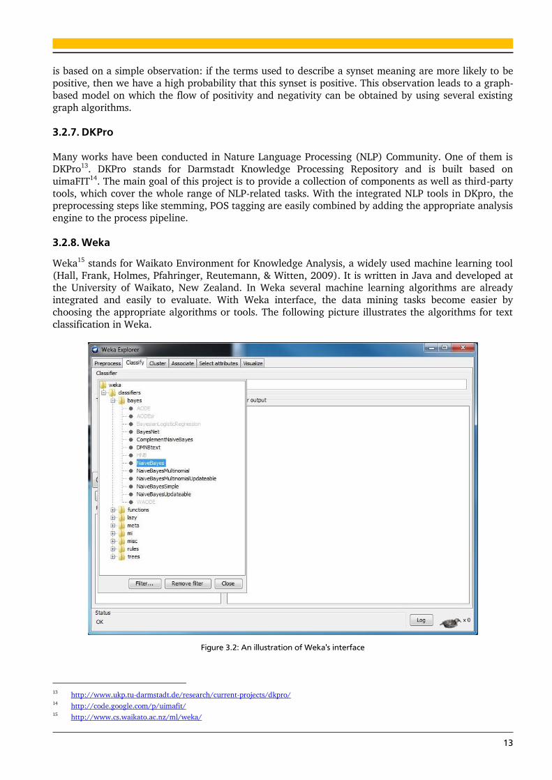
3.2.8. Weka

Weka15 stands for Waikato Environment for Knowledge Analysis, a widely used machine learning tool

(Hall, Frank, Holmes, Pfahringer, Reutemann, & Witten, 2009). It is written in Java and developed at the University of Waikato, New Zealand. In Weka several machine learning algorithms are already

integrated and easily to evaluate. With Weka interface, the data mining tasks become easier by

choosing the appropriate algorithms or tools. The following picture illustrates the algorithms for text

classification in Weka.

Figure 3.2: An illustration of Weka's interface

13

http://www.ukp.tu-darmstadt.de/research/current-projects/dkpro/ 14

http://code.google.com/p/uimafit/ 15

http://www.cs.waikato.ac.nz/ml/weka/

14

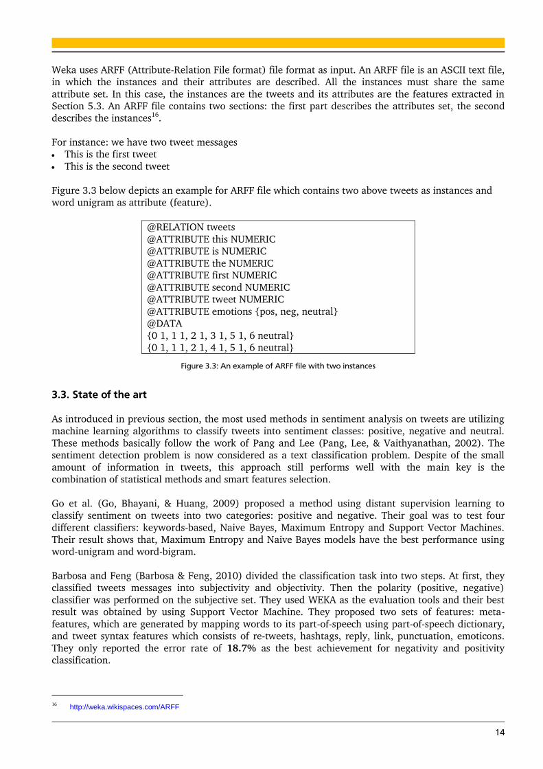
Weka uses ARFF (Attribute-Relation File format) file format as input. An ARFF file is an ASCII text file,

in which the instances and their attributes are described. All the instances must share the same

attribute set. In this case, the instances are the tweets and its attributes are the features extracted in

Section 5.3. An ARFF file contains two sections: the first part describes the attributes set, the second describes the instances16.

For instance: we have two tweet messages

This is the first tweet

This is the second tweet

Figure 3.3 below depicts an example for ARFF file which contains two above tweets as instances and

word unigram as attribute (feature).

@RELATION tweets

@ATTRIBUTE this NUMERIC

@ATTRIBUTE is NUMERIC

@ATTRIBUTE the NUMERIC @ATTRIBUTE first NUMERIC

@ATTRIBUTE second NUMERIC

@ATTRIBUTE tweet NUMERIC

@ATTRIBUTE emotions {pos, neg, neutral}

@DATA

{0 1, 1 1, 2 1, 3 1, 5 1, 6 neutral}

{0 1, 1 1, 2 1, 4 1, 5 1, 6 neutral}

Figure 3.3: An example of ARFF file with two instances

3.3. State of the art As introduced in previous section, the most used methods in sentiment analysis on tweets are utilizing

machine learning algorithms to classify tweets into sentiment classes: positive, negative and neutral.

These methods basically follow the work of Pang and Lee (Pang, Lee, & Vaithyanathan, 2002). The

sentiment detection problem is now considered as a text classification problem. Despite of the small

amount of information in tweets, this approach still performs well with the main key is the

combination of statistical methods and smart features selection.

Go et al. (Go, Bhayani, & Huang, 2009) proposed a method using distant supervision learning to

classify sentiment on tweets into two categories: positive and negative. Their goal was to test four

different classifiers: keywords-based, Naive Bayes, Maximum Entropy and Support Vector Machines.

Their result shows that, Maximum Entropy and Naive Bayes models have the best performance using word-unigram and word-bigram.

Barbosa and Feng (Barbosa & Feng, 2010) divided the classification task into two steps. At first, they

classified tweets messages into subjectivity and objectivity. Then the polarity (positive, negative)

classifier was performed on the subjective set. They used WEKA as the evaluation tools and their best

result was obtained by using Support Vector Machine. They proposed two sets of features: meta-

features, which are generated by mapping words to its part-of-speech using part-of-speech dictionary,

and tweet syntax features which consists of re-tweets, hashtags, reply, link, punctuation, emoticons.

They only reported the error rate of 18.7% as the best achievement for negativity and positivity

classification.

16

http://weka.wikispaces.com/ARFF

15

Agarwal et al. (Agarwal, Xie, Vovsha, Rambow, & Passonneau, 2011) used support vector machine

method, in which the unigram model and several features are incorporated. The features are number

of negation words, number of positive, negative words, number of extremely positive, extremely

negative, positive, negative emoticons, number of positive, negative hashtags, capitalized words and exclamation words. They achieved an accuracy of 75.39% using 5-fold cross validation on 2-way

classification task (only positive and negative), and an accuracy of 60.83% on the 3-way classification

task (neutral included) using these above listed features and partial tree kernel. The data set used for

evaluation contains 5127 tweets (1709 tweets for each class); it is acquired from a commercial source.

Kouloumpis et al. (Kouloumpis, Wilson, & Moore, 2011) investigated on a method that uses

BoosTexter17 with linguistic features for sentiment classification. They used the hashtagged data set

(HASH) from Edinburgh Twitter corpus18, and the emoticon data set (EMOT)19 for training purpose.

For evaluation, a manually annotated data set from iSieve Corporation is used. Their results are 74%

and 75% using only HASH, combination of HASH and EMOT as training data respectively. They

pointed out that the POS tagger might not be useful for sentiment analysis but also left a question on quality of their POS tagger while performing on tweets.

Jiang et al. (Jiang, Yu, Zhou, Liu, & Zhao, 2011) proposed to take the related messages of the current

tweet in order to improve the performance. They also extended the popular features set by target-

dependent features. Those features are generated by analyzing verbs, adverbs and adjectives in tweets.

Their method was based on a hypothesis, that a direct comment about functionalities of a product also

affects the opinion about it. For example: "I very like Microsoft technologies" expresses directly a

positive sentiment about Microsoft technologies but also implies a positive sentiment about Microsoft.

Their data set for evaluation thus contains only tweet messages about some specific targets. Five

popular topics are used: {Obama, Google, iPad, Lakers, Lady Gaga}. They reported a result of 85.6%

accuracy by classifying tweets polarity from a set of 268 each randomly selected negative and positive tweets (536 totals). They also achieved a better percentage using the related tweets graph from 66.0%

to 68.3% accuracy in 3-ways classification task (pos-, negative, neutral).The related tweets graph is

obtained by taking retweet, reply, tweet of same people into account. Support Vector Machine is used

in this work in order to classify tweets into subjective and objective class, and then to map the tweets

from subjective class to negative or positive respectively.

Saif et al. (Saif, He, & Alani, 2012) introduced an interesting methods using Naive Bayes classifier.

They extract the named entities in tweet messages, e.g. "Iphone", "Ipad"... and replace them by their

corresponding concepts "Apple/Product". The concepts are extracted from the corpus using

AlchemyAPI20. They then incorporate these semantic concepts and their distribution in training phases

and report an accuracy of 86.3% on their extended Stanford Twitter Sentiment Data set with 527 negative and 473 positive tweet messages (The original test set contains only 177 negative and 182

positive tweets). This method alleviates the data's sparsity and thus reduces the number of features in

training and classification phases.

Nagy and Stammberger (Nagy & Stammberger, 2012) used a simple method to detect sentiment in

tweets. They calculated the sentiment value for each tweets using the number of positive and negative

word. In their approach, the AFINN word list and the SentiWordnet are used to detect positive- and

negative sentiment value for each word/token.

∑

17

http://www.cs.princeton.edu/~schapire/boostexter.html 18

http://demeter.inf.ed.ac.uk 19

http://twittersentiment.appspot.com 20

http://www.alchemyapi.com/

16

Where:

is number of words with positive sentiment value

is number of words with negative sentiment value

n is total number of lexicons in a Tweet

As the second method, they used the normalized value calculated by:

and combined those two values with the result from Bayesian Classifier to obtain the result class for

each tweets. A recall value of 0.96 and precision value of 0.94 are achieved. These values lead to an F-

Measure value of 0.94.

For evaluation purpose, they used TwapperKeeper21 with the keywords #sanbrunofire and sanbrunofire

to collect 3698 tweets in the first 24 hours after San Bruno event22. Those collected tweets are

manually annotated using Crowdflower23, a crowd sourcing system.

Their approach is a good sample for opinion detection during disaster and crises. However, only small

amount of those tweets contains sentiment (39% for the tweets collected after 12 hours, and 54% in the rest 12 hours). It leads to a baseline of 61% in the first half by automatically assigning neutral label

for all tweets.

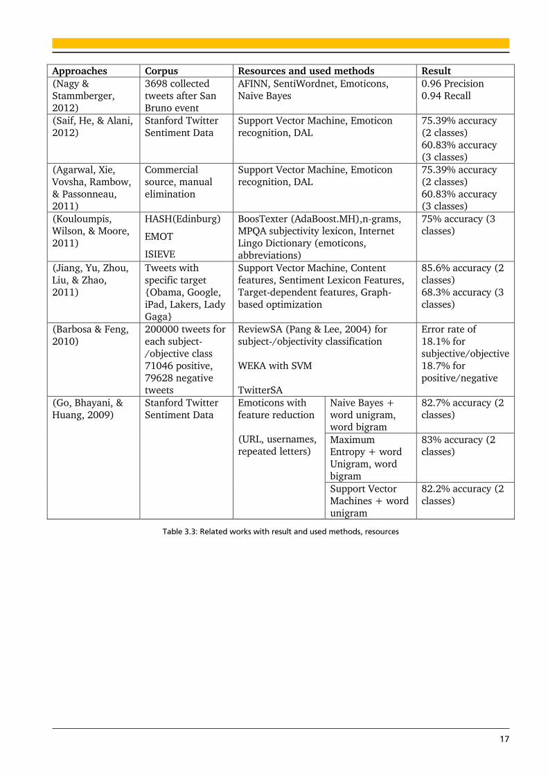
The following table sums up all the achieved results with used methods and resources. The comparison

of those approaches is difficult because of different corpora which they used to test.

21

www.twapperkkeeper.com 22

http://en.wikipedia.org/wiki/2010_San_Bruno_pipeline_explosion 23

www.crowdflower.com

17

Approaches Corpus Resources and used methods Result

(Nagy &

Stammberger,

2012)

3698 collected

tweets after San

Bruno event

AFINN, SentiWordnet, Emoticons,

Naive Bayes

0.96 Precision

0.94 Recall

(Saif, He, & Alani,

2012)

Stanford Twitter

Sentiment Data

Support Vector Machine, Emoticon

recognition, DAL

75.39% accuracy

(2 classes)

60.83% accuracy

(3 classes)

(Agarwal, Xie,

Vovsha, Rambow,

& Passonneau, 2011)

Commercial

source, manual

elimination

Support Vector Machine, Emoticon

recognition, DAL

75.39% accuracy

(2 classes)

60.83% accuracy (3 classes)

(Kouloumpis, Wilson, & Moore,

2011)

HASH(Edinburg)

EMOT

ISIEVE

BoosTexter (AdaBoost.MH),n-grams, MPQA subjectivity lexicon, Internet

Lingo Dictionary (emoticons,

abbreviations)

75% accuracy (3 classes)

(Jiang, Yu, Zhou,

Liu, & Zhao,

2011)

Tweets with

specific target

{Obama, Google,

iPad, Lakers, Lady

Gaga}

Support Vector Machine, Content

features, Sentiment Lexicon Features,

Target-dependent features, Graph-

based optimization

85.6% accuracy (2

classes)

68.3% accuracy (3

classes)

(Barbosa & Feng,

2010)

200000 tweets for

each subject-

/objective class

71046 positive,

79628 negative

tweets

ReviewSA (Pang & Lee, 2004) for

subject-/objectivity classification

WEKA with SVM

TwitterSA

Error rate of

18.1% for

subjective/objective

18.7% for

positive/negative

(Go, Bhayani, &

Huang, 2009)

Stanford Twitter

Sentiment Data

Emoticons with

feature reduction

(URL, usernames,

repeated letters)

Naive Bayes +

word unigram, word bigram

82.7% accuracy (2

classes)

Maximum Entropy + word

Unigram, word

bigram

83% accuracy (2 classes)

Support Vector

Machines + word

unigram

82.2% accuracy (2

classes)

Table 3.3: Related works with result and used methods, resources

18

4. Experiment setup

This section probes into the surveys for obtaining the data sets in different geographic territory during

specified time period. Those data sets will be used to evaluate the different algorithms, which are

described in Section 6.

It should be noted that, the experiment consists of two different classification problems. The first one

called 3-classes problem is to determine if a tweet belongs to positive, negative or neutral class. Two

data sets are used for this problem (SET3_GP, SET4). The other called 7-classes problem is to classify

tweets into seven concrete emotion categories according to Ekman’s work (Ekman, 1992). In this

problem, three data sets named SET1, SET2, and SET3 are used for evaluation.

4.1. Data sets

Initially, the first data set contained 200 tweets in English, which have been collected from the users in

Seattle from 08:23, March, 06 2012 to 18:12 March, 06 2012. The second set also contains 200

tweets but all of them are in Vietnamese in order to evaluate the performance of approaches with

different languages. Those Vietnamese tweets are generated by different users in Hanoi, and collected

from 14:28 March, 23 2012 to 15:08 March, 23 2012.

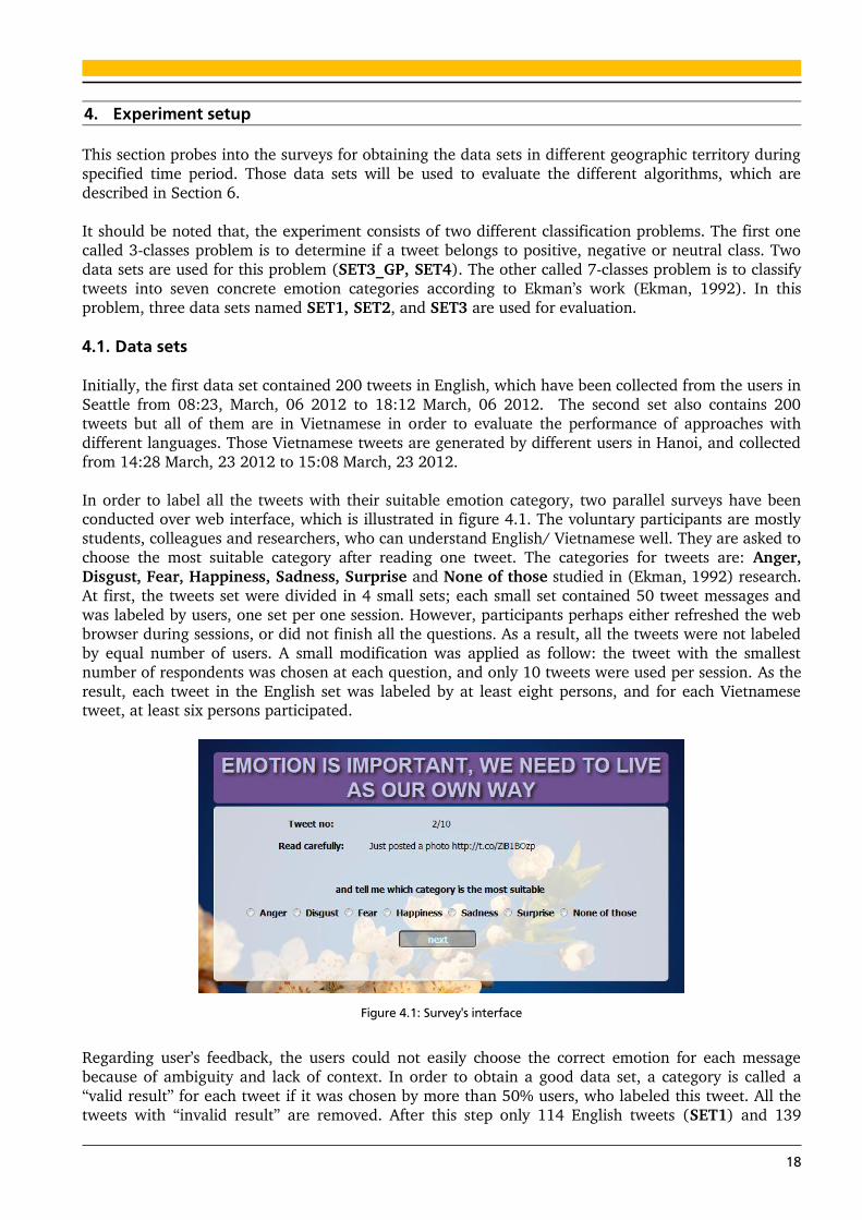
In order to label all the tweets with their suitable emotion category, two parallel surveys have been conducted over web interface, which is illustrated in figure 4.1. The voluntary participants are mostly

students, colleagues and researchers, who can understand English/ Vietnamese well. They are asked to

choose the most suitable category after reading one tweet. The categories for tweets are: Anger, Disgust, Fear, Happiness, Sadness, Surprise and None of those studied in (Ekman, 1992) research.

At first, the tweets set were divided in 4 small sets; each small set contained 50 tweet messages and

was labeled by users, one set per one session. However, participants perhaps either refreshed the web

browser during sessions, or did not finish all the questions. As a result, all the tweets were not labeled

by equal number of users. A small modification was applied as follow: the tweet with the smallest

number of respondents was chosen at each question, and only 10 tweets were used per session. As the

result, each tweet in the English set was labeled by at least eight persons, and for each Vietnamese tweet, at least six persons participated.

Figure 4.1: Survey's interface

Regarding user’s feedback, the users could not easily choose the correct emotion for each message

because of ambiguity and lack of context. In order to obtain a good data set, a category is called a

“valid result” for each tweet if it was chosen by more than 50% users, who labeled this tweet. All the

tweets with “invalid result” are removed. After this step only 114 English tweets (SET1) and 139

19

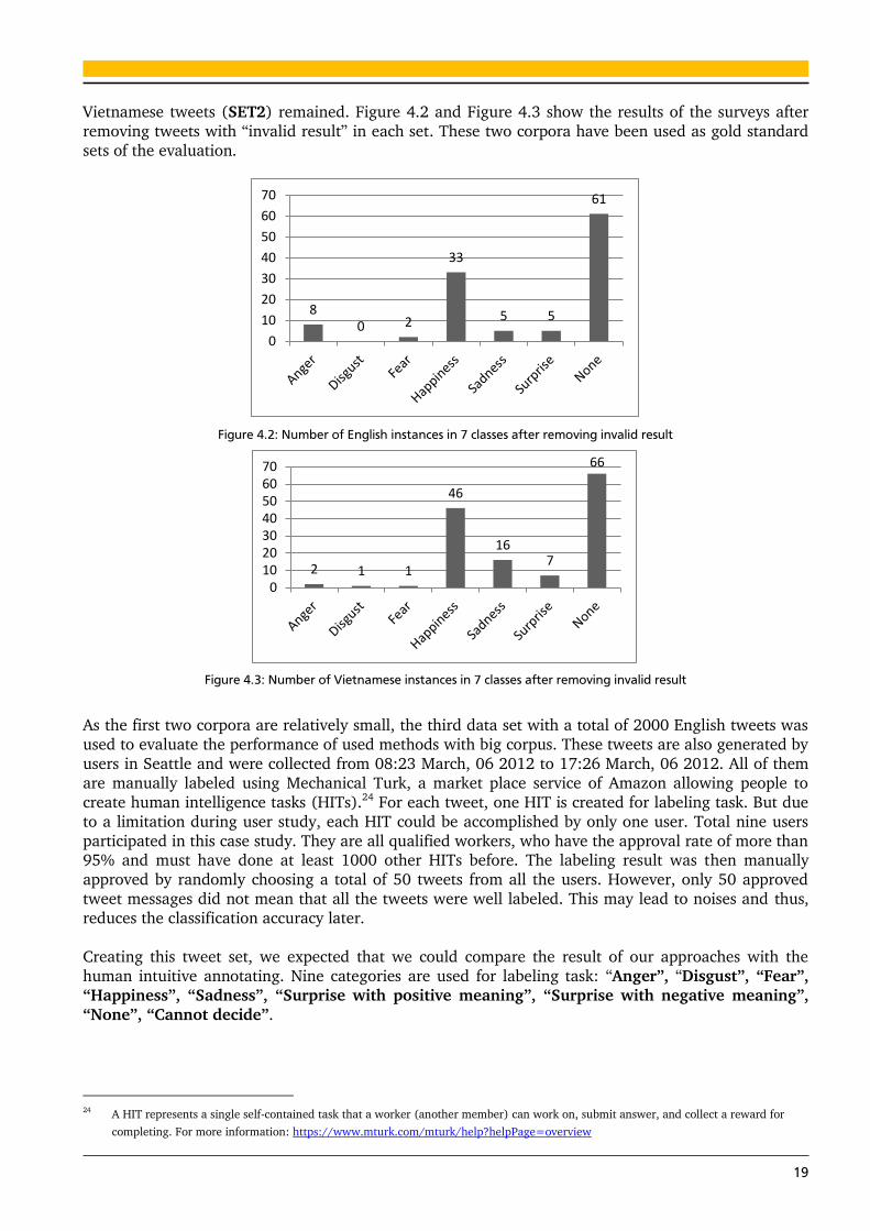
Vietnamese tweets (SET2) remained. Figure 4.2 and Figure 4.3 show the results of the surveys after

removing tweets with “invalid result” in each set. These two corpora have been used as gold standard

sets of the evaluation.

Figure 4.2: Number of English instances in 7 classes after removing invalid result

Figure 4.3: Number of Vietnamese instances in 7 classes after removing invalid result

As the first two corpora are relatively small, the third data set with a total of 2000 English tweets was

used to evaluate the performance of used methods with big corpus. These tweets are also generated by

users in Seattle and were collected from 08:23 March, 06 2012 to 17:26 March, 06 2012. All of them

are manually labeled using Mechanical Turk, a market place service of Amazon allowing people to

create human intelligence tasks (HITs).24 For each tweet, one HIT is created for labeling task. But due

to a limitation during user study, each HIT could be accomplished by only one user. Total nine users

participated in this case study. They are all qualified workers, who have the approval rate of more than 95% and must have done at least 1000 other HITs before. The labeling result was then manually

approved by randomly choosing a total of 50 tweets from all the users. However, only 50 approved

tweet messages did not mean that all the tweets were well labeled. This may lead to noises and thus,

reduces the classification accuracy later.

Creating this tweet set, we expected that we could compare the result of our approaches with the

human intuitive annotating. Nine categories are used for labeling task: “Anger”, “Disgust”, “Fear”, “Happiness”, “Sadness”, “Surprise with positive meaning”, “Surprise with negative meaning”, “None”, “Cannot decide”.

24

A HIT represents a single self-contained task that a worker (another member) can work on, submit answer, and collect a reward for

completing. For more information: https://www.mturk.com/mturk/help?helpPage=overview

8 0 2

33

5 5

61

0

10

20

30

40

50

60

70

2 1 1

46

16 7

66

010203040506070

20

In comparison with the first two data sets, we added the “Cannot decide” category, and divided

“Surprise” into two sub-categories: “Surprise with positive meaning” and “Surprise with negative meaning”.

The “Cannot decide” category is added to prevent the case user cannot choose the right emotion of

tweet’s author. All the tweets in this category (49 tweets total) are then removed.

The reason of dividing “Surprise” into two sub-categories is: when a user is surprised about

something, it could be a positive or negative emotion. After this step, we could easily reorganize these

eight categories into three classes: positive, negative, neutral by grouping “Disgust”, “Fear”, “Sadness”, “Surprise with negative meaning” into negative class, “Happiness”, “Surprise with positive meaning” into positive class, and “None” into neutral class. This tweak will allow us to use

this data set for 3-classes problem.

There are 24 tweets belong to “Surprise with positive meaning”, and 30 tweets belong to “Surprise with negative meaning”.

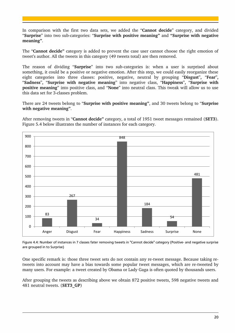
After removing tweets in “Cannot decide” category, a total of 1951 tweet messages remained (SET3).

Figure 5.4 below illustrates the number of instances for each category.

Figure 4.4: Number of instances in 7 classes fater removing tweets in "Cannot decide" category (Positive- and negative surprise

are grouped in to Surprise)

One specific remark is: those three tweet sets do not contain any re-tweet message. Because taking re-

tweets into account may have a bias towards some popular tweet messages, which are re-tweeted by

many users. For example: a tweet created by Obama or Lady Gaga is often quoted by thousands users.

After grouping the tweets as describing above we obtain 872 positive tweets, 598 negative tweets and

481 neutral tweets. (SET3_GP)

83

267

34

848

184

54

481

0

100

200

300

400

500

600

700

800

900

Anger Disgust Fear Happiness Sadness Surprise None

21

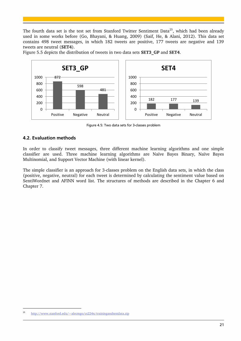
The fourth data set is the test set from Stanford Twitter Sentiment Data25, which had been already

used in some works before (Go, Bhayani, & Huang, 2009) (Saif, He, & Alani, 2012). This data set

contains 498 tweet messages, in which 182 tweets are positive, 177 tweets are negative and 139

tweets are neutral (SET4). Figure 5.5 depicts the distribution of tweets in two data sets SET3_GP and SET4.

Figure 4.5: Two data sets for 3-classes problem

4.2. Evaluation methods

In order to classify tweet messages, three different machine learning algorithms and one simple

classifier are used. Three machine learning algorithms are Naïve Bayes Binary, Naïve Bayes

Multinomial, and Support Vector Machine (with linear kernel).

The simple classifier is an approach for 3-classes problem on the English data sets, in which the class

(positive, negative, neutral) for each tweet is determined by calculating the sentiment value based on

SentiWordnet and AFINN word list. The structures of methods are described in the Chapter 6 and

Chapter 7.

25

http://www.stanford.edu/~alecmgo/cs224n/trainingandtestdata.zip

872

598 481

0

200

400

600

800

1000

Positive Negative Neutral

SET3_GP

182 177 139

0

200

400

600

800

1000

Positive Negative Neutral

SET4

22

5. Evaluation methods for English data sets

In this section, several approaches in order to classify English tweets into different emotion categories

are described.

5.1. Structure of evaluation methods for English data sets

After the tweets labeling phase was finished, the data sets, with each two lines containing a tweets and

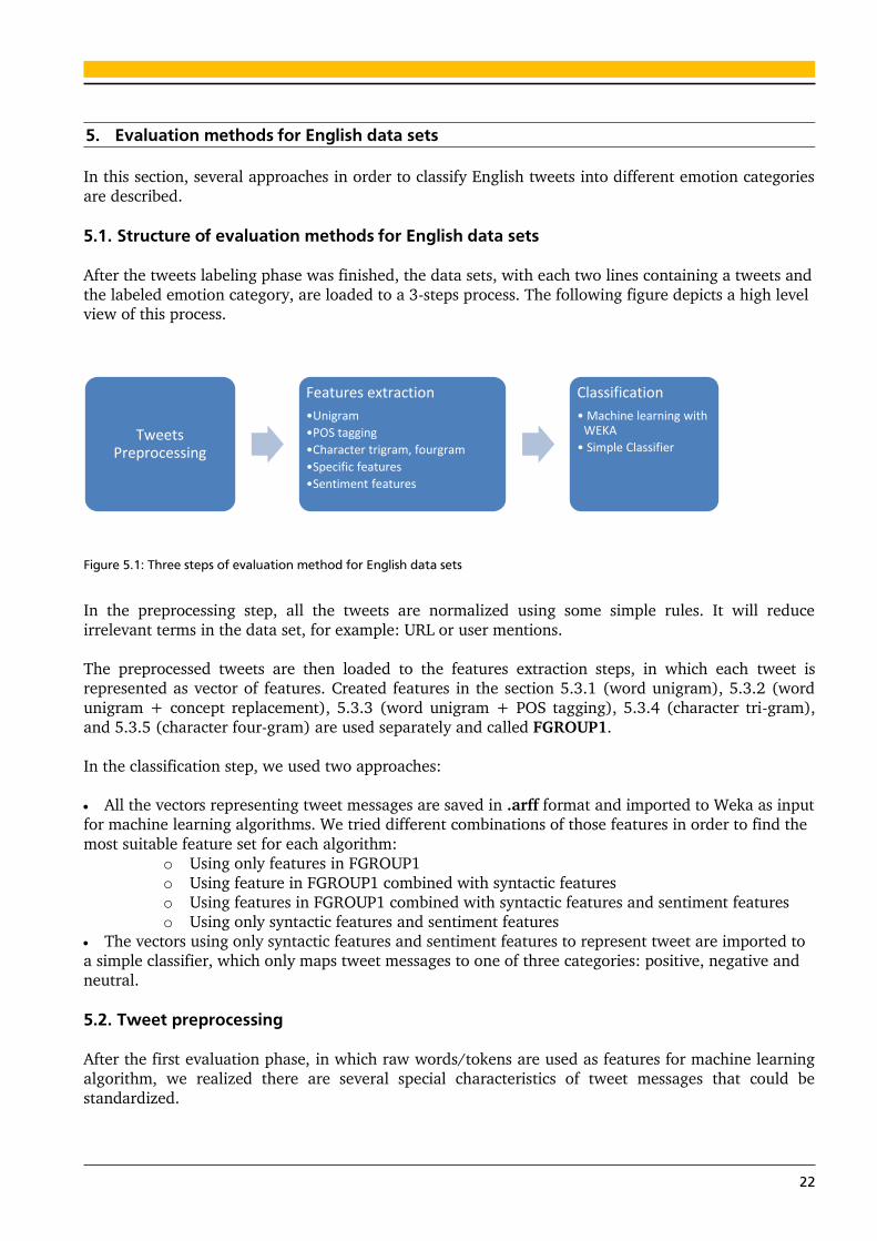
the labeled emotion category, are loaded to a 3-steps process. The following figure depicts a high level view of this process.

Figure 5.1: Three steps of evaluation method for English data sets

In the preprocessing step, all the tweets are normalized using some simple rules. It will reduce

irrelevant terms in the data set, for example: URL or user mentions.

The preprocessed tweets are then loaded to the features extraction steps, in which each tweet is

represented as vector of features. Created features in the section 5.3.1 (word unigram), 5.3.2 (word

unigram + concept replacement), 5.3.3 (word unigram + POS tagging), 5.3.4 (character tri-gram),

and 5.3.5 (character four-gram) are used separately and called FGROUP1.

In the classification step, we used two approaches:

All the vectors representing tweet messages are saved in .arff format and imported to Weka as input

for machine learning algorithms. We tried different combinations of those features in order to find the

most suitable feature set for each algorithm:

o Using only features in FGROUP1

o Using feature in FGROUP1 combined with syntactic features

o Using features in FGROUP1 combined with syntactic features and sentiment features

o Using only syntactic features and sentiment features

The vectors using only syntactic features and sentiment features to represent tweet are imported to

a simple classifier, which only maps tweet messages to one of three categories: positive, negative and

neutral.

5.2. Tweet preprocessing

After the first evaluation phase, in which raw words/tokens are used as features for machine learning

algorithm, we realized there are several special characteristics of tweet messages that could be

standardized.

Tweets Preprocessing

Features extraction

•Unigram

•POS tagging

•Character trigram, fourgram

•Specific features

•Sentiment features

Classification

• Machine learning with WEKA

• Simple Classifier

23

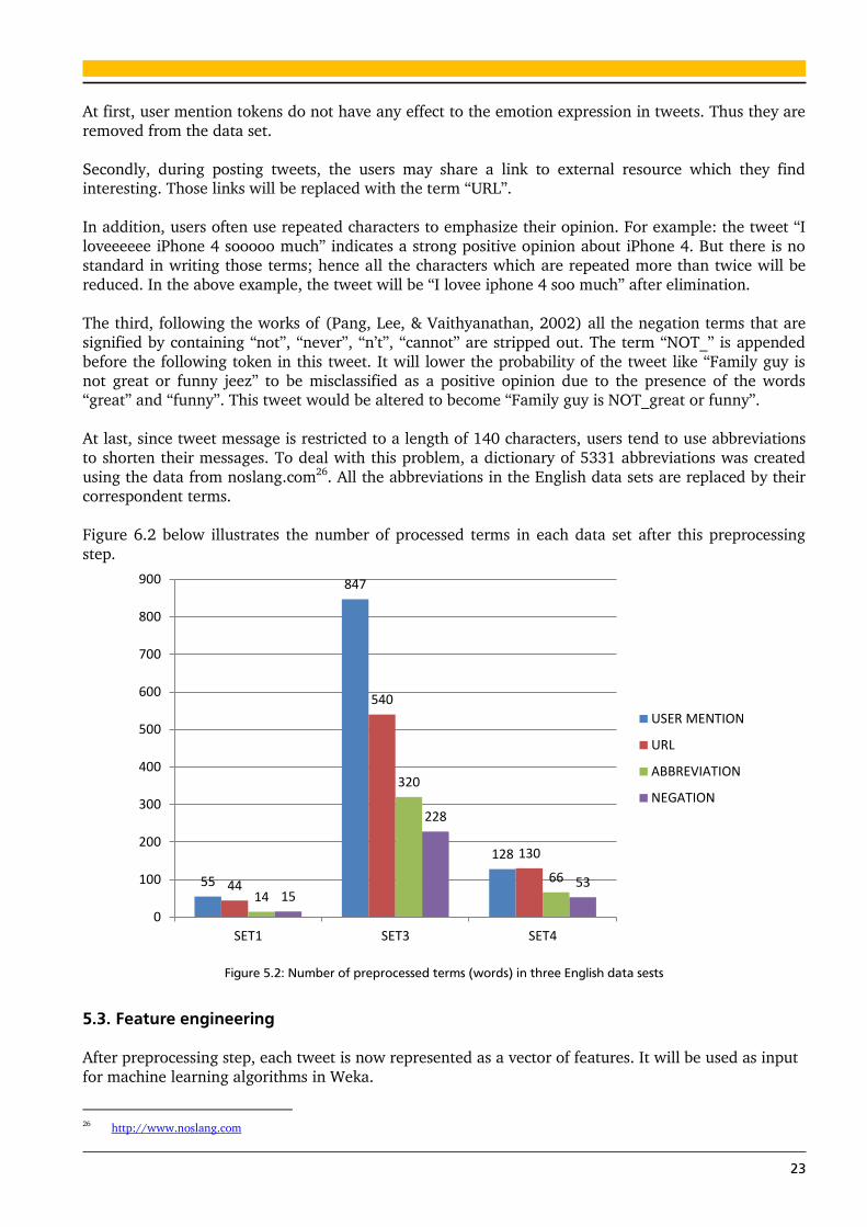
At first, user mention tokens do not have any effect to the emotion expression in tweets. Thus they are

removed from the data set.

Secondly, during posting tweets, the users may share a link to external resource which they find interesting. Those links will be replaced with the term “URL”.

In addition, users often use repeated characters to emphasize their opinion. For example: the tweet “I

loveeeeee iPhone 4 sooooo much” indicates a strong positive opinion about iPhone 4. But there is no

standard in writing those terms; hence all the characters which are repeated more than twice will be

reduced. In the above example, the tweet will be “I lovee iphone 4 soo much” after elimination.

The third, following the works of (Pang, Lee, & Vaithyanathan, 2002) all the negation terms that are

signified by containing “not”, “never”, “n’t”, “cannot” are stripped out. The term “NOT_” is appended

before the following token in this tweet. It will lower the probability of the tweet like “Family guy is

not great or funny jeez” to be misclassified as a positive opinion due to the presence of the words “great” and “funny”. This tweet would be altered to become “Family guy is NOT_great or funny”.

At last, since tweet message is restricted to a length of 140 characters, users tend to use abbreviations

to shorten their messages. To deal with this problem, a dictionary of 5331 abbreviations was created

using the data from noslang.com26. All the abbreviations in the English data sets are replaced by their

correspondent terms.

Figure 6.2 below illustrates the number of processed terms in each data set after this preprocessing

step.

Figure 5.2: Number of preprocessed terms (words) in three English data sests

5.3. Feature engineering

After preprocessing step, each tweet is now represented as a vector of features. It will be used as input

for machine learning algorithms in Weka.

26

http://www.noslang.com

55

847

128

44

540

130

14

320

66

15

228

53

0

100

200

300

400

500

600

700

800

900

SET1 SET3 SET4

USER MENTION

URL

ABBREVIATION

NEGATION

24

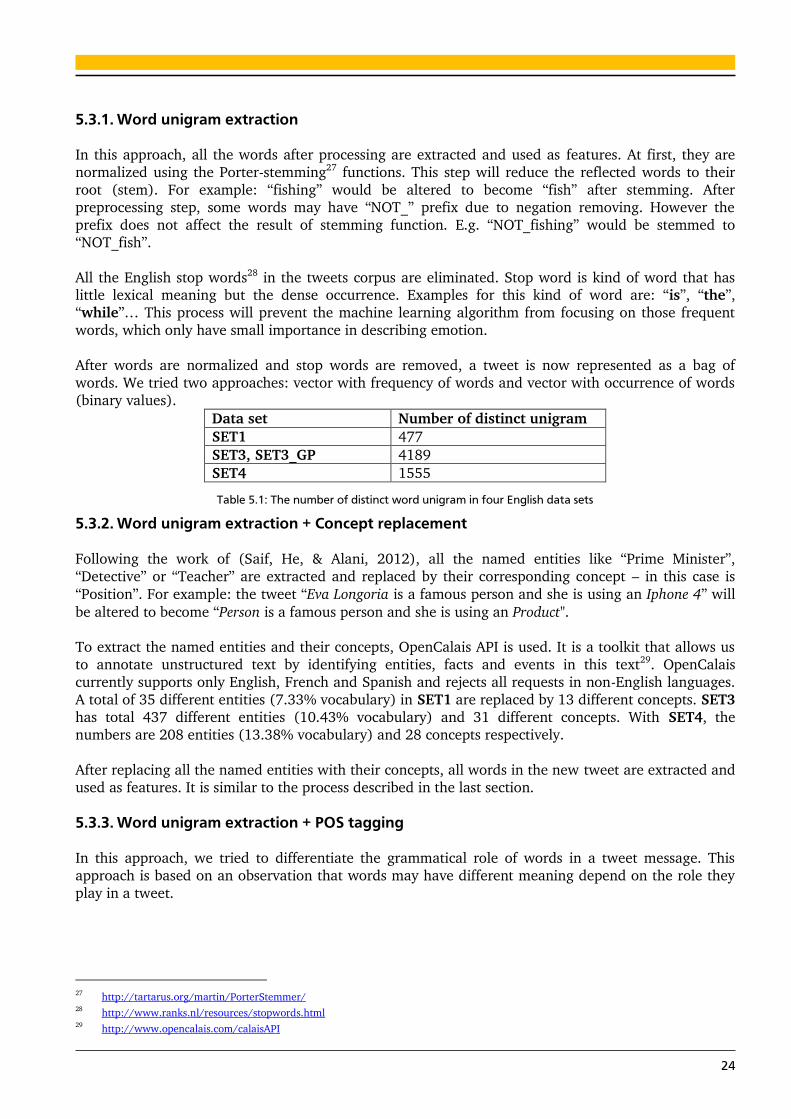
5.3.1. Word unigram extraction

In this approach, all the words after processing are extracted and used as features. At first, they are

normalized using the Porter-stemming27 functions. This step will reduce the reflected words to their

root (stem). For example: “fishing” would be altered to become “fish” after stemming. After

preprocessing step, some words may have “NOT_” prefix due to negation removing. However the

prefix does not affect the result of stemming function. E.g. “NOT_fishing” would be stemmed to

“NOT_fish”.

All the English stop words28 in the tweets corpus are eliminated. Stop word is kind of word that has little lexical meaning but the dense occurrence. Examples for this kind of word are: “is”, “the”,

“while”… This process will prevent the machine learning algorithm from focusing on those frequent

words, which only have small importance in describing emotion.

After words are normalized and stop words are removed, a tweet is now represented as a bag of

words. We tried two approaches: vector with frequency of words and vector with occurrence of words

(binary values).

Data set Number of distinct unigram

SET1 477

SET3, SET3_GP 4189

SET4 1555

Table 5.1: The number of distinct word unigram in four English data sets

5.3.2. Word unigram extraction + Concept replacement

Following the work of (Saif, He, & Alani, 2012), all the named entities like “Prime Minister”,

“Detective” or “Teacher” are extracted and replaced by their corresponding concept – in this case is

“Position”. For example: the tweet “Eva Longoria is a famous person and she is using an Iphone 4” will

be altered to become “Person is a famous person and she is using an Product".

To extract the named entities and their concepts, OpenCalais API is used. It is a toolkit that allows us

to annotate unstructured text by identifying entities, facts and events in this text29. OpenCalais

currently supports only English, French and Spanish and rejects all requests in non-English languages.

A total of 35 different entities (7.33% vocabulary) in SET1 are replaced by 13 different concepts. SET3

has total 437 different entities (10.43% vocabulary) and 31 different concepts. With SET4, the

numbers are 208 entities (13.38% vocabulary) and 28 concepts respectively.

After replacing all the named entities with their concepts, all words in the new tweet are extracted and

used as features. It is similar to the process described in the last section.

5.3.3. Word unigram extraction + POS tagging

In this approach, we tried to differentiate the grammatical role of words in a tweet message. This

approach is based on an observation that words may have different meaning depend on the role they

play in a tweet.

27

http://tartarus.org/martin/PorterStemmer/ 28

http://www.ranks.nl/resources/stopwords.html 29

http://www.opencalais.com/calaisAPI

25

We applied two different POS-taggers to assign POS-label to each word in three English sets. One is

TT4J-Tagger (TreeTagger for Java)30. This Tree Tagger is already integrated in DKPro. The second

POS-Tagger is the proposed POS-Tagger from (Gimpel, et al., 2011). Although the second POS-Tagger

is more suitable for tweet corpus, applying it on our data set showed timing issue. Thus, the first POS-tagger is chosen for the labeling task.

In order to incorporate different roles of words into training phase, the POS-label of a word is

appended before it. The concatenation of POS-label and the original word is considered as feature

instead of using the word only.

For example: if the tweet message is: “So happy, I don’t have to set my alarm tonight!! lol”. The tagged

tweet would be “RB_so JJ_happy PP_I VVD_don’t VH_have TO_to VV_set PP$_my NN_alarm NN_tonight

SENT_! SENT_! NN_lol”. RB, JJ, PP, VD, etc. are the correspondence POS-labels for each word from the TT4J-Tagger.

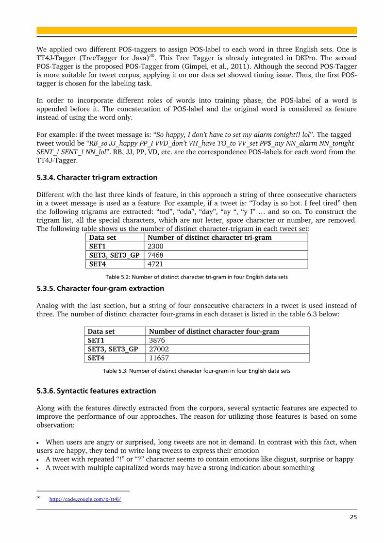
5.3.4. Character tri-gram extraction

Different with the last three kinds of feature, in this approach a string of three consecutive characters in a tweet message is used as a feature. For example, if a tweet is: “Today is so hot. I feel tired” then

the following trigrams are extracted: “tod”, “oda”, “day”, “ay “, “y I” … and so on. To construct the

trigram list, all the special characters, which are not letter, space character or number, are removed.

The following table shows us the number of distinct character-trigram in each tweet set:

Data set Number of distinct character tri-gram

SET1 2300

SET3, SET3_GP 7468

SET4 4721

Table 5.2: Number of distinct character tri-gram in four English data sets

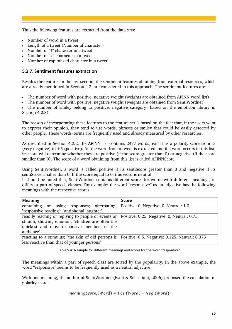
5.3.5. Character four-gram extraction

Analog with the last section, but a string of four consecutive characters in a tweet is used instead of

three. The number of distinct character four-grams in each dataset is listed in the table 6.3 below:

Data set Number of distinct character four-gram

SET1 3876

SET3, SET3_GP 27002

SET4 11657

Table 5.3: Number of distinct character four-gram in four English data sets

5.3.6. Syntactic features extraction Along with the features directly extracted from the corpora, several syntactic features are expected to

improve the performance of our approaches. The reason for utilizing those features is based on some

observation:

When users are angry or surprised, long tweets are not in demand. In contrast with this fact, when

users are happy, they tend to write long tweets to express their emotion

A tweet with repeated “!” or “?” character seems to contain emotions like disgust, surprise or happy

A tweet with multiple capitalized words may have a strong indication about something

30

http://code.google.com/p/tt4j/

26

Thus the following features are extracted from the data sets:

Number of word in a tweet

Length of a tweet (Number of character) Number of “!” character in a tweet

Number of “?” character in a tweet

Number of capitalized character in a tweet

5.3.7. Sentiment features extraction

Besides the features in the last section, the sentiment features obtaining from external resources, which are already mentioned in Section 4.2, are considered in this approach. The sentiment features are:

The number of word with positive, negative weight (weights are obtained from AFINN word list)

The number of word with positive, negative weight (weights are obtained from SentiWordnet)

The number of smiley belong to positive, negative category (based on the emoticon library in

Section 4.2.3)

The reason of incorporating these features to the feature set is based on the fact that, if the users want

to express their opinion, they tend to use words, phrases or smiley that could be easily detected by

other people. These words/terms are frequently used and already measured by other researches.

As described in Section 4.2.2, the AFINN list contains 2477 words; each has a polarity score from -5

(very negative) to +5 (positive). All the word from a tweet is extracted and if a word occurs in this list,

its score will determine whether they are positive (if the score greater than 0) or negative (if the score

smaller than 0). The score of a word obtaining from this list is called AFINNScore.

Using SentiWordnet, a word is called positive if its sentiScore greater than 0 and negative if its

sentiScore smaller than 0. If the score equal to 0, this word is neutral.

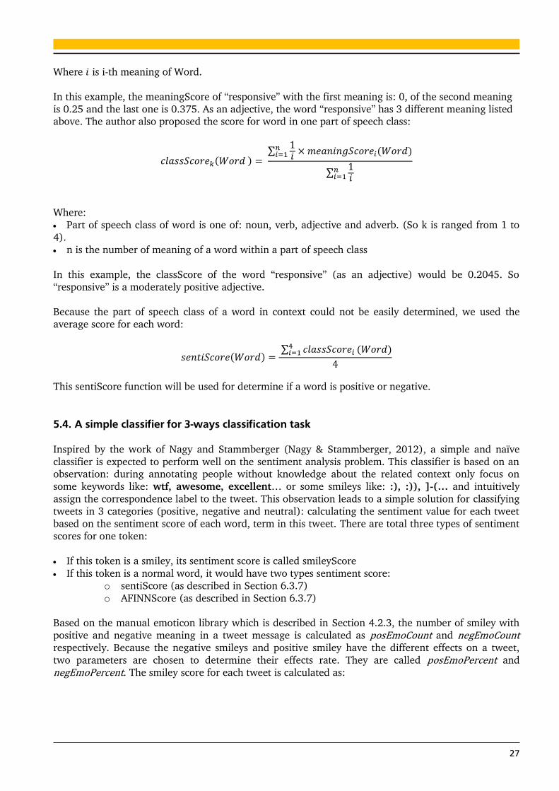
It should be noted that, SentiWordnet contains different scores for words with different meanings, in

different part of speech classes. For example: the word “responsive” as an adjective has the following

meanings with the respective scores:

Meaning Score

containing or using responses; alternating;

"responsive reading"; "antiphonal laughter"

Positive: 0, Negative: 0, Neutral: 1.0

readily reacting or replying to people or events or

stimuli; showing emotion; "children are often the quickest and most responsive members of the

audience"

Positive: 0.25, Negative: 0, Neutral: 0.75

reacting to a stimulus; "the skin of old persons is

less reactive than that of younger persons"

Positive: 0.5, Negative: 0.125, Neutral: 0.375

Table 5.4: A sample for different meanings and scores for the word "responsive"

The meanings within a part of speech class are sorted by the popularity. In the above example, the

word “responsive” seems to be frequently used as a neutral adjective.

With one meaning, the author of SentiWordnet (Esuli & Sebastiani, 2006) proposed the calculation of

polarity score:

27

Where is i-th meaning of Word.

In this example, the meaningScore of “responsive” with the first meaning is: 0, of the second meaning

is 0.25 and the last one is 0.375. As an adjective, the word “responsive” has 3 different meaning listed above. The author also proposed the score for word in one part of speech class:

∑

∑

Where:

Part of speech class of word is one of: noun, verb, adjective and adverb. (So k is ranged from 1 to

4).

n is the number of meaning of a word within a part of speech class

In this example, the classScore of the word “responsive” (as an adjective) would be 0.2045. So

“responsive” is a moderately positive adjective.

Because the part of speech class of a word in context could not be easily determined, we used the

average score for each word:

∑

This sentiScore function will be used for determine if a word is positive or negative.

5.4. A simple classifier for 3-ways classification task

Inspired by the work of Nagy and Stammberger (Nagy & Stammberger, 2012), a simple and naïve

classifier is expected to perform well on the sentiment analysis problem. This classifier is based on an observation: during annotating people without knowledge about the related context only focus on

some keywords like: wtf, awesome, excellent… or some smileys like: :), :)), ]-(… and intuitively

assign the correspondence label to the tweet. This observation leads to a simple solution for classifying

tweets in 3 categories (positive, negative and neutral): calculating the sentiment value for each tweet

based on the sentiment score of each word, term in this tweet. There are total three types of sentiment

scores for one token:

If this token is a smiley, its sentiment score is called smileyScore

If this token is a normal word, it would have two types sentiment score:

o sentiScore (as described in Section 6.3.7)

o AFINNScore (as described in Section 6.3.7)

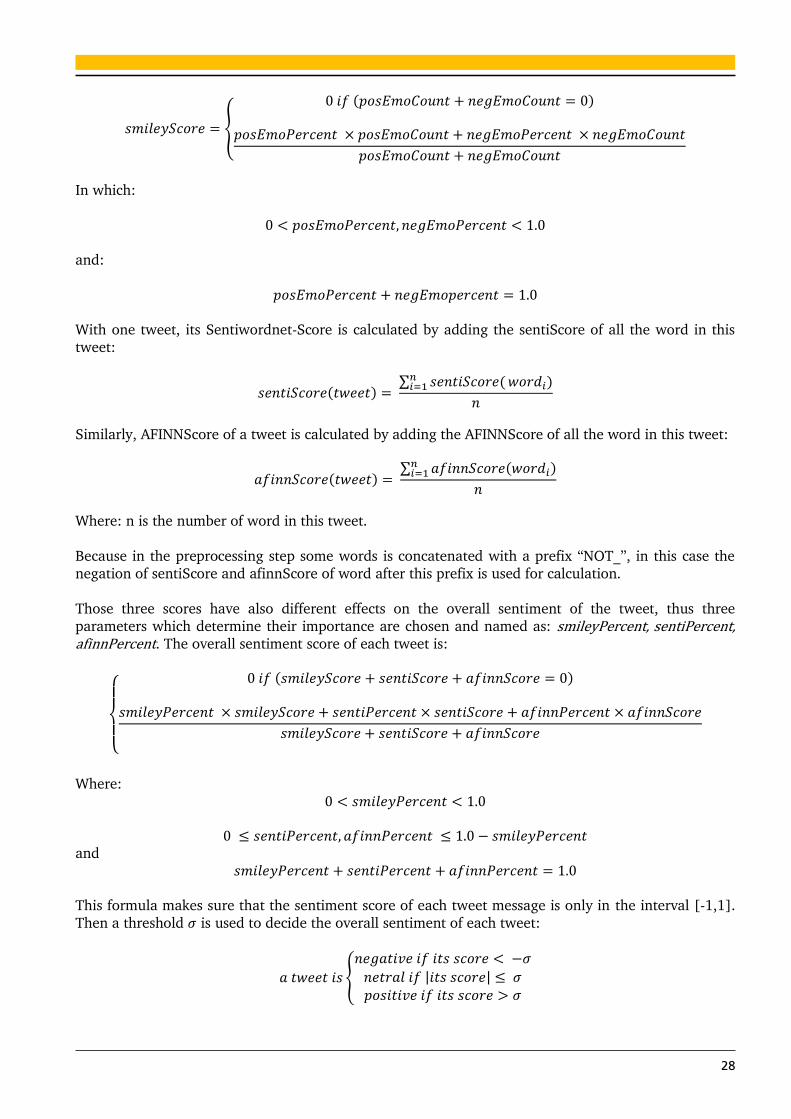
Based on the manual emoticon library which is described in Section 4.2.3, the number of smiley with

positive and negative meaning in a tweet message is calculated as posEmoCount and negEmoCount respectively. Because the negative smileys and positive smiley have the different effects on a tweet,

two parameters are chosen to determine their effects rate. They are called posEmoPercent and

negEmoPercent. The smiley score for each tweet is calculated as:

28

{

In which:

and:

With one tweet, its Sentiwordnet-Score is calculated by adding the sentiScore of all the word in this

tweet:

∑

Similarly, AFINNScore of a tweet is calculated by adding the AFINNScore of all the word in this tweet:

∑

Where: n is the number of word in this tweet.

Because in the preprocessing step some words is concatenated with a prefix “NOT_”, in this case the

negation of sentiScore and afinnScore of word after this prefix is used for calculation.

Those three scores have also different effects on the overall sentiment of the tweet, thus three

parameters which determine their importance are chosen and named as: smileyPercent, sentiPercent, afinnPercent. The overall sentiment score of each tweet is:

{

Where:

and

This formula makes sure that the sentiment score of each tweet message is only in the interval [-1,1].

Then a threshold is used to decide the overall sentiment of each tweet:

{

| |

29

In this approach, the different values of posEmoPercent, smileyPercent, sentiPercent and are used to

obtain the best result on the SET3_GP and SET4.

30

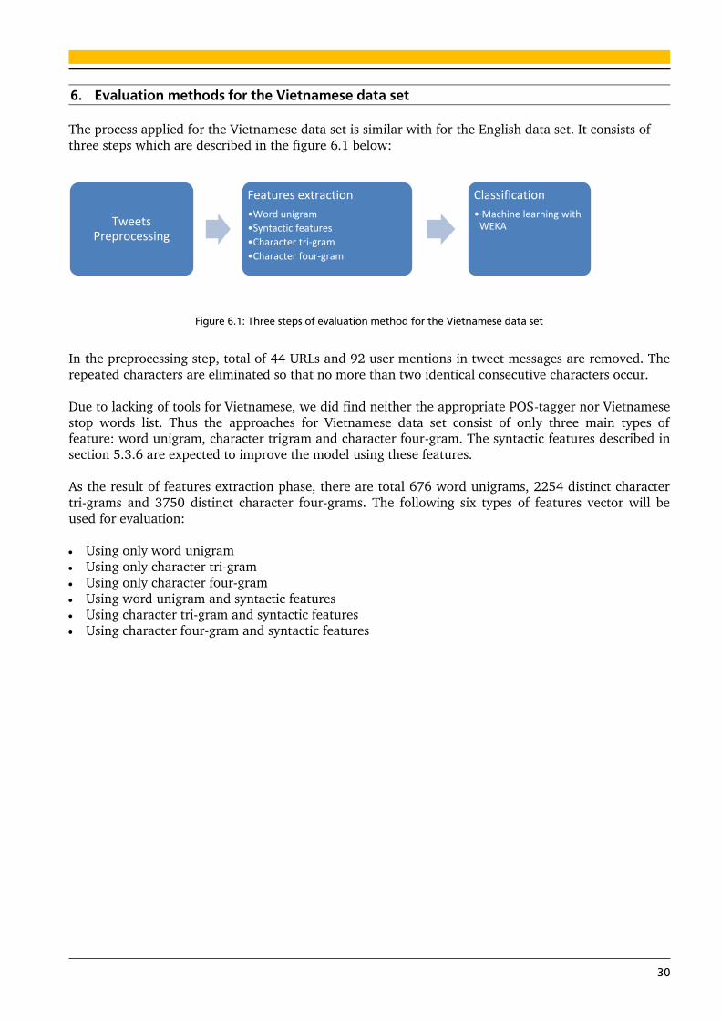
6. Evaluation methods for the Vietnamese data set

The process applied for the Vietnamese data set is similar with for the English data set. It consists of

three steps which are described in the figure 6.1 below:

Figure 6.1: Three steps of evaluation method for the Vietnamese data set

In the preprocessing step, total of 44 URLs and 92 user mentions in tweet messages are removed. The

repeated characters are eliminated so that no more than two identical consecutive characters occur.

Due to lacking of tools for Vietnamese, we did find neither the appropriate POS-tagger nor Vietnamese

stop words list. Thus the approaches for Vietnamese data set consist of only three main types of feature: word unigram, character trigram and character four-gram. The syntactic features described in

section 5.3.6 are expected to improve the model using these features.

As the result of features extraction phase, there are total 676 word unigrams, 2254 distinct character

tri-grams and 3750 distinct character four-grams. The following six types of features vector will be

used for evaluation:

Using only word unigram

Using only character tri-gram

Using only character four-gram

Using word unigram and syntactic features Using character tri-gram and syntactic features

Using character four-gram and syntactic features

Tweets Preprocessing

Features extraction

•Word unigram

•Syntactic features

•Character tri-gram

•Character four-gram

Classification

• Machine learning with WEKA

31

7. Evaluation results

In this chapter, utilization of four above mentioned algorithms (Naïve Bayes Binary Model, Naïve

Bayes Multinomial Model, Support Vector Machine, and Simple Classifier) with different combinations

of features is evaluated. The result - accuracy of each method -, some extensive error analysis including

feature assessment will be summarized in two parts: for English and for Vietnamese. The accuracy is

calculated using stratified 10-fold cross validation.

Stratified K-cross validation is a method to estimate the accuracy of a classifier on one data set. This

data set is divided into K subsets, with size of each subset are approximately equal. The classifier is

then trained using K-1 subsets, and the rest subset is used as a test set. The cross validation runs K

times and the accuracy is calculated by the number of times that the instances are assigned the correct label divided by the number of instances. The stratified K-cross validation ensures that, the instances in

each fold are distributed approximately as same as in the full data set (Kohavi, 1995).

7.1. Evaluation results on the English data sets

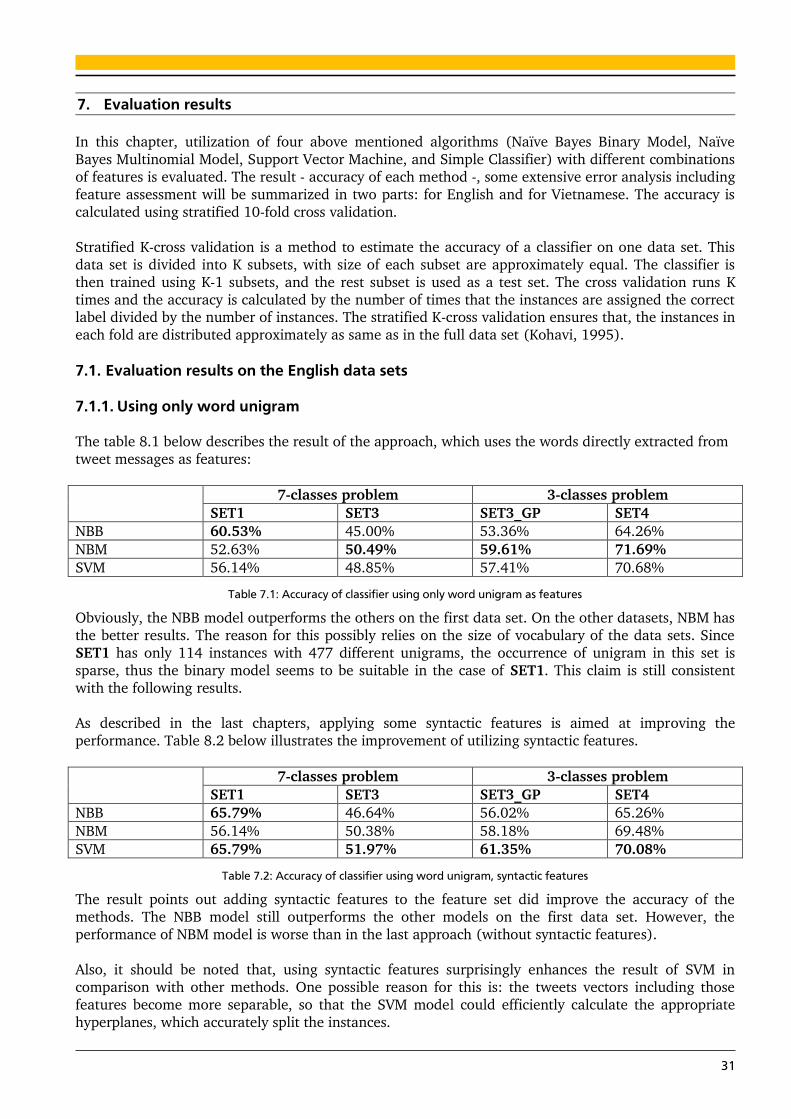
7.1.1. Using only word unigram

The table 8.1 below describes the result of the approach, which uses the words directly extracted from

tweet messages as features:

7-classes problem 3-classes problem

SET1 SET3 SET3_GP SET4

NBB 60.53% 45.00% 53.36% 64.26%

NBM 52.63% 50.49% 59.61% 71.69%

SVM 56.14% 48.85% 57.41% 70.68%

Table 7.1: Accuracy of classifier using only word unigram as features

Obviously, the NBB model outperforms the others on the first data set. On the other datasets, NBM has

the better results. The reason for this possibly relies on the size of vocabulary of the data sets. Since

SET1 has only 114 instances with 477 different unigrams, the occurrence of unigram in this set is

sparse, thus the binary model seems to be suitable in the case of SET1. This claim is still consistent

with the following results.

As described in the last chapters, applying some syntactic features is aimed at improving the

performance. Table 8.2 below illustrates the improvement of utilizing syntactic features.

7-classes problem 3-classes problem

SET1 SET3 SET3_GP SET4

NBB 65.79% 46.64% 56.02% 65.26%

NBM 56.14% 50.38% 58.18% 69.48%

SVM 65.79% 51.97% 61.35% 70.08%

Table 7.2: Accuracy of classifier using word unigram, syntactic features

The result points out adding syntactic features to the feature set did improve the accuracy of the

methods. The NBB model still outperforms the other models on the first data set. However, the

performance of NBM model is worse than in the last approach (without syntactic features).

Also, it should be noted that, using syntactic features surprisingly enhances the result of SVM in

comparison with other methods. One possible reason for this is: the tweets vectors including those

features become more separable, so that the SVM model could efficiently calculate the appropriate

hyperplanes, which accurately split the instances.

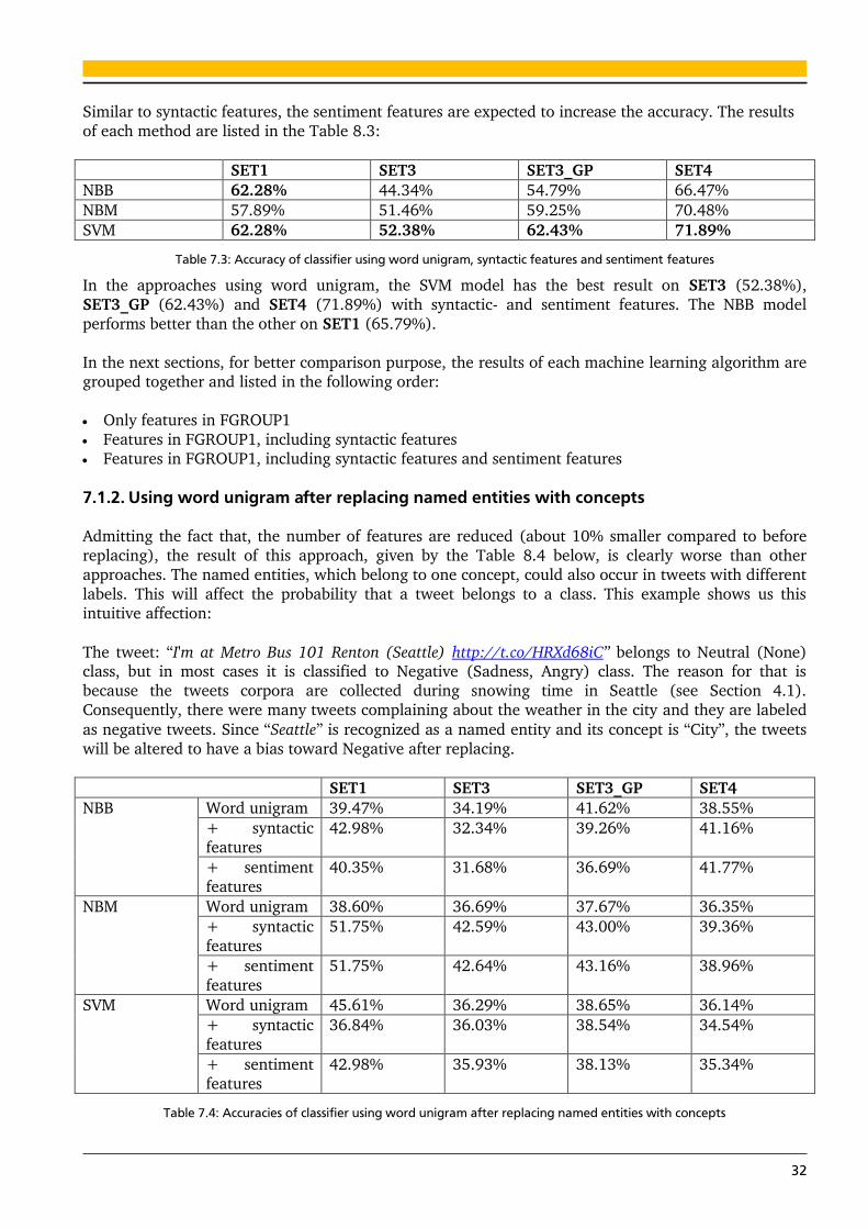
32

Similar to syntactic features, the sentiment features are expected to increase the accuracy. The results

of each method are listed in the Table 8.3:

SET1 SET3 SET3_GP SET4

NBB 62.28% 44.34% 54.79% 66.47%

NBM 57.89% 51.46% 59.25% 70.48%

SVM 62.28% 52.38% 62.43% 71.89%

Table 7.3: Accuracy of classifier using word unigram, syntactic features and sentiment features

In the approaches using word unigram, the SVM model has the best result on SET3 (52.38%),

SET3_GP (62.43%) and SET4 (71.89%) with syntactic- and sentiment features. The NBB model

performs better than the other on SET1 (65.79%).

In the next sections, for better comparison purpose, the results of each machine learning algorithm are

grouped together and listed in the following order:

Only features in FGROUP1

Features in FGROUP1, including syntactic features

Features in FGROUP1, including syntactic features and sentiment features

7.1.2. Using word unigram after replacing named entities with concepts Admitting the fact that, the number of features are reduced (about 10% smaller compared to before

replacing), the result of this approach, given by the Table 8.4 below, is clearly worse than other

approaches. The named entities, which belong to one concept, could also occur in tweets with different

labels. This will affect the probability that a tweet belongs to a class. This example shows us this

intuitive affection:

The tweet: “I'm at Metro Bus 101 Renton (Seattle) http://t.co/HRXd68iC” belongs to Neutral (None) class, but in most cases it is classified to Negative (Sadness, Angry) class. The reason for that is

because the tweets corpora are collected during snowing time in Seattle (see Section 4.1).

Consequently, there were many tweets complaining about the weather in the city and they are labeled

as negative tweets. Since “Seattle” is recognized as a named entity and its concept is “City”, the tweets

will be altered to have a bias toward Negative after replacing.

SET1 SET3 SET3_GP SET4

NBB Word unigram 39.47% 34.19% 41.62% 38.55%

+ syntactic

features

42.98% 32.34% 39.26% 41.16%

+ sentiment

features

40.35% 31.68% 36.69% 41.77%

NBM Word unigram 38.60% 36.69% 37.67% 36.35%

+ syntactic

features

51.75% 42.59% 43.00% 39.36%

+ sentiment

features

51.75% 42.64% 43.16% 38.96%

SVM Word unigram 45.61% 36.29% 38.65% 36.14%

+ syntactic

features

36.84% 36.03% 38.54% 34.54%

+ sentiment

features

42.98% 35.93% 38.13% 35.34%

Table 7.4: Accuracies of classifier using word unigram after replacing named entities with concepts

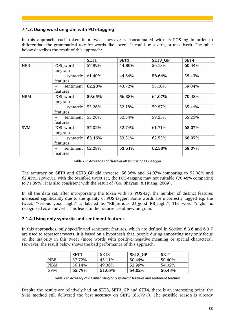
33

7.1.3. Using word unigram with POS-tagging

In this approach, each token in a tweet message is concatenated with its POS-tag in order to

differentiate the grammatical role for words like “over”. It could be a verb, or an adverb. The table

below describes the result of this approach:

SET1 SET3 SET3_GP SET4

NBB POS_word

unigram

57.89% 44.80% 56.18% 60.44%

+ syntactic

features

61.40% 44.64% 56.64% 58.43%

+ sentiment

features

62.28% 43.72% 55.10% 59.04%

NBM POS_word

unigram

59.65% 56.38% 64.07% 70.48%

+ syntactic

features

55.26% 52.18% 59.87% 65.46%

+ sentiment

features

55.26% 52.54% 59.25% 65.26%

SVM POS_word

unigram

57.02% 52.74% 61.71% 68.07%

+ syntactic

features

63.16% 53.31% 62.53% 68.07%

+ sentiment

features

62.28% 53.51% 62.58% 68.07%

Table 7.5: Accuracies of classifier after utilizing POS-tagger

The accuracy on SET3 and SET3_GP did increase: 56.38% and 64.07% comparing to 52.38% and

62.43%. However, with the Stanford tweet set, the POS-tagging may not suitable (70.48% comparing

to 71.89%). It is also consistent with the result of (Go, Bhayani, & Huang, 2009).

In all the data set, after incorporating the token with its POS-tag, the number of distinct features

increased significantly due to the quality of POS-tagger. Some words are incorrectly tagged e.g. the

tweet: “serious good night” is labeled as “RB_serious JJ_good RB_night”. The word “night” is

recognized as an adverb. This leads to the occurrence of new unigram.

7.1.4. Using only syntactic and sentiment features In this approaches, only specific and sentiment features, which are defined in Section 6.3.6 and 6.3.7

are used to represent tweets. It is based on a hypothesis that, people during annotating may only focus

on the majority in this tweet (more words with positive/negative meaning or special characters).

However, the result below shows the bad performance of this approach.

SET1 SET3 SET3_GP SET4

NBB 37.72% 45.11% 50.44% 50.40%

NBM 56.14% 49.36% 52.99% 54.02%

SVM 65.79% 51.05% 54.02% 56.43%

Table 7.6: Accuracy of classifier using only syntactic features and sentiment features

Despite the results are relatively bad on SET3, SET3_GP and SET4, there is an interesting point: the

SVM method still delivered the best accuracy on SET1 (65.79%). The possible reason is already

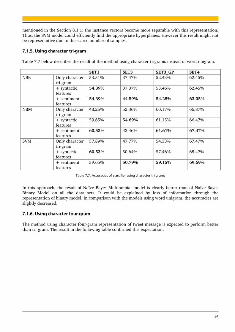
34

mentioned in the Section 8.1.1: the instance vectors become more separable with this representation.

Thus, the SVM model could efficiently find the appropriate hyperplanes. However this result might not

be representative due to the scarce number of samples.

7.1.5. Using character tri-gram

Table 7.7 below describes the result of the method using character-trigrams instead of word unigram.

SET1 SET3 SET3_GP SET4

NBB Only character

tri-gram

53.51% 37.47% 52.43% 62.45%

+ syntactic

features

54.39% 37.37% 53.46% 62.45%

+ sentiment

features

54.39% 44.59% 54.28% 63.05%

NBM Only character

tri-gram

48.25% 53.36% 60.17% 66.87%

+ syntactic

features

59.65% 54.69% 61.15% 66.47%

+ sentiment

features

60.53% 43.46% 61.61% 67.47%

SVM Only character

tri-gram

57.89% 47.77% 54.33% 67.47%

+ syntactic

features

60.53% 50.64% 57.46% 68.47%

+ sentiment

features

59.65% 50.79% 59.15% 69.69%

Table 7.7: Accuracies of classifier using character tri-grams

In this approach, the result of Naïve Bayes Multinomial model is clearly better than of Naïve Bayes

Binary Model on all the data sets. It could be explained by loss of information through the representation of binary model. In comparison with the models using word unigram, the accuracies are

slightly decreased.

7.1.6. Using character four-gram

The method using character four-gram representation of tweet message is expected to perform better

than tri-gram. The result in the following table confirmed this expectation:

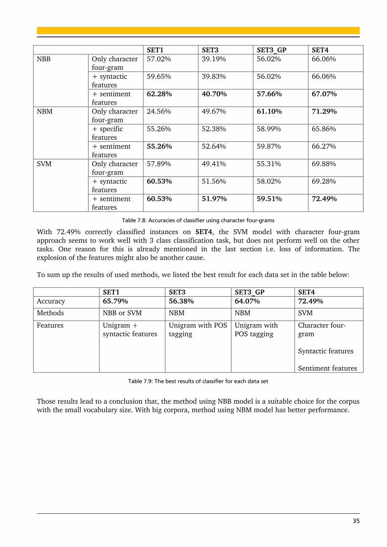
35

SET1 SET3 SET3_GP SET4

NBB Only character

four-gram

57.02% 39.19% 56.02% 66.06%

+ syntactic

features

59.65% 39.83% 56.02% 66.06%

+ sentiment

features

62.28% 40.70% 57.66% 67.07%

NBM Only character

four-gram

24.56% 49.67% 61.10% 71.29%

+ specific

features

55.26% 52.38% 58.99% 65.86%

+ sentiment

features

55.26% 52.64% 59.87% 66.27%

SVM Only character

four-gram

57.89% 49.41% 55.31% 69.88%

+ syntactic

features

60.53% 51.56% 58.02% 69.28%

+ sentiment

features

60.53% 51.97% 59.51% 72.49%

Table 7.8: Accuracies of classifier using character four-grams

With 72.49% correctly classified instances on SET4, the SVM model with character four-gram

approach seems to work well with 3 class classification task, but does not perform well on the other

tasks. One reason for this is already mentioned in the last section i.e. loss of information. The

explosion of the features might also be another cause.

To sum up the results of used methods, we listed the best result for each data set in the table below:

SET1 SET3 SET3_GP SET4

Accuracy 65.79% 56.38% 64.07% 72.49%

Methods NBB or SVM NBM NBM SVM

Features Unigram +

syntactic features Unigram with POS

tagging Unigram with

POS tagging Character four-

gram

Syntactic features

Sentiment features

Table 7.9: The best results of classifier for each data set

Those results lead to a conclusion that, the method using NBB model is a suitable choice for the corpus

with the small vocabulary size. With big corpora, method using NBM model has better performance.

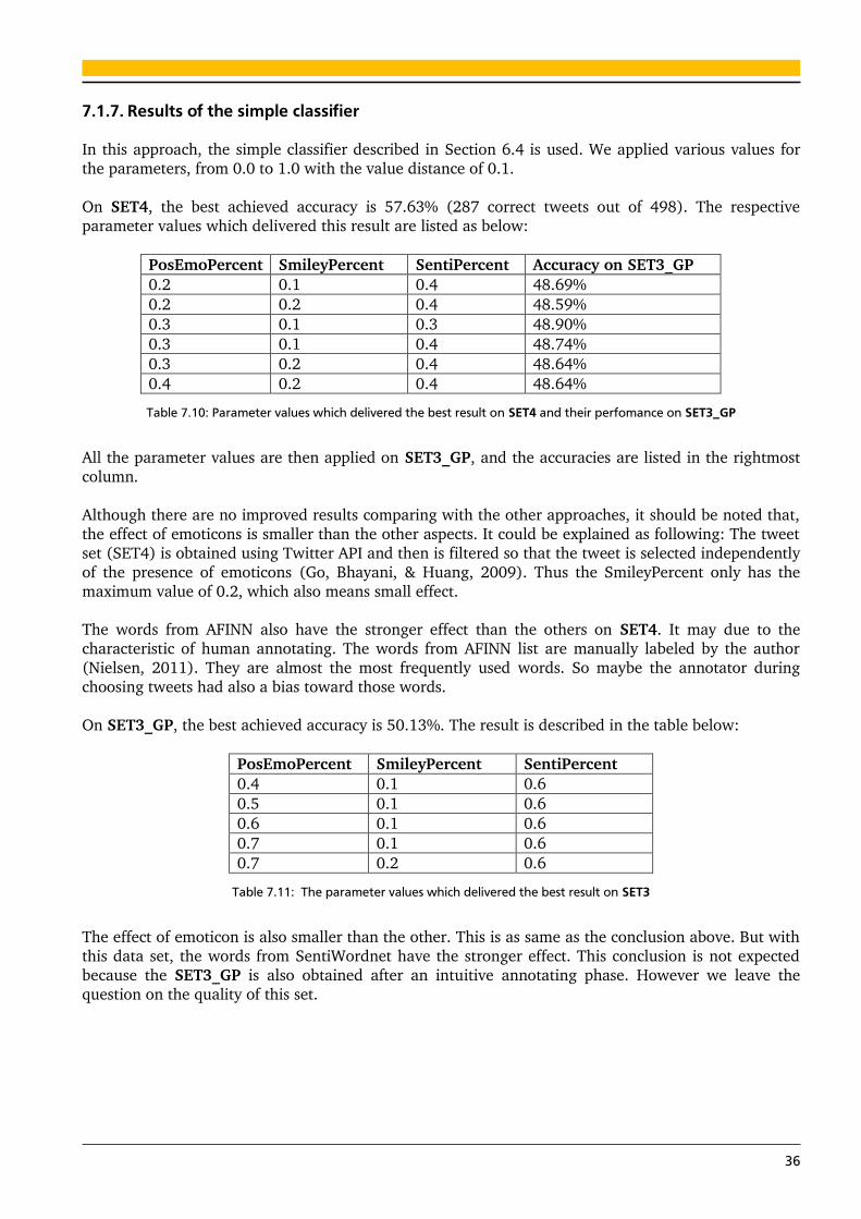
36

7.1.7. Results of the simple classifier

In this approach, the simple classifier described in Section 6.4 is used. We applied various values for

the parameters, from 0.0 to 1.0 with the value distance of 0.1.

On SET4, the best achieved accuracy is 57.63% (287 correct tweets out of 498). The respective

parameter values which delivered this result are listed as below:

PosEmoPercent SmileyPercent SentiPercent Accuracy on SET3_GP

0.2 0.1 0.4 48.69%

0.2 0.2 0.4 48.59%

0.3 0.1 0.3 48.90%

0.3 0.1 0.4 48.74%

0.3 0.2 0.4 48.64%

0.4 0.2 0.4 48.64%

Table 7.10: Parameter values which delivered the best result on SET4 and their perfomance on SET3_GP

All the parameter values are then applied on SET3_GP, and the accuracies are listed in the rightmost

column.

Although there are no improved results comparing with the other approaches, it should be noted that,

the effect of emoticons is smaller than the other aspects. It could be explained as following: The tweet

set (SET4) is obtained using Twitter API and then is filtered so that the tweet is selected independently

of the presence of emoticons (Go, Bhayani, & Huang, 2009). Thus the SmileyPercent only has the

maximum value of 0.2, which also means small effect.

The words from AFINN also have the stronger effect than the others on SET4. It may due to the

characteristic of human annotating. The words from AFINN list are manually labeled by the author

(Nielsen, 2011). They are almost the most frequently used words. So maybe the annotator during

choosing tweets had also a bias toward those words.

On SET3_GP, the best achieved accuracy is 50.13%. The result is described in the table below:

PosEmoPercent SmileyPercent SentiPercent

0.4 0.1 0.6

0.5 0.1 0.6

0.6 0.1 0.6

0.7 0.1 0.6

0.7 0.2 0.6

Table 7.11: The parameter values which delivered the best result on SET3

The effect of emoticon is also smaller than the other. This is as same as the conclusion above. But with

this data set, the words from SentiWordnet have the stronger effect. This conclusion is not expected

because the SET3_GP is also obtained after an intuitive annotating phase. However we leave the

question on the quality of this set.

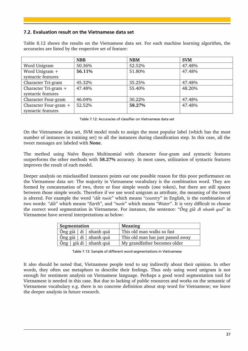
37

7.2. Evaluation result on the Vietnamese data set

Table 8.12 shows the results on the Vietnamese data set. For each machine learning algorithm, the

accuracies are listed by the respective set of feature:

NBB NBM SVM

Word Unigram 50.36% 52.52% 47.48%

Word Unigram +

syntactic features

56.11% 51.80% 47.48%

Character Tri-gram 45.32% 35.25% 47.48%

Character Tri-gram + syntactic features

47.48% 55.40% 48.20%

Character Four-gram 46.04% 30.22% 47.48%

Character Four-gram + syntactic features

52.52% 58.27% 47.48%

Table 7.12: Accuracies of classifier on Vietnamese data set

On the Vietnamese data set, SVM model tends to assign the most popular label (which has the most

number of instances in training set) to all the instances during classification step. In this case, all the

tweet messages are labeled with None.

The method using Naïve Bayes Multinomial with character four-gram and syntactic features

outperforms the other methods with 58.27% accuracy. In most cases, utilization of syntactic features

improves the result of each model.

Deeper analysis on misclassified instances points out one possible reason for this poor performance on

the Vietnamese data set: The majority in Vietnamese vocabulary is the combination word. They are

formed by concatenation of two, three or four simple words (one token), but there are still spaces between those simple words. Therefore if we use word unigram as attribute, the meaning of the tweet

is altered. For example the word “đất nước” which means “country” in English, is the combination of

two words: “đất” which means “Earth”, and “nước” which means “Water”. It is very difficult to choose

the correct word segmentation in Vietnamese. For instance, the sentence: “Ông già đi nhanh quá” in

Vietnamese have several interpretations as below:

Segmentation Meaning

Ông già | đi | nhanh quá This old man walks so fast

Ông già | đi | nhanh quá This old man has just passed away

Ông | già đi | nhanh quá My grandfather becomes older

Table 7.13: Sample of different word segmentations in Vietnamese

It also should be noted that, Vietnamese people tend to say indirectly about their opinion. In other

words, they often use metaphors to describe their feelings. Thus only using word unigram is not

enough for sentiment analysis on Vietnamese language. Perhaps a good word segmentation tool for

Vietnamese is needed in this case. But due to lacking of public resources and works on the semantic of

Vietnamese vocabulary e.g. there is no concrete definition about stop word for Vietnamese; we leave the deeper analysis in future research.

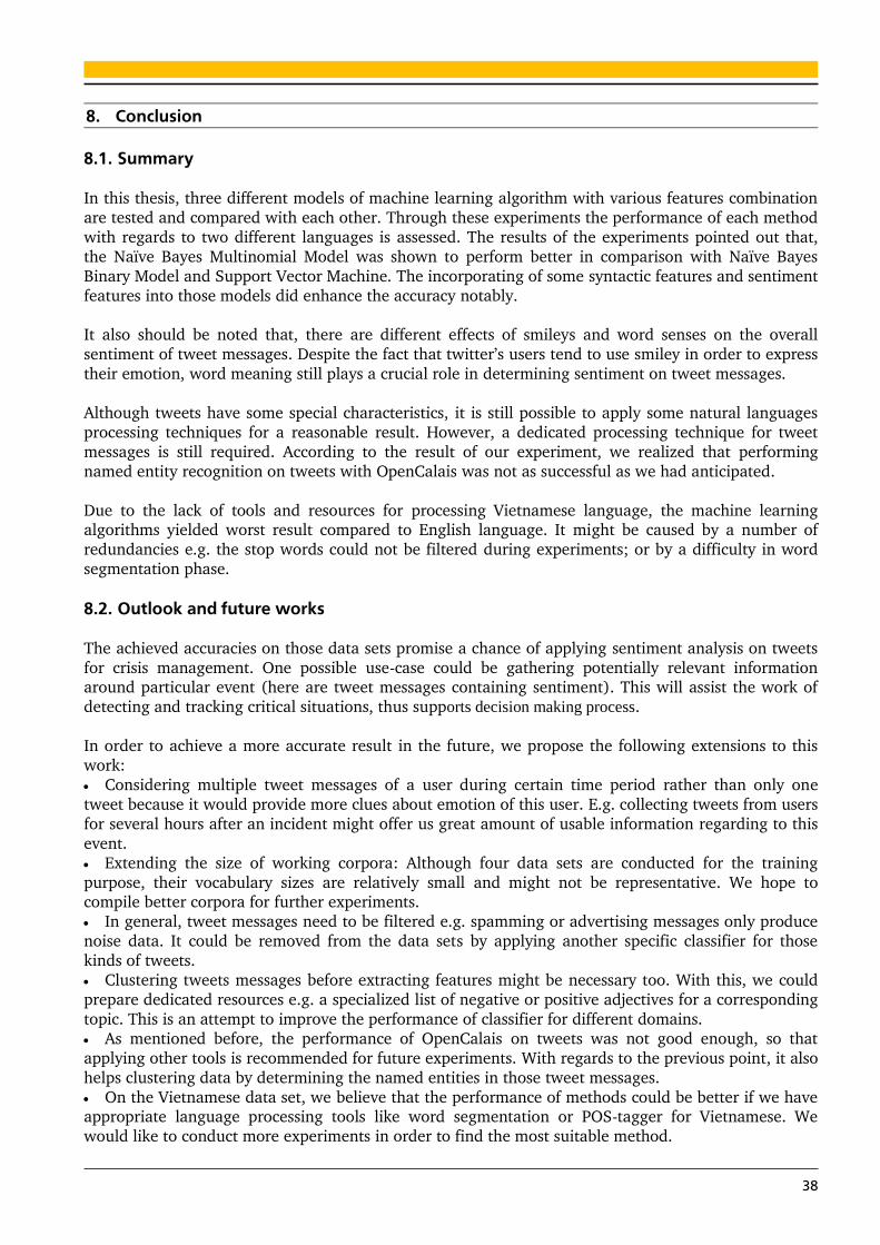
38

8. Conclusion

8.1. Summary

In this thesis, three different models of machine learning algorithm with various features combination

are tested and compared with each other. Through these experiments the performance of each method

with regards to two different languages is assessed. The results of the experiments pointed out that,

the Naïve Bayes Multinomial Model was shown to perform better in comparison with Naïve Bayes

Binary Model and Support Vector Machine. The incorporating of some syntactic features and sentiment

features into those models did enhance the accuracy notably.

It also should be noted that, there are different effects of smileys and word senses on the overall

sentiment of tweet messages. Despite the fact that twitter’s users tend to use smiley in order to express

their emotion, word meaning still plays a crucial role in determining sentiment on tweet messages.

Although tweets have some special characteristics, it is still possible to apply some natural languages

processing techniques for a reasonable result. However, a dedicated processing technique for tweet

messages is still required. According to the result of our experiment, we realized that performing

named entity recognition on tweets with OpenCalais was not as successful as we had anticipated.

Due to the lack of tools and resources for processing Vietnamese language, the machine learning algorithms yielded worst result compared to English language. It might be caused by a number of

redundancies e.g. the stop words could not be filtered during experiments; or by a difficulty in word

segmentation phase.

8.2. Outlook and future works

The achieved accuracies on those data sets promise a chance of applying sentiment analysis on tweets

for crisis management. One possible use-case could be gathering potentially relevant information around particular event (here are tweet messages containing sentiment). This will assist the work of

detecting and tracking critical situations, thus supports decision making process.

In order to achieve a more accurate result in the future, we propose the following extensions to this

work:

Considering multiple tweet messages of a user during certain time period rather than only one

tweet because it would provide more clues about emotion of this user. E.g. collecting tweets from users

for several hours after an incident might offer us great amount of usable information regarding to this

event.

Extending the size of working corpora: Although four data sets are conducted for the training

purpose, their vocabulary sizes are relatively small and might not be representative. We hope to compile better corpora for further experiments.

In general, tweet messages need to be filtered e.g. spamming or advertising messages only produce

noise data. It could be removed from the data sets by applying another specific classifier for those

kinds of tweets.

Clustering tweets messages before extracting features might be necessary too. With this, we could

prepare dedicated resources e.g. a specialized list of negative or positive adjectives for a corresponding

topic. This is an attempt to improve the performance of classifier for different domains.

As mentioned before, the performance of OpenCalais on tweets was not good enough, so that

applying other tools is recommended for future experiments. With regards to the previous point, it also

helps clustering data by determining the named entities in those tweet messages.

On the Vietnamese data set, we believe that the performance of methods could be better if we have appropriate language processing tools like word segmentation or POS-tagger for Vietnamese. We

would like to conduct more experiments in order to find the most suitable method.

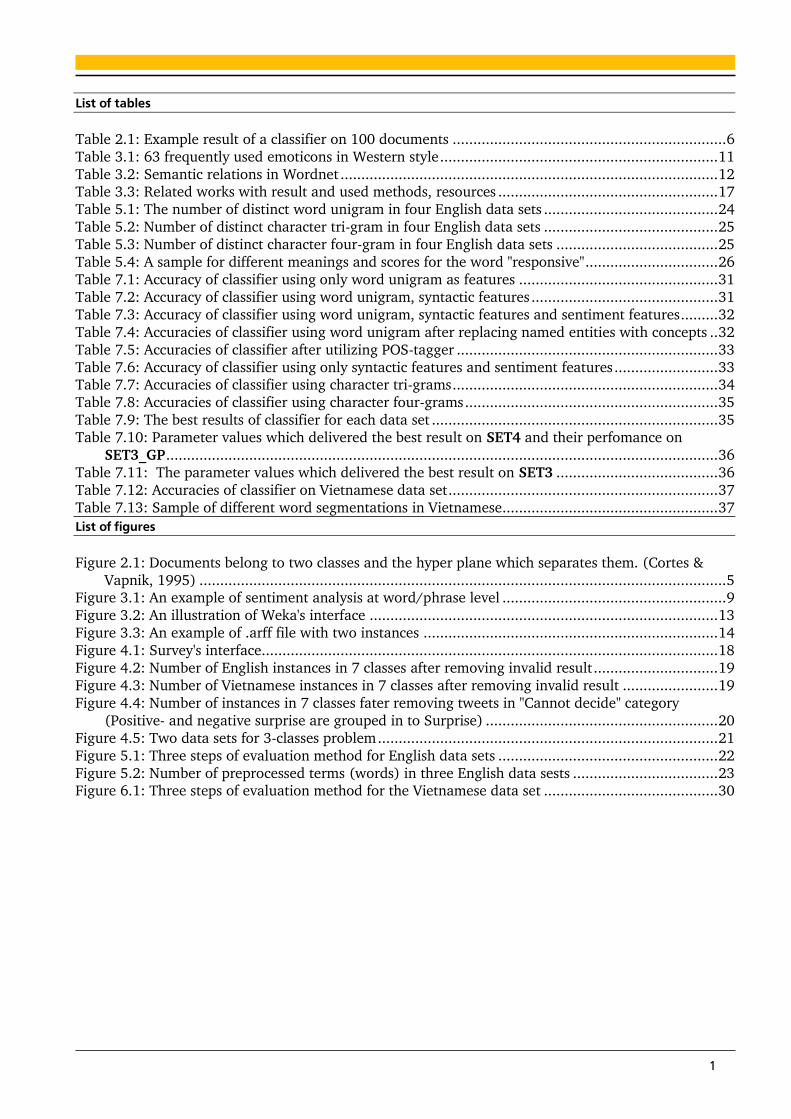
1

List of tables

Table 2.1: Example result of a classifier on 100 documents .................................................................. 6 Table 3.1: 63 frequently used emoticons in Western style ................................................................... 11 Table 3.2: Semantic relations in Wordnet ........................................................................................... 12 Table 3.3: Related works with result and used methods, resources ..................................................... 17 Table 5.1: The number of distinct word unigram in four English data sets .......................................... 24 Table 5.2: Number of distinct character tri-gram in four English data sets .......................................... 25 Table 5.3: Number of distinct character four-gram in four English data sets ....................................... 25 Table 5.4: A sample for different meanings and scores for the word "responsive" ................................ 26 Table 7.1: Accuracy of classifier using only word unigram as features ................................................ 31 Table 7.2: Accuracy of classifier using word unigram, syntactic features ............................................. 31 Table 7.3: Accuracy of classifier using word unigram, syntactic features and sentiment features ......... 32 Table 7.4: Accuracies of classifier using word unigram after replacing named entities with concepts .. 32 Table 7.5: Accuracies of classifier after utilizing POS-tagger ............................................................... 33 Table 7.6: Accuracy of classifier using only syntactic features and sentiment features ......................... 33 Table 7.7: Accuracies of classifier using character tri-grams ................................................................ 34 Table 7.8: Accuracies of classifier using character four-grams ............................................................. 35 Table 7.9: The best results of classifier for each data set ..................................................................... 35 Table 7.10: Parameter values which delivered the best result on SET4 and their perfomance on

SET3_GP ..................................................................................................................................... 36 Table 7.11: The parameter values which delivered the best result on SET3 ....................................... 36 Table 7.12: Accuracies of classifier on Vietnamese data set ................................................................. 37 Table 7.13: Sample of different word segmentations in Vietnamese .................................................... 37

List of figures

Figure 2.1: Documents belong to two classes and the hyper plane which separates them. (Cortes &

Vapnik, 1995) ............................................................................................................................... 5 Figure 3.1: An example of sentiment analysis at word/phrase level ...................................................... 9 Figure 3.2: An illustration of Weka's interface .................................................................................... 13 Figure 3.3: An example of .arff file with two instances ....................................................................... 14 Figure 4.1: Survey's interface .............................................................................................................. 18 Figure 4.2: Number of English instances in 7 classes after removing invalid result .............................. 19 Figure 4.3: Number of Vietnamese instances in 7 classes after removing invalid result ....................... 19 Figure 4.4: Number of instances in 7 classes fater removing tweets in "Cannot decide" category

(Positive- and negative surprise are grouped in to Surprise) ........................................................ 20 Figure 4.5: Two data sets for 3-classes problem .................................................................................. 21 Figure 5.1: Three steps of evaluation method for English data sets ..................................................... 22 Figure 5.2: Number of preprocessed terms (words) in three English data sests ................................... 23 Figure 6.1: Three steps of evaluation method for the Vietnamese data set .......................................... 30

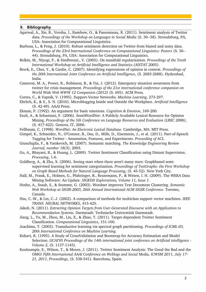
2

9. Bibliography

Agarwal, A., Xie, B., Vovsha, I., Rambow, O., & Passonneau, R. (2011). Sentiment analysis of Twitter

data. Proceedings of the Workshop on Languages in Social Media (S. 30--38). Stroudsburg, PA,

USA: Association for Computational Linguistics.

Barbosa, L., & Feng, J. (2010). Robust sentiment detection on Twitter from biased and noisy data.

Proceedings of the 23rd International Conference on Computational Linguistics: Posters (S. 36--44). Stroudsburg, PA, USA: Association for Computational Linguistics.

Belkin, M., Niyogi, P., & Sindhwani., V. (2005). On manifold regularization. Proceedings of the Tenth

International Workshop on Artificial Intelligence and Statistics (AISTAT 2005).

Breck, E., Choi, Y., & Cardie, C. (2007). Identifying expressions of opinion in context. Proceedings of

the 20th International Joint Conference on Artificial Intelligence, (S. 2683-2688). Hyderabad,

India.

Cameron, M. A., Power, R., Robinson, B., & Yin, J. (2012). Emergency situation awareness from

twitter for crisis management. Proceedings of the 21st international conference companion on

World Wide Web WWW 12 Companion (2012) (S. 695). ACM Press.

Cortes, C., & Vapnik, V. (1995). Support-Vector Networks. Machine Learning, 273-297.

Ehrlich, K., & S., S. N. (2010). Microblogging Inside and Outside the Workplace. Artificial Intelligence

(S. 42-49). AAAI Press.

Ekman, P. (1992). An argument for basic emotions. Cognition & Emotion, 169-200. Esuli, A., & Sebastiani, F. (2006). SentiWordNet: A Publicly Available Lexical Resource for Opinion

Mining. Proceedings of the 5th Conference on Language Resources and Evaluation (LREC 2006), (S. 417-422). Genova, IT, 2006.

Fellbaum, C. (1998). WordNet: An Electronic Lexical Database. Cambridge, MA: MIT Press.

Gimpel, K., Schneider, N., O’Connor, B., Das, D., Mills, D., Eisenstein, J., et al. (2011). Part-of-Speech

Tagging for Twitter : Annotation, Features, and Experiments. Proceeding of ACL.

Giunchiglia, F., & Yatskevich, M. (2007). Semantic matching. The Knowledge Engineering Review

Journal, number 18(3), 2003. Go, A., Bhayani, R., & Huang, L. (2009). Twitter Sentiment Classification using Distant Supervision.

Processing, 1-6. Goldberg, A., & Zhu, X. (2006). Seeing stars when there aren’t many stars: Graphbased semi-

supervised learning for sentiment categorization. Proceedings of TextGraphs: the First Workshop

on Graph Based Methods for Natural Language Processing, (S. 45-52). New York City. Hall, M., Frank, E., Holmes, G., Pfahringer, B., Reutemann, P., & Witten, I. H. (2009). The WEKA Data

Mining Software: An Update. SIGKDD Explorations, Volume 11, Issue 1.

Hotho, A., Staab, S., & Stumme, G. (2003). Wordnet improves Text Document Clustering. Semantic

Web Workshop at SIGIR-2003, 26th Annual International ACM SIGIR Conference. Toronto,

Canada.

Hsu, C.-W., & Lin, C.-J. (2002). A comparison of methods for multiclass support vector machines. IEEE

TRANS. NEURAL NETWORKS, 415-425.

Jakob, N. (2011). Extracting Opinion Targets from User-Generated Discourse with an Application to

Recommendation Systems. Darmstadt: Technische Universtität Darmstadt. Jiang, L., Yu, M., Zhou, M., Liu, X., & Zhao, T. (2011). Target-dependent Twitter Sentiment

Classification. Computational Linguistics, 151-160.

Joachims, T. (2003). Transductive learning via spectral graph partitioning. Proceedings of ICML-03,

20th International Conference on Machine Learning.

Kohavi, R. (1995). A Study of CrossValidation and Bootstrap for Accuracy Estimation and Model

Selection. IJCAI'95 Proceedings of the 14th international joint conference on Artificial intelligence -

Volume 2, (S. 1137-1143). Kouloumpis, E., Wilson, T., & Moore, J. (2011). Twitter Sentiment Analysis: The Good the Bad and the

OMG! Fifth International AAAI Conference on Weblogs and Social Media, ICWSM 2011, July 17-

21, 2011, Proceedings, (S. 538-541). Barcelona, Spain.

3

Lafferty, J., McCallum, A., & Pereira, F. (2001). Conditional Random Fields: Probabilistic Models for

Segmenting and Labeling Sequence Data. (S. 282-289). Morgan Kaufmann.

Marcus, M. P., Santorini, B., & Ann, M. (1993). Building a large annotated corpus of English: The Penn

Treebank. Computational Linguistics, 19:313-330. McDonald, R., Hannan, K., Neylon, T., Wells, M., & Reynar, J. (2007). Structured models for fine-to-

coarse sentiment analysis. Proceedings of the 45th Annual Meeting of the Association of

Computational Linguistics, (S. 432-439). Prague, Czech Republic.

Miller, G. A. (1995). WordNet: A Lexical Database for English. Communications of the ACM Vol. 38, No.

11, 39-41.

Nagy, A., & Stammberger, J. (2012). Crowd Sentiment Detection during Disasters and Crises.

Proceedings of the 9th International ISCRAM Conference, (S. 1-9). Vancouver, Canada.

Nielsen, A. (2011). A new ANEW : Evaluation of a word list for sentiment analysis in microblogs. Word

Journal Of The International Linguistic Association, 93-98. Pang, B., & Lee, L. (2004). A sentimental education: Sentiment analysis using subjectivity

summarization based on minimum cuts. Proceedings of ACL, (S. 271-278). Pang, B., & Lee, L. (2005). Seeing stars: Exploiting class relationships for sentiment categorization

with respect to rating scales. Proceedings of the 43rd Annual Meeting of the Association for

Computational Linguistics, (S. 115-124). Ann Arbor, Michigan, USA.

Pang, B., & Lee, L. (2006). Opinion Mining and Sentiment Analysis. Foundations and Trends® in

Information Retrieval, 91-231. Pang, B., Lee, L., & Vaithyanathan, S. (2002). Thumbs up? sentiment classification using machine

learning techniques. 7th Conference on Empirical Methods in Natural Language Processing, (S.

79-86). Philadelphia, Pennsylvania, USA.

Saif, H., He, Y., & Alani, H. (2012). Alleviating Data Sparsity for Twitter Sentiment Analysis.

Workshop: The 2nd Workshop on Making Sense of Microposts (#MSM2012): Big things come in

small packages at World Wide Web (WWW) 2012. Lyon, France.

Wiebe, J., & Wilson, T. (2002). Learning to disambiguate potentially subjective expressions. 6th

Conference on Natural Language Learning, (S. 112-118). Taipei, Taiwan.

Witten, I. H., & Frank, E. (2005). Data mining: Pratice Machine Learning Tools and Techniques 2nd

Edition. San Francisco: Morgan Kaufmann Publishers.