UNIVERSITÀ DEGLI STUDI DI PADOVA

DIPARTIMENTO DI INGEGNERIA DELL’INFORMAZIONE

Corso di Laurea Magistrale in Ingegneria Informatica

Tesi di Laurea

Evaluation of Microsoft Kinect 360 and Microsoft Kinect One for robotics and

computer vision applications

Student: Simone Zennaro Advisor: Prof. Emanuele Menegatti

Co-Advisor: Dott. Ing. Matteo Munaro

9 Dicembre 2014 Anno Accademico 2014/2015

2

Dedico questa tesi ai miei genitori che in questi duri anni di studio mi

hanno sempre sostenuto e supportato nelle mie decisioni.

3

Gli scienziati sognano di fare grandi cose.

Gli ingegneri le realizzano. James A. Michener

TABLE OF CONTENTS

Abstract ......................................................................................................................................................... 6

1 Introduction .......................................................................................................................................... 7

1.1 Kinect XBOX 360 ............................................................................................................................ 7

1.1.1 Principle of depth measurement by triangulation ................................................................ 7

1.2 Kinect XBOX ONE ........................................................................................................................ 10

1.2.1 Principle of depth measurement by time of flight .............................................................. 13

1.2.2 Driver and SDK .................................................................................................................... 16

1.2.3 Survey of Open Source Drivers and SDKs............................................................................ 22

2 Kinect Recorder ................................................................................................................................... 29

2.1 C++ VS C# .................................................................................................................................... 29

2.2 Optimal solution ......................................................................................................................... 30

2.3 The code ...................................................................................................................................... 32

2.3.1 Initialization ......................................................................................................................... 32

2.3.2 Update ................................................................................................................................. 32

2.3.3 Processing ........................................................................................................................... 33

2.3.4 Encoding RGB image ........................................................................................................... 33

2.3.5 Saving .................................................................................................................................. 34

3 Sensors comparison ............................................................................................................................ 39

3.1.2 Point cloud comparison ...................................................................................................... 43

3.1.3 Results ................................................................................................................................. 46

3.2 Outdoors test .............................................................................................................................. 46

3.2.1 Setup ................................................................................................................................... 46

3.2.2 Wall in shadow .................................................................................................................... 47

3.2.3 Wall in sun ........................................................................................................................... 49

5

3.2.4 Car ....................................................................................................................................... 51

3.2.5 Results ................................................................................................................................. 54

3.3 Far field test ................................................................................................................................ 54

3.3.1 Setup ................................................................................................................................... 54

3.3.2 Results ................................................................................................................................. 56

3.4 Color test ..................................................................................................................................... 59

3.4.1 Setup ................................................................................................................................... 59

3.4.2 Results ................................................................................................................................. 60

4 Applications comparison ..................................................................................................................... 63

4.1 People tracking and following ..................................................................................................... 63

4.1.1 Introduction ........................................................................................................................ 63

4.1.2 Pioneer 3-AT ........................................................................................................................ 64

4.1.3 Setup ................................................................................................................................... 64

4.1.4 Test ...................................................................................................................................... 65

4.1.5 Results ................................................................................................................................. 68

4.2 People Tracking scores ................................................................................................................ 69

4.2.1 Setup ................................................................................................................................... 69

4.2.2 Results ................................................................................................................................. 70

5 Conclusions ......................................................................................................................................... 72

References ................................................................................................................................................ 73

6

ABSTRACT

The Microsoft Kinect was developed to replace the traditional controller and to allow a new interaction

with videogames; the low cost and the camera’s portability have made it immediately popular for many

other purposes. The first Kinect has a RGB camera, a depth sensor, which is composed of an infrared laser

projector and an infrared camera sensitive to the same band, and an array of microphones. Although the

low depth resolution and the high image quantization, that makes impossible to reveal small details, the

Kinect was used in many computer vision application. The new one represents a big step forward, not

only for the higher sensors’ resolution, but also for the new technology being used; it exploits a time of

flight sensor to create the depth image. To understand which one is better in computer vision or robotic

applications, an in-depth study of the two Kinects is necessary. In the first section of this thesis, the Kinects’

features will be compared by some tests; in the second section, instead, these sensors will be evaluated

and compared for the purpose of robotics and computer vision applications.

7

1 INTRODUCTION

1.1 KINECT XBOX 360

The Microsoft Kinect was originally launched in November 2010 as an accessory for the Microsoft Xbox

360 video game console. It was developed by the PrimeSense company in conjunction with Microsoft. The

device was meant to provide a completely new way of interacting with the console by means of gestures

and voice instead of the traditional controller. Researchers quickly saw the great potential this versatile

and affordable device offered.

The Kinect is a RGB-D camera based on structured light and it is composed of a RGB camera, an infrared

camera and an array of microphones.

1.1.1 Principle of depth measurement by triangulation

The [1] explains well how Kinect 360 works. The Kinect sensor consists of an infrared laser emitter, an

infrared camera and an RGB camera. The inventors describe the measurement of depth as a triangulation

process (Freedman et al., 2010). The laser source emits a single beam which is split into multiple beams

by a diffraction grating to create a constant pattern of speckles projected onto the scene. This pattern is

captured by the infrared camera and is correlated against a reference pattern. The reference pattern is

obtained by capturing a plane at a known distance from the sensor, and is stored in the memory of the

sensor. When a speckle is projected on an object whose distance to the sensor is smaller or larger than

that of the reference plane the position of the speckle in the infrared image will be shifted in the direction

of the baseline between the laser projector and the perspective centre of the infrared camera.

8

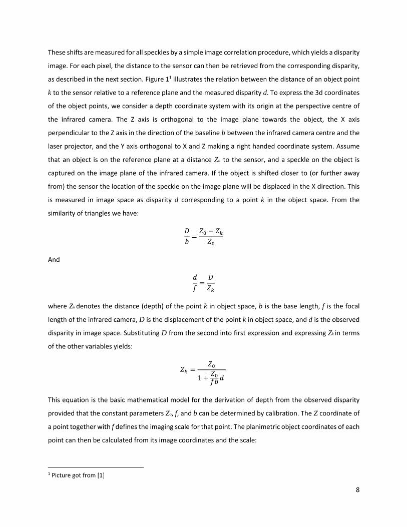
These shifts are measured for all speckles by a simple image correlation procedure, which yields a disparity

image. For each pixel, the distance to the sensor can then be retrieved from the corresponding disparity,

as described in the next section. Figure 11 illustrates the relation between the distance of an object point

k to the sensor relative to a reference plane and the measured disparity d. To express the 3d coordinates

of the object points, we consider a depth coordinate system with its origin at the perspective centre of

the infrared camera. The Z axis is orthogonal to the image plane towards the object, the X axis

perpendicular to the Z axis in the direction of the baseline b between the infrared camera centre and the

laser projector, and the Y axis orthogonal to X and Z making a right handed coordinate system. Assume

that an object is on the reference plane at a distance Zo to the sensor, and a speckle on the object is

captured on the image plane of the infrared camera. If the object is shifted closer to (or further away

from) the sensor the location of the speckle on the image plane will be displaced in the X direction. This

is measured in image space as disparity d corresponding to a point k in the object space. From the

similarity of triangles we have:

𝐷

𝑏=

𝑍0 − 𝑍𝑘

𝑍0

And

𝑑

𝑓=

𝐷

𝑍𝑘

where Zk denotes the distance (depth) of the point k in object space, b is the base length, f is the focal

length of the infrared camera, D is the displacement of the point k in object space, and d is the observed

disparity in image space. Substituting D from the second into first expression and expressing Zk in terms

of the other variables yields:

𝑍𝑘 =𝑍0

1 +𝑍0𝑓𝑏

𝑑

This equation is the basic mathematical model for the derivation of depth from the observed disparity

provided that the constant parameters Zo, f, and b can be determined by calibration. The Z coordinate of

a point together with f defines the imaging scale for that point. The planimetric object coordinates of each

point can then be calculated from its image coordinates and the scale:

1 Picture got from [1]

9

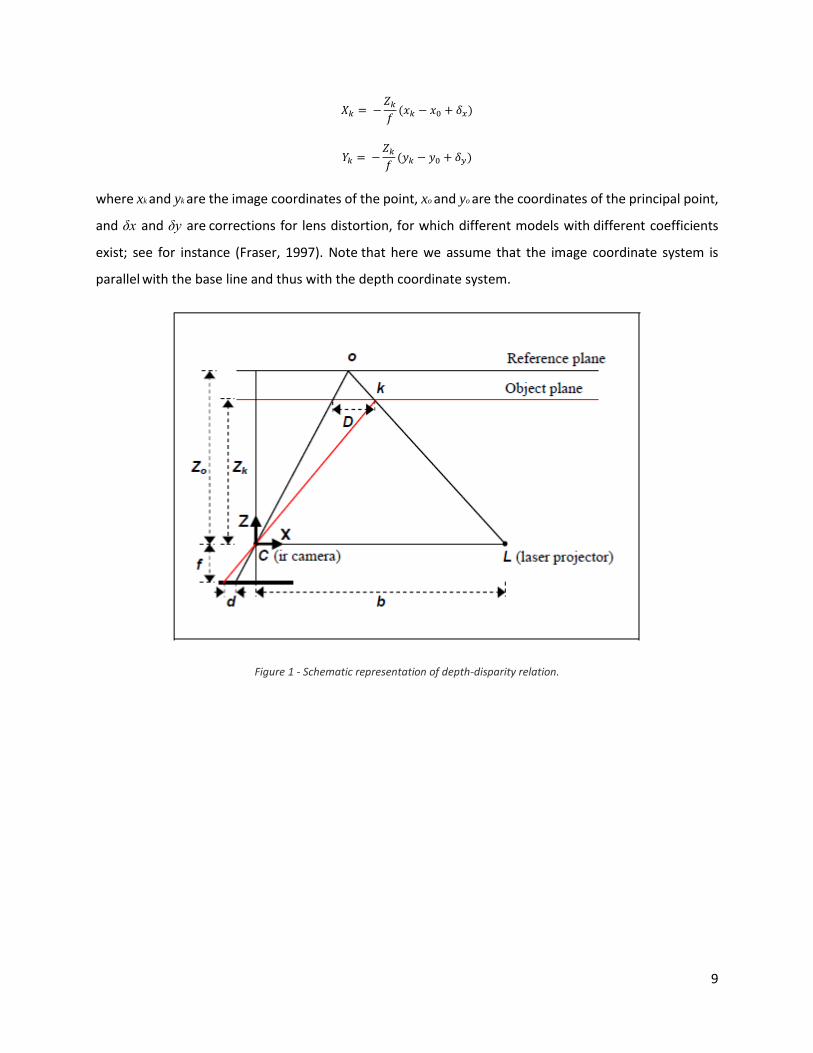
𝑋𝑘 = −𝑍𝑘

𝑓(𝑥𝑘 − 𝑥0 + 𝛿𝑥)

𝑌𝑘 = −𝑍𝑘

𝑓(𝑦𝑘 − 𝑦0 + 𝛿𝑦)

where xk and yk are the image coordinates of the point, xo and yo are the coordinates of the principal point,

and δx and δy are corrections for lens distortion, for which different models with different coefficients

exist; see for instance (Fraser, 1997). Note that here we assume that the image coordinate system is

parallel with the base line and thus with the depth coordinate system.

Figure 1 - Schematic representation of depth-disparity relation.

10

1.2 KINECT XBOX ONE

The Kinect 2 is a time of flight camera that uses the round trip time of light for the calculation of the depth

of an object. Before this camera, offers were all very expensive so 3DV Systems (and Canesta) found a

way to produce a RGB-Depth sensor, called Zcam, at a much lower price, under $ 100. The Microsoft

bought the company before the sensor was launched in the market, thus exploiting it to design the new

Kinect.

FEATURE KINECT 360 KINECT ONE

COLOR CAMERA 640 x 480 @ 30 fps 1920 x 1080 @ 30 fps

CAMERA DEPTH 320 x 240 512 x 424

MAXIMUM DEPTH DISTANCE ~4.5m ~4.5m

MINIMUM DEPTH DISTANCE 40 cm 50 cm

HORIZONTAL FIELD OF VIEW 57 degrees 70 degrees

VERTICAL FIELD OF VIEW 43 degrees 60 degrees

TILT MOTOR Yes no

SKELETON JOINTS DEFINED 20 26

PERSON TRACKED 2 6

USB 2.0 3.0

11

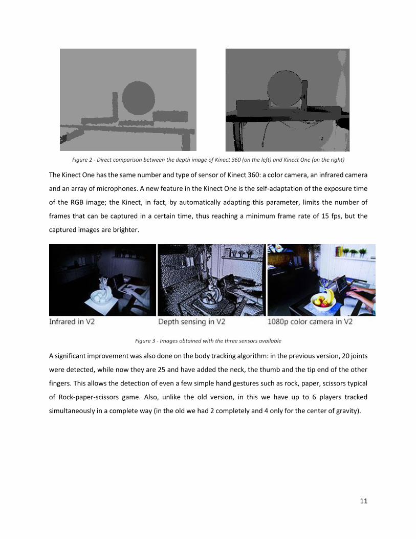
Figure 2 - Direct comparison between the depth image of Kinect 360 (on the left) and Kinect One (on the right)

The Kinect One has the same number and type of sensor of Kinect 360: a color camera, an infrared camera

and an array of microphones. A new feature in the Kinect One is the self-adaptation of the exposure time

of the RGB image; the Kinect, in fact, by automatically adapting this parameter, limits the number of

frames that can be captured in a certain time, thus reaching a minimum frame rate of 15 fps, but the

captured images are brighter.

Figure 3 - Images obtained with the three sensors available

A significant improvement was also done on the body tracking algorithm: in the previous version, 20 joints

were detected, while now they are 25 and have added the neck, the thumb and the tip end of the other

fingers. This allows the detection of even a few simple hand gestures such as rock, paper, scissors typical

of Rock-paper-scissors game. Also, unlike the old version, in this we have up to 6 players tracked

simultaneously in a complete way (in the old we had 2 completely and 4 only for the center of gravity).

12

Figure 4 – Skeleton joints defined and hand gestures detected

The higher resolution of the sensor can capture a mesh of the face of about 2000 points, with 94 units

shape, allowing the creation of avatars closer to reality.

Figure 5 - Points used in the creation of the 3D model

For each detected person, you can know if he is looking at the camera or not (Engaged), his expressions

(happy or neutral), his appearance (if wearing glasses, his skin color or hair) and his activities (eyes open

or closed and mouth open or closed).

13

1.2.1 Principle of depth measurement by time of flight

The [2] well explain how the Kinect One works. Figure 62 shows the 3D image sensor system of Kinect One.

The system consists of the sensor chip, a camera SoC, illumination, and sensor optics. The SoC manages

the sensor and communications with the Xbox One console. The time-of-flight system modulates a camera

light source with a square wave. It uses phase detection to measure the time it takes light to travel from

the light source to the object and back to the sensor, and calculates distance from the results. The timing

generator creates a modulated square wave. The system uses this signal to modulate both the local light

source (transmitter) and the pixel (receiver). The light travels to the object and back in time Δ𝑡. The system

calculates Δ𝑡 by estimating the received light phase at each pixel with knowledge of the modulation

frequency. The system calculates depth from the speed of light in air: 1 cm in 33 picoseconds.

Figure 6 - 3D image sensor system. The system comprises the sensor chip, a camera SoC, illumination, and sensor optics.

2 Picture got from [2]

14

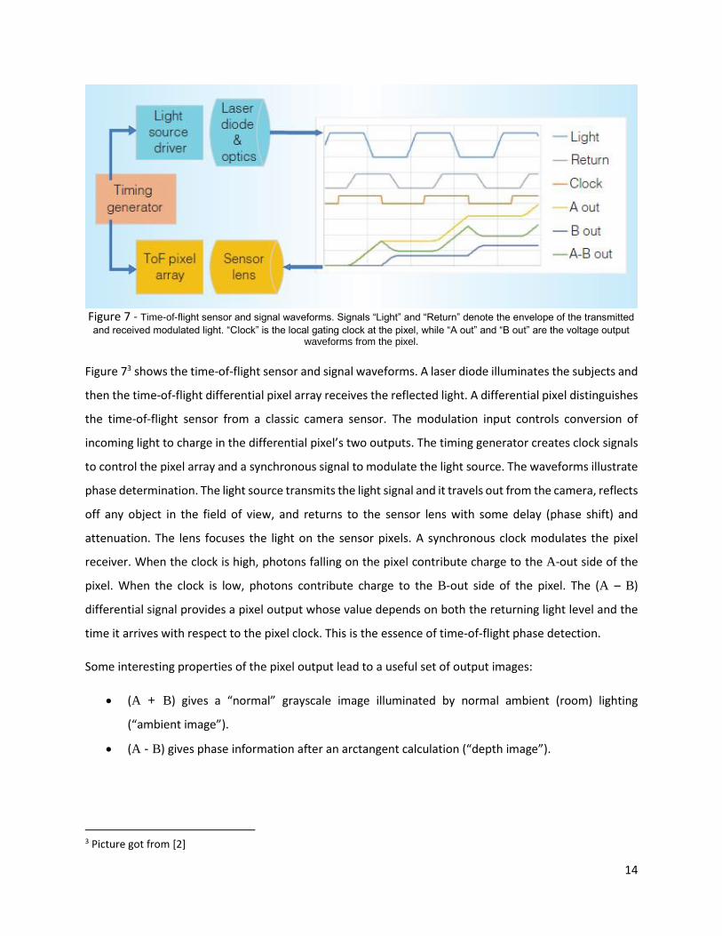
Figure 7 - Time-of-flight sensor and signal waveforms. Signals “Light” and “Return” denote the envelope of the transmitted

and received modulated light. “Clock” is the local gating clock at the pixel, while “A out” and “B out” are the voltage output waveforms from the pixel.

Figure 73 shows the time-of-flight sensor and signal waveforms. A laser diode illuminates the subjects and

then the time-of-flight differential pixel array receives the reflected light. A differential pixel distinguishes

the time-of-flight sensor from a classic camera sensor. The modulation input controls conversion of

incoming light to charge in the differential pixel’s two outputs. The timing generator creates clock signals

to control the pixel array and a synchronous signal to modulate the light source. The waveforms illustrate

phase determination. The light source transmits the light signal and it travels out from the camera, reflects

off any object in the field of view, and returns to the sensor lens with some delay (phase shift) and

attenuation. The lens focuses the light on the sensor pixels. A synchronous clock modulates the pixel

receiver. When the clock is high, photons falling on the pixel contribute charge to the A-out side of the

pixel. When the clock is low, photons contribute charge to the B-out side of the pixel. The (A – B)

differential signal provides a pixel output whose value depends on both the returning light level and the

time it arrives with respect to the pixel clock. This is the essence of time-of-flight phase detection.

Some interesting properties of the pixel output lead to a useful set of output images:

(A + B) gives a “normal” grayscale image illuminated by normal ambient (room) lighting

(“ambient image”).

(A - B) gives phase information after an arctangent calculation (“depth image”).

3 Picture got from [2]

15

√∑(𝐴 − 𝐵)2 gives a grayscale image that is independent of ambient (room) lighting (“active

image”).

Chip optical and electrical parameters determine the quality of the resulting image. It does not depend

significantly on mechanical factors. Multiphase captures cancel linearity errors, and simple temperature

compensation ensures that accuracy is within specifications. Key benefits of the time-of-flight system

include the following:

One depth sample per pixel: X – Y resolution is determined by chip dimensions.

Depth resolution is a function of the signal-to-noise ratio and modulation frequency: that is,

transmit light power, receiver sensitivity, modulation contrast, and lens f-number.

Higher frequency: the phase to distance ratio scales directly with modulation frequency resulting

in finer resolution.

Complexity is in the circuit design. The overall system, particularly the mechanical aspects, is

simplified.

An additional benefit is that the sensor outputs three possible images from the same pixel data: depth

reading per pixel, an “active” image independent of the room and ambient lighting, and a standard

“passive” image based on the room and ambient lighting.

The system measures the phase shift of a modulated signal, then calculates depth from the phase using

2𝑑 =𝑝ℎ𝑎𝑠𝑒

2𝜋

𝑐

𝑓𝑚𝑜𝑑 , where depth is d, c is the speed of light, and fmod is the modulation frequency.

Increasing the modulation frequency. Increasing the modulation frequency increases resolution —that is,

the depth resolution for a given phase uncertainty. Power limits what modulation frequencies can be

practically used, and higher frequency increases phase aliasing.

Phase wraps around at 360°. This causes the depth reading to alias. For example, aliasing starts at a depth

of 1.87 m with an 80-MHz modulation frequency. Kinect acquires images at multiple modulation

frequencies (see Figure 8). This allows ambiguity elimination as far away as the equivalent of the beat

frequency of the different frequencies, which is greater than 10 m for Kinect, with the chosen frequencies

of approximately 120 MHz, 80 MHz, and 16MHz.

16

Figure 84 - Phase to depth calculation from multiple modulation frequencies. Each individual single-frequency phase result

(vertical axis) produces an ambiguous depth result (horizontal axis), but combining multiple frequency results disambiguates the result.

Finally the device is also able to acquire at the same time two images with two different shutter times of

100[µ]s and 1000[µ]s. The best exposure time is selected on the fly for each pixel.

Figure 9 - Basic operation principle of a Time-Of-Flight camera

1.2.2 Driver and SDK

The SDK provides all the tools necessary to acquire data through the Kinect by classes, functions and

structures that manage the dialogue with the sensors.

Classes and functions in the SDK can be grouped into these main categories:

Audio. Classes and functions to communicate with the microphone that allow you to record audio

and to know the direction and the person who generated.

Color camera full HD. Classes and functions to capture images from the camera.

Depth image. Classes and functions to capture the depth image.

4 Picture got from [2]

17

Infrared image. Classes and functions to capture the infrared image of the scene; it is also

possible to request a picture with a greater exposure time which is better, both for the best level

of detail, both for the lower presence of noise.

Face. Classes and functions to detect the person's face, some key points as eyes and mouth and

detect the expressions.

FaceHD. Classes and functions to get the color of skin, hair, and useful points to create a mesh of

the face.

Coordinate calculation. Classes and function for calculate the points’ coordinate between images

acquired with different sensors (i.e. from point’s coordinate into RGB image into point’s

coordinate into depth image).

The Kinect. Classes and functions to activate and close the connection with the Kinect and get

information about the status of the device.

1.2.2.1 Acquire new data

To acquire data from Kinect, the steps to follow can be summarized.

1. Initialize the object that communicates with the device detecting the Kinect connected.

2. Open the connection with the Kinect.

3. Get the reader for the data source (BodyFrameSource->OpenReader())

4. Set the function that will handle the event when new data from the device.

5. Handle the new data.

6. Close the connection with the Kinect.

Figure 10 - Phases for the acquisition of data

The Source give the frame from which you can get the data. Data access can be done by two methods: by

going directly to the buffer, thus avoiding a copy of the data, or by copying the data into an array.

Sensor Source Frame Data

18

1.2.2.2 Body tracking

The tracking of people is very important and deserves attention. The SDK Kinect returns an array

containing objects representing the people detected, each object contains information on the joints of

the body, on the state of the hands and other information.

The code below shows an example of how we proceed to open a connection to the sensor, it records the

event and fills the array with the information about the bodies found. The structure follows the approach

followed for the other sensors.

The information on the skeleton are oriented as if the person was looking in a mirror to facilitate

interaction with the world.

As an example, if the user touches an object with the right hand, the information on this gesture is

provided by the corresponding joints:

JointType::HandRight

JointType::HandTipRight

JointType::ThumbRight

For each joint of the skeleton there is a normal which describes its rotation. The rotation is expressed as

a vector (oriented in the world) perpendicular with the bone in the hierarchy of the skeleton. For example,

to determine the rotation of the right elbow, using the parent in the hierarchy of the skeleton, the right

shoulder, to determine the plane of the bone and determine the normal with respect to it.

void MainPage::InitKinect() { KinectSensor^ sensor = KinectSensor::GetDefault(); sensor->Open(); bodyReader = sensor->BodyFrameSource->OpenReader(); bodyReader->FrameArrived += ref new EventHandler<typename BodyFrameArrivedEventArgs^> (this, &MainPage::OnBodyFrameArrived); bodies = ref new Platform::Collections::Vector<Body^>(6); } void MainPage::OnBodyFrameArrived(BodyFrameReader ^sender, BodyFrameArrivedEventArgs ^eventArgs){ BodyFrame ^frame = eventArgs->FrameReference->AcquireFrame(); if (frame != nullptr){ frame->OverwriteBodyData(bodies); } }

19

The hierarchy of the skeleton starts from the center of the body and extends at its ends, from the upper

to the lower joint; This connection is described from bones. For example, the bones of the right arm (not

including the thumb) consist of the following connections:

Right hand - Tip of the right hand

Right elbow - Right Wrist

Right Shoulder - Elbow Right

Hands contain additional information and for every hand you can know the status of the available (open

hand, closed hand gesture of the scissors, untracked, unknown).This allows us to understand how the user

is interacting with the world that surrounds him and to provide a system which responds to only one

movement of the hand.

1.2.2.3 Face tracking

With the available APIs, a lot of information from the user's face can be extracted. There are two groups

of objects, which provide access to different information, and we can identify with: High definition face

tracking and face tracking. Classes and functions in the first group acquire information on the face, as the

area occupied by the face in the color and infrared, the main points of the face (position of the eyes, the

nose and the corners of the mouth ) and the rotation of the face. In the image below, you can see the

expressions that are detected and their reproduction on a 3D model of the face made via Kinect.

20

Figure 11 - Expressions detected by the Kinect and their reproduction on a model's face

The second group includes all the functions and classes to create a 3D model of the face and animate it.

The animation API recognizes up to 17 units (AUs), which are expressed as a number value which varies

between 0 and 1, and 94 shape units (SUs), also associated to a weight that varies between -2 and 2. The

weight the various points indicates how to modify the model's face for animation.

The model of the face can be calculated directly using the functions of the SDK and then you can access

the triangle vertices of the mesh. The points used to calculate the model are those visible in Figure 5

21

Figure 12 - Example of face made via Kinect

Figure 13 - 3D face after it is applied to the color mesh of the face

22

1.2.3 Survey of Open Source Drivers and SDKs

1.2.3.1 IAI-Kinect

The IAI Kinect package is a set of tools and libraries that make possible to use the Kinect One within ROS

(Robot Operating System5). The project is still under development but it aims to make available all the

features that were usable with the first Kinect and it depends on the evolution of the libfreenect2 driver

which is under development too.

The combination consists of:

Camera calibration: a tool of calibration to calculate the intrinsic parameters whether of the

infrared camera whether of the colour one;

A library for aligning depth and color information with support for OpenCL;

kinect2_bridge: a medium between ROS and libfreenect2;

registration_viewer: a viewer for images and point cloud.

Figure 14 - Sample rgb image and depth and point cloud acquired with the IAI-package for Kinect One

5 http://www.ros.org/

23

1.2.3.2 Kinect2 bridge

Kinect2 Bridge is mainly involved in acquiring the data from the Kinect through the libfreenect26 driver

and in publishing them in the topics. The structure of these ones follows ROS standard for the cameras:

camera/sensor/image. So, the following images are published:

RGB/image: the colour image obtained by the Kinect2 with a resolution of 1920x1080 pixels;

RGB_lowres/image: the rectified and undistorted color image, rescaled with a resolution of

960x540 pixels, Full HD’s half;

RGB_rect/image: the rectified and undistorted color image with the same size as the original;

Depth/image: the depth’s image obtained from the Kinect2 with a resolution of 512x424 pixels;

Depth_rect/image: the depth’s image overhauled and warmed up with a resolution of 960x540

pixels;

Depth_lowres/image: the overhauled depth’s image with the same size as the original;

Ir/image: the infrared image reached from the Kinect2 with a resolution of 512x424 pixels;

Ir_lowres/image: the rectified and undistorted color image, rescaled with a resolution of 960x540

pixels;

Ir_rect/image: the rectified and undistorted infrared image with the same size as the original.

To launch Kinect2 Bridge use a command like:

Or

You can also specify some parameters (only available with rosrun) as:

fps which limits the frames per second published;

calib to indicate the folder that contains the calibration parameters, intrinsic and extrinsic;

raw to specify to post pictures of depth as 512x424 instead of 960x540.

The calibration data used are those that can be estimated using the calibration package available in the

repository.

6 https://github.com/OpenKinect/libfreenect2

roslaunch kinect2_bridge kinect2_bridge.launch

rosrun kinect2_bridge kinect2_bridge

24

1.2.3.3 Comparison with the Microsoft SDK

IAI-Kinect uses libfreenect2 as driver to capture data from the Kinect. This driver is open source and

available for all major operating systems. The features offered by this driver are fewer than those of the

Microsoft driver but it is certainly interesting because it allows to extend the use of Kinect One with

operating systems other than Windows. The driver is in development state and allows the acquisition of

color, IR and depth images. IAI-Kinect package does not allow to estimate the body joints and so the

tracking of people; for all applications that need this information, Microsoft’s SDK is the only option.

IAI-Kinect SDK Microsoft

Microphone acquisition No Yes

RGB image acquisition Yes Yes

Depth image acquisition Yes Yes

IR image acquisition Yes Yes

Joint estimation No Yes

Face analysis No Yes

Camera calibration Yes No

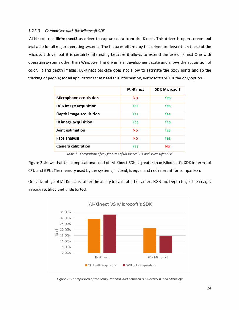
Table 1 - Comparison of key features of IAI-Kinect SDK and Microsoft’s SDK

Figure 2 shows that the computational load of IAI-Kinect SDK is greater than Microsoft’s SDK in terms of

CPU and GPU. The memory used by the systems, instead, is equal and not relevant for comparison.

One advantage of IAI-Kinect is rather the ability to calibrate the camera RGB and Depth to get the images

already rectified and undistorted.

Figure 15 - Comparison of the computational load between IAI-Kinect SDK and Microsoft

0,00%

5,00%

10,00%

15,00%

20,00%

25,00%

30,00%

35,00%

IAI-Kinect SDK Microsoft

load

IAI-Kinect VS Microsoft's SDK

CPU with acquisition GPU with acquisition

25

CPU Intel Core i7 – 4710HQ

RAM 8 GB

GPU NVIDIA GEFORCE GTX 850m

Table 2 - Main features of the PC used for testing

Figure 16 shows instead as the publication and display of the Point Cloud in RVIZ implies to consume

almost all available resources. This high computational cost you pay for real time applications such as

people tracking and following.

Figure 16 - Computational load of IAI-Kinect in Ubuntu

1.2.3.4 Publication of Point Cloud in Kinect2 bridge

The package IAI-Kinect does not have natively publication of Point Clouds generated by the depth and

RGB images so, to make easier the use of algorithms that use the Point Cloud, we inserted the ability to

publish directly this kind of data. This change also allowed a performance increase of about 25% with the

algorithm for tracking people. The following table illustrates the method used to integrate the new feature.

First we declare the publisher:

0,00%

10,00%

20,00%

30,00%

40,00%

50,00%

60,00%

70,00%

80,00%

90,00%

CPU GPU

load

Computational load IAI-Kinect

Acquisition Image in RVIZ Point Cloud in RVIZ

ros::Publisher pub_pointcloud_; pub_pointcloud_=nh.advertise<pcl::PointCloud<pcl::PointXYZRGB>>

("/camera/depth_registered/points", 1);

26

For each frame that is captured by Kinect we calculate a new point cloud:

//**** VARIABLES //matrices with the intrinsic parameters of the camera rgb cv::Mat cameraMatrixColor, cameraMatrixColorLow, distortionColor; //matrices with the intrinsic parameters of the camera depth cv::Mat cameraMatrixDepth, distortionDepth; //matrices with extrinsic parameters cv::Mat rotation, translation; //loockup table for the creation of the point cloud cv::Mat lookupX, lookupY; //matrices for antidistortion and rectification of the acquired images cv::Mat map1Color, map2Color; cv::Mat map1ColorReg, map2ColorReg; cv::Mat map1Depth, map2Depth; //input image cv::Mat rgb, depth; //output image cv::Mat rgb_low, depth_low;

//**** Point cloud creation //create the matrices for antidistortion and rectification of the acquired images cv::initUndistortRectifyMap(cameraMatrixColor, distortionColor, cv::Mat(), cameraMatrixColor,cv::Size(rgb.cols, rgb.rows), mapType, map1Color, map2Color) cv::initUndistortRectifyMap(cameraMatrixColor, distortionColor, cv::Mat(), cameraMatrixDepth, cv::Size(depth.cols, depth.rows), mapType, map1ColorReg, map2ColorReg); cv::initUndistortRectifyMap(cameraMatrixDepth, distortionDepth, cv::Mat(), cameraMatrixDepth, cv::Size(depth.cols, depth.rows), CV_32FC1, map1Depth, map2Depth); //antidistort and rectificate the images cv::remap(rgb, rgb, map1Color, map2Color, cv::INTER_NEAREST); cv::remap(depth, depth, map1Depth, map2Depth, cv::INTER_NEAREST); cv::remap(rgb, rgb_low, map1ColorReg, map2ColorReg, cv::INTER_AREA); // flip images horizontally cv::flip(rgb_low,rgb_low,1); cv::flip(depth_low,depth_low,1); //create the loock up table createLookup(rgb_low.cols, rgb_low.rows); //create the point cloud createCloud(depth_low, rgb_low, output_cloud);

27

void createLookup(size_t width, size_t height) { const float fx = 1.0f / cameraMatrixDepth.at<double>(0, 0); const float fy = 1.0f / cameraMatrixDepth.at<double>(1, 1); const float cx = cameraMatrixDepth.at<double>(0, 2); const float cy = cameraMatrixDepth.at<double>(1, 2); float *it; lookupY = cv::Mat(1, height, CV_32F); it = lookupY.ptr<float>(); for(size_t r = 0; r < height; ++r, ++it) { *it = (r - cy) * fy; } lookupX = cv::Mat(1, width, CV_32F); it = lookupX.ptr<float>(); for(size_t c = 0; c < width; ++c, ++it) { *it = (c - cx) * fx; } }

void createCloud(const cv::Mat &depth, const cv::Mat &color, pcl::PointCloud<pcl::PointXYZRGB>::Ptr &cloud) { const float badPoint = std::numeric_limits<float>::quiet_NaN(); #pragma omp parallel for for(int r = 0; r < depth.rows; ++r) { pcl::PointXYZRGB *itP = &cloud->points[r * depth.cols]; const uint16_t *itD = depth.ptr<uint16_t>(r); const cv::Vec3b *itC = color.ptr<cv::Vec3b>(r); const float y = lookupY.at<float>(0, r); const float *itX = lookupX.ptr<float>(); for(size_t c = 0; c < (size_t)depth.cols; ++c, ++itP, ++itD, ++itC, ++itX) { register const float depthValue = *itD / 1000.0f; // Check for invalid measurements if(isnan(depthValue) || depthValue <= 0.001) { // not valid itP->x = itP->y = itP->z = badPoint; } else { itP->z = depthValue; itP->x = *itX * depthValue; itP->y = y * depthValue; } itP->b = itC->val[0]; itP->g = itC->val[1]; itP->r = itC->val[2]; } } }

28

We add the header to the point cloud for publication and public.

To enable the new feature, we modified the file launcher adding a new parameter: publish_cloud that

must assume a value of true because the point cloud is published.

//create point cloud header cv_bridge::CvImagePtr cv_ptr(new cv_bridge::CvImage); cv_ptr->header.seq = header.seq; cv_ptr->header.stamp = header.stamp; cv_ptr->encoding = "bgr8"; cloud->header.frame_id = "/camera_rgb_optical_frame"; cloud->header = pcl_conversions::toPCL(cv_ptr->header); cloud->header.frame_id = "/camera_rgb_optical_frame"; //pubblish the point cloud pub_pointcloud_.publish(cloud);

<launch> <arg name="publish_frame" default="true" /> <arg name="publish_cloud" default="true" /> <include file="$(find kinect2_bridge)/launch/include/kinect2_frames.launch"> <arg name="publish_frame" value="$(arg publish_frame)" /> </include> <node name="kinect2_bridge" pkg="kinect2_bridge" type="kinect2_bridge" respawn="true"

output="screen"> <param name="publish_cloud" value="$(arg publish_cloud)" /> </node> </launch>

29

2 KINECT RECORDER

Figure 17 - Kinect Recorder main window

The IAI-Kinect package doesn’t allow to acquire all the Kinect data, such as: microphone or body’s joints.

We develop a software that record all the Kinect data and save them to disk for future uses. This software

is called: Kinect Recorder.

2.1 C++ VS C# The SDK allows you to write code with two different languages: C ++ and C #. To see which of the two

allows you to get a better result, we decided to implement the program in both languages and compare

their performance. As seen from Figure 18, the number of frames that can be saved with the solution C

++ is much greater although this too is subject to a variable frame rate but this is due to the operating

system and not to the program.

Figure 18 - Comparison fps program written in C ++ to C # against

0

10

20

30

40

C++ VS C#

C++ monothread C# monothread

30

2.2 OPTIMAL SOLUTION The program written in C ++ monothread managed to get to as many as 21 fps, sufficient for a good

number of applications but, as can be seen from Figure 18, not stable over time. To correct this behavior

we have adopted a series of measures. We first entered a buffer for temporary storage of data acquired

from the Kinect, delegating emptying the buffer to other threads writers. The structure of the application

then becomes the following:

This idea turned out to be good, in fact we could save all the frames, reaching 30 fps stable, but rapidly

saturating the available memory. The data heavier to store is the RGB image that is 8MB (1920x1080 pixels

with 4 channel). For correct this side effect we use another buffer and threads that, before insert the data

for writing, encode the color image to JPEG. A single JPEG image weight about 400 KB, thus the memory

saving is big.

The final structure of the program is then the following:

The final program is able to save all the data, stably.

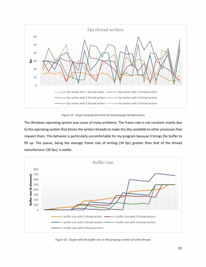
For optimum performance these measures are not sufficient, but you also need a proper balance between

the number of threads that deal with various roles. As seen from the graph in Figure 19, to a greater

number of threads do not always match the improvements, in fact, using 6 thread writers, you get lower

performance that 5. This is probably due to the overhead of the high number of threads. The best

performance is reached using: 1 thread manufacturer, 2 threads for encoding and 5 for writing.

Producer

•It acquires data from kinect

Buffer for writing

•It maintains data to write to disk

Thread writers

•Empty the buffer by writing data to disk

Producer

•It acquires data from kinect

Buffer for compression

•It secures the data to be compressed

Thread encoder

•Encode RGB images in JPEG

Buffer for writing

•It maintains data to write to disk

Thread writers

•Empty the buffer by writing data to disk

31

Figure 19 - Graph showing the trend of increasing fps thread writers

The Windows operating system was cause of many problems. The frame rate is not constant mainly due

to the operating system that blocks the writers threads to make the disc available to other processes that

request them. This behavior is particularly uncomfortable for my program because it brings the buffer to

fill up. The queue, being the average frame rate of writing (34 fps) greater than that of the thread

manufacturer (30 fps), is stable.

Figure 20 - Graph with the buffer size on the growing number of write threads

0

10

20

30

40

50

60

fps

Fps thread writers

c++ fps writer with 1 thread writer c++ fps writer with 2 thread writers

c++ fps writer with 3 thread writers c++ fps writer with 5 thread writers

c++ fps writer with 5 thread writers c++ fps writer with 6 thread writers

0

100

200

300

400

500

600

700

800

Bu

ffe

r si

ze (

# e

lem

en

t)

Buffer size

c++ buffer size with 1 thread writer c++ buffer size with 2 thread writers

c++ buffer size with 3 thread writers c++ buffer size with 4 thread writers

c++ buffer size with 5 thread writers

32

2.3 THE CODE Now we analyze the code written for recording data; we use the C ++ code to describe the work done but

the alternative in C # has the same structure. We used the thread offered by C ++ 11 and OpenCV to

process and save the images in order to obtain a code as more portable and reusable.

2.3.1 Initialization

First initialize the object that identifies the Kinect.

I open the connection to the device.

There are several FrameReader that allow access to individual sensors (eg. AudioFrameReader) and obtain

the captured frames; in our case, having to access multiple sensors, we use a MultiSourceFrameReader.

2.3.2 Update

The update cycle is the heart of the program and is responsible for acquiring the MultiSourceFrame and

break it down into frame sensors.

We initialize the necessary objects.

We acquire frames.

We break in the frame of the sensors (hereinafter monster an example for the frame depth).

GetDefaultKinectSensor(&m_pKinectSensor);

m_pKinectSensor->Open();

m_pKinectSensor->OpenMultiSourceFrameReader( FrameSourceTypes::FrameSourceTypes_Depth | FrameSourceTypes::FrameSourceTypes_Color | FrameSourceTypes::FrameSourceTypes_BodyIndex | FrameSourceTypes::FrameSourceTypes_Body, &m_pMultiSourceFrameReader);

IMultiSourceFrame* pMultiSourceFrame = NULL; IDepthFrame* pDepthFrame = NULL; IColorFrame* pColorFrame = NULL; IBodyIndexFrame* pBodyIndexFrame = NULL; IBodyFrame* pBodyFrame = NULL;

m_pMultiSourceFrameReader->AcquireLatestFrame(&pMultiSourceFrame);

33

We apply the same procedure for all sensors.

We extracted information from the sensors, which are useful for further processing and checks that

everything went the right way, as the size of the scanned image and the time in which the acquisition took

place.

Finally we access to the image; access is made directly to the buffer used to store the data acquired and

no additional copy.

The example refers to the depth sensor, but a similar process applies also to obtain other data.

2.3.3 Processing

The data obtained are processed and arranged for the rescue disk. All this is done by the method

ProcessFrame which receives at input all the information to save. The method checks if recording is active

or not, if it is active, prepares the data and puts them in a queue for the compression and the next save,

otherwise, refresh the screen visible to the user.

2.3.4 Encoding RGB image

We used the encoding tools provided by OpenCV, and in particular the function imencode that transforms

an image (represented by a cv::Mat) into an unsigned character array, for converting RGB image with JPEG.

The code below exemplifies the data extraction process from the buffer for encoding and then inserting

in the writing buffer.

IDepthFrameReference* pDepthFrameReference = NULL; hr = pMultiSourceFrame->get_DepthFrameReference(&pDepthFrameReference); if (SUCCEEDED(hr)) { hr = pDepthFrameReference->AcquireFrame(&pDepthFrame); } SafeRelease(pDepthFrameReference);

pDepthFrame->AccessUnderlyingBuffer(&nDepthBufferSize, &pDepthBuffer);

34

2.3.5 Saving

When there is some data in the queue, the threads extract the data and write them to disk.

2.3.5.1 Saving RGB image

We write the color image directly through the writing of a binary file. The function provides an input vector

of unsigned char representing the compressed image, its size, and the name of the file to store the data.

2.3.5.2 Saving depth image

To better manage the depth images and facilitate their loading we wrote a special class (DepthImage) that

converts the data into an OpenCV Mat and provides useful methods to save and reload the file. Moreover,

as already mentioned, it is useful to save a map that allows to establish the correspondence between the

points of the color image and the depth; this correspondence is directly provided by the Kinect’s SDK. For

convenience, we wrote a class that handles this aspect and allows saving the map, its loading and the

calculation of the function for a point of interest. These classes are also useful in the reconstruction phase

of the saved data. The depth image is saved as a PGM, that is the format best suited for that type of

information; each image pixel occupies two bytes and contains the distance from the detected object. The

PGM format is a compressed format that preserves the information unchanged. By opening the image

kinect_data* data = vDataToConvert.front(); vDataToConvert.pop_front(); //remove element from from queue lck.unlock();//release the lock cv::Mat t(1080,1920,CV_8UC4,data->pColorBuffer); std::vector<uchar>* output = new std::vector<uchar>; cv::imencode(".jpeg", t, *output); data->pColorBufferConverted = output; delete[] data->pColorBuffer; data->pColorBuffer = NULL; lck.lock(); vData.push_back(data); condition_variable.notify_all(); lck.unlock();

HRESULT SaveJpegToFile(std::vector<uchar>* pBitmapBits, LONG lWidth, LONG lHeight, std::string sFilePath) { int iLen=lWidth*lHeight; std::ofstream out; out.open(sFilePath,std::ofstream::binary); out.write(reinterpret_cast<const char*>(pBitmapBits->data()), pBitmapBits->size()); out.close(); return S_OK; }

35

with softwares like GIMP, the content of the file can also be directly displayed as an image. The map,

instead, is saved in binary format for efficiency reasons.

2.3.5.3 Saving skeleton joints

To save the skeleton joints, we directly extracte the data of interest and concatenate them into a set of

strings ready to be written. During the update, we extracte the information of the skeletons found and

we store them into an array.

We wrote the function (bodyToStr) to compose the final string to save. The function has in input the

bodies’s array and returns the string to save.

HRESULT SaveDepth(UINT16* pDepthBuffer, ColorSpacePoint* pDepthToColorMap, std::string sPathDepthImg, std::string sPathMap) { DepthImage depth(pDepthBuffer); depth.saveToFile(sPathDepthImg); DepthToColorMap::saveMappingToFile(pDepthToColorMap, sPathMap); return S_OK; }

IBody* ppBodies[BODY_COUNT] = {0}; pBodyFrame->GetAndRefreshBodyData(_countof(ppBodies), ppBodies);

36

HRESULT KinectRecorder::bodyToStr(int nBodyCount, IBody** ppBodies, std::string* sOut) { HRESULT hr = S_OK; Joint joints[JointType_Count]; JointOrientation jointsOrientation[JointType_Count]; D2D1_POINT_2F jointPoints[JointType_Count]; for (int i = 0; i < nBodyCount; ++i) { sOut[i] = ""; IBody* pBody = ppBodies[i]; if (pBody) { BOOLEAN bTracked = false; hr = pBody->get_IsTracked(&bTracked); if (SUCCEEDED(hr) && bTracked) { hr = pBody->GetJoints(_countof(joints), joints); if (SUCCEEDED(hr)) { hr = pBody->GetJointOrientations(

_countof(jointsOrientation),jointsOrientation); } if (SUCCEEDED(hr)) { for (int j = 0; j < _countof(joints); ++j) { DepthSpacePoint depthPointPosition = {0}; _pCoordinateMapper->MapCameraPointToDepthSpace( joints[j].Position, &depthPointPosition); DWORD clippedEdges; pBody->get_ClippedEdges(&clippedEdges); int ucOrientation_start=ORIENTATION_JOINT_START[j]; int ucOrientation_end = j; sOut[i] += std::to_string(i+1) + "," + std::to_string(joints[j].Position.X) + "," + std::to_string(joints[j].Position.Y) + "," + std::to_string(joints[j].Position.Z) + "," + std::to_string(depthPointPosition.X) + "," + std::to_string(depthPointPosition.Y) + "," + std::to_string((int)joints[j].TrackingState) + "," + std::to_string((int)clippedEdges) + "," + std::to_string(ucOrientation_start) + "," + std::to_string(ucOrientation_end) + "," + std::to_string(jointsOrientation[j].Orientation.x)+","+ std::to_string(jointsOrientation[j].Orientation.y)+",”+

std::to_string(jointsOrientation[j].Orientation.z)+","+ std::to_string(jointsOrientation[j].Orientation.w)+"\n"; } } } } } return S_OK; }

37

For creating this string, we run through the joints and, for each joint, we concatenate the following

information:

Id of the detected user that owns the joint

World joint position (X, Y, Z);

Depth joint position (X, Y);

TrackingState indicating whether the joint is visible, inferred or unknown;

ClippedEdges that indicates whether the body is visible or if a part of it comes out of the visual

field, possibly indicating which part of the body is outside of the image;

The upper joint of the bone to which the orientation is referred;

The bottom joint of the bone to which the orientation is referred (it is the same joint);

The orientation of the coupled pair of joints in relation to the bone of the world coordinate system

(X, Y, Z, W)

For each skeleton, we then have 26 strings to write to files. The format string has been chosen to comply

with the standard used for acquiring the BIWI RGBD-ID dataset 7 [3], a dataset for people re-identification

from Kinect data. The concatenated strings are then written to file by the thread that empties the buffer.

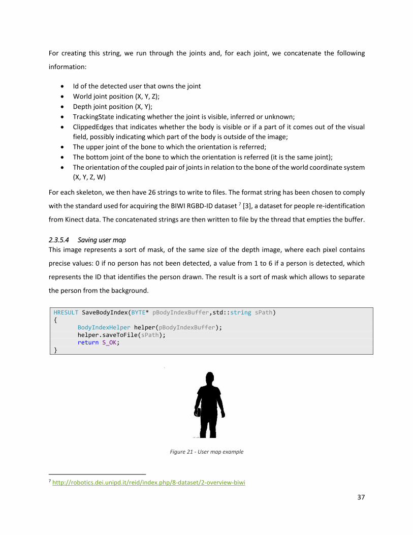
2.3.5.4 Saving user map

This image represents a sort of mask, of the same size of the depth image, where each pixel contains

precise values: 0 if no person has not been detected, a value from 1 to 6 if a person is detected, which

represents the ID that identifies the person drawn. The result is a sort of mask which allows to separate

the person from the background.

Figure 21 - User map example

7 http://robotics.dei.unipd.it/reid/index.php/8-dataset/2-overview-biwi

HRESULT SaveBodyIndex(BYTE* pBodyIndexBuffer,std::string sPath) { BodyIndexHelper helper(pBodyIndexBuffer); helper.saveToFile(sPath); return S_OK; }

38

2.3.5.5 Saving infrared image

Also the infrared image is saved to a PGM file and, for convenience, we use the same class of the depth

image (DepthImage).

2.3.5.6 Saving floor coefficients

Another important piece of information that is directly provided by the Kinect and that is useful to save is

represented by the coefficients of the plane representing the floor. These coefficients are stored in a plain

text file.

HRESULT SaveInfrared(UINT16* pInfraredBuffer, std::string sPathInfrared) { DepthImage depth(pInfraredBuffer); depth.saveToFile(sPathInfrared); return S_OK; }

HRESULT SaveGroundCoef(const Vector4* coef, std::string sPath) { std::string input; std::cin >> input; std::ofstream out(sPath); out << coef->x << "," << coef->y << "," << coef->z << "," << coef->w; out.close(); return S_OK; }

39

3 SENSORS COMPARISON

In this section, we show a series of tests that compare the Kinect 360 and Kinect One. These tests allow

to highlight the advantages of the second generation of the Kinect. Test in controlled artificial light

A key aspect for RGB-D cameras is the resistance to illumination changes: the acquired data should be

independent of the lighting of the scene. To analyse the behaviour of the depth sensor, a series of images

were acquired in different lighting conditions: no light, low light, neon light and bright light (a lamp

illuminating the scene with 2500W). The set of depth images were then analysed to obtain data useful for

the comparison; in particular, we have created three new images: an image of the standard deviation of

the points, one with the variance and one with the entropy. The variance is defined as 𝜎2 = ∑(𝑥𝑖−�̅�)2

𝑁𝑖 ,

where �̅� = ∑𝑥𝑖

𝑁𝑁𝑖=0 is the sample mean. The standard deviation is simply the square root of the variance

and is therefore defined as 𝜎 = √𝜎2 = √∑(𝑥𝑖−�̅�)2

𝑁𝑖 .

The entropy of a signal can be calculated as 𝐻 = − ∑ 𝑃𝑖(𝑥) log 𝑃𝑖(𝑥)𝑖 , where 𝑃𝑖(𝑥) is the probability that

the pixel considered assumes a given value 𝑥. By applying the definition to the individual pixels the images

that follows are obtained.

3.1.1.1 Kinect 1

Figure 22 - Standard deviation and variance of the depth image of Kinect 360 in absence of light

40

Figure 23 - Standard deviation of the depth image of Kinect 360 in presence of intense light

Figure 24 - Entropy of the depth image of Kinect 360. Left: entropy image in absence of light, right: entropy image with bright light.

The Figure 22 illustrate the pixels standard deviation and variance with no light, instead the Figure 22

show the results with a strong light. The entropy image is showed in Figure 24; on the left the result with

no light and on the right the one with strong light. From this images it seems that the depth estimation

process is not influenced by the change of artificial lighting.

By comparing the standard deviation and variance images, we can notice that, especially near the objects

edges, the variance and the deviation increase. This highlights a major difficulty in estimating the depth

of these points. The entropy image is of particular interest; in fact, the entropy can be interpreted as the

value of uncertainty information. From the pictures, it can be seen that the image captured with no light

has lower entropy and therefore less uncertainty; this conclusion is in line with the analysis obtained by

variance and standard deviation. The dark blue and central band, in fact, has shrunk while the lighter one

has increased. This indicates that the estimated depth value varies over time; the light, thus, influences

41

the scanned image. We can also notice the presence of vertical lines of a lighter colour in the image of the

standard deviation, also visible in the entropy image, probably due to the technique used to estimate the

depth.

3.1.1.2 Kinect 2

Figure 25 - Standard deviation and variance of the depth image of Kinect One in absence of light

Figure 26 - Standard deviation of the depth image of Kinect One in presence of intense light

42

Figure 27 - Entropy of the depth image of Kinect One. Left: entropy image obtained in absence of light, right: entropy image obtained with bright light

TheFigure 25 illustrate the pixels standard deviation and variance with no light, instead the Figure 26 show

the results with a strong light. The entropy image is showed in Figure 27; on the left the result with no

light and on the right the one with strong light. Looking at all the images, only the entropy image gives

some useful information: the image captured in absence of light has slightly lower entropy, demonstrating

that the Kinect One works best in the dark but the difference is so minimal that it can be stated that the

new Kinect is immune to artificial light for the acquisition of the depth image. In this picture, a radial

gradation of color can be noticed, that denotes that depth is less accurate at the edges of the image. The

difference compared to the Kinect 360 is probably due to the different method of calculation.

By comparing the image entropy of the new Kinect with that obtained from the first one, it can be seen

that the Kinect One generates images with greater entropy: the depth assumes a value which varies more

in time but this may also be due to the higher sensitivity of the sensor.

43

3.1.2 Point cloud comparison

After analyzing the depth images, we compared the point clouds. A ground truth is fundamental to be

used as a reference model; for this purpose, we used a point cloud acquired with a laser scanner.

Figure 28 - Point Cloud acquired with the laser scanner

Figure 29 - Scene used for comparison

For comparison, we used a free program, Cloud Compare 8, which allows you to overlap and compare the

cloud points by the points distance. The distance calculated (as described in [4]) for each point of the point

cloud compared is the Euclidean distance between a point on the model and the nearest neighbour of the

cloud compared.

For comparing each point cloud, this process has been followed:

• Reference and test point clouds are aligned to each other;

• The distance between the point clouds is calculated;

• The points are filtered by imposing a maximum distance of 10 cm;

• A comparison with the reference model is re executed.

8 http://www.danielgm.net/cc/

44

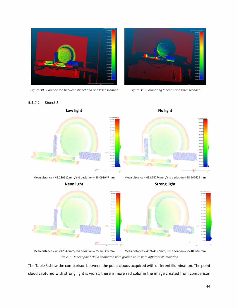
Figure 30 - Comparison between Kinect and one laser scanner

Figure 31 - Comparing Kinect 2 and laser scanner

3.1.2.1 Kinect 1

Low light No light

Mean distance = 45.289112 mm/ std deviation = 25.091047 mm Mean distance = 45.875774 mm/ std deviation = 25.447624 mm

Neon light Strong light

Mean distance = 45.212547 mm/ std deviation = 25.145365 mm Mean distance = 46.974957 mm/ std deviation = 25.400669 mm

Table 3 – Kinect point cloud compared with ground truth with different illumination

The Table 3 show the comparison between the point clouds acquired with different illumination. The point

cloud captured with strong light is worst; there is more red color in the image created from comparison

45

and the mean distance is greater than the others. If we look the mean distance and the standard deviation

value we see that the best result is performed with no light. This test shows how the Kinect 360 is affected

by the change in ambient light, even if the effects are limited and it can still get a good point cloud.

3.1.2.2 Kinect 2

Low light No light

Mean distance = 23.615 mm/ std deviation = 25.498 mm Mean distance = 23.915 mm/ std deviation = 25.620 mm

Neon light Power light

Mean distance = 23.228 mm/ std deviation = 25.310 mm Mean distance = 23.593 mm/ std deviation = 25.446 mm

Table 4 - Kinect point cloud compared with ground truth with different illumination

The Table 4 show the comparison between the point clouds acquired with different illumination. From a

comparison of the point clouds, it is difficult if not impossible to notice the difference in different lighting

condition, thus the new Kinect is almost immune to the change of illumination. It’s interesting to see that

the mean distance and the standard deviation change very little but the best result seems with neon light,

indeed the point cloud with neon light presents the lower mean distance and standard deviation.

46

3.1.3 Results

From the analysis of the previous tests, the results are in line with what was expected. The Kinect is able

to obtain a better result by 48% in the middle range, while retaining a standard deviation unchanged or

even higher. The point cloud of the Kinect One is more precise and better defined for estimating the shape

of the ball. In conclusion, this test showed the advantages of Kinect One, demonstrating precision of point

clouds and invariance to illumination changes.

3.2 OUTDOORS TEST

One of the major advantages of the new technology used in the Kinect One is the possibility to use it in

outdoor environments. Kinect 360 needs to see the pattern it projects on the scene in order to estimate

depth, but this pattern can be strongly altered by the sunlight. Since Kinect One does not have to rely on

this, it results to be less sensitive to external infrared radiation but not entirely immune, also because the

infrared light is still used to calculate depth information by means of the time of flight principle. In this

test, we try to highlight the differences between the cameras and the limitations of both in a real use. This

type of analysis is particularly interesting for applications of people tracking outdoors, which was

impossible with the first generation of Kinect.

3.2.1 Setup

To acquire the data necessary for the comparison, we setup a Pioneer 3-AT robot with both sensors (as

showed in Figure 32). We placed a laptop on a vertical structure installed on the robot, together with a

Kinect 360 and v2 in nearby and solid positions. We also added a laser meter on the top of the robot. We

used the laser meter to determine the approximate location of the Kinects with respect to the reference

object. We chose to install everything on the robot because it allowed to easily move the sensors at

different distances from the objects. As a first step, to get a quick overview of the performances, we

captured different scenes with the two Kinects and compared them (Figure 33); subsequently, some point

clouds were acquired at increasing distances from a wall in the shadow, of a wall in the sun and of a car

in the sun.

The Figure 33 quickly show the difference performance of the Kinects in sun, the new Kinect works well

while the Kinect 360 is blind.

47

Figure 32 - Robot configuration for the acquisition of data

Kinect 1 rgb Kinect 1 Cloud Kinect 2 rgb Kinect 2 Cloud

Figure 33 - Quick comparison between rgb and point cloud at 1.0m e 2.5m from the car

3.2.2 Wall in shadow

The Figure 34 shows the robot position; it was right in front of the wall and was moved at increasing

distance from the wall. The Table 5 shows the acquired point cloud at increasing distance.

Although in an external environment, the lack of direct infrared radiation on the surface of the test allows

both cameras to obtain discrete or even excellent results. The superiority of Kinect One is evident. It can

also be noticed that the point cloud obtained from the Kinect 360 improves with an increasing distance

Kinect2

Kinect 1

PC

Metro laser

P3-AT

48

instead of getting worse as it would be expected. Probably, the infrared sensor saturates for low distances

thus working better at far range.

Figure 34 - Position of the robot when acquiring the data of the wall in shadow

Distance Kinect 1 Kinect 2

0.8 m

1.0 m

1.5 m

49

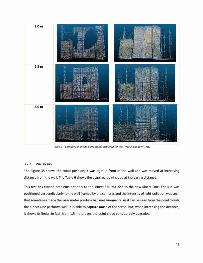
2.0 m

2.5 m

3.0 m

Table 5 – Comparison of the point clouds acquired for the “wall in shadow” test.

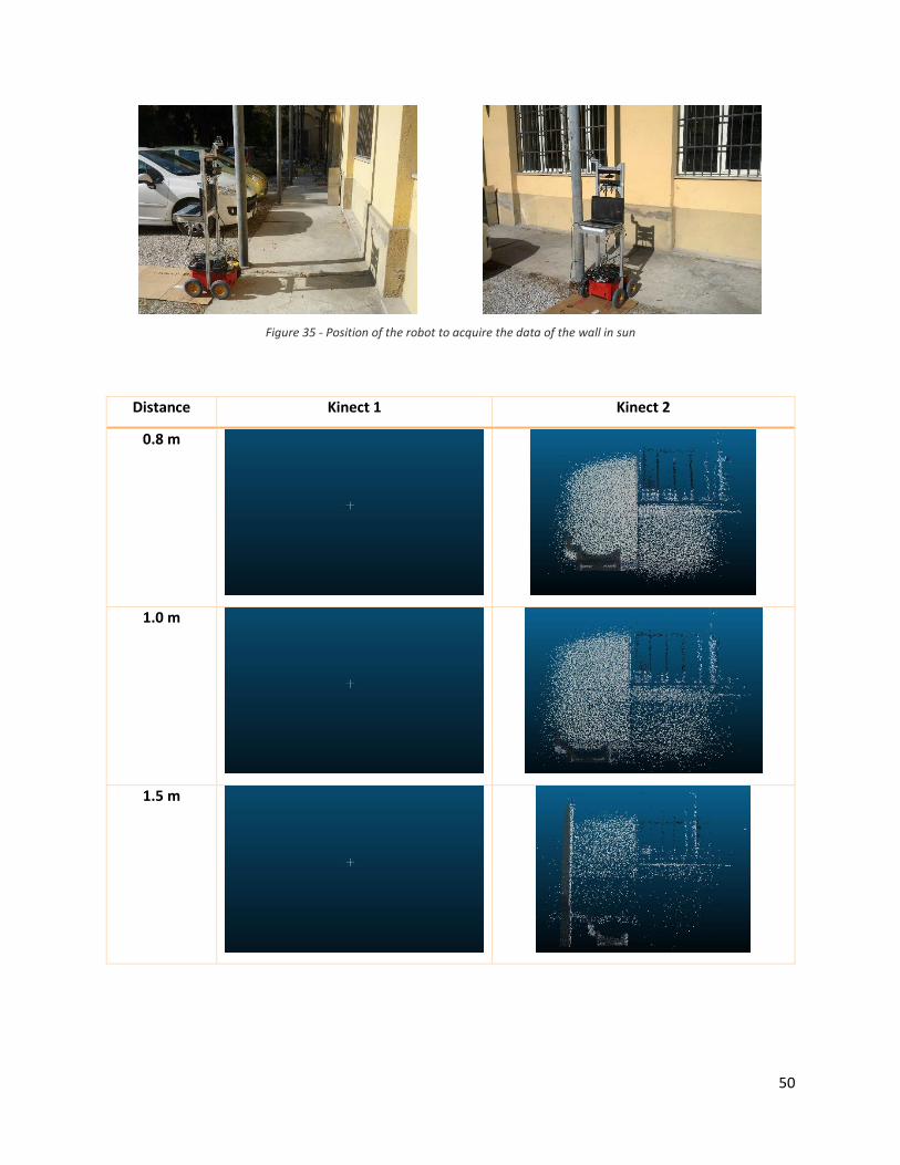
3.2.3 Wall in sun

The Figure 35 shows the robot position; it was right in front of the wall and was moved at increasing

distance from the wall. The Table 6 shows the acquired point cloud at increasing distance.

This test has caused problems not only to the Kinect 360 but also to the new Kinect One. The sun was

positioned perpendicularly to the wall framed by the cameras and the intensity of light radiation was such

that sometimes made the laser meter produce bad measurements. As it can be seen from the point clouds,

the Kinect One performs well: it is able to capture much of the scene, but, when increasing the distance,

it shows its limits. In fact, from 1.5 meters on, the point cloud considerably degrades.

50

Figure 35 - Position of the robot to acquire the data of the wall in sun

Distance Kinect 1 Kinect 2

0.8 m

1.0 m

1.5 m

51

2.0 m

3.0 m

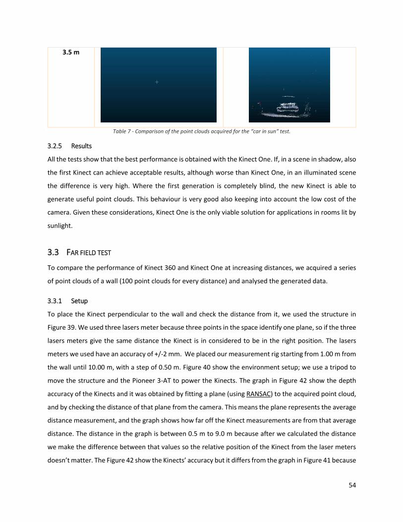
3.5 m

Table 6 - Comparison of the point clouds acquired for the “wall in the sun” test.

3.2.4 Car

After highlighting the limitations of the two cameras, it is interesting to see how they behave in the sun

with a more reflective material. For this purpose, we made the cameras frame a sunlit car. The Figure 36

shows the robot position; it was right in front of the car and was moved at increasing distance. The results

obtained (showed in Table 7) are similar to those already seen but the high reflectivity of the material

allows the Kinect One to obtain a better result compared to the previous test. The sun was not

perpendicular as in the previous test, but was sideward and this influenced the results. In this test,

however, we noticed a typical problem of time of flight cameras: the problem of flying pixels. As it can be

seen from Figure 37, the pixels going from the camera to the subject form flying points that do not exist

in the real scene. This phenomenon is restrained for indoor shots but it is very visible for scenes like this

because of the high presence of natural light. The point cloud can be corrected by an algorithm that

removes non-existing points and interpolates the others to get closer to the original scene. In Figure 37

and Figure 38, we report the point cloud before and after the flying pixels removal.

52

Figure 36 - Position of the robot to acquire the data of the car in sun

Figure 37 - Point Cloud Kinect 2 acquired

Figure 38 - Point Cloud Kinect 2 after removal of flying pixels

53

Distance Kinect 1 Kinect 2

1.0 m

1.5 m

2.0 m

2.5 m

3.0 m

54

3.5 m

Table 7 - Comparison of the point clouds acquired for the “car in sun” test.

3.2.5 Results

All the tests show that the best performance is obtained with the Kinect One. If, in a scene in shadow, also

the first Kinect can achieve acceptable results, although worse than Kinect One, in an illuminated scene

the difference is very high. Where the first generation is completely blind, the new Kinect is able to

generate useful point clouds. This behaviour is very good also keeping into account the low cost of the

camera. Given these considerations, Kinect One is the only viable solution for applications in rooms lit by

sunlight.

3.3 FAR FIELD TEST

To compare the performance of Kinect 360 and Kinect One at increasing distances, we acquired a series

of point clouds of a wall (100 point clouds for every distance) and analysed the generated data.

3.3.1 Setup

To place the Kinect perpendicular to the wall and check the distance from it, we used the structure in

Figure 39. We used three lasers meter because three points in the space identify one plane, so if the three

lasers meters give the same distance the Kinect is in considered to be in the right position. The lasers

meters we used have an accuracy of +/-2 mm. We placed our measurement rig starting from 1.00 m from

the wall until 10.00 m, with a step of 0.50 m. Figure 40 show the environment setup; we use a tripod to

move the structure and the Pioneer 3-AT to power the Kinects. The graph in Figure 42 show the depth

accuracy of the Kinects and it was obtained by fitting a plane (using RANSAC) to the acquired point cloud,

and by checking the distance of that plane from the camera. This means the plane represents the average

distance measurement, and the graph shows how far off the Kinect measurements are from that average

distance. The distance in the graph is between 0.5 m to 9.0 m because after we calculated the distance

we make the difference between that values so the relative position of the Kinect from the laser meters

doesn’t matter. The Figure 42 show the Kinects’ accuracy but it differs from the graph in Figure 41 because

55

it plots the difference between the real value of the plane distance and the calculated one. We calculated

the standard deviation value using the same plane calculated with RANSAC; we got the standard deviation

of the points using the plane’s distance as mean value and we plot the results in the graph in Figure 43.

The precision9 is the repeatability or reproducibility of the measurement, thus we calculated it as the

difference between the minimum and maximum calculated distance value in the acquired frames at the

same distance (this is showed in Figure 44).

The measurement resoluton5 is the smallest change in the underlying physical quantity that produces

a response in the measurement, thus, for every distance, we ordered the data in the point cloud by

growing values and calculate the minimum difference between the acquired depth values. This value is

the resolution of the Kinect and it is shown in Figure 45.

Figure 39 - Platform with three laser meters and a Kinect One

Figure 40 - Test Setup

9 http://en.wikipedia.org/wiki/Accuracy_and_precision

56

3.3.2 Results

Figure 41 – Calculated wall distance

Figure 42 – Kinects’ Accuracy

0,00

1,00

2,00

3,00

4,00

5,00

6,00

7,00

8,00

9,00

10,00

0,00 1,00 2,00 3,00 4,00 5,00 6,00 7,00 8,00 9,00 10,00

Dis

tan

ce m

eas

ure

d (

m)

Right distance (m)

Distance measured

Kinect 360 Kinect One

-0,10

0,00

0,10

0,20

0,30

0,40

0,50

0,60

0,70

0,80

0,00 1,00 2,00 3,00 4,00 5,00 6,00 7,00 8,00 9,00 10,00

Erro

r (m

)

Distance (m)

Accuracy

Kinect 360 Kinect One

57

Figure 43 – Kinects’ standard deviation

Figure 44 – Kinects’ precision

0

0,05

0,1

0,15

0,2

0,25

0 1 2 3 4 5 6 7 8 9 10

Std

dev

(m

)

Distance (m)

Standard deviation

Kinect 360 Kinect One

0

0,05

0,1

0,15

0,2

0,25

0,3

1 1,5 2 2,5 3 3,5 4 4,5 5 5,5 6 6,5 7 7,5 8 8,5 9

Pre

cisi

om

(m

)

Distance (m)

Precision

Kinect 360

Kinect One

58

Figure 45 – Kinects’ resolution

As expected, in Figure 42 and Figure 42, we see that Kinect One achieves better results and the error

remains below the 6 cm in all the measurements, thus Kinect One is better than Kinect 360 in terms of

accuracy. Figure 43 shows that the new Kinect has a lower standard deviation as well. The standard

deviation for Kinect One stays under 1 cm until 7.00 m, indeed the wall in the point cloud is straight and

not corrugated as for the first Kinect. The precision of Kinect 360 (showed in Figure 44) grows with the

distance but not in all steps; this is probably due to quantization errors but a trend can be inferred. The

new Kinect has a better resolution too. Figure 45 shows that the resolution of the Kinect 360 grows a lot

with distance, while the resolution of the new Kinect remains the same in all the measurements. So, for

all the test in far field, the improvements obtained with the new Kinect are very clear.

0

0,05

0,1

0,15

0,2

0,25

0,3

0 2 4 6 8 10

Res

olu

tio

n (

m)

Distance (m)

Resolution

Kinect 360

Kinect One

59

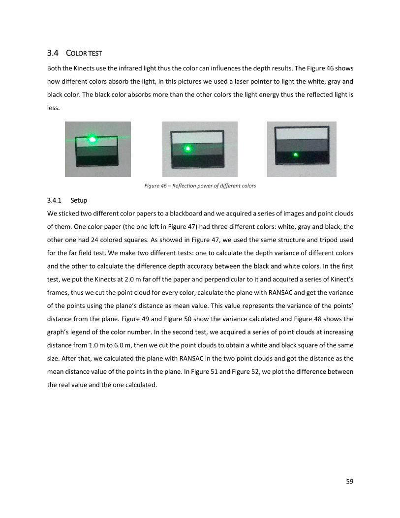
3.4 COLOR TEST

Both the Kinects use the infrared light thus the color can influences the depth results. The Figure 46 shows

how different colors absorb the light, in this pictures we used a laser pointer to light the white, gray and

black color. The black color absorbs more than the other colors the light energy thus the reflected light is

less.

Figure 46 – Reflection power of different colors

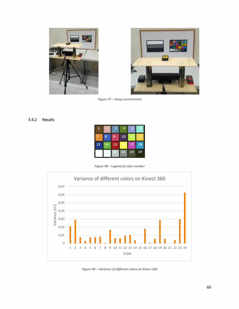
3.4.1 Setup

We sticked two different color papers to a blackboard and we acquired a series of images and point clouds

of them. One color paper (the one left in Figure 47) had three different colors: white, gray and black; the

other one had 24 colored squares. As showed in Figure 47, we used the same structure and tripod used

for the far field test. We make two different tests: one to calculate the depth variance of different colors

and the other to calculate the difference depth accuracy between the black and white colors. In the first

test, we put the Kinects at 2.0 m far off the paper and perpendicular to it and acquired a series of Kinect’s

frames, thus we cut the point cloud for every color, calculate the plane with RANSAC and get the variance

of the points using the plane’s distance as mean value. This value represents the variance of the points’

distance from the plane. Figure 49 and Figure 50 show the variance calculated and Figure 48 shows the

graph’s legend of the color number. In the second test, we acquired a series of point clouds at increasing

distance from 1.0 m to 6.0 m, then we cut the point clouds to obtain a white and black square of the same

size. After that, we calculated the plane with RANSAC in the two point clouds and got the distance as the

mean distance value of the points in the plane. In Figure 51 and Figure 52, we plot the difference between

the real value and the one calculated.

60

Figure 47 – Setup environment

3.4.2 Results

Figure 48 – Legend of color number

Figure 49 – Variance of different colors on Kinect 360

0

0,01

0,02

0,03

0,04

0,05

0,06

0,07

1 2 3 4 5 6 7 8 9 10 11 12 13 14 15 16 17 18 19 20 21 22 23 24

Var

ian

ce (

m2 )

Color

Variance of different colors on Kinect 360

61

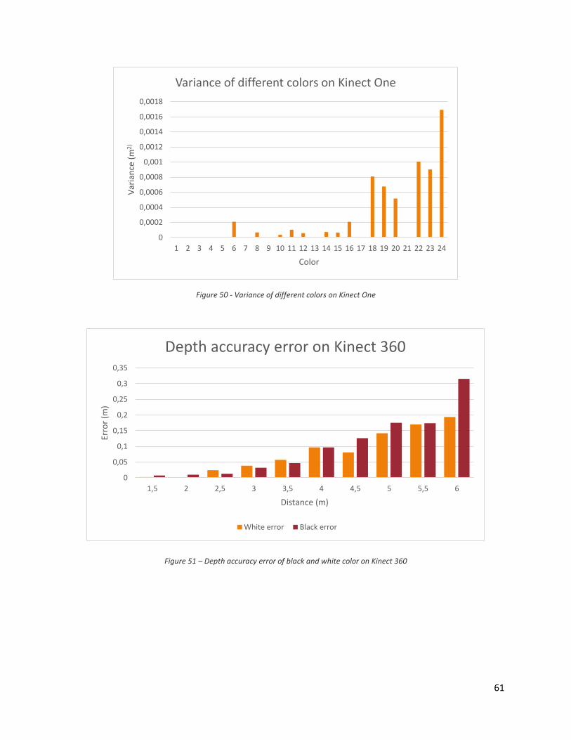
Figure 50 - Variance of different colors on Kinect One

Figure 51 – Depth accuracy error of black and white color on Kinect 360

0

0,0002

0,0004

0,0006

0,0008

0,001

0,0012

0,0014

0,0016

0,0018

1 2 3 4 5 6 7 8 9 10 11 12 13 14 15 16 17 18 19 20 21 22 23 24

Var

ian

ce (

m2

)

Color

Variance of different colors on Kinect One

0

0,05

0,1

0,15

0,2

0,25

0,3

0,35

1,5 2 2,5 3 3,5 4 4,5 5 5,5 6

Erro

r (m

)

Distance (m)

Depth accuracy error on Kinect 360

White error Black error

62

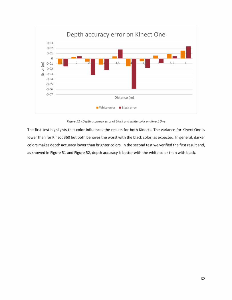
Figure 52 - Depth accuracy error of black and white color on Kinect One

The first test highlights that color influences the results for both Kinects. The variance for Kinect One is

lower than for Kinect 360 but both behaves the worst with the black color, as expected. In general, darker

colors makes depth accuracy lower than brighter colors. In the second test we verified the first result and,

as showed in Figure 51 and Figure 52, depth accuracy is better with the white color than with black.

-0,07

-0,06

-0,05

-0,04

-0,03

-0,02

-0,01

0

0,01

0,02

0,03

1,5 2 2,5 3 3,5 4 4,5 5 5,5 6

Erro

r (m

)

Distance (m)

Depth accuracy error on Kinect One

White error Black error

63

4 APPLICATIONS COMPARISON

4.1 PEOPLE TRACKING AND FOLLOWING

4.1.1 Introduction

People detection and tracking are among the most important perception tasks for an autonomous mobile

robot acting in populated environments. Such a robot must be able to dynamically perceive the world,

distinguish people from other objects in the environment, predict their future positions and plan its

motion in a human aware fashion, according to its tasks.

Techniques of detection and monitoring of people have been extensively studied in the literature, and

many of them use only RGB cameras or 3D sensors but, when working with moving robots, the need for

robustness and real-time capabilities has led researchers to address these problems combining depth and

appearance information.

With the advent of reliable and affordable RGB-D sensors, we have witnessed a rapid boosting of robots

capabilities. Microsoft Kinect 360 sensor allows to natively capture RGB and depth information at good

resolution and frame rate. Even though the depth estimation becomes very poor over eight meters and

this technology cannot be used outdoors, it constitutes a very rich source of information for a mobile

platform.

The Kinect One inherited many of the advantages of the previous version and tries to overcome its

limitations: it manages to detect people up to 10 m away and can be used under the sun. To quantify the

goodness of the new Kinect for these applications, we installed it on a Pioneer 3-AT and we carried out a

number of tests.

64

4.1.2 Pioneer 3-AT

The Pioneer 3-AT is a highly versatile platform on four

wheels, useful for the development of robot navigation

applications.

The P3-AT is equipped with three batteries with 7.2 Ah

capacity each, thus giving a good autonomy to the

robot.

The robot used for the test is equipped with a series of

power plugs of 5 and 12 volt for the connection of

auxiliary devices.

To install the Kinect One on the robot, considering the impossibility to recover the original

plug used by the Kinect, we cut the original power cable and equipped it with a connector

suitable for the connection to the robot. We solved the problem by dividing the power

cord and installing, at the end of the two wires, two plugs (one male and one female) of

5.5 mm that make possible both the use of the original power supply and the connection to the robot.

4.1.3 Setup

The people following application receives as input the people tracking result. For Kinect 360 we used the

people tracking and following software described in [5], which was designed to work within ROS. Then,

we easily adapted this software to also work with Kinect One. In particular, we only had to modify a launch

file o remap the Kinect One topics to the topics used for Kinect 360. To make the robot follow a person

using the Kinect One, we modified some configuration files to reflect the position of the new Kinect. The

main difference we experienced with respect to the Kinect 360, was the lower frame rate of the overall

application, mainly due to the high computational load requested by the Kinect One driver for Ubuntu. In

order to improve the performances and because it was not already present, we integrated the publication

of the point cloud in kinect2_bridge, getting a frame rate increase from 4 fps to 5 fps.

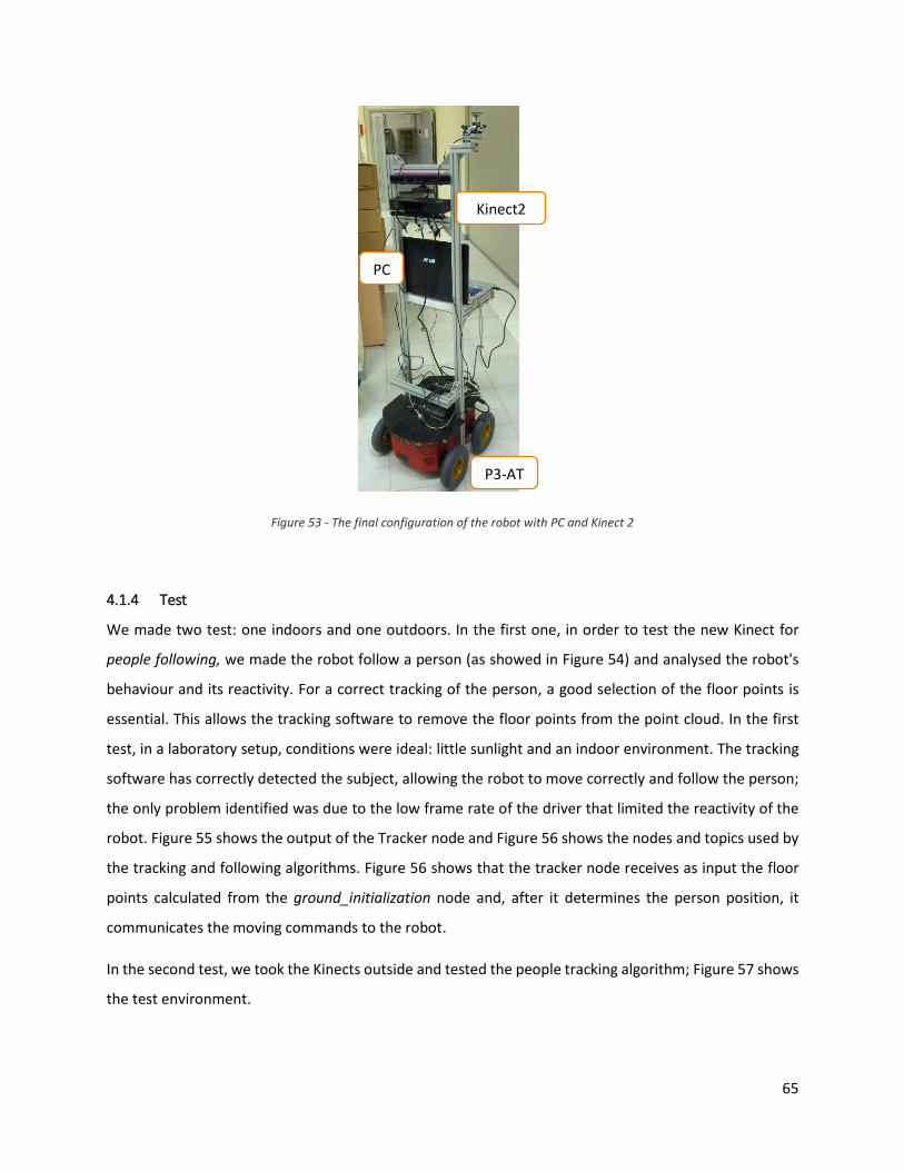
65

Figure 53 - The final configuration of the robot with PC and Kinect 2

4.1.4 Test

We made two test: one indoors and one outdoors. In the first one, in order to test the new Kinect for

people following, we made the robot follow a person (as showed in Figure 54) and analysed the robot's

behaviour and its reactivity. For a correct tracking of the person, a good selection of the floor points is

essential. This allows the tracking software to remove the floor points from the point cloud. In the first

test, in a laboratory setup, conditions were ideal: little sunlight and an indoor environment. The tracking

software has correctly detected the subject, allowing the robot to move correctly and follow the person;

the only problem identified was due to the low frame rate of the driver that limited the reactivity of the

robot. Figure 55 shows the output of the Tracker node and Figure 56 shows the nodes and topics used by

the tracking and following algorithms. Figure 56 shows that the tracker node receives as input the floor

points calculated from the ground_initialization node and, after it determines the person position, it

communicates the moving commands to the robot.

In the second test, we took the Kinects outside and tested the people tracking algorithm; Figure 57 shows

the test environment.

PC

P3-AT

Kinect2

66

Figure 54 - Example of People Following in a laboratory setup

Figure 55 - Tracker output

Figure 56 - Topics used for people following

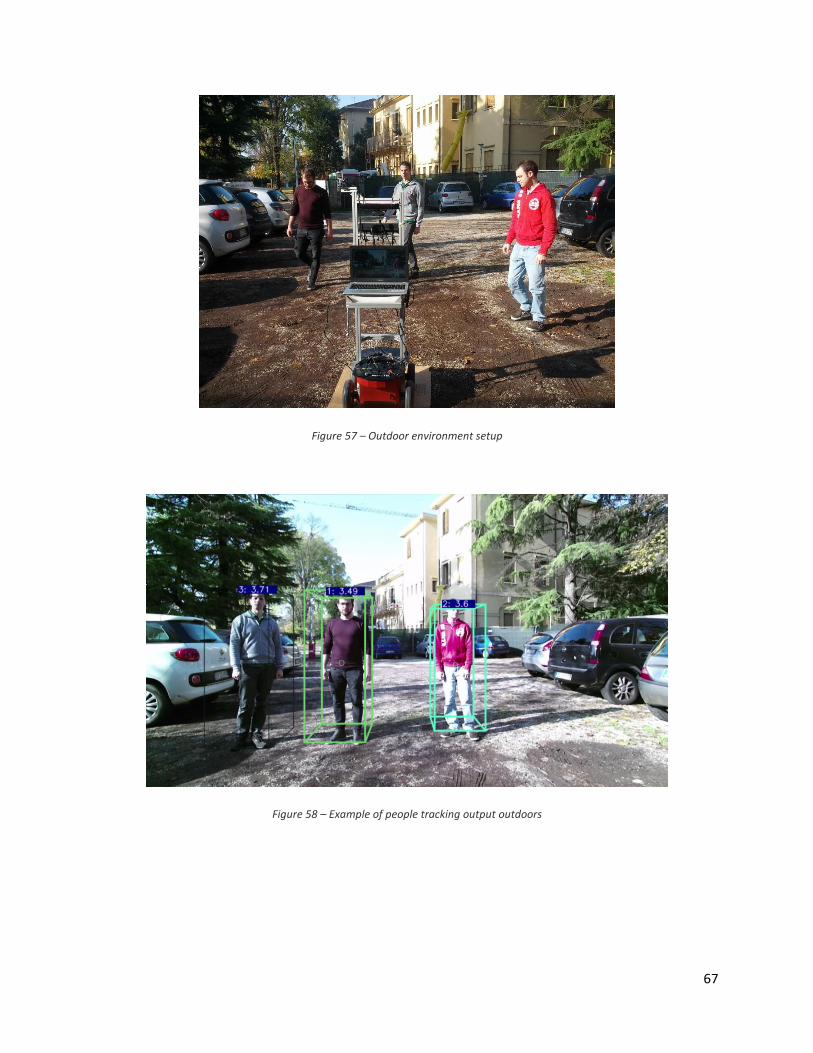
67

Figure 57 – Outdoor environment setup

Figure 58 – Example of people tracking output outdoors

68

Figure 59 – Example of people tracking outdoors. On the left: the tracker output. On the right: the Kinect One’s point cloud.

4.1.5 Results

The outdoor test proved that the new Kinect is able to track people in an outdoor environment. Figure 58

shows the tracking results outdoors; the people in the scene were illuminated by the sun, but the Kinect

was capable to recognize them. The point clouds acquired in that type of scene is not as good as in an

indoor environment, as showed in Figure 59, but it is enough to make the tracker works.

From this experiment, we could appreciate the advantage of using ROS as a robotic framework and, in

particular, of software modularity. If a package is well developed, as in this case, it is straightforward to

adapt it to new tools or sensors. For people tracking and following applications, it is not easy to define a

clear winner between Kinect 360 and v2 because both offer advantages: the first generation is

computationally lighter, while the second generation allows an outdoor use and at longer distances. If the

fluidity and responsiveness of the system is a key feature, then, the best choice is the Kinect 360, which

guarantees, with a PC with average performance, to reach 30 fps. The computational weight of the new

Kinect, due to the higher resolution of the sensors, is such that pledges only 5 fps in a high-end PC and

this involves a less responsive system and less fluidity in movements. However, if the precision in the

metric estimation of people positions matters, as in multi-camera scenarios, or if tracking has to be done

outdoors, then the best choice is the new Kinect.

69

4.2 PEOPLE TRACKING SCORES

In the previous test, we showed the better results of the Kinect One in outdoor, now we quantitatively

test the performance of the Kinects and compare the results.

4.2.1 Setup

To evaluate the tracking performance we used the evaluation procedure described in [5]. The MOTA index

gives an idea of the number of errors that are made by the tracking algorithm in terms of false negatives,

false positives and mismatches, while the MOTP indicator measures how well exact positions of people

are estimated. The higher these indices are, the better is the tracking performance. Other than the MOTP

and MOTA indices, we report also the false positive and false negative percentages and the total number

of identity (ID) switches, which represents the number of times tracks change ID over time.

We collected three ROS bag10 of different situations: in the first scene, seven people randomly walked

around (as showed in Figure 60), in the second, two persons walked from near range to far (as showed in

Figure 61) and, in the last, two persons walked behind some tables at different distances (as showed in

Figure 62).

Figure 60 – Example of the first scene

10 http://wiki.ros.org/rosbag

70

Figure 61 – Example of the second scene

Figure 62 – Example of the third scene

4.2.2 Results

Table 8 shows the results with the first scene; MOTP value is sometimes better with the Kinect 360 but

the other values indicate that the Kinect One works better. In the scene, there was a lot of people, thus

the ID switches are high but ID switches score obtained with the Kinect One are less than half of Kinect

360. So, if both work well, the new Kinect performs better. In the second scene, the Kinect 360 was not

able to track well the persons when far away (about 9.5 m) and this is showed in Table 9; in particular, the

high false negative value of Kinect 360 is interesting. In the same scene, the Kinect One performed well

and correctly tracked the persons in all positions; this confirms all the previous tests. In the end, we see

from Table 10 that Kinect One worked better in the third scene as well. The high FN value of the Kinect

360 is due to the person in the far field, the Kinect did not see him. In all the scene, the MOTP index

indicates that both Kinects correctly estimated the people position, but the MOTA highlights that the

Kinect 360 makes more mistakes, thus we can say that Kinect One works better for people tracking

applications.

71

Kinect 360 Kinect One

MOTP 73.04% 77.7582%

MOTA 36.8379% 59.7621%

FP% 9.6576% 9.5144%

FN% 52.5147% 30.3271%

ID switches 37 16

Table 8 – Results for the first scene

Kinect 360 Kinect One

MOTP 72.653% 68.0967%

MOTA 41.954% 81.25%

FP% 6.9787% 0.6068%

FN% 50.821% 18.1432%

ID switches 3 0

Table 9 – Results for the second scene

Kinect 360 Kinect One

MOTP 74.7277% 72.5947%

MOTA 2.0421% 47.4522%

FP% 1.9183% 5.2866%

FN% 95.9158% 47.0701%

ID switches 2 3

Table 10 – Results for the third scene

72

5 CONCLUSIONS

This thesis can be subdivided into three sections: in the first, we worked with Kinect SDK to extract the

data, in the second, we used those data to compare the Kinects and, in the last part, we use Kinect’s data

in real robotics and computer vision applications. In the first part, we studied and compared the Kinect’s

technologies and the available SDKs. We created a program that records all the Kinect data and this

teached us how to save a lot of data, in real-time, without losing any information. The techniques used

and the solutions found can be useful for many other works.

In the second part, we showed how to perform some test starting from the test setup and ending to the

results analysis. In all the tests, the Kinect One performs better showing the great work made.

In the last part, the robotic application confirmed the previous results and highlighted, another time, the

Kinect One superiority.

Thus, to conclude, we summarize the main Kinects features

Kinect One features:

Point clouds created are very precise, really better then Kinect 360;

It is almost immune to artificial light variation;

It works outdoors, also with scene in sun;

It has a good depth accuracy and works until 10 m;

It works well for people tracking applications.

Kinect 360 features:

Computationally lighter than the Kinect One, thus the best choice for indoor people following

and with low end computer.

73

REFERENCES

[1] K. Khoshelham, “Accuracy Analysis of Kinect Depth Data,” International Archives of the

Photogrammetry, Remote Sensing and Spatial Information Sciences, 2011.

[2] J. Sell and P. O’Connor, “The XBOX One System on a Chip and Kinect Sensor,” Micro, IEEE, vol. 34,

no. 2, pp. 44-53, March 2014.

[3] M. Munaro, A. Basso, A. Fossati, L. V. Gool and E. Menegatti, "3D Reconstruction of Freely Moving

Persons for Re-Identification with a Depth Sensor," in International Conference on Robotics and

Automation (ICRA), 2014.

[4] "Distances Computation," 22 September 2012. [Online]. Available:

http://www.cloudcompare.org/doc/wiki/index.php?title=Distances_Computation. [Accessed

November 2014].

[5] M. Munaro and E. Menegatti, “Fast RGB-D People Tracking for Service Robots,” in Autonomous

Robots (AURO), 2014.

[6] Microsoft Corporation, “Kinect for Windows features,” 01 09 2014. [Online]. Available:

http://www.microsoft.com/en-us/kinectforwindows/meetkinect/features.aspx.

[7] Microsoft Corporation, “Using Kinect Body Tracking,” 01 09 2014. [Online]. Available:

http://msdn.microsoft.com/en-us/library/dn772820.aspx.

[8] M. Bonanni, “Kinect V2: body source – joints,” 17 03 2014. [Online]. Available:

http://codetailor.blogspot.it/2014/03/kinect-v2-body-source-joints.html.

[9] F. Dai, “The New (Time-of-Flight) Kinect Sensor and Speculations,” 22 5 2013. [Online]. Available:

http://blog.falcondai.com/2013/05/the-new-time-of-flight-kinect-sensor.html.

[10] T. Kerkhove, “First look at Expressions – Displaying expressions for a tracked person,” 13 07 2014.

[Online]. Available: http://www.kinectingforwindows.com/2014/07/13/first-look-at-expressions-

displaying-expressions-for-a-tracked-person/.

74

[11] N. Smolyanskiy, “High Precision Face Tracking and Face Modelling in XBox One Kinect,” 14 02 2014.

[Online]. Available: http://nsmoly.wordpress.com/2014/02/14/high-precision-face-tracking-and-

face-modelling-in-xbox-one-kinect/.

[12] Wikipedia, “Time-of-flight camera,” 01 09 2014. [Online]. Available:

http://en.wikipedia.org/wiki/Time-of-flight_camera.

[13] "libfreenect2," 2014. [Online]. Available: https://github.com/OpenKinect/libfreenect2.

[14] "Cloud Compare," 2014. [Online]. Available: http://www.danielgm.net/cc/.

[15] "ROS," 1 12 2014. [Online]. Available: http://www.ros.org/.

[16] “Accuracy and precision,” [Online]. Available:

http://en.wikipedia.org/wiki/Accuracy_and_precision. [Accessed November 2014].

[17] M. M., F. Basso, M. S., P. E. and M. E., “A Software Architecture for RGB-D People Tracking Based

on ROS Framework for a Mobile Robot,” in Frontiers of Intelligent Autonomous Systems, Springer,

2013, pp. 53-68.