Embed Size (px)
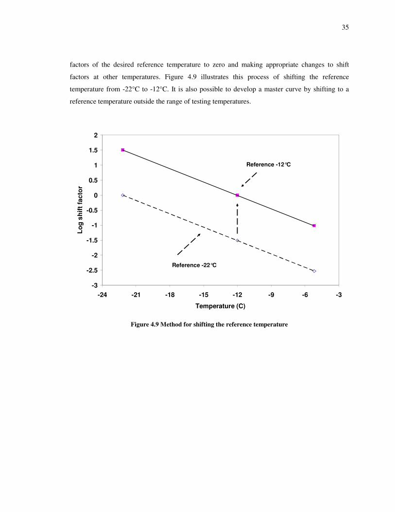
Citation preview

The Pennsylvania State University
The Graduate School
Department of Civil and Environmental Engineering
Evaluation of Low Temperature Properties of SISSI Mixtures
and Binders
A Thesis in
Civil Engineering
by
Laxmikanth Premkumar
2008 Laxmikanth Premkumar
Submitted in Partial Fulfillment of the Requirements
for the Degree of
Master of Science
December 2008
The thesis of Laxmikanth Premkumar was reviewed and approved* by the following:
Ghassan R. Chehab Assistant Professor of Civil and Environmental Engineering Thesis Co-Advisor
Mansour Solaimanian Senior Research Associate, The Thomas D. Larson Pennsylvania Transportation Institute Thesis Co-Advisor
Shelley M. Stoffels Associate Professor of Civil and Environmental Engineering
Peggy A. Johnson Professor of Civil and Environmental Engineering Head of the Department of Civil and Environmental Engineering
*Signatures are on file in the Graduate School

iii
ABSTRACT
The main objective of this thesis is to revisit and build on the equivalence principle that
governs the low temperature Superpave™ binder specifications. Bending beam rheometer (BBR)
tests were conducted on asphalt binders from wearing layers of seven Superpave In-situ Stress
Strain Investigation (SISSI) project sites. All the asphalt binders were aged with pressure aging
vessel (PAV) prior to conducting the BBR tests. Both 240 second and 2 hour tests were
conducted at three different temperatures, at the low temperature of the asphalt PG grade, 10°C
higher than the lower temperature grade and at -5°C to obtain the flexural creep stiffness [S(t)]
master curves. Additionally, indirect tensile tests (IDT), to capture the low temperature properties
of the mixtures, were conducted on field mixtures obtained from the wearing layers of all the
SISSI sites.
From the BBR test results, it is observed that the equivalence principle that governs the
low temperature Superpave™ binder specification does not hold for the SISSI binders tested and
therefore alternate times and temperatures for testing are suggested in this research to deliver an
equivalent stiffness. However, further testing on other types of asphalt binders is required to reach
a comprehensive consensus.
Further, the time-temperature shift factors for the SISSI binders are compared with the
Strategic Highway Research Program (SHRP) and SISSI mixtures. The SISSI and SHRP shift
factor curves do not match, contradicting the fact that all asphalt binders can be characterized by
similar shift factors. The shift factors of the SISSI binders and mixtures tend to match well at
higher than at lower testing temperatures. Finally, all the SISSI sites are ranked in accordance
with their low temperature asphalt binder and mixture properties and the results are presented.

iv
TABLE OF CONTENTS
List of Figures………………………………………………………………………….....vii
List of Tables……………………………………………………………………………...xii
Acknowledgements………………………………………………………………............xiii
1. Introduction…………………………..………………………………………………..1
1.1. Background………………………………………………………………………....1
1.2. Problem Statement……………………………………………………………….....2
1.3. Research Objectives and Significance……………………………………………...2
1.4. Research Approach………………………………………………………………....3
2. Review of Literature...…………………………………………..................................5
2.1. Thermal Cracking in Asphalt Pavements…………………………………………..5
2.2. Indirect Tensile Test (IDT)........................................................................................6
2.3. The Bending Beam Rheometer (BBR)………………………………………….....11
3. SISSI Project……………………………………………………………………….....17
3.1 Background ……………………………………………………………………......17
3.2 Site Selection……………………………………………………………………....18
3.3 Pavement Construction………………………………………………………….....19
3.4 Pavement Instrumentation………………………………………………………....21
3.5 Material Characterization……………………………………………………….....23
3.5.1 Binder Characterization…………………………………………………………....23
3.5.2 Mixture Characterization………………………………………………………......23

v
4. Viscoelastic Material Characterization…………………………………………….25
4.1. Introduction……………………………………………………………………....25
4.2. Linear Viscoelastic Unit Response Functions……………….…………………...27
4.2.1. Complex Modulus (E*)…………………………………………...……………...27
4.2.2. Creep Compliance D(t)…………………………………………………………..29
4.3. Flexural Creep Stiffness and m-value……………………………………………30
4.4. Construction of Master curve using Time - Temperature Superposition………...31
5. Test Methods, Equipment and Testing Protocol………………………………….37
5.1. Test Equipment and Instrumentation……...…………………………….……….37
5.2. Test Methods and Protocol……………...………………………………………..41
5.2.1. Materials and Mixtures used……………………………………..…………….....41
5.2.1.1 Determining the IDT Specimen Dimensions and Air void Content……………..43
5.2.1.2 Superpave Performance-Grading (PG) System....................………….................44
5.2.2. IDT Testing Program for Asphalt Mixtures ........................………………….…46
5.2.3. BBR Testing Program…………………………………………………………...48
6. Results and Analysis……………..…………………………………………………53
6.1 D(t) and Tensile Strength of SISSI Mixtures………………………………….....53
6.2 S(t) and m-value of SISSI Binders……………………………………………….58
6.3 Comparison of IDT and BBR Shift Factor Functions…………………………....71
6.4 Relationship Between Low Temperature Properties of SISSI Mixtures
and Binders……………………………………………………………………....76
6.5 Ranking of SISSI Sites Based on IDT and BBR Material Properties………..….78
7. Conclusions and Recommendations…………………....……………………….…82
7.1. Conclusions……………………………………………………..…………..........82

vi
7.2. Recommendations for FutureWork........................………..........................……83
References...……………………………………………………………………..…........84
Appendix A …………………………..…………………………………………………88
Appendix B …………………………..………………………………………………..105
Appendix C.……………………………………………………………………………119

vii
LIST OF FIGURES
Figure 1.1: Methodology Flowchart………………………………………………................4
Figure 2.1: Top view of thermal cracking in flexible pavements…………………………...5
Figure 2.2: Elastic stress distribution in an IDT specimen………………………………….6
Figure 2.3: Typical stress states in asphalt concrete layers with loading…………………...7
Figure 2.4: Direction of crack in an IDT specimen………………………………………....7
Figure 2.5: Precision for compliance for six laboratories…………………………………..10 Figure 2.6: D2s precision for Poisson’s ratio for six laboratories…......................................10 Figure 2.7: Specimen geometry for BBR test……………………………………………....12 Figure 2.8: Time-Temperature shift factors for SHRP asphalt binders…………………….14 Figure 2.9: Schematic of the BBR………………………………………………………….15 Figure 3.1: SISSI test sites………………………………………………………………….18 Figure 3.2: Load associated transducers……………………………………………………22 Figure 3.3: Resistivity probe for frost depth and time domain reflectometer for moisture
content sensors………………………………………………………………..22 Figure 4.1: Strain responses to a static load input (a); (b) elastic, (c) viscous, (d) viscoelastic………………………………………………………………....25 Figure 4.2: Sinusoidal stress and strain response……………………………………..........28 Figure 4.3: Complex modulus decomposed into real and imaginary components…............29 Figure 4.4: Typical load vs. vertical deformation plot for an IDT test………………..........30 Figure 4.5: Flexural creep stiffness vs. time curves for a typical BBR test…………...........33 Figure 4.6: Flexural creep stiffness master curve at reference temperature of -12°C...........33 Figure 4.7: Log shift factor vs. temperature for the BBR test………………………...........34
Figure 4.8: Flexural creep stiffness master curve at reference temperatures of -12°C and 22°C………………………………………………………………..34

viii
Figure 4.9: Method for shifting the reference temperature…...............................................35
Figure 5.1: Complete setup of the MTS and Partlow controller………….………..............38 Figure 5.2: IDT test setup….................................................................................................38 Figure 5.3: Complete setup of the BBR…………………………………………………....40 Figure 5.4: BBR test specimen between supports……………………………………….....40 Figure 5.5: Steps involved in preparing a BBR specimen; (a) mould preparation, (b)
pouring the asphalt binder, (c) trimming the surface, (d) sample specimen……....................................................................................................42
Figure 5.6: Distribution of air void content (%) in gyratory compacted specimens……....43 Figure 5.7: Relation of the Superpave™ binder tests to performance………….................46 Figure 5.8: LVDT setup on the IDT specimen……………................................................47 Figure 5.9: Check for LVE conditions……………………………………………….........50 Figure 5.10: Loading curve before and after installation of needle valve..............................51 Figure 5.11: BBR testing protocol for one test temperature..................................................52 Figure 6.1: Creep compliance vs. time for replicates of Mercer East in semi-log domain ..............................................................................................................54 Figure 6.2: Creep compliance vs. reduced time for replicates of Mercer East in semi-log
domain...............................................................................................................55 Figure 6.3: Extended sigmoidal fit for replicates of Mercer East in semi-log domain........55 Figure 6.4: Shift factor curve for replicates of Mercer East................................................56 Figure 6.5: Creep compliance master curves for all SISSI sites at reference temperature of -10°C..............................................................................................................57 Figure 6.6: Average tensile strength values for all SISSI sites............................................57 Figure 6.7: Flexural creep stiffness vs. time for Somerset on a semi-log scale...................58 Figure 6.8: Flexural creep stiffness vs. reduced time for Somerset on a semi-log scale.....59 Figure 6.9: Shift factor curves for Somerset on a semi-log scale........................................59 Figure 6.10: Comparison of average S(60) at T1+10 for SISSI sites....................................60

ix
Figure 6.11: Comparison of m(60) at T1+10 for SISSI sites .................................................61 Figure 6.12: Comparison of m(60) at T1+10 for 240s and 2hr BBR tests for Somerset .......62 Figure 6.13: Average % difference between S(60) @ T1 +10 and S(7200) @ T2 ................65 Figure 6.14: Average predicted time for S(60) @ T1 +10 and S(7200) @ T2 to be equivalent .........................................................................................................65 Figure 6.15: Predicted temperature for S(60) @ T1 +10 and S(7200) @ T2 to be equivalent .........................................................................................................66 Figure 6.16: Comparison of shift factors for SHRP core asphalts and SISSI binders ..........69 Figure 6.17: Predicted S(60) at -22°C and -5°C for SHRP and SISSI asphalt binders ........70 Figure 6.18: Average shift factors obtained from IDT and BBR tests .................................71 Figure 6.19: (a) Parallel D(t) curves at low temperatures,(b) D(t) master curve with log
shift factor of 1.9 @ -22°C ...............................................................................72 Figure 6.20: D(t) master curve with log shift factor of 1.6 @ -22°C ....................................73 Figure 6.21: (a) D(t) master curve with log shift factor of 1.5 @ -22°C(b) D(t) master curve
with log shift factor of 1.3 @ -22°C ................................................................74 Figure 6.22: Comparison of average creep compliance/stiffness data for SISSI mixtures and
binders ..............................................................................................................76 Figure 6.23: Comparison of average m-value for SISSI mixtures and binders ....................77 Figure 6.24: Tensile strength and thermal stress obtained from BBR and DT testing .........79 Figure 6.25: Thermal cracking in Delaware section .............................................................80 Figure A1: Creep compliance vs. time (a) and creep compliance master curve (b) for Blair ............................................................................................................88 Figure A2: Shift factor curve (a) and creep compliance master curve at -10°C (b) for Blair ............................................................................................................89 Figure A3: Creep compliance vs. time (a) and creep compliance master curve (b) for Delaware .................................................................................................... 90 Figure A4: Shift factor curve (a) and creep compliance master curve at -10°C (b) for Delaware .....................................................................................................91

x
Figure A5: Creep compliance vs. time (a) and creep compliance master curve (b) for Mercer East .................................................................................................92 Figure A6: Shift factor curve (a) and creep compliance master curve at -10°C (b) for Mercer East .................................................................................................93 Figure A7: Creep compliance vs. time (a) and creep compliance master curve (b) for Mercer West................................................................................................94 Figure A8: Shift factor curve (a) and creep compliance master curve at -10°C (b) for Mercer West................................................................................................95 Figure A9: Creep compliance vs. time (a) and creep compliance master curve (b) For Perry ..........................................................................................................96 Figure A10: Shift factor curve (a) and creep compliance master curve at -10°C (b) for Perry ..........................................................................................................97 Figure A11: Creep compliance vs. time (a) and creep compliance master curve (b) for Somerset .....................................................................................................98 Figure A12: Shift factor curve (a) and creep compliance master curve at -10°C (b) for Somerset......................................................................................................99 Figure A13: Creep compliance vs. time (a) and creep compliance master curve (b) for Tioga..........................................................................................................100 Figure A14: Shift factor curve (a) and creep compliance master curve at -10°C (b) for Tioga..........................................................................................................101 Figure A15: Creep compliance vs. time (a) and creep compliance master curve (b) for Warren ......................................................................................................102 Figure A16: Shift factor curve (a) and creep compliance master curve at -10°C (b) for Warren ......................................................................................................103 Figure B1: Creep stiffness vs. time (a) and creep stiffness master curve (b) for Blair .....105 Figure B2: B2 Shift factor curve for Blair ........................................................................106 Figure B3: Creep stiffness vs. time (a) and creep stiffness master curve (b) for Delaware .........................................................................................................107 Figure B4: B2 Shift factor curve for Delaware .................................................................108

xi
Figure B5: Creep stiffness vs. time (a) and creep stiffness master curve (b) for Mercer East .....................................................................................................109 Figure B6: B2 Shift factor curve for Mercer East..............................................................110 Figure B7: Creep stiffness vs. time (a) and creep stiffness master curve (b) for Mercer West ....................................................................................................111 Figure B8: B2 Shift factor curve for Mercer West ............................................................112 Figure B9: Creep stiffness vs. time (a) and creep stiffness master curve (b) for Perry .....113 Figure B10: B2 Shift factor curve for Perry ........................................................................114 Figure B11: Creep stiffness vs. time (a) and creep stiffness master curve (b) for Somerset ..........................................................................................................115 Figure B12: B2 Shift factor curve for Somerset ..................................................................116 Figure B13: Creep stiffness vs. time (a) and creep stiffness master curve (b) for Warren ............................................................................................................117 Figure B12: B2 Shift factor curve for Warren .....................................................................118

xii
LIST OF TABLES
Table 2.1: Coefficients to calculate the creep compliance and Poisson’s ratio .....................9 Table 2.2: Temperature shift factors for SHRP asphalt binders ..........................................13 Table 3.1: Highways selected for instrumentation ...............................................................19 Table 3.2: Construction information for SISSI sites ............................................................20 Table 3.3: Performance grade binders used at SISSI sites ...................................................21 Table 3.4: Summary of testing programs followed for the SISSI procured asphalt mixes ..24 Table 5.1: Compaction temperature (°C) and Gmm for wearing layers of SISSI sites .........41 Table 5.2: Superpave™ binder test equipment ....................................................................45 Table 6.1: Air void content (%) and number of replicates for SISSI - IDT specimens .......53 Table 6.2: Sigmoidal coefficients for Mercer East ..............................................................56 Table 6.3: Hyperbolic fit coefficients ..................................................................................60 Table 6.4: Actual and predicted flexural creep stiffness values (MPa) for SISSI binders ..64 Table 6.5: % Difference, actual time and temperature predicted for SISSI sites ................67 Table 6.6: % Slope and R2 for shift factor curves for binders from the SISSI sites ............68 Table 6.7: Predicted S(60) for SHRP and SISSI asphalt binders ........................................69 Table 6.8: Hyperbolic fit coefficients ..................................................................................70 Table 6.9: Shift factor values for D(t) and S(t) master curves .............................................75 Table 6.10: Ranking of SISSI sites based on IDT and BBR test results ................................80 Table 6.11: Ranking of all SISSI sites based on IDT test results ...........................................81 Table A1: Sigmoidal coefficients for the SISSI sites .........................................................104 Table C1: M-values for 240s and 2hr BBR tests on SISSI binders ...................................119

xiii
ACKNOWLEDGEMENTS
First of all, I would like to express my sincere gratitude to my parents, relatives and my grandma
for trusting my judgment to pursue a Master’s in the United States. I also thank my BITS
professors, Dr. Rao and Dr. Sandra for showing me the road to pavement engineering.
None of this would be possible without the patient guidance and encouragement of my research
advisor Dr. Ghassan Chehab throughout the course of my study. I also thank him for being a
friend, philosopher and guide and for bringing out the best in me.
I am also greatly indebted to my co-advisor, Dr. Mansour Solaimanian for providing me with
financial support along with continued guidance during the course of my study at Penn State. I
also thank Dr. Shelley Stoffels, for her support and for reviewing this thesis and providing
invaluable suggestions. I will also miss her classes, which were both indulging and informative.
Thanks to my fellow students Carlos, Dr. Hao, Tang, Tanmay, Marcelo and Scott for being there
equally during good and tough times. Special thanks to Dan, Deno, Joe, Tom and others who
helped me fix machines in time of need.
Last but not the least, I thank all my friends Prashant, Jag, Praks, Ananth, VJ, Santh, Gir and all
members of F16 for providing me with great company and making me always feel at home.

1
1. INTRODUCTION
1.1 BACKGROUND
Asphalt pavements form a major component of the highway infrastructure and are essential for
the movement of people and goods. Pavement surfaces, being part of the highway, also affect the
cost, ride quality and safety of the users. As the highway infrastructure plays an important part in
the economic growth of a country, good quality and long lasting pavements are necessary. The
Strategic Highway research program (SHRP) was established in 1987 as a five year research
program to improve the performance and durability of the United States roads. A major outcome
of the SHRP project was Superior Performing Asphalt Pavements (Superpave™) mix design and
Performance Grade (PG) binder systems. The Superpave™ system incorporates performance
based testing on asphalt binders and mixtures to control rutting, low temperature cracking and
fatigue cracking in asphalt pavements, i.e. the tests and analysis has a direct relationship with
field performance (Asphalt Institute, 1996).
Performance graded binders are defined by a term, for example PG 64-22. The first number, in
degrees Celsius, is the high temperature grade which corresponds to the high pavement
temperature the binder is expected to serve. Similarly, the second number in the PG binder, -22, is
the low temperature grade or the low temperature up to which the binder possesses adequate
physical properties. The Superpave™ binder specification is unique as the testing temperatures
are varied, while the criteria for material property remain the same. This is because, for example,
though good performance of asphalt binders is required in both Texas and Pennsylvania; different
types of binders will be required due to different climatic conditions.
One of the principal modes of failures in asphalt concrete pavements is low temperature thermal
cracking and it depends on both the properties of the asphalt mixtures and binders. Typically,
thermal cracking in asphalt pavements occurs when the thermal stresses developed in the
pavements exceed its tensile strength. Though the properties of the mixture as a whole are
important, the asphalt binder with its ability to absorb the stresses plays a pivotal role in
preventing thermal cracking.
In Superpave™ specification, the Bending Beam Rheometer (BBR) and Direct tension (DT) tests
are tests used to characterize the low temperature properties of the asphalt binder. The critical
cracking temperature, i.e. the expected temperature of cracking in the field can be obtained by

2
plotting the thermal stresses and tensile strength values calculated from the BBR and DT
respectively. The temperature at which the thermal stress exceeds the strength represents the
critical cracking temperature. Similarly, the TC model developed as a part of the SHRP A-005
program can be used to predict the thermal cracking versus time for asphalt pavement structures
using material properties from the Indirect Tensile Test (IDT) on asphalt mixtures. Thus, low
temperature properties of asphalt binders and mixtures obtained from laboratory testing play an
important role in predicting the low temperature performance of pavements in the field.
1.2 PROBLEM STATEMENT
Thermal cracking is one of the most prominent distresses in asphalt concrete pavements and is
usually oriented in a direction transverse to the traffic. Thermal cracking typically occurs when
the thermal stresses developed in the pavement exceed its strength and is augmented by thermal
cooling cycles or traffic. Various factors like rate of cooling of pavement temperature, pavement
and subgrade type, traffic and climatic conditions tend to affect the occurrence of thermal
cracking (Bahia 1991, Buttlar 1996). But the properties of the mixture and binder tend to form the
crux for low temperature cracking. Hence studying the low temperature properties of the asphalt
binders and mixtures will aid in establishing the performance of the pavement structure at lower
service temperatures.
1.3 RESEARCH OBJECTIVES AND SIGNIFICANCE
IDT and BBR are two tests conducted on asphalt concrete mixtures and asphalt binders
respectively to capture the low temperature properties. The American Association of State
Highway and Transportation Officials (AASHTO) procedures for the IDT test provide elastic
solutions to determine the low temperature creep compliance of the mixtures. However,
viscoelastic solutions for the same are available (Wen 2001) and are used in this study for
analysis.
BBR test procedures developed in the 1990s specify that the flexural creep stiffness [S(t)] should
not exceed 300MPa at exactly 60 seconds of the 240 second creep test at 10°C above the
minimum service temperature. Though several loading times ranging from 300 seconds to 20,000
seconds were used by researchers in the past, a loading time of 240 seconds was considered
practical for testing purposes. This was concluded through comprehensive studies conducted
while developing the BBR. It was also found that the slope of the shift factor curve obtained
while developing the S(t) master curve was very similar for all asphalt binders and was within the

3
range of 0.173 log(s)/° C and 0.199 log(s)/°C. However these specifications were developed prior
to the Superpave™ design procedures. With Superpave™ binder grades developed, it is pertinent
to check if all binders still exhibit the same shift factor curve and to revisit and build on the
equivalence principle that the S(t) at 7200 seconds at the lower temperature grade is equivalent to
S(t) at 60 seconds at 10°C above the lower temperature grade. This research could serve as a
foundation for establishing changes to the current BBR protocol.
1.4 RESEARCH APPROACH
The research presented here was conducted as part of a Pennsylvania Department of
Transportation (PennDOT) project titled ‘Superpave In-Situ Stress/Strain Investigation (SISSI).’
To meet the study objectives, a literature review on the current BBR Superpave™ specifications
and IDT testing was first conducted. The experimental work began with testing SISSI asphalt
mixtures to obtain creep compliance [D(t)] and tensile strength in the IDT mode. The results
obtained from these tests were later used to rank the SISSI sites. BBR tests at different
temperatures and times were conducted on seven PAV aged SISSI binders to obtain the S(t)
master curves. The BBR test results are utilized to evaluate the equivalence principle governing
the BBR test specifications. The shift factors obtained from the BBR master curves are compared
with the IDT and SHRP shift factors. The SISSI sites are then ranked for thermal cracking
susceptibility based on the material properties obtained from asphalt mixture and binder test
results. The methodology adopted in this thesis is shown in the form of a flowchart in Figure 1.1.

4
Figure 1.1 Methodology flowchart
BBR
Creep
Compliance m value Stiffness master
curve for 240s test
Stiffness master curve
for 2 hr test
Evaluate the equivalence
principle
SHRP asphalts shift
factors
Tensile Strength
Rank SISSI sites
mixture binder
Shift Factor Shift Factor
compare
IDT
SISSI

5
2. REVIEW OF LITERATURE
2.1 THERMAL CRACKING IN ASPHALT PAVEMENTS
Low temperature cracking or thermal cracking occurs in asphalt pavements when the tensile
stresses developed exceed its strength. This results in cracks transverse or perpendicular to the
direction of the traffic which are usually equally spaced (Jung et al., 1992). Thermal cracking
primarily occurs due to temperature variations and is augmented by traffic loading. Thus, the top
layer or the wearing layer of the pavement structure, which is exposed to greater temperature
variations than the underlying layers, is usually more susceptible to thermal cracking (OECD,
2005).
Thermal cracks permit the migration of water and fines into the pavement structure causing local
settlement of the pavement. The water entering through these cracks form ice lenses which can
lead to the formation of cavities that eventually collapse under heavy vehicular loads. Thus
control of thermal cracking is essential for design of good quality flexible pavements (Buttlar,
1996).
Several factors influence thermal cracking in asphalt pavements which include material type,
pavement structure, rate of cooling of the pavement structure and temperature (Jung et al., 1992).
However to control thermal cracking, the low temperature properties of the asphalt mixture and
binder are properties that can be modified effectively by the designer. The top view of thermal
cracking in pavement structure is shown in Figure 2.1.
Figure 2.1 Top view of thermal cracking in flexible pavements
Traffic

6
2.2 INDIRECT TENSILE TEST (IDT)
Thermal stresses developed in the pavements are the primary cause for thermal cracking in
asphalt pavements. Also the fracture property of the mixture is important as it determines the
amount of cracking that will develop when subjected to thermal stresses (SHRP-357). Hence it is
important to measure the thermal stress and fracture properties of the asphalt mixture to
understand its low temperature behavior. Thermal stresses can be derived from relaxation
modulus of a mixture. However, the relaxation modulus, which requires a constant strain, is
practically difficult to conduct. Hence creep tests were selected as they could be conducted in
either direct or indirect tension mode.
The vertical and horizontal stress distribution for a 100mm x 38mm (diameter x height) asphalt
concrete specimen used in IDT tests is shown in Figure 2.2. It can be observed that the stress
distribution, near the center of the specimen is uniform. The stresses in this zone are also
unaffected by the end effects near the loading strips. Thus deformation measurements near the
center of the face of the specimen are not significantly influenced by stress concentrations near
the loading strips (SHRP -357).
Figure 2.2 Elastic stress distributions in an IDT specimen. (Wen, 2001)
Typically, cracking due to loading in asphalt pavements initiates at the bottom of the asphalt
layer, under the wheel load, with horizontal tensile stresses occurring at the bottom and
compressive stresses at the top as shown in Figure 2.3. It is also to be noted that the stress state in
the center of an IDT specimen is very similar to that occurring in the bottom of asphalt

7
pavements. Additionally as shown in Figure 2.4, in the IDT mode, cracking occurs in the
direction perpendicular to loading, unlike uniaxial tests, thereby depicting field conditions.
Figure 2.3 Typical stress states in asphalt concrete layers with loading (Kumar, 2006)
Figure 2.4 Direction of crack in an IDT specimen
The IDT creep and tensile strength tests were developed as part of the Strategic Highway
Research Program. A measurement and analysis system to determine the creep compliance and
tensile strength in the IDT mode was developed by Roque and Butler (1992) and is incorporated
in ASSHTO TP9-96, Standard Test Method for Determining the Creep Compliance and Strength
of Hot Mix Asphalt (HMA) Using the Indirect Tensile Test Device. A new gage-point
measurement system was developed through Roque’s study and the measured vertical and
horizontal deformations are used to calculate the Poisson’s ratio, rather than assuming a constant
value of 0.35. The aggregate size effect, stress distribution in the specimen area and bulging
effects were considered in the design of the mounting system used and positioning of LVDTs on
the specimen surface. Based on finite element analysis, gage lengths of 1-in and 1.5-in for
100mm and 150mm specimens were recommended. The elastic solutions for determining the
Load

8
creep compliance and Poisson’s ratio of asphalt mixtures tested in the IDT mode is shown in
Equations 2.1 and 2.2:
( ) CGLP
bDXtD ×
×
××=
2.1
where,
D(t) = creep compliance,
X = average, normalized horizontal deformation at 50 seconds,
D = diameter of specimen,
b = thickness of specimen,
P = load applied,
GL = gauge length, and
C = correction factor for bulging.
222
778.048.11.0
−
+−=
Y
X
D
b
Y
Xν
2.2
where,
υ is the Poisson’s ratio,
X is the horizontal deformation, and
Y is the vertical deformation.
However as asphalt is viscoelastic in nature, viscoelastic solutions to determine the creep
compliance and Poisson’s ratio were developed by Wen (2001) as shown in Equation 2.3.
( ) ( ){ }
)()(
)()(
)(
22
11
tVbtUa
tVbtUa
teVtcUP
dtD
+
+−=
+−=
υ
2.3

9
where,
d is specimen thickness,
P is load applied to specimen in indirect tension mode,
U(t) is horizontal deformation of specimen,
V(t) is vertical deformation of specimen,
υ is Poisson’s ratio, and
c, e, a1, a2 , b1 and b2 are coefficients.
For a 100mm diameter specimen and gage length of 25.4 mm, the coefficients developed by Wen
(2001) are shown in Table 2.1.
Table 2.1 Coefficients to calculate the creep compliance and Poisson’s ratio
Coefficient Value
c 0.7874
e 2.2783
a1 3.385
a2 1.081
b1 1.000
b2 3.122
The tensile strength of the mixture is important in determining its fracture properties and is also
included in the theory of crack growth of non-linear viscoelastic materials developed by Schapery
(1984). The tensile strength test is conducted at -10°C where the specimen is failed under a
constant crosshead rate. It is observed that micro cracks tend to form even before the specimen
fails. For obtaining the fracture parameters, it is more important to know the true load for failure
than the maximum. The true point of failure is defined as occurring when the difference between
the vertical and horizontal deformations reaches a maximum which can be determined by using
LVDT measurements. However, it was found that using LVDTs for strength tests resulted in
damage or destruction of the transducers (NCHRP 530). Hence, it is recommended that LVDTs
not be used during the strength test and that the uncorrected strength is adjusted using the
empirical relationship shown in Equation 2.4 (NCHRP 530).
Tensile Strength = 0.25 + (0.78* IDT strength) MPa 2.4

10
The precision evaluation of the IDT tests was conducted as part of Phase III of NCHRP Project 9-
29, which assessed the AASHTO T322 method. IDT test data from six laboratories was used in
this evaluation. The d2s precision or the maximum allowable difference between two samples for
95% of the time was calculated, and it was observed that the variability in D(t) was as high as 10-
30%. For single operator precision, the average d2s for all laboratories was 22, 28 and 32 percent
at the lowest, intermediate and high temperatures of testing, respectively. Figures 2.5 and 2.6
represent the d2s precision values for D(t) and Poisson’s ratio.
Figure 2.5 D2s Precision for compliance for six laboratories (NCHRP 530)
Figure 2.6 D2s Precision for Poisson’s ratio for six laboratories (NCHRP 530)

11
2.3 THE BENDING BEAM RHEOMETER (BBR)
The relationship between asphalt binder properties and thermal cracking has been investigated by
many researchers in the past. It is established that thermal cracking occurs in asphalt pavements
when the thermal stress exceeds its strength. Specifying the right asphalt binder that can absorb
thermal strains is important for reducing thermal cracking. Hence it was important to establish a
limiting stiffness value for asphalt binders.
Van der Poel (1954) formulated a nomograph for estimating the stiffness values from empirical
measurements. McLeod (1968) introduced the Penetration Viscosity Number (PVN), and a
modified nomograph to estimate the stiffness values. From his research involving field
observations, it was concluded that the critical stiffness of bitumen is 2.4 x 10⁸ N/m2 (240 MPa)
for 1/2 hour loading time and that cracking would not occur if this value is not reached at the
service temperature encountered (Readshaw, 1972). The most reported loading times range from
3000 seconds to 20,000 seconds with 7200 seconds being the most common in literature (Bahia
and Anderson, 1993). Typical values for the limiting stiffness of asphalt binders vary between
140Mpa and 1Gpa at loading times of 2.8 hours and 30 minutes, respectively (Anderson et al.,
1994). However, a limiting stiffness value of 200Mpa at a loading time of 7200 seconds is used
widely based on the correlation between cracking and S(t), as estimated from nomographs
{(McLeod (1968) and Readshaw (1972), Bahia and Anderson, 1993)}.
Several attempts have been made to introduce a device to measure the rheological properties of
asphalt, such as the Schweyer forced capillary rheometer and the sliding plate rheometer
(Anderson et al., 1990). However, these instruments involve analytical problems with the loading
mode or specimen geometry (Bahia and Anderson, 1993). Other instruments developed to
measure the properties of asphalt are detailed in a separate report (Anderson et al., 1990). The
BBR was developed at The Thomas D. Larson Pennsylvania Transportation Institute (LTI) as part
of the SHRP A002A project. This instrument is currently part of the Superpave™ Binder
Specifications and was developed by Anderson and Bahia (SP-2, 1996).
With a testing span of 102mm (4in), the specimen dimension chosen for the BBR tests were
127mm (5in) in length, 12.7mm (0.5in) in width and 6.3mm (0.25in) in depth and are shown in
Figure 2.7. The specimen geometry was chosen to meet two criteria:
• the criterion for applying elementary bending theory of beams

12
• ASTM recommended criterion for dimension of specimens for testing flexural
properties of plastics.
Figure 2.7 Specimen geometry for BBR test
As part of the SHRP A-002A project, an experiment was conducted to evaluate important test
parameters for the BBR test and the rheometer itself. The experiment involved testing of eight
different asphalts, also known as the eight-core asphalts at various temperatures and loading
times. For simplicity, the eight-core asphalts will be denoted as SHRP asphalt binders henceforth.
Though several researchers correlated thermal cracking of asphalt pavements with long loading
times, ranging from 3600 to 20,000 seconds (Anderson et al., 1990), it was not considered
practical for laboratory testing. Therefore, it was decided to shorten the loading time using the
time-temperature superposition principle, which is explained later in Chapter 4. After several
preliminary tests, a test period of 240 seconds was considered appropriate. This test time was
found as a compromise between decreasing the time for testing and collecting sufficient data to
perform the analysis.
Studies conducted to evaluate the BBR indicated that shift factor functions for a wide variety of
asphalt binders were similar, regardless of their loading time, within the lower range of pavement
temperatures. The slope of the shift factor curve was also found to be linear with a slope between
0.173 log(s)/° C and 0.199 log(s)/°C. Figure 2.8 and Table 2.2 show the shift factor values for the
SHRP asphalts. Hence, it was concluded that an offset of 10°C above the lowest pavement design
temperature was sufficient for equating S(t) at 60 seconds to 7200 seconds at the lowest design
l: Length; H: Height; W: Width and S: Span
Asphalt beam
l
H
W S

13
temperature. However, the actual two hour tests were not performed to check the experimental
validity of the equivalence principle (Anderson et al., 1994).
Table 2.2 Temperature shift factors for SHRP asphalt binders at reference temperature of
-15°C (Bahia, 1991)
SHRP Asphalt Temperature (° C)
-35 -25 -10 -5 Slope2 R
2
AAA-1 4.026 2.036 -0.924 -0.199 0.9997
AAB-1 3.996 1.951 -0.833 -0.194 0.9984
AAC-1 3.547 1.793 -0.883 -1.82 -0.179 0.9999
AAD-1 3.659 1.855 -0.819 -0.18 0.9996
AAF-1 3.461 1.799 -0.795 -1.736 -0.173 0.9995
AAG-1 3.637 1.770 -0.892 -1.948 -0.184 0.9992
AAK-1 3.735 1.905 -0.764 -1.611 -0.179 0.9986
AAM-1 3.554 1.902 -0.755 -1.763 -0.177 0.9986

14
-3
-2
-1
0
1
2
3
4
5
-40 -35 -30 -25 -20 -15 -10 -5 0
Temperature (C)
Lo
g S
hif
t fa
cto
rs
AAA-1
AAB-1
AAC-1
AAAD-1
AAF-1
AAG-1
AAK-1
AAM-1
Reference Temperature: -15°C
Figure 2.8 Time-Temperature shift factors for SHRP asphalt binders (Bahia, 1991)
The specification for thermal cracking included a maximum S(t) of 300Mpa at 60 seconds
loading time and a minimum m-value of 0.3 at the same loading time. The m-value, which is the
slope of the stiffness curve, is an indicator of the stress relaxation capabilities of the asphalt
binder. A typical stiffness value of 200Mpa was used in majority of the studies, which was
estimated from nomographs (Mcleod, 1968 and Readshaw, 1972). But evaluation of the data
obtained from the BBR showed that the nomographs under predicted the creep stiffness by almost
50% (Bahia and Anderson, 1992). Hence to eliminate the difference between measured and
estimated values, the stiffness value was increased by 50% (Bahia and Anderson, 1993). The
schematic of the BBR is shown in Figure 2.9.

15
Figure 2.9 Schematic of the BBR (Bahia, 1993)
Arindam et al. evaluated the equivalence principle of the current BBR specifications. BBR tests
were conducted at two different temperatures, at the PG low temperature and at 10° C higher, on
nine different asphalt binders. Tests were conducted on two replicates and two isothermal
conditioning times of 1-hr and 3 days and the Christensen- Anderson-Marasteanu (CAM) model
was used to develop the stiffness master curves. The CAM model for asphalt binders is shown in
Equation 2.5.
( ) ( )[ ] β
κβλξξ
−
+= /1glassySS
2.5
where,
S(ξ) = stiffness at a reduced time ξ (s),
Sglassy = 3 GPa (assumed constant) and
λ, β, and k = parameters in the model, considered unknown in the nonlinear regression.

16
From their study, it was concluded that the binder stiffness values at 60 seconds and 7200
seconds showed differences ranging from 32% to 66%. Significant differences are also observed
for the m-values. Increasing the isothermal age was found to reduce the difference between
stiffness values but showed no such effect for the m-values. The authors also recommended that
more testing be conducted on different types of asphalts to reach a comprehensive consensus.

17
3. SISSI PROJECT
3.1 BACKGROUND
Superpave™, an innovative mix design procedure, was introduced as an outcome of the SHRP
project conducted from 1987 through 1993. This new mix design procedure brought about the
promise of superior performing and long lasting hot mix asphalt (HMA) pavements. In the late
1990’s, PennDOT was moving towards implementing Superpave™ mix design procedures for
improving the performance of the pavements. However, the question on whether the Superpave™
mix design procedure will meet the design expectations still remained. The Mechanistic
Empirical Pavement Design Guide (MEPDG), which incorporated various mechanistic-empirical
performance prediction models, also required calibration and refinement using extensive field and
laboratory data for incorporation in the state level. The MEPDG considered structural, traffic and
environmental factors, in addition to material properties, to arrive at the final HMA design and
was compatible with the Superpave™ design procedure.
Thus, to address these issues, The Pennsylvania Department of Transportation (PennDOT)
sponsored a comprehensive five year project with The Pennsylvania State University titled
‘Superpave In-situ Stress/Strain Investigation (SISSI).’ The project encompassed eight pavement
sites throughout the Commonwealth of Pennsylvania. The main objectives achieved during the
first phase of the SISSI project included direct measurement of the response of Superpave™
asphalt pavement sections to vehicle loading and environment, direct evaluation of distresses
developed in pavements using Superpave™ mixes, and collection of data for validation of
mechanistic-empirical design models and validation of integrated climatic models for pavement
design (Solaimanian et al., 2006). This thesis encompasses a part of the material characterization
for the SISSI project.

18
3.2 SITE SELECTION
Eight different sites which were suitable for instrumentation, and satisfied traffic and
environmental data requirements were selected for the SISSI project. To represent the
temperature difference and the freeze thaw cycles the pavement undergoes during the winter-
spring period, the sites were distributed in the northern and southern parts of the Commonwealth
of Pennsylvania. The different types of pavement structures considered for construction were:
1) Full depth structure including subbase, base, and Superpave™ designed hot mix asphalt layers
constructed over subgrade.
2) Structural overlay including only Superpave™ designed hot mix asphalt layers.
The final pavement structures and locations are shown in Figure 3.1 and Table 3.1, respectively,
for the SISSI sites.
Figure 3.1 SISSI test sites (Solaimanian et al., 2006)

19
Table 3.1 Highways selected for instrumentation (Solaimanian et al., 2006)
3.3 PAVEMENT CONSTRUCTION
Four of the eight pavement sections, namely, the sites in Tioga, Mercer (East), Somerset and
Blair counties were constructed as full depth pavements. The remaining sites, in Mercer (West),
Warren, Perry and Delaware counties were constructed as overlays. The pavement design
information and binder grades are shown in Tables 3.2 and 3.3, respectively.

20
Table 3.2 Construction information for SISSI sites (Solaimanian et al., 2006)
Site 1. Tioga County, SR-15, Full Depth, < 30 million ESAL’s 11.5” CSSBa, 37.5 mm ACb
@ 9”, 19 mm AC @ 2”, 12.5 mm AC wearing @ 1.5”, Site 2. Mercer County, I-80, Full Depth, > 30 million ESAL’s 8” CSSB, 37.5 mm AC @ 15”, 25 mm AC @ 3”, 12.5 mm AC wearing @ 1.5”, Site 3. Mercer County, I-80, Structural Overlay, > 30 million ESAL’s
12” Cracked PCC, 37.5 mm AC @ 9”, 25 mm AC @ 3”, 12.5 mm AC wearing @ 1.5”, Site 4. Warren County, US Rt-6, Structural Overlay, < 30 million ESAL’s 25 mm AC @ 4”, 37.5 mm AC @ 5.5”, 25 mm AC @ 2”, 9.5 mm AC @ 1.5”, Site 5. Perry County, US Rt-22, Structural Overlay, < 30 million ESAL’s 19 mm AC @ 2”, 12.5 mm AC @ 1.5”, Site 6. Delaware County, US Rt-202, Structural Overlay, < 30 million ESAL’s 19 mm AC @ 2.5”, 12.5 mm AC @ 2.0”, Site 7. Somerset County, I-76, Full Depth, > 30 million ESAL’s 300 mm Lime Stabilization, 150 mm CSSB, 100 mm ATPMc, 37.5 mm AC @ 7”, 25 mm AC @ 3.0”, 19 mm AC @ 2.0”, Site 8. Blair County, SR 1001 (Plank Road), US Rt 220, Full Depth, < 30 million ESAL’s ,180 mm CSSB, 25 mm AC @ 8”, 19 mm AC @ 2.0”, 12.5 mm AC @ 1.5”
aCSSB indicates crushed stone subbase. bAC indicates asphalt concrete designed according to Superpave™ system. Value in mm indicates mix designation, value in inches indicate layer thickness.
c ATPM indicates Asphalt Treated Permeable Base.

21
Table 3.3 Performance grade binders used at SISSI sites (Solaimanian et al., 2006)
SITE ROUTE LAYER
WEARING BINDER LEVELING BCBC
TIOGA SR 0015 64-28 64-22 64-22 NA
MERCER NEW(EAST)
SR 0080 76-22 76-22 64-22 NA
MERCER OVERLAY (WEST)
SR 0080 76-22 76-22 64-22 NA
PERRY SR 0022 76-22 64-22 NA 64-22
WARREN SR 006 64-22 NA 64-22 64-22
DELAWARE SR 202 76-22 76-22 NA NA
SOMERSET TURNPIKE 64-22 64-22 64-22 NA
BLAIR PLANK ROAD
64-22 64-22 64-22 NA
3.4 PAVEMENT INSTRUMENTATION
The SISSI pavements sections were heavily instrumented to collect both load and non-load
related responses. Transducers installed to capture the pavement response under truck loading
included pressure cells and strain gages in the unbound layers, H-type strain gages in asphalt
layers, and multi-depth deflectometers (MDD) throughout all the pavement layers (Solaimanian
et al., 2006). Figure 3.2 shows the pressure cells and strain gages used for instrumentation. The
in-situ environmental data at the test sites were collected through thermocouples for temperature
measurement, time-domain reflectometers for moisture content measurement, and resistivity
probes for frost depth measurements as shown in Figure 3.3. Additional environmental data was
also available through the PennDOT Road Weather Information Systems (RWIS), which was
used along with the SISSI environmental data to validate the Enhanced Integrated Climatic
Model (EICM). Details of instrumentation and data collection are available in the final project
report (Solaimanian et al., 2006).

22
Pressure Cell Strain Gage at Unbound layer Strain Gage in Asphalt
Figure 3.2 Load associated transducers (Solaimanian et al., 2006)
Resistivity Probe
Moisture Content Sensors
Figure 3.3 Resistivity probe for frost depth and time domain reflectometer for moisture content
sensors (Solaimanian et al., 2006)

23
3.5 MATERIAL CHARACTERIZATION
Significant effort was exercised to characterize the materials of the SISSI sites during Phase I of
the project. Tests were conducted on cores obtained from the sites, binders, laboratory prepared
and field asphalt mixtures. Details of material characterization, prior to that in this study, are
available in a separate report (Solaimanian et al., 2006).
3.5.1 BINDER CHARACTERIZATION
The following tests were conducted to characterize the binders used for the SISSI project.
• Rotational viscometer (RV)
• Dynamic shear rheometer (DSR)
• Bending beam rheometer (BBR)
All tests were conducted in accordance with the American Association of State Highway and
Transportation Officials (AASHTO) procedures with strict adherence to sample preparation,
equipment calibration and temperature control. The specimens were either long term aged with
the pressure aging vessel (PAV) or short term aged with the thin film rolling oven test (RTFO) as
per requirements of the test procedure.
3.5.2 MIXTURE CHARACTERIZATION
Mixture characterization of HMA involved tests on both loose and laboratory compacted
specimens. Various tests were conducted as part of the SISSI project as shown in Table 3.4. This
thesis focuses on IDT tests conducted as part of this project. The Superpave shear tester (SST) is
currently utilized to conduct repeated shear constant height (RSCH) and frequency sweep
constant height (FSCH) tests. Tests to determine the fatigue characteristics of the mixtures will
also be conducted in the near future. All tests are conducted in accordance with the AASHTO
standards. Viscoelastic solutions developed by Wen (2001) are used for calculating the D(t) as
against the elastic solutions provided in the AASHTO specifications. Details on the viscoelastic
solutions for calculating creep compliance are given in Chapter 2. Data obtained from material
characterization will be utilized as an input in the MEPDG for performance prediction and is an
important component of the SISSI project.

24
Table 3.4 Summary of testing programs followed for the SISSI procured asphalt mixes
(Solaimanian et al., 2006)
AASHTO
Specification Description
AASHTO T 30 Mechanical Analysis of Extracted Aggregates
AASHTO T 164 Quantitative Extraction of Asphalt binder from Hot-Mix
Asphalt (HMA)
AASHTO T 166 Bulk Specific Gravity of Compacted Hot-Mix Asphalt
Using Saturated Surface-Dry Specimens
AASHTO T 168 Sampling Bituminous Saving Mixtures
AASHTO T 209 Theoretical Maximum Specific Gravity and Density of
Hot-Mix Asphalt Paving Mixtures
AASHTO T 308 Determining the Asphalt Binder Content of Hot-Mix
Asphalt (HMA) by the Ignition Method
AASHTO T 320 Determining the Permanent Shear Strain and Stiffness of Asphalt Mixtures Using the Superpave™ Shear Tester (SST)
AASHTO T 322 Determining the Creep Compliance and Strength of Hot- Mix Asphalt (HMA) Using the Indirect Tensile Test
Device
AASHTO T 328 Reducing Samples of Hot-Mix Asphalt to Test Size
AASHTO TP 62 Determining Dynamic Modulus of Hot-Mix Asphalt
Concrete Mixtures

25
4. VISCOELASTIC MATERIAL CHARACTERIZATION
4.1 INTRODUCTION
Elastic materials exhibit an instantaneous and recoverable response to stress applied and are not
dependent on the time of loading. On the other hand, the response of a viscous material to static
loading or stress is highly time dependent, wherein the strain increases at a decreasing rate.
Viscoelastic materials such as asphalt concrete combine the properties of both elastic and viscous
materials (William et al., 1989). In viscoelastic materials, the current response is dependent not
only on time but on the current and past input (stress) history (Schapery, 1999). Thus by applying
a static stress to a viscoelastic material, there is an instantaneous elastic response followed by a
gradual time dependent deformation (SHRP–A-369). When the stress is removed, a continuous
decreasing strain follows elastic recovery. This phenomenon is shown in Figure 4.1. It is to be
noted that in asphalt concrete, the response to static loading depends on the time and temperature
of loading, loading history and the age of the material (Roque and Buttlar, 1992).
Figure 4.1 Strain responses to a static load input ; (b) elastic, (c) viscous, (d) viscoelastic
Typically, the input and response functions of asphalt concrete can be related directly to each
other through the convolution integral for a linearly viscoelastic (LVE) material, i.e. if the
material is not considered damaged. The material is said to be linearly viscoelastic if the
σ
t
ε
t
ε
t
ε
t
d c b
a

26
principles of homogeneity and linear superposition hold. These linear requirements can be stated
mathematically in two equations:
)(.).( IRAIAR = 4.1
where, R(I) is the response to input I, and A is a constant.
)()()( 2121 IRIRIIR +=+ 4.2
where, I1 and I2 are independent inputs.
Equation 4.1 states the principle of homogeneity, according to which the output is directly
proportional to the input. At a particular temperature and frequency/time for asphalt concrete
mixtures in undamaged state, doubling the stress produces double the strain to maintain the
modulus constant. Thus, the principle of homogeneity applies for asphalt concrete mixtures that
are linear viscoelastic.
.
Equation 4.2 depicts the principle of superposition, which states that the response to the sum of
individual inputs is equivalent to sum of the response of individual inputs. For example, consider
two input creep loads of magnitude I1 and I2 applied to an asphalt concrete specimen. The
response, deformation, as a result of the sum of the loads I1 and I2 will be equal to the sum of the
individual responses for a LVE material will be equal to maintain a constant modulus.
The input-response relationship of linear viscoelastic materials can be mathematically expressed
by the convolution integral shown in equation 4.3:
∫∞−
−=t
H dd
dItRtR ττττ
ττττ
ττττττττ
)()()(
4.3
where,
R(t) is response at time t due to input I(t),
)(tRH is the unit response function, i.e. response of the material to an input of unit magnitude,
and
τ is an integration variable.

27
4.2 LINEAR VISCOELASTIC UNIT RESPONSE FUNCTIONS
Unit response functions denote the response of a linear viscoelastic material to a unit input. Four
unit response functions are used to characterize a linear viscoelastic material, namely, complex
modulus (E*), complex compliance (D*), relaxation modulus [E(t)] and creep compliance [D(t)].
However, in this chapter, only the unit response functions complex modulus and creep
compliance are discussed.
4.2.1 COMPLEX MODULUS (E*)
Complex modulus (E*) is the unit response function of a sinusoidal input function. The dynamic
modulus ( *E ), which is the magnitude of the complex modulus, is equivalent to the amplitude
of the sinusoidal stress load yielding a unit strain response. The dynamic modulus is calculated by
dividing the steady state sinusoidal stress amplitude (σ1) by the steady state sinusoidal strain
amplitude (ε2). The steady state stress and strain response are shown in Figure 4.2 and are
expressed by Equations 4.4 and 4.5.
)2cos(10 ftπσσσ += 4.4
)2cos(210 φπεεεε +++= ftt 4.5
2
1*
ε
σ=E
4.6
The phase angle (φ) represents the time lag, ∆t, between the stress input and strain response
according to Equation 4.7, as follows:

28
tf ∆= πφ 2 4.7
where,
σ and ε = stress and strain, respectively,
t and f = time and frequency, respectively, and
σ0, σ1, ε0, ε1, ε2, are regression constants.
-300
-200
-100
0
100
200
300
0 0.05 0.1 0.15 0.2 0.25 0.3
Time (sec)
Str
ess
(kP
a)
-50
-30
-10
10
30
50
Mic
ros
train
s
Stress
Strain
∆∆∆∆t
Figure 4.2 Sinusoidal stress and strain response (Chehab et al., 2007)
Complex modulus is decomposed into two major components, the storage modulus and loss
modulus as represented in Equation 4.8 and Figure 4.3.
"'* iEEE += 4.8
where,
E′ = storage modulus (represents elastic response),
E ′′ = loss modulus (represents viscous response), and
i = (-1)1/2.

29
Lo
ss M
od
ulu
s, E
’’
Storage Modulus, E’
|E*|
E*(E’,E’’)
φ
Figure 4.3 Complex modulus decomposed into real and imaginary components
The dynamic modulus is the amplitude of the complex modulus and is defined as follows:
22* )"()'( EEE += 4.9
The values of the storage and loss moduli are related to the dynamic modulus and phase angle as
shown in Equations 4.10 and 4.11:
φcos' *EE = and
φsin" *EE =
4.10
4.11
From Figure 4.3, it can be observed that the value of phase angle can vary between 0 and 90
degrees. If the phase angle is 0, then the material is deemed as completely elastic and the material
is viscous if the phase angle is 90 degrees.
4.2.2 CREEP COMPLIANCE D(t)
Creep compliance is the LVE unit response function which characterizes the strain response to a
unit step load input. Mathematically, D(t) is defined by the ratio of the strain response at time(t)
to the constant stress input as shown in equation 4.12.

30
0
)()(
σσσσ
εεεε ttD =
4.12
where,
D(t) is creep compliance as a function of time,
ε(t) is strain, and
σ0 is unit stress applied.
A typical plot of applied load and deformation response during the IDT test is shown in Figure
4.4.
0
0.5
1
1.5
2
2.5
3
3.5
0 20 40 60 80 100 120
Time(s)
Lo
ad
(kN
)
0.00E+00
1.00E-03
2.00E-03
3.00E-03
4.00E-03
5.00E-03
6.00E-03
7.00E-03
8.00E-03
Ve
rtic
al d
efo
rma
tio
n(m
m)
Load
Verticaldeformation
Figure 4.4 Typical load vs. vertical deformation plot for an IDT test
4.3 FLEXURAL CREEP STIFFNESS S(t) and m-value
When an asphalt beam is centrally loaded the flexural creep stiffness S(t) is defined by the ratio
of the bending strain over the unit load applied. According to the elastic-viscoelastic
correspondence principle, it can be assumed that if a linear viscoelastic beam is subjected to a
constant load applied at t = 0 and held constant, the stress distribution in the beam is the same as
that in a linear elastic beam under the same load. Further, the strains and displacements depend on

31
time and are derived from those of the elastic case by replacing E with 1/D(t) (ASTM D 6648-
08).
Hence, the flexural creep stiffness is simply defined as the inverse of its creep compliance and is
calculated using Equation 4.13. The m-value is an indicator of the material ability to relax
stresses and is simply the slope of the stiffness master curve.
( )( )tbh
PLtS
δ3
3
4=
4.13
where,
t = time,
S(t) = time-dependent flexural creep stiffness, MPa,
P = constant load, N,
L = span length, mm,
b = width of beam, mm,
h = depth of beam, mm, and
δ (t) = deflection of beam, at time t, mm.
4.4 CONSTRUCTION OF MASTER CURVE USING TIME-TEMPERATURE
SUPERPOSITION
Asphalt concrete is a thermorheologically simple material, i.e. it exhibits both time and
temperature dependence. Hence, the time and temperature related properties can be related with
each other through a single joint parameter. For example, the same magnitude of a specific
property of a material can be obtained at a higher loading time if a lower temperature is used and
vice versa. This joint parameter used to relate time and temperature is known as the ‘shift factor’
and is related to frequency and time as shown in Equations 4.14 and 4.15, respectively.
TR faf =
T
Ra
tt =
4.14
4.15

32
where,
fR is the reduced Frequency and f is the frequency,
tR is the reduced Time and t is the time, and
aT is the shift factor.
Thus the translation from temperature to either frequency or time is possible through the reduced
frequency at a desired reference temperature. Thus, for creep compliance at a particular time and
temperature:
),(),( 0TtDTtD R= 4.16
where, T and T0 represent the testing temperature and reference temperature respectively with
other symbols holding their usual meanings.
Hence, to develop a master curve, the modulus values of the specimen at various temperatures
and times/frequencies are obtained and transformed into one characteristic curve at a reference
temperature by means of shift factors. The primary reason for developing the master curve is to
predict the modulus/ stiffness values of the material at various temperatures and frequencies other
than those tested.
To illustrate, the time-temperature principle is applied to the stiffness results obtained from the
BBR test of the asphalt binder at duration of 2 hours at three different temperatures as shown in
Figure 4.5. In order to represent the modulus values at three different temperatures to one
reference temperature (-12°C in this case), the modulus values at -5°C are shifted to the right and
-22°C to the left along the horizontal time axis to obtain a single continuous master curve at -
12°C. The final master curve after shifting is shown in Figure 4.6. The shift factors obtained
during this process are shown in Figure 4.7. It is to be noted that the value of the logarithmic shift
factor at the reference temperature is always zero.
The stiffness master curves obtained from the same 2 hour BBR tests at reference temperatures of
-12°C and -22°C are shown in Figure 4.8. From figure 4.6, it can be observed that, using time-

33
temperature superposition, the same stiffness values can be obtained at higher times and lower
temperatures or vice versa.
0
200
400
600
800
1000
1200
1400
0.1 1 10 100 1000 10000
Time(s)
S(t
) M
pa
-22C
-12c
-5C
Figure 4.5 Flexural creep stiffness vs. time curves for a typical BBR test
0
200
400
600
800
1000
1200
1400
1.00E-02 1.00E+00 1.00E+02 1.00E+04 1.00E+06
Reduced Time(s)
S(t
) M
pa -22C
-12C
-5C
Reference
Temperature -12°C
Figure 4.6 Flexural creep stiffness master curve at reference temperature of -12°C on a semi-log scale

34
y = 0.0009x2 - 0.1235x - 1.6752
R2 = 1
-1.5
-1
-0.5
0
0.5
1
1.5
2
-25 -20 -15 -10 -5 0
Temperature (C)
Lo
g s
hif
t fa
cto
r
Figure 4.7 Log shift factor vs. temperature for the BBR test
10
100
1000
10000
1.00E-02 1.00E+00 1.00E+02 1.00E+04 1.00E+06 1.00E+08
Reduced Time (s)
S(t
) M
pa
-22C
-12C
7200s60s
Figure 4.8 Flexural creep stiffness master curve at reference temperatures of -12°C and -22°C on log-
log scale
Though the samples are tested at specific temperatures, the resultant master curve can be
developed at a reference temperature of choice. This can simply be done by forcing the shift
35
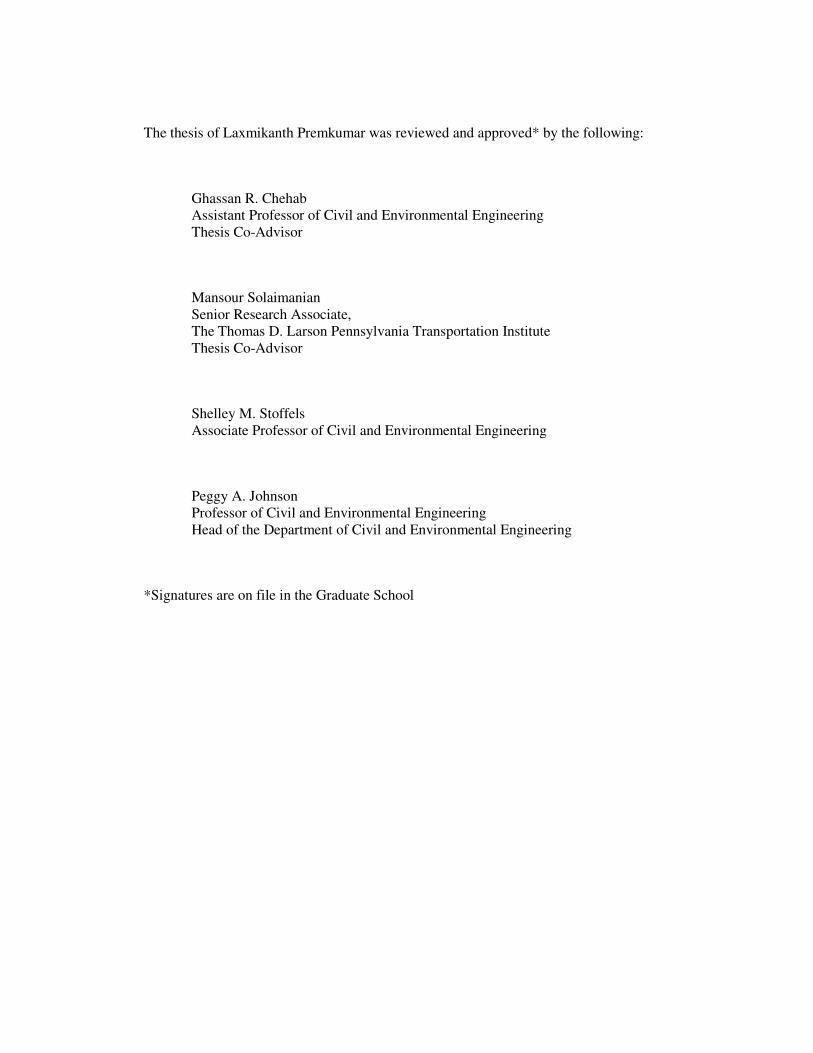
factors of the desired reference temperature to zero and making appropriate changes to shift
factors at other temperatures. Figure 4.9 illustrates this process of shifting the reference
temperature from -22°C to -12°C. It is also possible to develop a master curve by shifting to a
reference temperature outside the range of testing temperatures.
-3
-2.5
-2
-1.5
-1
-0.5
0
0.5
1
1.5
2
-24 -21 -18 -15 -12 -9 -6 -3
Temperature (C)
Lo
g s
hif
t fa
cto
r
Reference -22°C
Reference -12°C
Figure 4.9 Method for shifting the reference temperature

36
The D(t) and S(t) master curves are fitted by means of the sigmoidal and hyperbolic fits as shown
in Equations 4.17 and 4.18 respectively.
( )[ ]
( )[ ]
++
+=
Rtaa
aa
aatD
logexp
log
65
43
21
4.17
where,
D(t) is the creep compliance (1/MPa),
a1 through a6 are regression coefficients, and
tR is the reduced time(s).
( ) ( ) { } 3
22
23 45.0log βλββ +
+−×−= nnt ttS
4.18
where,
( )( )23
log
ββ −
+−= To
n
attt ,
( ) ( )[ ]xx −+=
expexp
2λ ,
X = 0.339*tn + 0.00637* tn 3 ,
t = loading time(s),
S(t) = Flexural creep stiffness (MPa),
aT = temperature shift factor [log(sec)], and
β1, β2 and β3 are regression coefficients.

37
5. TEST METHODS, EQUIPMENT AND PROTOCOL
5.1 TEST EQUIPMENT AND INSTRUMENTATION
The IDT tests are conducted using a closed loop hydraulic universal testing machine
manufactured by Material Test Systems (MTS) and BBR tests are conducted on the bending
beam rheometer machine manufactured by Cannon Instruments.
The MTS system consists of a 100kN (22kip) load cell and actuator which is interfaced with an
MTS® 458.20 MicroConsole. The loading waveform is programmed using an MTS® 458.91
Microprofiler which is part of the Microconsole. Different types of waveforms including
haversine, sine, square, triangle and trapezoidal can be programmed using the Microprofiler. The
waveforms can be programmed as blocks or segments and a program can consist of several
blocks or segments depending on the waveform required.
An MTS® 409.80 temperature controller along with a MIC 2000 Partlow controller is interfaced
with an environmental chamber fitted with an electric heater. Low temperature is obtained by
using liquid nitrogen gas for cooling the environmental chamber. A dummy specimen embedded
with a K-type thermocouple and with properties similar to the actual test specimen is used to
monitor the specimen temperature. The test is conducted only after the specimen stabilizes at the
required test temperature. Data acquisition is performed using a separate computer fitted with a
National Instruments® 6329 DAQ card and data acquisition programs in Labview are used for
data collection. The complete setup is shown in Figure 5.1.
The deformation values are measured by means of Linear Variable Differential Transformers
(LVDTs). For the IDT test, four XS-B LVDTs, with a range of ± 0.25mm are used for measuring
the vertical and horizontal deformations. The deformation values are measured along a gage
length of 25.4 mm for a specimen diameter of 100mm and 38.1mm height.
It is to be noted that a 6” jig, as shown in Figure 5.2, was used for all the IDT tests instead of a 4”
jig. As the deformations are measured close to the centre, the incorrect jig might not have an
effect on the creep compliance values (SHRP -357). However, there could be errors associated

38
with the strength values. In this thesis, corrections for change in jig are not applied considering
that the material properties are utilized for ranking purposes alone.
Figure 5.1 Complete setup of the MTS and Partlow controller
Figure 5.2 IDT test setup
Liquid Nitrogen MicroProfiler
MTS Loading Frame
and Environmental chamber
Partlow Controller
Dummy
Specimen

39
The Bending Beam Rheometer (BBR) is an instrument used to measure the flexural creep
stiffness of asphalt binder over a temperature range of -5˚C to -40˚C in a three point bending
arrangement. The BBR test apparatus consists of three major components: the control unit, the
load unit and the refrigeration unit. The load and the control units are supplied by Cannon
Instruments Inc. while the refrigeration unit is manufactured by JULABO USA Inc. The Julabo
refrigerated circulators employ a circular head and a cooling machine with capabilities of heating
and cooling liquids in bath tanks.
The control unit is the base of the BBR. It contains the electronic components required to
condition the signals from the LVDT, load cell and temperature probe and to communicate with
the host computer via the serial port. Also included in this unit are gages and switches required
for operation and adjustment of the pneumatic system. The load unit consists of a vertical shaft,
the movement of which is measured precisely by an LVDT with a range of 10mm. An air
chamber below the air bearing provides a force that counterbalances the load applied to the
specimen from the entire weight of the load cell. The load applied to the specimen can be
controlled by adjusting the switches on the control unit.
Specifications for the BBR bath liquid require it to have low viscosity, high heat capacity and low
vapor pressure over a wide range of temperatures (AASHTO T313). Ethyl alcohol (200 proof)
which matches the specifications closely was used for this study. The data collection software for
the BBR, BBR version 1.23, developed by Cannon Instruments Inc. was not capable of capturing
data after 240 seconds; therefore, a special software BBR version 3.21 (also known as BBR-
Long) developed by the same company was utilized. This new software is capable of capturing
data for a maximum period of two weeks. For this study, data was collected every 2 seconds for
the 2 hour tests to avoid large data files. The complete setup of BBR is shown in Figures 5.3 and
5.4.

40
Figure 5.3 Complete setup of the BBR
Figure 5.4 BBR test specimen between supports
Temperature
Controller
BBR
Nitrogen
Air

41
5.2 TEST METHODS AND PROTOCOL
5.2.1 MATERIALS AND SPECIMEN FABRICATION
All specimens for IDT testing were obtained from SISSI field mixtures. The details of the
mixtures for all eight sites of the SISSI project were discussed in detail in Chapter 3. As thermal
cracking is more prominent in the wearing layer (OECD, 2005), IDT specimens were only
prepared from the wearing layer of each site.
The materials, available in 50 pound buckets, are heated at 130° C to obtain loose mixtures for
compaction. Then, the loose mixture is conditioned in the oven at 5°C to 10°C above the
respective compaction temperature. This procedure is followed to minimize the heat lost during
the compaction process. Temperature probes are positioned in the mixture to monitor the actual
temperature of the mixture. The compaction temperature and maximum theoretical specific
gravity (Gmm) for the mixtures used are shown in Table 5.1. All specimens are compacted to a
height of 115mm, later cored and cut to obtain two 100mm x 38mm(diameter x height) specimens
for IDT testing. The mass of mixture used for compaction varied for each site based on the Gmm
of the mixture. All specimens were compacted to achieve a target air void content of 7 ± 0.5 % in
the 100mm x 38mm specimens.
Table 5.1 Compaction temperature (°C) and Gmm for wearing layers of SISSI sites
Mixture ID Layer County Compaction Temperature (º C) Gmm
M0264 wearing Tioga 153 2.502
M0272 wearing Mercer E. 153 2.468
M0287 wearing Mercer W. 153 2.486
M1255 wearing Warren 153 2.349
M1261 wearing Perry 169 2.498
M2167 wearing Delaware 168 2.457
M2302 wearing Somerset 153 2.500
M3298 wearing Blair 156 2.535
For the BBR tests, pressure aging vessel (PAV) aged binders from the wearing layers of seven
sites excluding Tioga are utilized for preparing specimens. Typically, asphalt binder undergoes
aging, i.e. becomes brittle due to volatilization of light oils and exposure to oxygen (SP-2, 1993).
After the asphalt pavement is constructed, oxidation dominates the aging process and this in-

42
service aging is simulated by the Superpave™ PAV test. The detailed procedure for preparing
BBR specimens is discussed in AASHTO T313. The steps involved in preparing the specimen are
shown in Figure 5.5.
a
b
c
d
Figure 5.5 Steps involved in preparing a BBR specimen: (a) mold preparation, (b) pouring
the asphalt binder, (c) trimming the surface, (d) sample specimen

43
5.2.1.1 DETERMINING THE IDT SPECIMEN DIMENSIONS AND AIR VOID
CONTENT
Specimens compacted using the gyratory compactor tends to have non-uniform air void
distribution along the diameter and height. From previous studies conducted by Chehab et al.
(2000), it was observed that the top and bottom part of the specimen have significantly higher air
voids and for variation along the diameter, the ring has more air voids than the core. Hence to
obtain uniform air void content, the specimen will have to be cored from a larger specimen with
top and bottom portions cut off. From the study conducted by Chehab et al., it was also observed
that the 100 x 150 mm specimens had the least variation of air voids along their height as shown
in Figures 5.6.
Figure 5.6 Distribution of air void content (%) in gyratory compacted specimens
(Chehab et al., 2000)
Though the 100 x 150 mm (cored from 150 x 175 mm) specimen had the least amount of air
voids, specimen geometry of 115 x 150 mm was selected, keeping in mind the limited material

44
available for specimen fabrication. Though AASHTO 322 specifies specimen geometry of
150mm x 38 mm for IDT testing, all the IDT tests in this study are conducted on 100mm x 38mm
specimens. This specimen geometry is adopted considering the fact that the 150mm diameter
specimens have a greater variation of air void content along its diameter in comparison with the
100mm diameter specimens (Wen, 2000).
Superpave™ mix design procedures require the design air void content to be 4% for laboratory
prepared specimens (Asphalt Institute, 1996), while compaction in the field takes place at 2% to
4% above the design air void content (i.e. 6% to 8%). The objective of the SISSI project involves
predicting pavement performance using the MEPDG, with material characterization test data as
input. In order to get a meaningful comparison between pavement performance predicted from
MEPDG and field observation, it is ideal that material properties, including air void contents, in
the field and laboratory match. Level 1 input for thermal cracking model in the MEPDG requires
tensile strength, creep compliance and air voids content as an input (ARA, 2003). The as
constructed air void content is used to calculate the coefficient of thermal contraction used as
input for the thermal cracking model. Hence, to obtain good correlation between field and
laboratory compacted specimens, as constructed air void content of 7 ± 0.5 % was chosen for
testing purposes. Details on the MEPDG software and the thermal cracking model are available in
a separate report (ARA, 2003).
5.2.1.2 SUPERPAVE™ PG-GRADING SYSTEM
As explained in Chapter 1, a major outcome of the SHRP project was the Superior Performing
Asphalt Pavements (Superpave™) mix design and Performance Grade (PG) binder systems. The
Superpave™ system incorporates performance based testing on asphalt binders and mixtures to
control rutting, low temperature cracking and fatigue cracking in asphalt pavements, i.e. the
properties measured from tests can be related to the field through basic engineering principles
(Asphalt Institute, 1996).
The Superpave™ performance grade asphalt binders are designated by the term PG 64-22, for
example, wherein this binder is designed to sustain the conditions of an environment with an
average seven-day maximum temperature of 64°C and minimum pavement design temperature of
-22°C. The Superpave™ binder specification was designed to limit the susceptibility of the
asphalt binder towards permanent deformation, low temperature and fatigue cracking of

45
pavements. For grading the asphalt binders and to check its susceptibility to various distresses,
several tests as shown in Table 5.2 are conducted at temperatures encountered by in-service
pavements. The Superpave™ binder specification is unique as the testing temperatures are varied,
while the material property values to be achieved remain the same. This is because, for example,
though good performance of asphalts binders is required in both Texas and Pennsylvania;
different types of binders will be required due to varied climatic conditions. Table 5.2 lists the
binder test equipments along with a brief description of why the test is used for Superpave™
specifications. Figure 5.7 describes how the tests are indicative of the binder performance.
However, the mixture properties and the pavement structure will also play a part in the
performance of the overall structure.
Table 5.2 Superpave™ binder test equipment (Asphalt Institute, 1996)
EQUIPMENT PURPOSE
Rolling Thin Film Oven (RTFO)
Simulate binder aging (hardening) characteristics
Pressure Aging Vessel (PAV)
Dynamic Shear Rheometer (DSR) Measure binder rheological properties
at high and intermediate service temperatures
Rotational Viscometer (RV) Measure binder viscosity at high temperatures
Bending Beam Rheometer (BBR) Measure low temperature stiffness and failure
properties.
Direct Tension Tester (DTT)

46
Handling
pumping
Thermal
cracking
Fatigue
cracking
Permanent
deformation
flow
rutting
structural
cracking
thermal
cracking
Rotational Viscometer
Dynamic Shear
Rheometer
Bending Beam Rheometer
Direct Tension Tester
Test Equipment Performance Property
Figure 5.7 Relation of the Superpave™ binder tests to performance (Asphalt Institute, 1996)
5.2.2 IDT TESTING PROGRAM FOR ASPHALT MIXTURES
The IDT tests for D(t) and tensile strength are conducted in accordance with AASHTO 322. X-
SB LVDTs, two each for measuring the vertical and horizontal deformations are fitted onto the
specimen by means of LVDT mounts. Eight brass gage points having a diameter of 8mm and
height of 3.2mm, glued using a Devcon 5-minute epoxy are used to fit the mounts onto the
specimen. A special template is used to facilitate this process. After securing the screws on the
mounts, the LVDT signals are checked to ensure that each LVDT is measuring near the middle of
its range and is repositioned if required.
A gage length of one inch (25.4 mm) is used for mounting the LVDTs as specified by AASHTO
322. Use of larger LVDT gage lengths minimizes the effects due to large aggregate particles
between the gage points. But considering the fact that the viscoelastic solutions developed by
Wen (2001), used in this study to calculate the D(t) of the mixtures, did not accommodate for
38.1 mm gage length and to minimize the effects due to stress concentrations near the loading
strips, a gage length of 25.4mm is deemed appropriate since the nominal maximum aggregate size

47
for the wearing layers of all SISSI sites is 12.5 or 9.5mm. The horizontal and vertical LVDT
setup is shown in Figure 5.8.
D(t) tests are conducted for a 100 second loading time at -20,-10 and 0oC by loading the
specimens along the diametric axis to produce vertical and horizontal deformations. Specimens
are tested at the lowest temperature first and progressively at higher temperatures. At low
temperatures, the X-SB LVDT coils tends to freeze and stall during testing. In such cases, the
environmental chamber is left open to defreeze the LVDT’s before testing at the test temperature.
Prior to testing, to check the positioning of the specimen, a small creep load for a period of 20
seconds is applied. The position of the specimen on the jig is later adjusted, if required, to attain
similar deformations on the horizontal and vertical LVDTs on both sides. The AASHTO
specifications stipulate that the asphalt concrete specimen remain in linear viscoelastic range (i.e.
no damage) throughout the creep test. This can be achieved by maintaining the horizontal strains
within 0.05% (AASHTO T322). In this study, loads are applied to maintain the horizontal strains
within 0.01% (Wen, 2001), considering the fact that the specifications are for 150mm diameter
specimens. If this limit is reached, the test is stopped immediately and the specimens are allowed
to relax for a minimum of 5 minutes before resuming with appropriate load levels.
Figure 5.8 LVDT setup on the IDT specimen
Once all D(t) testing is completed, the specimens are cooled to -10oC to conduct the tensile
strength test by loading the specimens at a constant crosshead movement rate of 12.5 mm/sec
until failure. In this study, the LVDT’s are removed prior to strength tests, to avoid any damage

48
caused due to possible catastrophic specimen failure (NCHRP 530). The tensile strength of the
mixtures is calculated using Equation 2.4.
5.2.3 BBR TESTING PROGRAM
The BBR is used to obtain the flexural creep stiffness S(t) of PAV-aged SISSI binders, by loading
beam specimens in a three point bending arrangement. The test specimens are 5-inch by 0.5 inch
by 0.25 inch beams simply supported at a span length of 4 inches. The asphalt beam is loaded at
mid span with load applied using a pneumatic actuator and piston guided by air bearing. Creep
load is then applied and held constant for the required test duration. The loads are varied
according to the temperature and asphalt stiffness to maintain the strain response within the linear
viscoelastic range, i.e. within 0.5% (Bahia, 1991).
Superpave™ specifications require the testing to be conducted for a period of 240 seconds at a
test temperature of 10°C higher than the lower temperature grade of the asphalt binder (AASHTO
T313). This specification was developed with the assumption that the flexural creep stiffness of
the asphalt binder at 2 hours [S(7200)] at the temperature of the lower temperature grade is
equivalent to its flexural creep stiffness at 60s [S(60)] at a temperature 10°C higher. This was
concluded through comprehensive studies conducted by Anderson et al. (1992) proving that the
shift factor curve for all asphalt binders are similar and have, approximately, a slope between
0.173 log(s)/° C and 0.199 log(s)/°C. Details of the study can be found in the SHRP reports
(Anderson et al., 1994). As the main aim of this study is to revisit and build on the research
conducted previously, it is required to obtain the S(t) of the asphalt binders at the lowest binder
grade temperature, at a temperature 10°C higher than the lower temperature grade of the binder
and a temperature of -5°C for the purpose of constructing a stiffness master curve. Initially, a
temperature of 0°C was used for testing, but due to problems with applying low loads to maintain
linear viscoelastic response, a temperature of -5°C was chosen (Bahia, 1991). As the low
temperature grade for all the asphalt binders tested in this study is the same (XX-22), henceforth
the lower temperature grade will be referred to as T1.
In order to satisfy both objectives of this study, to verify if S(7200) at T1 is equal to S(60) at T1
+10 and to check if all asphalt binders have similar shift factor curves, BBR tests had to be
conducted for both 240 seconds and 2 hours at all three temperatures. Master curves are
developed individually for the 2 hour and 240 second data for comparison and verification. At

49
each temperature, the 240 second test is conducted prior to the 2 hour test and the stiffness values
are compared to make sure the specimen is in the linear viscoelastic range. Marasteanu and
Anderson (2000) specified that in order for the asphalt binder to be LVE, the conditions for
homogeneity and superposition must be satisfied. The check for homogeneity is considered
satisfied if the asphalt binder stiffness remains within 5% after testing at various loads at a given
temperature. In this study, the condition for LVE is checked by conducting 240 second tests
immediately after the 2 hour test with same or increased load levels. It is observed that the
stiffness values at 60 seconds for the final 240 second tests were higher than those of the 2 hour
tests at all three testing temperatures, proving the specimen is in LVE range as shown in Figure
5.9.
The specimens were marked to make sure they remain in the exact same position for all
temperatures during the test. During initial testing, the displacement values at the beginning and
end of each test, at every temperature, were recorded to check if the specimen relaxed to its
original position. Alternative methods to check the specimen relaxation, like recording the
relaxation data (Marasteanu and Anderson, 2000) could prove to be more effective. Due to time
constrains, it was decided that a relaxation time of 20 minutes and 2 hours after the 240 second
and 2 hour tests respectively, should be sufficient. The relaxation times were chosen keeping in
mind the total time of testing and it could be possible that the specimen did not relax to its
original position with the relaxation times provided. The relaxation times were primarily provided
to ensure that the specimen remains in LVE range throughout the course of the test. However, for
all BBR tests, LVE condition was satisfied by means of the homogeneity principle which
overrides any insufficient relaxation time.

50
0
100
200
300
400
500
600
700
0.1 1 10 100 1000
Time(s)
S(t
) 1
/Mp
a
240s test-initial
2hr test
240s test- after2hr test
Mercer west - replicate 2
Test temperature -5°C
Figure 5.9 Check for LVE conditions
Initially a dummy specimen was placed inside the control unit water bath to monitor the exact
temperature of the test specimen. But it was observed that the dummy specimen required less than
10 minutes to reach the testing temperature. AASHTO specifications require the specimen to be
conditioned at the test temperature for one hour before testing. In this study, due to the
introduction of a 2hr relaxation time between temperatures, the conditioning time is considered
more than sufficient. Hence, the dummy specimen was not utilized to monitor temperatures for
subsequent tests. It is to be noted that after the completion of a 2 hour test at a particular
temperature, the temperature of the bath is changed to the subsequent test temperature. Ideally,
the specimen must be allowed to relax for 2 hours at the current test temperature to avoid any
possible effects associated with the coefficient of thermal expansion of the asphalt binder
specimen. But, due to time constraints, the time taken for change in temperature is also included
in the relaxation time.
Before each test, the standard calibration procedures are followed, which are explained in detail
in AASHTO T313. While placing the test specimen between the supports, it is observed that the
specimen slid away from the supports due to the forces exerted by ethanol circulating in the liquid
bath. To circumvent this problem, the vertical shaft has to be brought down to apply a small load
and hold the specimen in position. Later, a valve was fitted to control the flow of ethanol

51
circulating in the bath which eliminated this problem. Between testing temperatures, the test
specimen is removed from its supports and placed inside the bath to eliminate any creep from self
load.
During initial periods of testing, creeping of the load with time was observed both during the 240
second and 2 hour tests, as shown in Figure 5.10. The load increased by up to 50% during certain
tests, especially at higher temperatures. Similar problems were also noticed during the SHRP
projects (Bahia, 1991), but no concrete solution was available to solve this problem. The front
panel of the BBR was replaced and a needle valve installed (to assist the ramp in a square wave)
to reduce the increase in load during the creep tests. Finally it is observed that by placing the
thick steel specimen (utilized for calibration) in load mode for an hour before testing solves the
problem.
0
50
100
150
200
250
300
350
0 1000 2000 3000 4000 5000 6000 7000
time(s)
Fo
rce
(mN
)
After
Before
Figure 5.10 Loading curve before and after installation of needle valve

52
Time(s)
240s
loading
2hr
loading240s
loading
1200s
recovery7200s
recovery
Load
Deflection
Next test temperature
300s
recovery
Figure 5.11 BBR testing protocol for one test temperature

53
6. RESULTS AND ANALYSIS
6.1 D(t) AND TENSILE STRENGTH OF SISSI MIXTURES
The IDT tests are conducted on specimens from all eight SISSI sites as described in Chapter 5.
The number of replicates tested for each site along with the air void content is shown in Table
6.1. Though the target air void is 7 ± 0.5 %, some of the replicate specimens from the SISSI sites
are off target due to material quantity constraints.
Table 6.1 Air void content (%) and number of replicates for SISSI - IDT specimens
SISSI Site Replicate number Air void content(%)
Blair 1 6.5
2 6.9
Delaware 1 6.3*
2 6.8
Mercer East 1 7.2
2 7.6*
Mercer West 1 6.3*
2 6.6
Perry 1 6.5
2 6.7
Somerset 1 6.6
2 6.8
Tioga 1 8.9*
2 9*
Warren 1 6.6
2 6.7
3 7.2
4 7.5
* specimens with AV% off target

54
Figure 6.1.1 represents the D(t) vs. time chart for both replicates of the Mercer East site. The D(t)
vs. reduced time and extended sigmoidal fit at reference temperature of -10°C are shown in
Figures 6.2 and 6.3 respectively. The shift factor curve and sigmoidal coefficients for both the
replicates are shown in Figure 6.4 and Table 6.2 respectively. IDT test data for the other SISSI
sites are documented in Appendix A.
0.00E+00
6.00E-05
1.20E-04
1.80E-04
2.40E-04
1.00E-03 1.00E-01 1.00E+01 1.00E+03
Time(s)
D(t
) 1
/Mp
a
0C -7.2%
-10C -7.2%
-20C - 7.2%
0C - 7.6%
-10C -7.6%
-20C -7.6%
Figure 6.1 Creep compliance vs. time for replicates of Mercer East in semi-log domain

55
0.00E+00
6.00E-05
1.20E-04
1.80E-04
2.40E-04
1.00E-03 1.00E-01 1.00E+01 1.00E+03 1.00E+05
Reduced time(s)
D(t
) 1
/Mp
a
Reference -10°C
7.2%
7.6%
Figure 6.2 Creep compliance vs. reduced time for replicates of Mercer East in semi-log domain
3.00E-05
7.00E-05
1.10E-04
1.50E-04
1.00E-04 1.00E-02 1.00E+00 1.00E+02
Reduced time (s)
D(t
) 1/M
pa
7.60%
7.20%
Average
Reference -10°C
Figure 6.3 Extended sigmoidal fit for replicates of Mercer East in semi-log domain

56
y = -0.004x2 - 0.2072x - 1.6701
R2 = 1
y = -0.0046x2 - 0.2225x - 1.7607
R2 = 1
-2
-1.5
-1
-0.5
0
0.5
1
-21 -16 -11 -6 -1 4
Temperature (C)
Lo
g s
hif
t fa
cto
r
AV % = 7.6
AV % = 7.6
Figure 6.4 Shift factor curve for replicates of Mercer East
Table 6.2 Sigmoidal coefficients for Mercer East
7.20 (% AV) 7.60 (% AV)
A1 7.88576693 7.917016431
A2 -29.07045919 -29.06715893
A3 2.36672053 2.363894395
A4 2.87353936 2.932640128
A5 4.635804919 4.446491814
A6 -0.402479796 -0.369121547
The difference in creep compliance between replicates for all SISSI sites was observed to be
within 30% which follows the values reported in NCHRP 530. It is to be noted that the
differences stated are only for the testing times and not for data extrapolated using the sigmoidal
function. The average creep compliance data shifted to a reference temperature of -10°C and
tensile strength data for all the SISSI sites are shown in Figures 6.5 and 6.6, respectively. The
ranking of specimens based on the creep compliance and tensile strength of the mixtures is
discussed in section 6.4.

57
2.00E-05
1.20E-04
2.20E-04
1.00E-03 1.00E-01 1.00E+01 1.00E+03
Reduced time (s)
D(t
) 1
/Mp
a
Somerset
Tioga
Mercer East
Mercer West
Perry
Blair
Warren
Delaware
Figure 6.5 Creep compliance master curves for all SISSI sites at reference temperature of -10°C
0.00
1.00
2.00
3.00
4.00
5.00
Blair Delaware Mercer east Mercer west Perry Somerset Tioga Warren
SISSI site
Ten
sile
str
eng
th (
Mp
a)
Figure 6.6 Average tensile strength values for all SISSI sites

58
6.2 FLEXURAL CREEP STIFFNESS AND M-VALUES OF SISSI BINDERS
BBR tests are conducted on PAV aged asphalt binders for seven of the eight SISSI sites. Tests
were not conducted for Tioga due to lack of material. Two replicates from each site are tested for
S(t) at 240 second and 2 hour durations. The detailed test procedure has been presented in
Chapter 5. Figures 6.7 through 6.9 and Table 6.3 represent the S(t) vs. time, creep stiffness master
curves, shift factor curves and hyperbolic coefficients for the 240s BBR test for both replicates
from Somerset. Data for the other SISSI sites are shown in Appendix B.
0
200
400
600
800
1000
1200
1 10 100 1000
Time(s)
S(t
) M
pa
-22C Somerset 1
-12CSomerset 1
-5C Somerset 1
-22C Somerset 2
-12C Somerset 2
-5C Somerset 2
Figure 6.7 Flexural creep stiffness vs. time for Somerset on a semi-log scale

59
10
260
510
760
1010
0.1 1 10 100 1000 10000
Reduced time (s)
S(t
) M
pa
Somerset -replicate 2
reference -11.88°C
Somerset -replicate 1
reference -11.87°C
Figure 6.8 Flexural creep stiffness vs. reduced time for Somerset on a semi-log scale
y = -0.1285x - 1.4434
R2 = 0.9958
y = -0.1337x - 1.5604
R2 = 0.9996
-1
-0.5
0
0.5
1
1.5
2
-25 -20 -15 -10 -5 0
Temperature (C)
Lo
g s
hif
t fa
cto
r
Somerset -replicate 2
Somerset -replicate 1
Figure 6.9 Shift factor curves for Somerset on a semi-log scale

60
Table 6.3 Hyperbolic fit coefficients
Somerset 1 Somerset 2
β2 1.61 1.59
β3 3.22 3.27
To 3.55 3.65
The comparison of average D(t) and m-values at 60 seconds at T1+10 for two replicates from the
SISSI sites is shown in Figure 6.10 and 6.11, respectively. The ranking of the SISSI sites with
respect to S(t) and m-value is discussed in section 6.5 of this chapter. Both the S(t) and m-value
criteria are not satisfied for both Perry and Delaware. Modified asphalt binders are normally more
flexible than unmodified binders to satisfy the specification criteria over a broader temperature
range and typically tend to have lower stiffness values (SHRP-A-631). However, from this study,
the modified asphalt binders with the exception of Perry have higher S(t) values compared to the
unmodified asphalt binder.
253
297
251 259
330
220
355
0
50
100
150
200
250
300
350
400
Warren Blair Somerset Mercer
East
Mercer
West
Perry Delaware
SISSI site
S(t
) M
pa
Figure 6.10 Comparison of average S(60) at T1+10 for SISSI sites

61
0.32250.3345 0.338
0.2910.332
0.296
0.372
0
0.05
0.1
0.15
0.2
0.25
0.3
0.35
0.4
Warren Blair Somerset Mercer
East
Mercer
West
Perry Delaware
SISSI site
m-v
alu
e
Figure 6.11 Comparison of m(60) at T1+10 for SISSI sites
The change in m-value with increase in temperature and duration of the test is shown in Figure
6.12. It is observed that the m-value generally increases with temperature, as expected due to the
increase in viscoelastic behavior of asphalt binders. Detailed results for all the sites are shown in
Table C1 in Appendix C. The m-value for all the sites follows a similar pattern. However, no
definite correlation is observed between the m-values obtained from the 240 second and 2 hour
tests.

62
0.241
0.341
0.433
0.231
0.33
0.432
0
0.05
0.1
0.15
0.2
0.25
0.3
0.35
0.4
0.45
0.5
-22 -12 -5Temperature (C)
M-v
alu
eSomerset-240s
Somerset -2hr
Figure 6.12 Comparison of m(60) at T1+10 for 240s and 2hr BBR tests for Somerset
Table 6.4 presents the S(t) values obtained from the BBR software and predicted from the
hyperbolic equation. For example, the S(60) obtained directly from the 240 second BBR test at
actual testing temperature are shown in Column One. The S(60) at T1+10 predicted using the
hyperbolic equation (Equation 4.4.5) for the 240s test is shown in Column Two. Similarly,
Column Four (4) and Column Five (5) and Column Seven (7) and Column Eight (8) represent the
actual and predicted S(60) and S(7200) at T1 respectively. From columns 5 and 8 of Table 6.4, it
is observed that for all the SISSI asphalt binders tested, the equivalence principle is not satisfied.
From Figure 6.13, the percent difference between S(60) at T1+10 and S(7200) at T1, based on the
stiffness at 60s @ T1 [i.e. from Table 6.4], calculated as( )
( )
−100*
5
85
column
columncolumn] ranges
from 41% to 52% and appears to be consistent. It is to be noted that the equivalence principle for
all the SISSI asphalt binders is evaluated based only on data obtained from the 2 hour testing.
Hence, to satisfy the equivalence principle, it is necessary to adopt alternate testing times or
temperatures for the SISSI asphalt binders as shown in Figures 6.14 and 6.15 respectively. Figure
6.14 represents the predicted time to test for the SISSI binders at T1+10 to satisfy the equivalence
principle and ranges from 240 seconds to 450 seconds. However, the current BBR software used,

63
(BBR 1.23) is only capable of collecting data up to 240 seconds. To avoid complications in
collecting test data, alternate testing temperatures are also predicted as shown in Figure 6.15. The
alternate testing temperatures predicted ranges from -5°C to -8°C indicating that the SISSI
binders must be tested on an average, at 15°C higher than the lower temperature grade to satisfy
the equivalence principle. The percent difference, actual time and temperature values predicted
for the SISSI binders are shown in Table 6.5.

64
Table 6.4 Actual and predicted flexural creep stiffness values (MPa) for SISSI binders
Column number 1 2 3 4 5 6 7 8
Test duration:240s Test Duration:2-hr
S(t) @ 60s @ S(t) @ 60s @ S(t) @ 7200s @
SISSI Site
Test Temp -12C Test Temp -12C Test Temp -22C
Warren–replicate 1 241.5 (-12.05) 249.60 242.1(-12.08) 249.70 152(-22.29) 147.00
Warren–replicate 2 238.2(-11.99) 256.90 248.2(-11.98) 264.50 149.1(-22.17) 144.60
Blair-replicate 1 274.2(-11.88) 279.90 282.8(-11.89) 297.10 177.5(-23.05) 155.70
Blair-replicate 2 315.9(-11.92) 314.41 320.6(-11.91) 338.20 195.6 (-22.2) 189.20
Somerset-replicate 1 230.3(-11.88) 238.10 235.2(-11.85) 242.10 140.8(-22.17) 137.10
Somerset-replicate 2 246.3(-11.88) 264.00 256.2(-11.86) 272.60 149(-22.08) 146.80
Mercer East-replicate 1 234.4(-11.71) 261.30 239.8(-11.71) 253.00 144.1(-21.96) 144.80
Mercer East-replicate 2 228.5(-11.6) 257.00 232.2(-11.6) 258.30 143.1(-21.9) 143.50
Mercer West-replicate 1 297.7(-11.94) 332.00 312.8(-11.93) 329.50 185.2(-22.06) 182.10
Mercer West-replicate 2 300(-11.88) 327.60 313.2(-11.88) 333.50 181.2(-22.05) 178.20
Perry-replicate 1 208.4(-11.99) 221.9 213(-11.99) 222.8 123.7(-22.43) 120.3
Perry-replicate 2 214.5(-11.96) 217.5 219.3(-11.95) 227 118.5(-22.43) 110.7
Delaware-replicate 1 356.5(-12.09) 352 354(-12.07) 364.5 219.2(-22.49) 210.2
Delaware-replicate 2 352.5(-12.06) 357.4 370.8(-12.05) 375.4 219.5(-22.49) 206.5
* values in brackets represent the actual test temperature

65
0
10
20
30
40
50
Warren Blair Somerset Mercer
East
Mercer
West
Perry Delaware
SISSI Site
Ave
rag
e %
dif
fere
nc
e b
etw
ee
n S
(60
) a
t T
1+
10
an
d S
(720
0)
at
T1
Figure 6.13 Average % differences between S(60) @ T1 +10 and S(7200) @ T2
0
50
100
150
200
250
300
350
400
450
500
Warren Blair Somerset Mercer
East
Mercer
West
Perry Delaware
SISSI Site
Ave
rag
e p
red
icte
d t
ime(s
)
Figure 6.14 Average predicted time for S(60) @ T1 +10 and S(7200) @ T2 to be equivalent

66
-9.0
-8.0
-7.0
-6.0
-5.0
-4.0
-3.0
-2.0
-1.0
0.0
Warren Blair Somerset
Mercer
East
Mercer
West Perry Delaware
SISSI Site
Ave
rag
e p
red
icte
d t
em
pe
ratu
re (
C)
Figure 6.15 Predicted temperatures for S(60) @ T1 +10 and S(7200) @ T2 to be equivalent

67
Table 6.5 % Difference, actual time and temperature predicted for SISSI sites
Column number 1 2 3
SISSI Site Difference Actual Time Temp for
60s
(%) (s) (°C)
Warren-replicate 1 41 443 -7.5
Warren-replicate 2 45 317 -6.7
Blair-replicate 1 48 395 -6.0
Blair-replicate 2 44 326 -6.5
Somerset-replicate 1 43 284 -7.1
Somerset-replicate 2 46 323 -6.6
Mercer East-replicate 1 43 247 -7.8
Mercer East-replicate 2 44 266 -7.5
Mercer West-replicate 1 45 381 -5.7
Mercer West-replicate 2 47 407 -5.3
Perry-replicate 1 46 340 -6.2
Perry-replicate 2 51 411 -5.3
Delaware-replicate 1 42 340 -5.9
Delaware-replicate 2 45 360 -5.7
Average 45 346 -6.4
Figure 6.16 shows the comparison of average shift factors for the SISSI and SHRP asphalt
binders (Bahia, 1991). As discussed in Chapter 2 (Table 2.2 and Figure 2.8), the shift factor
functions for all asphalt binders are considered to be similar and the slope of the shift factor curve
is found to have a common slope between 0.173 log(s)/° C and 0.199 log(s)/°C. From Figure 6.16
and Table 6.6, it is observed that all the SISSI binders have similar shift factors. However, the
slope of the shift factor curve varies between 0.111 log(s)/° C and 0.142 log(s)/°C and thus
contradicts the fact that all asphalt binders have similar shift factors. The SHRP asphalt binders’
shift factors are calculated at a reference temperature of -15°C. For comparison, all the SISSI
asphalt binders’ and the SHRP asphalt binders’ shift factors are shifted to a reference temperature
of -12°C (i.e. the log shift factor values is zero at -12°C).

68
Table 6.6 Slope and R2 for shift factor curves for binders from the SISSI sites
SISSI Slope (%) R2
Warren 1 -0.1395 0.9986
Warren 2 -0.1269 0.9919
Blair 1 -0.1244 0.9994
Blair 2 -0.131 0.9994
Somerset 1 -0.1337 0.9996
Somerset 2 -0.1285 0.9958
Mercer East 1 -0.1344 0.9962
Mercer East 2 -0.1346 0.9961
Mercer West 1 -0.1418 0.9863
Mercer West 2 -0.1183 0.9914
Perry 1 -0.1227 0.9939
Perry 2 -0.1204 0.9998
Delaware 1 -0.1114 0.9999
Delaware 2 -0.1338 0.9996
Average SISSI -0.1287 0.9963
Average SHRP -0.1831 0.9991
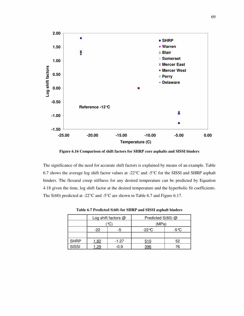
69
-1.50
-1.00
-0.50
0.00
0.50
1.00
1.50
2.00
-25.00 -20.00 -15.00 -10.00 -5.00 0.00
Temperature (C)
Lo
g s
hif
t fa
cto
rs
SHRP
Warren
Blair
Somerset
Mercer East
Mercer West
Perry
Delaware
Reference -12°C
Figure 6.16 Comparison of shift factors for SHRP core asphalts and SISSI binders
The significance of the need for accurate shift factors is explained by means of an example. Table
6.7 shows the average log shift factor values at -22°C and -5°C for the SISSI and SHRP asphalt
binders. The flexural creep stiffness for any desired temperature can be predicted by Equation
4.18 given the time, log shift factor at the desired temperature and the hyperbolic fit coefficients.
The S(60) predicted at -22°C and -5°C are shown in Table 6.7 and Figure 6.17.
Table 6.7 Predicted S(60) for SHRP and SISSI asphalt binders
Log shift factors @ Predicted S(60) @
(°C) (MPa)
-22 -5 -22°C -5°C
SHRP 1.82 -1.27 510 52
SISSI 1.29 -0.9 396 76

70
0
100
200
300
400
500
600
-22°C -5°CTemperature (C)
Pre
dic
ted
S(6
0)
Mp
a
SHRP
SISSI
Figure 6.17 Predicted S(60) at -22°C and -5°C for SHRP and SISSI asphalt binders
From Figure 6.17, it is observed that the S(60) at -22°C and -5°C are different for the SISSI and
SHRP asphalt binders. The observed difference between S(60) at -22°C and -5°C, respectively,
for the SHRP and SISSI asphalt binders is 22% and 46%. The coefficients used to predict the
flexural stiffness values are shown in Table 6.8. The coefficients are usually determined by
regression analysis when performing time-temperature superposition. In this case, the coefficients
are average values of all SISSI asphalts binders. It is understood that using different coefficients
could possibly show varied results in terms of % difference of the flexural stiffness values. But, in
a broader perspective, the need for accurate shift factor values is critical.
Table 6.8 Hyperbolic fit coefficients
Β2 1.5
Β3 3
To 3.5

71
6.3 COMPARISON OF D(t) AND S(t) SHIFT FACTOR FUNCTIONS
The average shift factor values from the IDT and BBR tests at a reference temperature of -12°C
are shown in Figure 6.18. It is observed that the shift factor functions for the S(t) and D(t) test
data are comparable at higher temperatures with exception to Delaware. There exists considerable
variation in shift factor values at -22°C as seen from Figure 6.18. At very low temperatures,
asphalt concrete or asphalt binders tend to be elastic and the S(t) and D(t) curves are nearly
parallel to the time axis. Thus, while shifting S(t) and/or D(t) data to develop the master curves;
several shift factor values for very low temperatures can be used to obtain a smooth and
continuous master curve as shown in Figures 6.18, 6.19 and 6.20. This could be one possible
reason causing the variation of shift factor values at low temperatures for the IDT and BBR tests
of SISSI mixtures and binders.
-2.00
-1.50
-1.00
-0.50
0.00
0.50
1.00
1.50
2.00
-2.00 -1.50 -1.00 -0.50 0.00 0.50 1.00 1.50 2.00
Shift factors from BBR test
Sh
ift
fac
tors
fro
m ID
T t
es
t
Mercer West
Mercer East
Blair
Warren
Somerset
Perry
Delaware
Reference -12°C
-5°C
-22°C
Figure 6.18 Average shift factors obtained from IDT and BBR tests

72
0.00001
0.0001
0.001
0.01
0.01 0.1 1 10 100
Time(s)
D(t
) 1
/Mp
a
-20
-10
0
1.00E-05
1.00E-04
1.00E-03
1.00E-04 1.00E-02 1.00E+00 1.00E+02
Reduced time (s)
D(t
) 1/M
pa
-20
-10Log shift factor @ -20°C = 1.9
reference temperature = -10°C
Figure 6.19 (a) Parallel D(t) curves at low temperatures, (b) D(t) master curve with log shift
factor of 1.9 @ -22°C

73
1.00E-05
1.00E-04
1.00E-03
1.00E-04 1.00E-02 1.00E+00 1.00E+02
Reduced time (s)
D(t
) 1
/Mp
a
-20
-10Log shift factor @ -20°C = 1.6
reference temperature = -10°C
Figure 6.20 D(t) master curve with log shift factor of 1.6 @ -22°C

74
1.00E+00
1.00E+02
1.00E+04
1.00E-02 1.00E+00 1.00E+02 1.00E+04
Reduced time (s)
S(t
) M
pa
-20
-10
Reference temperature = -12°C
Log shift factor @ -22°C = 1.5
1.00E+00
1.00E+02
1.00E+04
1.00E-02 1.00E+00 1.00E+02 1.00E+04
Reduced time (s)
S(t
) M
pa
-20
-10
Reference temperature = -12°C
Log shift factor @ -22°C = 1.3
Figure 6.21 (a) D(t) master curve with log shift factor of 1.5 @ -22°C (b) D(t) master curve with
log shift factor of 1.3 @ -22°C

75
From Figure 6.19(a) it is observed that the D(t) curves of the asphalt mixture at low temperatures
tend to be parallel to each other due to their nearly elastic nature. Figure 6.19(b) and 6.20 shows
the D(t) master curve developed at a reference temperature of -10°C using different shift factors
for -20°C. It can be observed that the curves tend to overlap with each other even with differences
in shift factor values. Though the difference in log shift factor is relatively small, it is magnified
when the shift factor is calculated. Similar example for the S(t) master curve of the asphalt binder
is shown in Figure 6.21. The shift factor values for both D(t) and S(t) curves are shown in Table
6.9.
Table 6.9 Shift factor values for D(t) and S(t) master curves for -20°C with
reference temperature of -10°C
Log shift factor Shift factor
1.9 79.4 D(t)
1.6 39.8
1.5 31.6 S(t)
1.3 20.0
While shifting the master curve to a desired reference temperature, the creep compliance [D(t)] of
the mixture and/or the flexural creep stiffness of the binder remains constant causing the reduced
frequency to change. Or in other words, the master curve only shifts along the horizontal time
axis. The reduced time is calculated as the product of time and shift factor. From the table above
it is observed that the there could be up to 50% variation in the shift factor values, thus producing
huge differences in the reduced time. However, these shift factors are still capable of producing
reasonable master curves as observed from Figures 6.19, 6.20 and 6.21. Hence extra care must be
exercised when calculating the shift factor values at very low temperatures.

76
6.4 RELATIONSHIP BETWEEN LOW TEMPERATURE PROPERTIES OF SISSI
MIXTURES AND BINDERS
As thermal cracking is dependent on both the properties of the asphalt mixtures and binders, it is
important to correlate their D(t) and/or S(t) and m-values. Figure 6.22 and 6.23 show the
comparison of D(t) and/or S(t) and m-values, respectively, for the all SISSI sites with the
exception of Tioga. No definite correlation exists between the D(t) and S(t) data. However, Blair,
Mercer West, Somerset, Tioga and Warren tend to follow a linear pattern.
The m-values of the mixture are in the range of 0.2 to 0.49 compared to binder m-values with a
range of 0.29 to 0.27. With the exception of Delaware, Blair and Perry, the mixture m-values are
lower than that of the asphalt binder. This is expected owing to the elastic nature of the
aggregates, with an m-value of zero and a primary component of asphalt concrete mixtures.
However, to better correlate the relationships between asphalt mixtures and binders, a detailed
analysis incorporating other mixture properties such as air void content, gradation and others
must be performed. However, that is beyond the scope of this study.
1.00E-05
1.00E-04
1.00E-03
1.00E+01 1.00E+02 1.00E+03 1.00E+04
S(t) Mpa (binder)
D(t
) 1
/Mp
a (
mix
ture
)
Mercer East
Mercer West
Somerset
Blair
Warren
Perry
Delaware
Reference -10°C
Figure 6.22 Comparison of average creep compliance/stiffness data for SISSI mixtures and binders

77
0.00
0.10
0.20
0.30
0.40
0.50
Warren Blair Somerset Mercer
East
Mercer
West
Perry Delaware
SiSSI Site
m-v
alu
e
BBR
IDT
Figure 6.23 Comparison of average m-value for SISSI mixtures and binders

78
6.5 RANKING OF SISSI SITES BASED ON IDT AND BBR MATERIAL PROPERTIES
All the SISSI sites with exception of Tioga are ranked for susceptibility of thermal cracking based
on the IDT and BBR test results as shown in Table 6.10.The ranking of all SISSI sites based on
mixture data is shown in Table 6.11. The sites are ranked from 1 to 8 based on their susceptibility
to thermal cracking, i.e. 1 is least susceptible and 8 are the most susceptible. The ranking is based
on the following observations and assumptions.
• S (t) (binder stiffness): It is assumed that the lower the binder stiffness, the less
susceptible the mixture is to thermal cracking.
• Binder m-value: m-value of the binder represents the rate of stress relaxation and, hence,
the ability to absorb more stresses developed in the pavement structure. Thus, binders
with higher m-values are assumed to have the least susceptibility to thermal cracking.
• Mixture m-value: The same concept as that of the m-value for asphalt binders is adopted
for ranking the SISSI sites.
• Tensile strength: Generally, if the strength of the mixture is high, it is less susceptible to
thermal cracking. Hence in this study, the sites were ranked based on tensile strength, i.e.
high tensile strength leads to lower susceptibility to thermal cracking. The tensile strength
and thermal stresses obtained from a typical BBR and DSR test is shown in Figure 6.24.
• D(t) [Creep compliance of the mixture]: The higher the creep compliance, the lower the
complex modulus of the mixture. Hence, sites with higher creep compliance are assumed
to have lower susceptibility to thermal cracking.
The S(t) and m-values of asphalt binder are calculated at -12°C and time of 60 seconds. From
Figure 6.5, it is observed that the m-value of the creep compliance curve varies with respect to
time. But the m-value of the asphalt mixture is calculated as the maximum slope of the D(t)
master curve. The D(t) data at 60 seconds at -10°C and the strength data calculated at -10°C are
considered for ranking the SISSI sites. The ranking of the sites with respect to D(t) of the mixture
might vary if times greater than 100 seconds are considered due to overlapping of the curves, but
for the sake of comparison values at D(t) at 60s is taken into account. The creep compliance
master curve at -12°C will shift only along the time axis with the same creep compliance values.
Hence the ranking of the sites at -10°C and -12°C will be the same at 60s. The ranking of the sites
varies with material property and an overall ranking could not be derived.
From Table 6.10, with exception to tensile strength and m-value of the mixture, Delaware is most
prone to thermal cracking of the SISSI sites, which is also evident from the field observations as

79
shown in Figure 6.25. Correlating the laboratory test data with field observations could provide
an insight on the susceptibility to thermal cracking. Another important observation from Table
6.10 is that no single low temperature material property can be utilized for ranking the mixture
for thermal cracking susceptibility, which is evident from the difference in rankings of the SISSI
sites. Thus, developing a system by assigning weights for the low temperature material properties
will be useful to achieve an overall ranking for the SISSI sites.
Temperature
Tensile Strength
Thermal Stress
Cracking Temperature
Str
en
gth
an
d S
tress
Figure 6.24 Tensile strength and thermal stress obtained from BBR and DSR testing

80
Figure 6.25 Thermal cracking in Delaware section (Stoffels and Solaimanian, 2006)
Table 6.10 Ranking of SISSI sites based on IDT and BBR test results
SISSI site Ranking based on
S(t) Binder m-value Mixture m-value Tensile strength D(t)
Blair 5 5 3 2 7
Delaware 7 6 2 1 5
Mercer East 4 1 7 5 2
Mercer West 6 7 4 4 3
Somerset 2 3 6 6 4
Perry 1 2 1 3 6
Warren 3 4 5 7 1
Thermal Crack

81
Table 6.11 Ranking of all SISSI sites based on IDT test results
SISSI site Ranking based on
Tensile strength D(t)
Blair 2 8
Delaware 1 6
Mercer East 5 2
Mercer West 4 4
Somerset 6 5
Perry 3 7
Warren 7 1
Tioga 8 3

82
7. CONCLUSIONS AND RECOMMENDATIONS
7.1 CONCLUSIONS
The validity of the equivalence principle that flexural creep stiffness [S(t)] at 60 seconds at -12°C
is approximately equal to the S(t) at -22°C at 7200 seconds and the fact that all asphalt binders
can be characterized by similar shift factors is investigated. A set of seven different asphalt
binders from the SISSI sites are tested at three different temperatures and two testing times to
obtain the S(t) master curves. Additionally, IDT tests were conducted on mixtures of wearing
layers of all SISSI sites as part of the project. Finally, all the SISSI sites are ranked based on the
low temperature material properties of the mixtures and binders. Based upon the results of testing
and analysis, the conclusions are as follows:
1) The comparison of the S(60) at T1+10 and S(7200) at T1 shows significant differences
for all the asphalt binders tested. The S(60) values are significantly higher than the
S(7200) values and the differences range between 40 and 52%.
2) Alternate testing times and temperatures to satisfy the equivalence principle for the SISSI
binders are predicted. To satisfy the equivalence principal, the SISSI asphalt binder
stiffness values should be obtained, on an average, at 340 seconds at T1+10 or at 60
seconds at T1+16.
3) The shift factor curves obtained from the SISSI asphalt binder S(t) master curves had an
average slope of 0.1287 compared to the value of 0.183 suggested for all asphalt binders,
based on the study conducted on SHRP asphalt binders (Bahia, 1991).
4) Comparison of the shift factors of the asphalt mixtures and constituent binders showed
that, at higher temperatures, the shift factors were much closer than at lower
temperatures.
5) Correlating the D(t), S(t) and m-values of the asphalt mixtures and constituent binders
does not yield significant results to derive any conclusion. Detailed analysis involving
more material properties should be conducted.

83
6) The SISSI sites were ranked based on their low temperature material properties. It is
observed that for ranking the sites, all material properties must be taken into account and
no single property can be given preference over the other. Additionally, from the low
temperature material properties Delaware can be ranked as the most susceptible to
thermal cracking which is evident from field observations (Figure 6.24).
7.2 RECOMMENDATIONS FOR FUTURE WORK
Based upon the conclusion of this study the following recommendations are suggested:
1) Further BBR testing on other types of asphalt binders (example: polymer modified)
should be conducted to evaluate the validity of the equivalence principle.
2) The material properties obtained from laboratory testing should be correlated with field
observation for thermal cracking susceptibility.
3) Correlation between the SISSI mixtures and binders could be derived by conducting
detailed analysis involving material properties of the mixtures.
4) The S(t) derived from the BBR tests are currently calculated based on elastic solutions.
Viscoelastic solutions should be developed, which is more characteristic of asphalt binder
behavior.
5) To evaluate the effect of strip width of the testing jig, on D(t) and strength results, IDT
tests should be conducted on both 4” and 6” testing jigs.

84
References
AASHTO T 313, Standards Specifications for Transportation Materials and Methods of
Sampling and Testing, American Association of State Highway and Transportation Officials,
Washington D.C., Twenty second edition, 2002.
AASHTO T 322, Standards Specifications for Transportation Materials and Methods of
Sampling and Testing, American Association of State Highway and Transportation Officials,
Washington D.C., Twenty fifth edition, 2005.
Anderson, D.A., Christensen, D.W., Bahia, H.U., Dongré, R.N., Sharma, M.G., Antle, C.E., and
Button, J., “Binder Characterization and Evaluation,” (SHRP A-369), Vol. 3, Strategic Highway
Research Program, National Research Council, Washington, D.C., 1994.
Anderson, D. A., Christensen, D.W., Bahia, H.U., “Physical Properties of Asphalt Cement and
the Development of Performance-Related Specifications,” Proceedings of the Association of
Asphalt Paving Technologists, Vol. 60, 1991, pp. 437–475.
Anderson, D.A., and Kennedy, T.W., “Development of SHRP Binder Specification,” Journal of
the Association of Asphalt Paving Technologists, AAPT, Vol.62, 1993, pp. 481-507.
Anderson, D.A., Christensen, D.W., Dongre, R., Sharma, M.G. and Jorhal, P., “Asphalt Behavior
at Low Service Temperatures,” Report no.FHWA A-RD-88-078, U.S. Department of
Transportation, FHWA, March 1990.
(SP-2), 1996.
Applied Research Associates, “Guide for Mechanistic-Empirical Design of New and
Rehabilitated Pavement Structures. Appendix HH: Field Calibration of the Thermal Cracking
Model,” TRB, National Research Council, 2003.
Asphalt Institute, “Superpave™ Mix Design,” Asphalt Institute Superpave™ Series No. 2

85
Basu.A., Marasteanu, M.O. and Hesp, S.A.M., “Time Temperature Superposition and Physical
Hardening Effects in Low-Temperature Asphalt Binder Grade,” In Transportation Research
Record: Journal of the Transportation Research Board, No. 1829, TRB, National Research
Council, Washington, D.C., 2004, pp. 22-57.
Bahia, H. U., Anderson, D.A. and Christensen, D.W., “The Bending Beam Rheometer: A Simple
Device for Measuring Low-Temperature Rheology of Asphalt Binders,” Journal of the
Association of Asphalt Paving Technologists, Vol. 61, 1992, pp. 117–148.
Bahia, H.U., Anderson, D.A. and Christensen, D.W., “The Bending Beam Rheometer: A Simple
Device for Measuring Low-Temperature Rheology of Asphalt Binders,” Journal of the
Association of Asphalt Paving Technologists, Vol. 61, 1992, pp. 117–148.
Bahia, H.U., and Anderson, D.A., “The Development of the Bending Beam Rheometer: Basic and
Critical Evaluation,” Physical properties of Asphalt Cement Binders, STP 1241, 1993, pp.28-50.
Bahia, H.U, “Low-Temperature Isothermal Physical Hardening of Asphalt cements,” Ph.D.
Dissertation, The Pennsylvania State University, 1991.
Buttlar W.G., “Relationships Between Asphalt Binder and Mixture Stiff nesses at Low
Temperatures for the Control of Thermal Cracking Pavement Performance,” Ph.D. Dissertation,
The Pennsylvania State University, 1996.
Chehab, G.R., “Characterization of Asphalt Concrete in Tension Using a VisoElastoPlastic
Model,” Ph.D. Dissertation, North Carolina State University, 2002.
John, H.C., Margot, T.Y., and Fred, M.F., “Review of Relationships between Modified Asphalt
Properties and Pavement Performance,” (SHRP A-631), Strategic Highway Research Program,
National Research Council, Washington, D.C., 1993.
Huang, Y.H., “Pavement Analysis and Design,” Prentice Hall, 1993.
Jung, D., and Venison, T.S., “Low temperature Cracking resistance of Asphalt Concrete
Mixtures,” Journal of the Association of Asphalt Paving Technologists, Vol. 62, 1992, pp. 54-92.

86
Lytton, L.R., Uzan, J., Fernando, E.G., Roque, R., Hiltunen, D., Stoffels, S.M., “Development
and Validation of Performance Prediction Models and Specifications for Asphalt Binders and
Paving Mixes,” (SHRP A-357), Strategic Highway Research Program, National Research
Council, Washington, D.C., 1993.
Marasteanu, M.O., and Anderson, D.A., “Establishing Linear Viscoelastic Conditions for
Asphalt Binders,” Transportation Research Record: Journal of the Transportation Research
Board, No. 1728, TRB, National Research Council, Washington, D.C., 2000, pp. 1–6.
McLeod, N.W., “Transverse Pavement Cracking Related to Hardness of Asphalt Cements,”
Proceedings, 13th Conference Canadian Technical Asphalt Association, 1968.
Organization for Economic Co-operation and Development (OECD), “Economic Evaluation of
Long-Life Pavements,” OECD Publishing, 2005.
Readshaw, E.E., “Asphalt Specifications in British Columbia for Low Temperature
Performance,” Proceedings of the Association of Asphalt Paving Technologists, Vol. 41, 1972,
pp. 562–581.
Roque, R. and Buttlar, W. G., “The Development of a Measurement and Analysis System
to Accurately Determine Asphalt Concrete Properties Using the Indirect Tensile Mode,”
Proceedings of The Association of Asphalt Paving Technologist, 1992, pp. 304-333.
Schapery, R.A., “Correspondence Principles and a Generalized J Integral for
Large Deformation and Fracture Analysis of Viscoelastic Media,” International Journal of
Fracture, Volume 25, 1984, pp. 195-223.
Schapery, R.A., “Nonlinear Viscoelastic Solid,” International Journal of Solids and Structures,
Volume 37, 2000, pp. 359-366.
Solaimanian, M., Stoffels, S.M., Hunter, D.A., Morian, D., and Sadasivam, S., “Final Report:
Superpave In-situ Stress/Strain Investigation,” The Pennsylvania Transportation Institute, 2006.

87
Stoffels, S.M., Solaimanian, M., “Pavement Condition Report: Superpave In-situ Stress/Strain
Investigation,” The Pennsylvania Transportation Institute, 2006.
Wen, H., “Fatigue Performance Evaluation of WesTrack Asphalt Mixtures Based on Viscoelastic
Analysis of Indirect Tensile Test,” Ph.D. Dissertation, North Carolina State University, 2001.
William, N.F., James, S.L. and Onaran, K., “Creep and Relaxation on Nonlinear Viscoelastic
Materials,” Dover Publications, NY, 1989.

88
Appendix A
Results of IDT tests on SISSI mixtures
0.00E+00
5.00E-05
1.00E-04
1.50E-04
1.00E-03 1.00E-02 1.00E-01 1.00E+00 1.00E+01 1.00E+02 1.00E+03Time(s)
D(t
) 1/M
pa
0C - 6.5%
-10C - 6.5%
-20C - 6.5%
0C - 6.9%
-10C - 6.9%
-20C - 6.9%
1.00E-05
6.00E-05
1.10E-04
1.60E-04
1.00E-05 1.00E-02 1.00E+01 1.00E+04
Reduced time(s)
D(t
) 1/M
pa
AV - 6.5%
Reference -9.2°
AV - 6.9%
Reference - 9.2°C
Figure A1 Creep compliance vs. time (a) and creep compliance master curve (b) for Blair
a
b

89
y = 0.0067x2 - 0.0292x - 0.8379
R2 = 1
y = -0.0022x2 - 0.1387x - 1.091
R2 = 1
-1.50
-1.00
-0.50
0.00
0.50
1.00
1.50
2.00
2.50
3.00
-24 -19 -14 -9 -4 1Temperature (C)
log
sh
ift
fac
tor
AV -6.9%
AV -6.5%
2.00E-05
4.00E-05
6.00E-05
8.00E-05
1.00E-04
1.20E-04
1.40E-04
1.00E-03 1.00E-01 1.00E+01 1.00E+03
Reduced Time(s)
D(t
) 1/M
pa
6.70%6.50%
Average
Reference -10°C
Figure A2 Shift factor curve (a) and creep compliance master curve at -10°C (b) for Blair
a
b

90
0.00E+00
5.00E-05
1.00E-04
1.50E-04
1.00E-03 1.00E-01 1.00E+01 1.00E+03
Time(s)
D(t
) 1/M
pa
0C- 6.3%
-10C - 6.3%
-20C -6.3%
0C-6.8%
-10C -6.8%
-20C - 6.8%
0.00E+00
5.00E-05
1.00E-04
1.50E-04
1.00E-04 1.00E-01 1.00E+02
Reduced time(s)
D(t
) 1/M
pa AV % = 6.3%
Ref -9.5°C
AV % = 6.8%
Ref -9.1°C
Figure A3 Creep compliance vs. time (a) and creep compliance master curve (b) for Delaware
a
b

91
y = 0.0037x2 + 0.0015x - 0.2932
R2 = 1
y = -0.0009x2 - 0.088x - 0.7586
R2 = 1
-1
-0.5
0
0.5
1
1.5
-25 -20 -15 -10 -5 0 5
Temperature (C)
D(t
) 1
/Mp
aAV% = 6.8
AV% = 6.3
2.00E-05
4.00E-05
6.00E-05
8.00E-05
1.00E-04
1.20E-04
1.40E-04
1.00E-03 1.00E-01 1.00E+01 1.00E+03
Reduced Time(s)
D(t
) 1
/Mp
a
6.80%
6.30%
Average
Reference -10°C
Figure A4 Shift factor curve (a) and creep compliance master curve at -10°C (b) for Delaware
b
a

92
0.00E+00
6.00E-05
1.20E-04
1.80E-04
2.40E-04
1.00E-03 1.00E-01 1.00E+01 1.00E+03
Time(s)
D(t
) 1
/Mp
a
0C -7.2%
-10C -7.2%
-20C - 7.2%
0C - 7.6%
-10C -7.6%
-20C -7.6%
0.00E+00
6.00E-05
1.20E-04
1.80E-04
2.40E-04
1.00E-03 1.00E-01 1.00E+01 1.00E+03 1.00E+05
Reduced time(s)
D(t
) 1
/Mp
a
Reference -10°C
7.2%
7.6%
Figure A5 Creep compliance vs. time (a) and creep compliance master curve (b) for Mercer East
a
b

93
y = -0.004x2 - 0.2072x - 1.6701
R2 = 1
y = -0.0046x2 - 0.2225x - 1.7607
R2 = 1
-2
-1.5
-1
-0.5
0
0.5
1
-21 -16 -11 -6 -1 4
Temperature (C)
Lo
g s
hif
t fa
cto
r
AV % = 7.6
AV % = 7.6
3.00E-05
7.00E-05
1.10E-04
1.50E-04
1.00E-04 1.00E-02 1.00E+00 1.00E+02
Reduced time (s)
D(t
) 1/M
pa
7.60%
7.20%
Average
Reference -10°C
Figure A6 Shift factor curve (a) and creep compliance master curve at -10°C (b) for Mercer East
a
b

94
0.00E+00
6.00E-05
1.20E-04
1.80E-04
2.40E-04
1.00E-03 1.00E-01 1.00E+01 1.00E+03
Time(s)
D(t
) 1/M
pa
0C -6.3%
-10C -6.3%
-20C - 6.3%
0C - 6.6%
-10C -6.6%
-20C -6.6%
0.00E+00
6.00E-05
1.20E-04
1.80E-04
2.40E-04
1.00E-05 1.00E-03 1.00E-01 1.00E+01 1.00E+03 1.00E+05
Reduced time(s)
D(t
) 1/M
pa
Reference -9.6°C
6.3%
6.6%Reference -9.9°C
Figure A7 Creep compliance vs. time (a) and creep compliance master curve (b) for Mercer West
a
b

95
y = -0.0039x2 - 0.2275x - 1.8739
R2 = 1
y = -0.0016x2 - 0.1462x - 1.2525
R2 = 1
-2
-1.5
-1
-0.5
0
0.5
1
1.5
-21 -16 -11 -6 -1 4
Temperature (C)
Lo
g s
hif
t fa
cto
r
AV % = 6.3
AV % = 6.6
2.00E-05
4.00E-05
6.00E-05
8.00E-05
1.00E-04
1.20E-04
1.40E-04
1.60E-04
1.00E-04 1.00E-02 1.00E+00 1.00E+02
Reduced Time(s)
D(t
) 1/M
pa
7.60%
7.20%
Average
Reference -10°C
Figure A8 Shift factor curve (a) and creep compliance master curve at -10°C (b) for Mercer West
b
a

96
0.00E+00
6.00E-05
1.20E-04
1.80E-04
1.00E-03 1.00E-01 1.00E+01 1.00E+03
Time(s)
D(t
) 1/M
pa
0C -6.5%
-10C -6.5%
-20C - 6.5%
0C - 6.7%
-10C -6.7%
-20C -6.7%
0.00E+00
6.00E-05
1.20E-04
1.80E-04
1.00E-03 1.00E-01 1.00E+01 1.00E+03 1.00E+05
Reduced time(s)
D(t
) 1/M
pa
Reference -9.4°C
6.5%
6.7%Reference -9.6°C
Figure A9 Creep compliance vs. time (a) and creep compliance master curve (b) for Perry
b
a

97
y = -0.005x2 - 0.1852x - 1.3203
R2 = 1
y = -0.0117x2 - 0.3712x - 2.4576
R2 = 1
-3
-2.5
-2
-1.5
-1
-0.5
0
0.5
1
-21 -16 -11 -6 -1 4
Temperature (C)
Lo
g s
hif
t fa
cto
r
AV % = 6.6
AV % = 6.3
2.00E-05
4.00E-05
6.00E-05
8.00E-05
1.00E-04
1.20E-04
1.40E-04
1.00E-04 1.00E-02 1.00E+00 1.00E+02
Reduced Time(s)
D(t
) 1/M
pa
6.70%
6.50%
Average
Figure A10 Shift factor curve (a) and creep compliance master curve at -10°C (b) for Perry
a
b
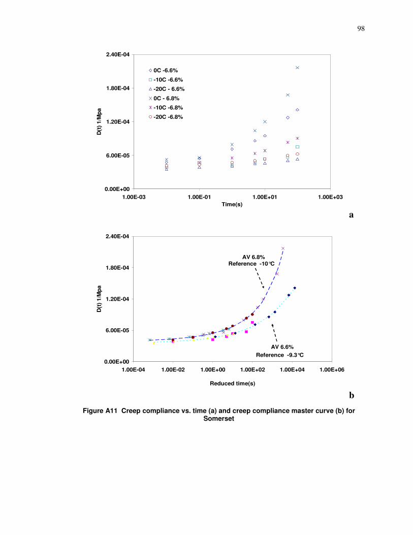
98
0.00E+00
6.00E-05
1.20E-04
1.80E-04
2.40E-04
1.00E-03 1.00E-01 1.00E+01 1.00E+03
Time(s)
D(t
) 1/M
pa
0C -6.6%
-10C -6.6%
-20C - 6.6%
0C - 6.8%
-10C -6.8%
-20C -6.8%
0.00E+00
6.00E-05
1.20E-04
1.80E-04
2.40E-04
1.00E-04 1.00E-02 1.00E+00 1.00E+02 1.00E+04 1.00E+06
Reduced time(s)
D(t
) 1/M
pa
Reference -9.3°C
AV 6.6%
AV 6.8%Reference -10°C
Figure A11 Creep compliance vs. time (a) and creep compliance master curve (b) for Somerset
a
b

99
y = -0.0015x2 - 0.1715x - 1.5646
R2 = 1
y = -0.0079x2 - 0.3235x - 2.3222
R2 = 1
-2.5
-2
-1.5
-1
-0.5
0
0.5
1
1.5
-21 -16 -11 -6 -1 4
Temperature (C)
Lo
g s
hif
t fa
cto
r
AV % = 6.6
AV % = 6.3
2.00E-05
4.00E-05
6.00E-05
8.00E-05
1.00E-04
1.20E-04
1.40E-04
1.60E-04
1.00E-04 1.00E-02 1.00E+00 1.00E+02
Reduced Time(s)
D(t
) 1/M
pa
6.80%
6.60%
Average
Reference -10°C
Figure A12 Shift factor curve (a) and creep compliance master curve at -10°C (b) for Somerset
a
b

100
0.00E+00
6.00E-05
1.20E-04
1.80E-04
2.40E-04
1.00E-03 1.00E-01 1.00E+01 1.00E+03
Time(s)
D(t
) 1/M
pa
0C -8.9%
-10C -8.9%
-20C - 8.9%
0C - 9%
-10C -9%
-20C -9%
0.00E+00
6.00E-05
1.20E-04
1.80E-04
2.40E-04
1.00E-04 1.00E-02 1.00E+00 1.00E+02 1.00E+04
Reduced time(s)
D(t
) 1/M
pa
Reference -10°C
AV 9%
AV 6.8%
Reference -10°C
Figure A13 Creep compliance vs. time (a) and creep compliance master curve (b) for Tioga
a
b

101
y = -0.003x2 - 0.1886x - 1.3585
R2 = 1
y = -0.0031x2 - 0.2187x - 1.8735
R2 = 1
-2.5
-2
-1.5
-1
-0.5
0
0.5
1
1.5
-21 -16 -11 -6 -1 4
Temperature (C)
Lo
g s
hif
t fa
cto
r
AV % = 9
AV % = 8.9
0.00004
0.00005
0.00006
0.00007
0.00008
0.00009
0.0001
0.00011
0.00012
1.00E-05 1.00E-03 1.00E-01 1.00E+01 1.00E+03
Reduced Time(s)
D(t
) 1
/Mp
a
8.90%
9%
Average
Reference -10°C
Figure A14 Shift factor curve (a) and creep compliance master curve at -10°C (b) for Tioga
b
a

102
0.00E+00
5.00E-05
1.00E-04
1.50E-04
2.00E-04
2.50E-04
3.00E-04
3.50E-04
1.00E-03 1.00E-01 1.00E+01 1.00E+03
Time(s)
D(t
) 1/M
pa
0C-6.7%
-10c -6.7%
-20c - 6.7%
0C - 7.5%
-10C - 7.5%
-20C - 7.5%
0C - 7.2%
-10c -7.2%
-20C - 7.2%
0C - 6.6%
-10C - 6.6%
-20C - 6.6%
0.00E+00
5.00E-05
1.00E-04
1.50E-04
2.00E-04
2.50E-04
3.00E-04
3.50E-04
1.00E-04 1.00E-02 1.00E+00 1.00E+02 1.00E+04
Reduced time(s)
D(t
) 1/M
pa
AV 6.6%
Ref -10.6°C
AV 7.5%
Ref -10°C
AV 7.2%
Ref -9.7°C
AV 6.7%
Ref -9.6°C
Figure A14 Creep compliance vs. time (a) and creep compliance master curve (b) for Warren
a
b

103
y = -0.0012x2 - 0.1417x - 1.2978
R2 = 1
y = -0.0001x2 - 0.1816x - 1.7486
R2 = 1
y = -0.0004x2 - 0.1864x - 1.9295
R2 = 1
y = -0.0023x2 - 0.2156x - 1.856
R2 = 1
-2.5
-2
-1.5
-1
-0.5
0
0.5
1
1.5
2
-24 -19 -14 -9 -4 1
Temperature (C)
Lo
g s
hif
t fa
cto
r
AV 7.5%
AV 7.2%
AV 6.6%
AV 6.7%
3.00E-05
8.00E-05
1.30E-04
1.80E-04
2.30E-04
2.80E-04
1.00E-05 1.00E-03 1.00E-01 1.00E+01 1.00E+03
Reduced Time(s)
D(t
) 1/M
pa
7.50%
6.60%
Average
7.20%
6.70%
Reference -10°C
Figure A16 Shift factor curve (a) and creep compliance master curve at -10°C (b) for Warren
a
b

104
Table A1 Sigmoidal coefficients for the SISSI sites
SISSI Site
Blair Delaware Mercer East Mercer West
6.90% 6.50% 6.30% 6.80% 7.20% 7.60% 6.60% 6.30%
a1 -1.62 5.18 -2.85 4.36 7.89 7.92 -0.32 -2.60
a2 -7.94 -25.12 -5.72 -31.96 -29.07 -29.07 -10.43 -5.92
a3 2.61 2.57 3.46 3.64 2.37 2.36 2.58 3.18
a4 0.93 1.93 0.49 2.04 2.87 2.93 0.96 1.15
a5 2.10 3.74 1.64 4.30 4.64 4.45 2.18 1.39
a6 -0.68 -0.46 -1.03 -0.72 -0.40 -0.37 -0.42 -0.54
SISSI Site
Perry Somerset Tioga Warren
6.50% 6.70% 6.80% 6.60% 9% 8.90% 7.50% 6.60% 7.20% 6.70%
a1 -3.48 -1.70 -0.22 -3.08 1.70 0.04 -2.18 11.28 10.06 16.09
a2 -4.09 -7.33 -10.78 -4.50 -16.55 -12.81 -5.59 -41.58 -40.18 -50.03
a3 3.73 2.62 2.57 3.28 2.71 2.93 2.63 2.67 2.80 2.45
a4 0.61 0.84 0.99 1.03 1.26 1.05 0.98 2.57 2.38 4.52
a5 0.75 2.06 2.32 1.24 3.06 2.61 1.60 4.32 4.11 4.86
a6 -0.76 -0.63 -0.49 -0.53 -0.45 -0.45 -0.61 -0.36 -0.37 -0.29

105
Appendix B
Results of 240s BBR tests on SISSI mixtures
0
200
400
600
800
1000
1200
1 10 100 1000
Time(s)
S(t) M
pa
-22C Blair1
-12C Blair 1
-5C Blair 1
-22C Blair 2
-12C Blair 2
-5C Blair 2
10
260
510
760
1010
1.00E-01 1.00E+00 1.00E+01 1.00E+02 1.00E+03 1.00E+04
Reduced time (s)
S(t
) M
pa
Blair -replicate 2
reference -11.92°C
Blair -replicate 1
reference -11.9°C
Figure B1 Creep stiffness vs. time (a) and creep stiffness master curve (b) for Blair
a
b

106
y = -0.131x - 1.5298
R2 = 0.9994
y = -0.1244x - 1.45
R2 = 0.9994
-1
-0.5
0
0.5
1
1.5
2
-25 -20 -15 -10 -5 0
Temperature (C)
Lo
g s
hif
t fa
cto
r
Blair -replicate 2
Blair -replicate 1
Figure B2 Shift factor curve) for Blair

107
0
200
400
600
800
1000
1200
1400
1 10 100 1000
Time(s)
S(t
) M
pa
-22C Delaware 1
-12C Delaware 1
-5C Delaware 1
-22C Delaware 2
-12C Delaware 2
-5C Delaware 2
10
210
410
610
810
1010
0.1 1 10 100 1000 10000
Reduced time (s)
S(t
) M
pa
Delaware -replicate 1
reference -12.07°C
Delaware - replicate 2
reference -12.05°C
Figure B3 Creep stiffness vs. time (a) and creep stiffness master curve (b) for Delaware
a
b

108
y = -0.1338x - 1.5835
R2 = 0.9996
y = -0.1114x - 1.336
R2 = 0.9999
-1.5
-1
-0.5
0
0.5
1
1.5
2
-25 -20 -15 -10 -5 0
Temperature (C)
Lo
g s
hif
t fa
cto
r
Delaware -replicate 2
Delaware -replicate 1
Figure B4 Shift factor curve for Delaware

109
0
200
400
600
800
1000
1200
1 10 100 1000
Time(s)
S(t
) M
pa
-22C ME 1
-12C ME 1
-5C ME 1
-22C ME 2
-12C ME 2
-5C ME 2
10
260
510
760
1010
1260
0.1 1 10 100 1000 10000
Reduced time (s)
S(t
) M
pa
ME -replicate 1
reference -11.7°C
ME -replicate 2
reference -11.6°C
Figure B5 Creep stiffness vs. time (a) and creep stiffness master curve (b) for Mercer East (ME)
a
b

110
y = -0.1346x - 1.4796
R2 = 0.9961
y = -0.1344x - 1.4908
R2 = 0.9962
-1
-0.5
0
0.5
1
1.5
2
-25 -20 -15 -10 -5 0
Temperature (C)
Lo
g s
hif
t fa
cto
r
ME -replicate 2
ME -replicate 1
Figure B6 Shift factor curve for Mercer East

111
0
200
400
600
800
1000
1200
1 10 100 1000
Time(s)
S(t
) M
pa
-22C MW 1
-12C MW 1
-5C MW 1
-22CMW 2
-12C MW 2
-5C MW 2
10
260
510
760
1010
1260
0.1 1 10 100 1000 10000
Reduced time (s)
S(t
) M
pa
MW -replicate 2
reference -11.88°C
MW -replicate 1
reference -11.93°C
Figure B7 Creep stiffness vs. time (a) and creep stiffness master curve (b) for Mercer West (MW)
a
b

112
y = -0.1183x - 1.2965
R2 = 0.9914
y = -0.1418x - 1.5273
R2 = 0.9863
-1
-0.5
0
0.5
1
1.5
2
-25 -20 -15 -10 -5 0
Temperature (C)
Lo
g s
hif
t fa
cto
r
MW -replicate 1
MW -replicate 2
Figure B8 Shift factor curve for Mercer West

113
0
100
200
300
400
500
600
700
800
900
1 10 100 1000
Time(s)
S(t
) M
pa
-22C Perry 1
-12C Perry 1
-5C Perry 1
-22C Perry 2
-12C Perry 2
-5C Perry 2
10
210
410
610
810
1010
0.1 1 10 100 1000 10000
Reduced time (s)
S(t
) M
pa
Perry -replicate 2
reference -11.96°C
Perry -replicate 1
reference -11.99°C
Figure B9 Creep stiffness vs. time (a) and creep stiffness master curve (b) for Perry
a
b

114
y = -0.1204x - 1.4218
R2 = 0.9998
y = -0.1227x - 1.3756
R2 = 0.9939-1
-0.5
0
0.5
1
1.5
2
-25 -20 -15 -10 -5 0
Temperature (C)
Lo
g s
hif
t fa
cto
rPerry -replicate 1
Perry -replicate 2
Figure B10 Shift factor curve for Perry

115
0
200
400
600
800
1000
1200
0.1 1 10 100 1000
Time(s)
S(t
) M
pa
-22C Somerset 1
-12CSomerset 1
-5C Somerset 1
-22C Somerset 2
-12C Somerset 2
-5C Somerset 2
10
260
510
760
1010
0.1 1 10 100 1000 10000
Reduced time (s)
S(t
) M
pa
Somerset -replicate 2
reference -11.88°C
Somerset -replicate 1
reference -11.87°C
Figure B11 Creep stiffness vs. time (a) and creep stiffness master curve (b) for Somerset
a
b

116
y = -0.1285x - 1.4434
R2 = 0.9958
y = -0.1337x - 1.5604
R2 = 0.9996
-1
-0.5
0
0.5
1
1.5
2
-25 -20 -15 -10 -5 0
Temperature (C)
Lo
g s
hif
t fa
cto
r
Somerset -replicate
2
Somerset -replicate 1
Figure B12 Shift factor curve for Somerset

117
0
200
400
600
800
1000
1200
1 10 100 1000
Time(s)
S(t
) M
pa
-22C Warren1
-12C Warren 1
-5C Warren 1
-22C Warren 2
-12C Warren 2
-5C Warren 2
10
210
410
610
810
1010
0.1 1 10 100 1000 10000
Reduced time (s)
S(t
) M
pa
Warren -replicate 1
reference -12.05°C
Warren -replicate 2
reference -11.99°C
Figure B3 Creep stiffness vs. time (a) and creep stiffness master curve (b) for Warren
a
b

118
y = -0.1269x - 1.4083
R2 = 0.9919
y = -0.1395x - 1.6283
R2 = 0.9986
-1.5
-1
-0.5
0
0.5
1
1.5
2
-25 -20 -15 -10 -5 0
Temperature (C)
Lo
g s
hif
t fa
cto
r
Warren -replicate
1
Warren -replicate
Figure B4 Shift factor curve) for Warren

119
Appendix C
M-values for 240s and 2hr BBR tests on SISSI binders
Table C1 M-values for 240s and 2hr BBR tests on SISSI binders
240s test 2hr test
SISSI Site m-value @ 60s
m-value @ 60s
Temperature (°C) Temperature (°C)
-22 -12 -5 -22 -12 -5
Warren -replicate 1 0.242 0.337 0.42 0.227 0.32 0.412
Warren -replicate 2 0.24 0.327 0.432 0.227 0.322 0.411
Blair -replicate 1 0.225 0.333 0.42 0.211 0.324 0.422
Blair-replicate 2 0.212 0.312 0.398 0.204 0.299 0.399
Somerset - replicate 1 0.241 0.341 0.433 0.231 0.33 0.432
Somerset -replicate 2 0.242 0.328 0.432 0.231 0.327 0.429
Mercer East -replicate 1 0.251 0.377 0.502 0.255 0.37 0.482
Mercer East-replicate 2 0.252 0.367 0.49 0.242 0.367 0.497
Mercer West- replicate 1 0.187 0.289 0.36 0.214 0.281 0.365
Mercer West - replicate 2 0.222 0.293 0.379 0.217 0.293 0.373
Perry - replicate 1 0.25 0.319 0.41 0.24 0.319 0.419
Perry - replicate 2 0.257 0.357 0.441 0.243 0.35 0.466
Delaware - replicate 1 0.228 0.294 0.378 0.19 0.289 0.389
Delaware - replicate 2 0.202 0.298 0.384 0.201 0.288 0.378