EVALUATION OF INTEGER WEIGHTING FOR THE … OF INTEGER WEIGHTING FOR THE 1997 CENSUS OF AGRICULTURE, ... Wade for the Mapinfo tutorial, and Phil Kott for …

i

EVALUATION OF INTEGER WEIGHTING FOR THE 1997 CENSUS OF AGRICULTURE,by Wendy Scholetzky, Sampling and Estimation Research Section, Research Division, NationalAgricultural Statistics Service, U.S. Department of Agriculture, Washington, DC 20250-2000, January2000, Report No. RD-00-01.

ABSTRACT

The census of agriculture is an important source of statistics about the Nation’s agricultural production andprovides consistent, comparable data at the county, state, and national levels. Each census record hasweights which are used to produce totals for the entire population. The process of rounding weights tointeger values has been in place for the last several censuses. When a record’s weight is rounded to aninteger value, the totals represented by that record may or may not change dramatically. These changesmay or may not become negligible when producing totals at the state or county level. This reportcompares totals calculated with the noninteger weights to the published totals (calculated with the integerweights) for the 1997 Census of Agriculture, evaluates how different these totals are, and examines howthe differences relate to the standard error. The analysis examines a number of characteristics at both thestate and county levels. The report also examines another weighting approach where the nonintegerweights are applied to the record and the weighted data values are rounded at the record level. Thedifference between totals produced with these values and the noninteger weights is calculated andcompared to the above differences.

The reasons for rounding weights, to ease data review procedures and to ensure that publication totalsadd, are legitimate concerns. The author asserts that it is possible to address these two concerns andimprove the totals produced when NASS revamps the census processing system for the 2002 census.

KEY WORDS

1997 Census of Agriculture; Integer weight; Noninteger weight; t-value; Percent difference.

This paper was prepared for limited distribution to the research community outside the U.S. Department of Agriculture.

ACKNOWLEDGMENTS

The author would like to thank Dale Atkinson for his guidance in the development of this report, GailWade for the Mapinfo tutorial, and Phil Kott for providing the standard error methodology. A specialthanks to Chadd Crouse for his tremendous assistance throughout the entire project.

ii

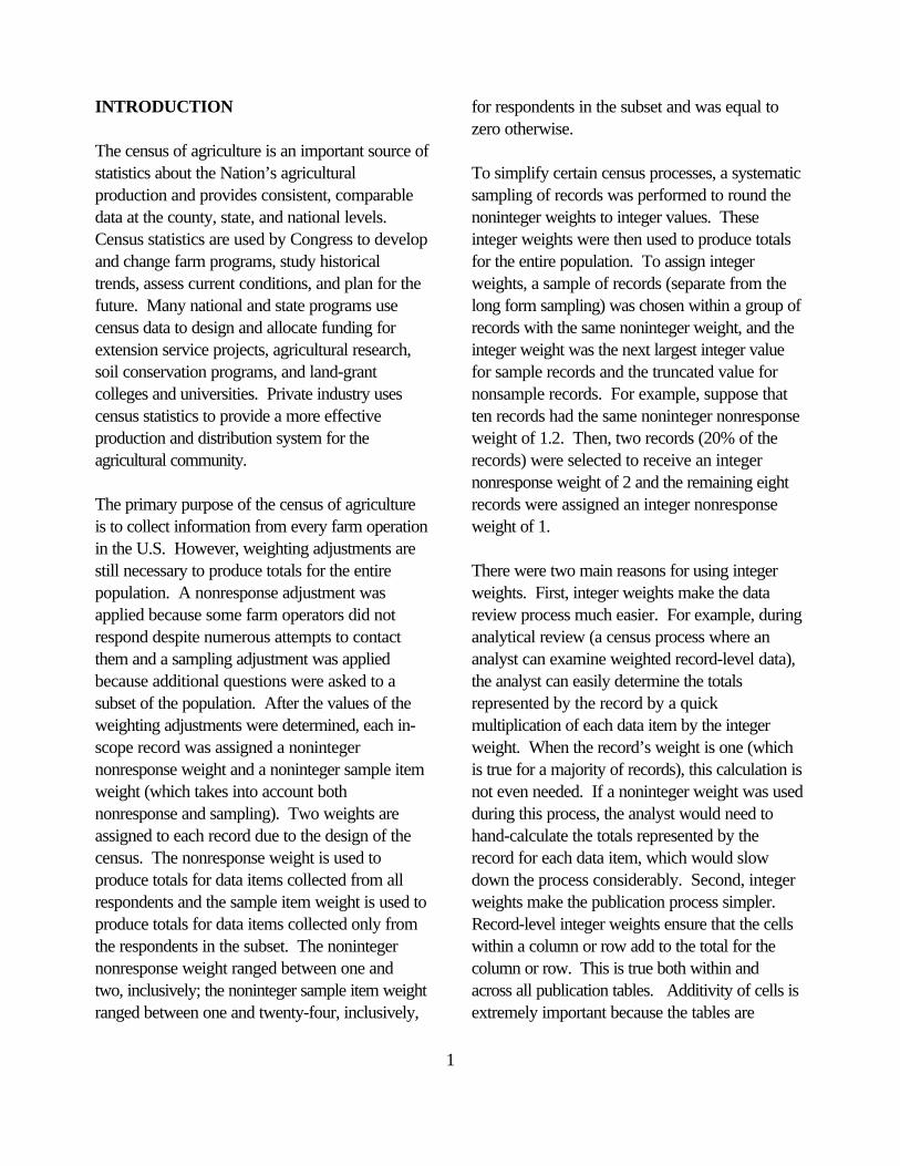
TABLE OF CONTENTS

ABSTRACT . . . . . . . . . . . . . . . . . . . . . . . . . . . . . . . . . . . . . . . . . . . . . . . . . . . . . . . . . . . . . . . . . . . . i

SUMMARY . . . . . . . . . . . . . . . . . . . . . . . . . . . . . . . . . . . . . . . . . . . . . . . . . . . . . . . . . . . . . . . . . . . iii

INTRODUCTION . . . . . . . . . . . . . . . . . . . . . . . . . . . . . . . . . . . . . . . . . . . . . . . . . . . . . . . . . . . . . . 1

BACKGROUND . . . . . . . . . . . . . . . . . . . . . . . . . . . . . . . . . . . . . . . . . . . . . . . . . . . . . . . . . . . . . . . 2

RESULTS AND DISCUSSION . . . . . . . . . . . . . . . . . . . . . . . . . . . . . . . . . . . . . . . . . . . . . . . . . . . 5

Differences in Totals at the State Level . . . . . . . . . . . . . . . . . . . . . . . . . . . . . . . . . . . . . . . . . . 6

Differences in Totals at the County Level . . . . . . . . . . . . . . . . . . . . . . . . . . . . . . . . . . . . . . . . 8

An Alternative Weighting Procedure . . . . . . . . . . . . . . . . . . . . . . . . . . . . . . . . . . . . . . . . . . 14

RECOMMENDATIONS . . . . . . . . . . . . . . . . . . . . . . . . . . . . . . . . . . . . . . . . . . . . . . . . . . . . . . . . 15

REFERENCES . . . . . . . . . . . . . . . . . . . . . . . . . . . . . . . . . . . . . . . . . . . . . . . . . . . . . . . . . . . . . . . 16

APPENDIX A . . . . . . . . . . . . . . . . . . . . . . . . . . . . . . . . . . . . . . . . . . . . . . . . . . . . . . . . . . . . . . . . 17

APPENDIX B . . . . . . . . . . . . . . . . . . . . . . . . . . . . . . . . . . . . . . . . . . . . . . . . . . . . . . . . . . . . . . . . 18

APPENDIX C . . . . . . . . . . . . . . . . . . . . . . . . . . . . . . . . . . . . . . . . . . . . . . . . . . . . . . . . . . . . . . . . 21

APPENDIX D . . . . . . . . . . . . . . . . . . . . . . . . . . . . . . . . . . . . . . . . . . . . . . . . . . . . . . . . . . . . . . . . 44

APPENDIX E . . . . . . . . . . . . . . . . . . . . . . . . . . . . . . . . . . . . . . . . . . . . . . . . . . . . . . . . . . . . . . . . 50

iii

SUMMARY

The census of agriculture is an important source of statistics about the Nation’s agricultural production andprovides consistent, comparable data at the county, state, and national levels. Each census record has twoweights which are used to produce totals for the entire population. The first weight is the nonresponseweight which accounts for farm operators who did not respond to the census despite numerous attempts tocontact them. The second weight is the sample item weight which accounts for both nonresponse andsubsampling for data items that are only asked on the long form.

The process of rounding weights to integer values has been in place for the last several censuses. When arecord’s weight is rounded to an integer value, the totals represented by that record may or may notchange dramatically. These changes may or may not become negligible when producing totals at the stateor county level. The definition of what a person considers negligible is open to debate. Rather than roundthe noninteger weights to integer values, another possible approach is to apply the noninteger weights tothe record and round the weighted data values at the record level. Thus, the operation’s rounded-weighteddata values are used to produce the totals for the entire population. With this approach, alternativemethodology would have to be used for characteristics such as number of farms and demographic data.

This report compares totals calculated with the noninteger weights to the published totals (calculated withthe integer weights) for the 1997 Census of Agriculture, evaluates how different these totals are, andexamines how the differences relate to the standard error. The report also compares these differences tothe difference between totals produced with the noninteger weights and the record’s rounded-weighteddata values. The analysis examines a number of characteristics at both the state and county levels.

The reasons for rounding weights, to ease data review procedures and to ensure that publication totalsadd, are legitimate concerns. The author asserts that it is possible to address these two concerns andimprove the totals produced when NASS revamps the census processing system for the 2002 census. Inreference to data review procedures, one argument for using the integer weights is that one can “easily”obtain weighted totals for a record of interest during the data review phase. In the 1997 system, thiswould be accomplished by multiplying the integer weight by each record’s data value of interest. Thus, thismanual computation is easier if the nonresponse weight is 2 rather than 1.7. However, for the 2002system, the computer can and should perform this calculation. With this improvement, the value of theweight is no longer relevant. In reference to the concern that the publication totals add, a combination ofthe integer weights and the record’s rounded-weighted data values should be used. The integer weightsshould be used to produce totals for indicator and categorical variables and for any question where thedata values are small for most farms. The record’s rounded-weighted data values should be used toproduce totals for all other characteristics. With this improvement, the integer sample item weight is nolonger necessary unless the 2002 long form contains a question that requires it. The 1997 long formcontained no such item. Once the 2002 long form is finalized, the questions will need to be evaluated todetermine whether the integer sample item weight is needed.

1

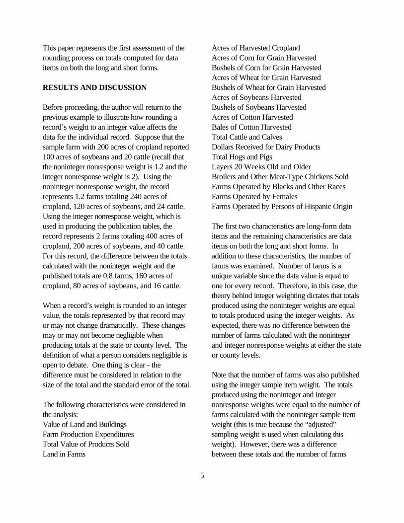
INTRODUCTION

The census of agriculture is an important source ofstatistics about the Nation’s agriculturalproduction and provides consistent, comparabledata at the county, state, and national levels. Census statistics are used by Congress to developand change farm programs, study historicaltrends, assess current conditions, and plan for thefuture. Many national and state programs usecensus data to design and allocate funding forextension service projects, agricultural research,soil conservation programs, and land-grantcolleges and universities. Private industry usescensus statistics to provide a more effectiveproduction and distribution system for theagricultural community.

The primary purpose of the census of agricultureis to collect information from every farm operationin the U.S. However, weighting adjustments arestill necessary to produce totals for the entirepopulation. A nonresponse adjustment wasapplied because some farm operators did notrespond despite numerous attempts to contactthem and a sampling adjustment was appliedbecause additional questions were asked to asubset of the population. After the values of theweighting adjustments were determined, each in-scope record was assigned a nonintegernonresponse weight and a noninteger sample itemweight (which takes into account bothnonresponse and sampling). Two weights areassigned to each record due to the design of thecensus. The nonresponse weight is used toproduce totals for data items collected from allrespondents and the sample item weight is used toproduce totals for data items collected only fromthe respondents in the subset. The nonintegernonresponse weight ranged between one andtwo, inclusively; the noninteger sample item weightranged between one and twenty-four, inclusively,

for respondents in the subset and was equal tozero otherwise.

To simplify certain census processes, a systematicsampling of records was performed to round thenoninteger weights to integer values. Theseinteger weights were then used to produce totalsfor the entire population. To assign integerweights, a sample of records (separate from thelong form sampling) was chosen within a group ofrecords with the same noninteger weight, and theinteger weight was the next largest integer valuefor sample records and the truncated value fornonsample records. For example, suppose thatten records had the same noninteger nonresponseweight of 1.2. Then, two records (20% of therecords) were selected to receive an integernonresponse weight of 2 and the remaining eightrecords were assigned an integer nonresponseweight of 1.

There were two main reasons for using integerweights. First, integer weights make the datareview process much easier. For example, duringanalytical review (a census process where ananalyst can examine weighted record-level data),the analyst can easily determine the totalsrepresented by the record by a quickmultiplication of each data item by the integerweight. When the record’s weight is one (whichis true for a majority of records), this calculation isnot even needed. If a noninteger weight was usedduring this process, the analyst would need tohand-calculate the totals represented by therecord for each data item, which would slowdown the process considerably. Second, integerweights make the publication process simpler. Record-level integer weights ensure that the cellswithin a column or row add to the total for thecolumn or row. This is true both within andacross all publication tables. Additivity of cells isextremely important because the tables are

2

broken into extremely detailed cells for variouscharacteristics and a tremendous number of tablesare produced during the publication process (onevolume for each state plus one for the UnitedStates). If noninteger weights were used duringthis process, each cell would need to be roundedwhich does not guarantee additivity of cells. Forexample, noninteger weights could result in thefollowing scenario...there are 100 farms with lessthan 1,000 acres and 50 farms with 1,000 acresor more, but the total number of farms is equal to151.

Totals produced using the integer weights areunbiased estimates of totals produced using thenoninteger weights. Therefore, in a perfect world,these two values are equal. However, variousfactors may affect the results. One possibility isthat the records chosen to receive an integernonresponse weight of 2 may not be arepresentative sample. Returning to the previousexample, suppose that the two sample recordshad 100 and 200 acres of cropland and theaverage of the eight nonsample records was 400acres. This would result in 3,800 total acres usingthe integer weights compared to 4,200 total acresusing the noninteger weights. Another possibilityis that the distribution of the data is skewed,which is common with agricultural data. Formany characteristics, the distribution is skewed tothe right since there are a lot of farms with smallervalues and a few farms with larger values. Therefore, the probability of assigning an integerweight of 2 to farms below the average is greaterthan ½ and the probability of assigning an integerweight of 2 to farms above the average is lessthan ½. (If the data were normally distributed,both probabilities would equal ½.) In this case,there is a tendency for the integer weights tounderestimate the total, especially for smallgeographic areas (i.e., county-level data).

Note that the process of rounding weights affectsthe sample item weights and the nonresponseweights differently. First, since the sample itemweights are larger in magnitude than thenonresponse weights, there is less of an effect onthe totals. Second, since the integer sample itemweights are equal to one less frequently than theinteger nonresponse weights, more recordscontribute to the adjustment. (The averagenoninteger sample item weight is 3.819 and theaverage noninteger nonresponse weight is 1.139.) In other words, records with an integernonresponse weight of one do not represent anonrespondent.

This report compares totals calculated with thenoninteger weights to the published totals(calculated with the integer weights) for the 1997Census of Agriculture, evaluates how differentthese totals are, and examines how the differencesrelate to the standard error. The author discussestotals for a number of characteristics at both thestate and county levels. The author also examinesanother possible approach where the nonintegerweights are applied to the record and theweighted data values are rounded at the recordlevel (referred to as record’s rounded-weighteddata values). The difference between totalsproduced with the noninteger weights and therecord’s rounded-weighted data values arecalculated and compared to the abovedifferences.

BACKGROUND

For more than 150 years, there has been a censusof agriculture. The first agriculture census wastaken in 1840. From 1840 to 1950, theagriculture census was taken as part of thedecennial census. A separate mid-decade censusof agriculture was conducted in 1925, 1935, and1945. From 1954 to 1974, a census of

3

agriculture was taken for the years ending in 4 and9. In 1976, Congress authorized the census ofagriculture to be taken for 1978 and 1982 toadjust the data reference year so that it coincidedwith other economic censuses. This adjustment intiming established the agriculture census on a 5-year cycle collecting data for years ending in 2and 7. Beginning with the 1997 Census ofAgriculture, responsibility was transferred fromthe U.S. Department of Commerce, Bureau of theCensus to the U.S. Department of Agriculture,National Agricultural Statistics Service.

To reduce data collection costs for the 1997Census of Agriculture, a screening operation wasconducted by mail and telephone to survey about500,000 records identified as having a lowprobability of being a farm. Records with noagricultural activity were removed from the censusmail list. In December 1997, approximately3,155,000 records were mailed a censusquestionnaire and about 34,000 tagged records(farms which were abnormal, multi-unit, in theARMS survey, or identified by a State StatisticalOffice (SSO) for special handling) were givendirectly to the SSOs for data collection. A thankyou/reminder card was mailed to everyone inearly January 1998. Nonrespondents, except for1992 census nonrespondents and large farms,were then sent two follow-up mailings in mid-February and late March. Telephone calls weremade in early February to nonrespondents whowere also 1992 census nonrespondents and inearly March to nonrespondents classified as largefarms. From early April until late May, telephonecalls were made to all remaining nonrespondentsto encourage them to respond to the census andto ensure at least a 75% response rate within eachcounty.

To reduce respondent burden, the census usedtwo forms - a long form and a short form. The

long form is the same as the short form butcontains additional questions on the usage offertilizers and chemicals, farm productionexpenditures, value of machinery and equipment,value of land and buildings, and farm relatedincome. All records classified as certainty (taggedrecords; farms greater than a state-specified levelfor acreage and total value of products sold(TVP); special insert cases such as Christmastrees and maple sap farms; farms in Rhode Island,Alaska, and Hawaii; or records in a county thatcontained fewer than 100 farms in the 1992census) received a long form. A systematicsample was then taken at the county level fromthe remaining noncertainty records to also receivethe long form. The county’s sampling rate wasbased on 1992 farm counts and was either 1-in-1, 1-in-2, 1-in-4, or 1-in-6.

Each census record has two weights which areused to produce totals for the entire population. The first weight is the nonresponse weight whichaccounts for farm operators who did not respondto the census despite numerous attempts tocontact them. Information on farming status forthe nonrespondents was obtained from the 1997Nonresponse Survey. At the end of the censusfollow-up operations, a stratified systematicsample of nonresponse records was selected forthis survey within each state (except for Alaskaand Rhode Island which required a 100%response rate). The strata were formed based onscreener status, TVP, and number of sourcesfrom which the record was obtained during thedevelopment of the mail list. From the survey, thenumber of census nonrespondents that operatedfarms was estimated at the stratum level in eachstate, and these estimates were allocated to thecounty level. Within each county/stratum, thenoninteger nonresponse weight was calculated asthe total number of farms (respondents thatoperated farms plus the estimated number of

4

nonrespondents that operated farms) divided bythe number of respondents that operated farms. Strata were collapsed if the nonintegernonresponse weight was greater than two, toprevent an individual record from representingmore than one nonrespondent. The nonintegernonresponse weight for each farm was thenrounded to either one or two. All farms classifiedas large based on total acreage, TVP, commodityproduction, or certain characteristics (i.e., value ofland and buildings, value of machinery andequipment, farm-related income, number ofworkers, etc.); all tagged records; and all farmswith uncommon commodities were assigned anonresponse weight of one. This was becausethese records either required a 100% responserate or could not represent a nonrespondent. From the remaining records, a systematic sampleof records was selected within eachcounty/stratum for the integer rounding; the integernonresponse weight was two for sample recordsand one for nonsample records.

The second weight is the sample item weightwhich accounts for both nonresponse andsubsampling for data items that are only asked onthe long form. Operationally, this weight wasreferred to as the sample weight; the author hasexpanded the name to avoid confusion with thestandard definition of a sample weight. Thesample item weight was calculated by multiplyingthe noninteger nonresponse weight by the“adjusted” sampling weight (the “adjusted”sampling weight uses only respondents thatoperated farms). Certainty farms were alwaysassigned an adjusted sampling weight of one. Thenoncertainty farms were stratified based on TVP,total acreage, and Standard IndustrialClassification code. Within each stratum, theadjusted sampling weight was calculated as thesum of the noninteger nonresponse weights fornoncertainty farms (long-form noncertainty farms

plus short-form noncertainty farms) divided by thesum of the noninteger nonresponse weights forlong-form noncertainty farms. Strata werecollapsed if the adjusted sampling weight wasgreater than twice the original sampling weight orif the sum of the noninteger nonresponse weightsfor long-form noncertainty records was less than10. The noninteger sample item weight for eachnoncertainty farm was then rounded to an integervalue. A systematic sample of records wasselected within each county/nonresponsestratum/sample stratum for the integer rounding;the integer sample item weight was the nextlargest integer value for sample records and thetruncated value for nonsample records.

As previously stated, the purpose of thenonresponse and sample item weights is toproduce totals for the entire population (for moredetails on the weighting adjustments, refer to thememoranda written by Swan and Scholetzky). The nonresponse weight is used when generatingtotals for data items collected from allrespondents (the question appears on both thelong and short forms) and the sample item weightis used when generating totals for data itemscollected from a subset of all respondents (thequestion appears only on the long form).

The process of rounding weights to integer valueshas been in place for the last several censuses. In1993, research was done to examine how thisprocess affects the aggregates by analyzingcounty-level totals for three long-formcharacteristics in two states (Kraus-Winters,1993). Although that paper concentrated moreon examining the effect on the variance of thetotals, the authors concluded “the results indicatethat minor discrepancies at the strata level due tosystematic rounding accumulate to sizabledifferences at the published level for some farmcharacteristics.”

5

This paper represents the first assessment of therounding process on totals computed for dataitems on both the long and short forms.

RESULTS AND DISCUSSION

Before proceeding, the author will return to theprevious example to illustrate how rounding arecord’s weight to an integer value affects thedata for the individual record. Suppose that thesample farm with 200 acres of cropland reported100 acres of soybeans and 20 cattle (recall thatthe noninteger nonresponse weight is 1.2 and theinteger nonresponse weight is 2). Using thenoninteger nonresponse weight, the recordrepresents 1.2 farms totaling 240 acres ofcropland, 120 acres of soybeans, and 24 cattle. Using the integer nonresponse weight, which isused in producing the publication tables, therecord represents 2 farms totaling 400 acres ofcropland, 200 acres of soybeans, and 40 cattle. For this record, the difference between the totalscalculated with the noninteger weight and thepublished totals are 0.8 farms, 160 acres ofcropland, 80 acres of soybeans, and 16 cattle.

When a record’s weight is rounded to an integervalue, the totals represented by that record mayor may not change dramatically. These changesmay or may not become negligible whenproducing totals at the state or county level. Thedefinition of what a person considers negligible isopen to debate. One thing is clear - thedifference must be considered in relation to thesize of the total and the standard error of the total.

The following characteristics were considered inthe analysis: Value of Land and BuildingsFarm Production ExpendituresTotal Value of Products SoldLand in Farms

Acres of Harvested CroplandAcres of Corn for Grain HarvestedBushels of Corn for Grain HarvestedAcres of Wheat for Grain HarvestedBushels of Wheat for Grain HarvestedAcres of Soybeans HarvestedBushels of Soybeans HarvestedAcres of Cotton HarvestedBales of Cotton HarvestedTotal Cattle and CalvesDollars Received for Dairy ProductsTotal Hogs and Pigs Layers 20 Weeks Old and OlderBroilers and Other Meat-Type Chickens SoldFarms Operated by Blacks and Other RacesFarms Operated by FemalesFarms Operated by Persons of Hispanic Origin

The first two characteristics are long-form dataitems and the remaining characteristics are dataitems on both the long and short forms. Inaddition to these characteristics, the number offarms was examined. Number of farms is aunique variable since the data value is equal toone for every record. Therefore, in this case, thetheory behind integer weighting dictates that totalsproduced using the noninteger weights are equalto totals produced using the integer weights. Asexpected, there was no difference between thenumber of farms calculated with the nonintegerand integer nonresponse weights at either the stateor county levels.

Note that the number of farms was also publishedusing the integer sample item weight. The totalsproduced using the noninteger and integernonresponse weights were equal to the number offarms calculated with the noninteger sample itemweight (this is true because the “adjusted”sampling weight is used when calculating thisweight). However, there was a differencebetween these totals and the number of farms

6

calculated with the integer sample item weight. The author is not sure why this resulted; it couldhave occurred because of the small number offarms within a county/nonresponse stratum/samplestratum or because the rounding methodologywasn’t consistent within the weighting program. Whatever the reason, the differences are not largecompared to the number of farms in the state. The three largest differences were 53 farms inNew York, 35 farms in West Virginia, and 25farms in Maryland. At the county level, thedifferences were small. But, both the state andcounty differences could be troublesome to a datauser. One example of this appears on page C-16of Table F in the United States publication, wherethe two totals are adjacent to each other. A datauser might improperly conclude that thesedifferences were an error.

In this report, the author refers to the totalscalculated with the integer weights as thepublished totals. This terminology is not literal;totals for the above characteristics do not appearin the census publication when the total wassuppressed due to confidentiality

concerns or the commodity was not published forthat state. The analysis done for this reportconcentrated more on comparing the county-leveltotals than the state-level totals. This is becausethe differences are not as predominant at thestate-level and because the primary purpose ofthe census is to produce county-level totals. Thereport first presents a brief discussion of the state-level totals and then a more in-depth analysis ofthe county-level totals.

Differences in Totals at the State Level

The t-value was used to evaluate the differencebetween the published and noninteger totals at thestate level. A t-value was determined bysubtracting the noninteger total from the publishedtotal and dividing this quantity by the standarderror of the difference. The standard error wascalculated using the formula described inAppendix A and the t-value was compared to atwo-tailed Student t distribution. When the t-value for a characteristic exceeded the thresholdfor 90% significance, the difference in the state-level totals was defined to be “large.” Table 1lists the states that were determined to have largedifferences for each characteristic.

7

Table 1: State Totals with Statistically Significant Differences

Characteristic States

Value of Land and BuildingsFarm Production ExpendituresTotal Value of Products SoldLand in FarmsAcres of Harvested CroplandAcres of Corn for Grain HarvestedBushels of Corn for Grain HarvestedAcres of Wheat for Grain HarvestedBushels of Wheat for Grain HarvestedAcres of Soybeans HarvestedBushels of Soybeans HarvestedAcres of Cotton HarvestedBales of Cotton HarvestedTotal Cattle and CalvesDollars Received for Dairy ProductsTotal Hogs and PigsLayers 20 Weeks Old and OlderBroilers and Other Meat-Type Chickens SoldFarms Operated by Blacks and Other RacesFarms Operated by FemalesFarms Operated by Persons of Hispanic Origin

CO, KY*, LA, MD*, MI*, MT, NC*, OK**, SC, VTND

AZ**

CA*, GA*, OKAZ*, AR, CT, HI*, ME, NC*, SD*

CO, DE, KS, LA, NH, ND, VT**

DE*, KS, NH, ND, VT**, WY*

IA, MS, NV*, NY**

FL, IA, MS, NV**, NY**

AL, OKNoneMO

MO*, NMKY, VT*, WI

DE, IL*, LA**, MS*, UT, WY*

LA**, NM*, OH, TN**

MD, NH*, PA*, VT*, WIKS**, ME, WI*

AZ*, KY*, NMCO*, GA, HI*, ME, MN*, ND**, SD*

IN, KY*, MD*, MI**, MN*, NM, OH**, OR*, WI*,WY*

* Greater than or equal to a 95% significance level. ** Greater than or equal to a 99% significance level.

There were several situations where the t-valuewas just less than a 90% significance level. Sincestate totals for these are large enough to bepotentially of practical importance, the author alsoconsiders the difference in the state-level totals tobe large for: total value of products sold in SDwith a t-value of 1.631, acres of corn for grainharvested in AR with a t-value of 1.617, acres ofwheat for grain harvested in GA and NE with t-values of 1.627 and 1.611, bushels of wheat forgrain harvested in MI with a t-value of 1.626,acres of soybeans harvested in PA with a t-valueof 1.618, acres of soybeans harvested in PA witha t-value of 1.625, total cattle and calves in FLwith a t-value of 1.632, and total hogs and pigs inAZ with a t-value of 1.644.

Interpretation of the results presented in Table 1depends on the reader. For example, a personmay not be concerned with a significant differencein a state when the characteristic is a smallpercentage of the national total. On the otherhand, another person may be concerned that theprocess of rounding weights results in a significantdifference for any characteristic at the state level. The difference and percent difference can be usedto help evaluate the importance of the statisticalsignificance. The percent difference is computedby subtracting the noninteger total from thepublished total, dividing by the noninteger total,and converting this to a percentage. To illustratethis methodology, the author will discuss twostates which were significant at the 99% level.

8

For acres of corn for grain harvested in Vermont,the difference was -147 acres and the percentdifference was -1.75 percent. For broilers andother meat-type chickens sold in Kansas, thedifference was -3,507 chickens and the percentdifference was -9.10 percent. A listing of allstate/characteristic combinations that arestatistically significant at the 90% level is providedin Appendix B.

Although not specifically presented in a table, itshould be noted that it is possible for a state tohave a large percent difference between thepublished and noninteger totals that is notstatistically significant. For example, for acres ofcorn for grain in Nevada, the difference was 50acres and the percent difference was 14.45 butthe t-value was 0.901. For broilers and othermeat-type chickens sold in Colorado, thedifference was 2,082 and the percent differencewas 21.13 but the t-value was 0.917.

Differences in Totals at the County Level

As stated earlier, a more comprehensive analysiswas performed on totals at the county level. Theanalysis was performed on all 21 characteristicsfor every county in the 48 contiguous states. “Small” counties were identified for eachcharacteristic and excluded from the analysis. Originally, a county was defined as “small” whenthe total for the characteristic was less than 1% ofthe state total. However, this definition resulted ineliminating too many counties in states with a largenumber of counties (i.e., Texas). In order toaccount for the variation in the number of countiesamong states, the concept of “expected countycontribution” was adopted. Expected countycontribution is defined as the multiplicative inverseof the state’s number of counties times the statetotal for the characteristic. So, a county wasdefined as “small” when it contained less than the

expected county contribution. For example, if acounty in Texas contained 20,000 acres ofcotton, then it was considered to be small since20,000 is less than the inverse of the number ofcounties (254-1) times the total number of acres ofcotton in Texas (5,221,561). Using thisprocedure, the definition of a small county fornumber of acres of cotton in Texas was 20,557rather than the original definition of 52,215. Inaddition to the concept of expected countycontribution, for the three demographic variables,a county was determined to be “small” when thecounty’s sum of the integer nonresponse weightswas less than three.

After eliminating small counties from the analysis,two statistics were used to evaluate the differencebetween the published and noninteger totals. First, a t-value was calculated by subtracting thenoninteger total from the published total anddividing this quantity by the standard error of thedifference. Like the state-level analysis, thestandard error was calculated using the formuladescribed in Appendix A, and the t-value wascompared to a two-tailed Student t distribution. When the t-value for a characteristic exceededthe threshold for 90% significance, the differencein the county-level totals was defined to be“large.” Second, a percent difference wascomputed by subtracting the noninteger total fromthe published total, dividing by the nonintegertotal, and converting this to a percentage. Unlikethe t-value, this method did not use a specificcutoff to define a “large” difference in the county-level totals. Instead, the analysis focused oncounties with the largest percent differences foreach characteristic.

Various tables and maps were created in an effortto show the key results of the analysis. Resultsfrom each method are presented as well as resultsfrom combining the methods. While interpretation

9

of these results depends on the reader, the authorhas attempted to present an unbiasedsummarization of the analysis.

Table 2 presents the number of nonsmall countieswith statistically significant differences. For eachcharacteristic, the table shows the number ofnonsmall counties that were significant at the threemost commonly-used levels and the percentage ofstatistically significant nonsmall counties at the90% level.

The three significance levels are shown to give ameasure of how different the published total isfrom the noninteger total. The number of countiesat the 95% and 99% significance levels aresubsets of the previous significance level. Forexample, 100 counties are significant at the 90%level for value of land and buildings; 44 of these100 counties are

significant at the 95% level. The last column, thepercentage with significant differences, is shownto give a measure of the number of differences. This percentage was calculated by dividing thenumber of nonsmall counties that were significantat the 90% level (shown in column three) by thetotal number of nonsmall counties for thecharacteristic (shown in column two) andmultiplying by 100. Farms operated by personsof Hispanic origin had the largest percentage ofsignificant counties and farm productionexpenditures had the smallest. The two long-formcharacteristics performed much better than thecharacteristics collected on both the long andshort forms. This is not surprising since theprocess of rounding weights has less of an effecton the totals as the weight increases, and thesample item weights

Table 2: Number of Nonsmall Counties with Statistically Significant Differences

CharacteristicNumber ofNonsmallCounties

Significance Level % withSignificant

Differences$ 90% $ 95% $ 99%

10


12851033107313071160932885853824849825282276

1170713706362296644

1073643

10023125133126131129111111919637351141131115725130148199

44157771657676565251531713665655309

8783103

135

19111529238

10131142

23191860

282018

7.782.23

11.6510.1810.8614.0614.5813.0113.4710.7211.6413.1212.689.74

15.8515.7215.758.45

20.1913.7930.95

are larger in magnitude than the nonresponseweights.

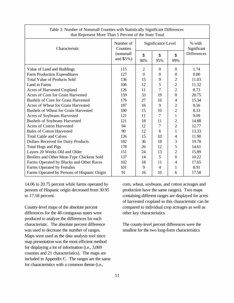
An interesting subset of the counties tallied inTable 2 is the collection of those counties thatrepresented a substantial percentage of the statetotal. Table 3 provides the number of nonsmallcounties with statistically significant differences,where the county represented more than 5percent of the state total. Again, for eachcharacteristic, the table shows the number ofnonsmall counties that were significant at the threemost commonly-used levels and the percentage ofstatistically significant nonsmall counties at the90% level.

The explanation of the columns in this table is thesame as for Table 2, with the exception of the lastcolumn. The percentage of significant countieswas calculated by dividing the number of nonsmallcounties that were significant at the 90% level andcontributed more than 5 percent of the state total(shown in column three) by the total number ofnonsmall counties for the characteristic thatrepresent more than 5 percent of the state total(shown in column two) and multiplying by 100. These percentages can be compared to thepercentages in Table 2 to evaluate whether or notthe significant differences occurred in moreprominent counties. For example, acres of cornfor grain harvested increased from

11

Table 3: Number of Nonsmall Counties with Statistically Significant Differences that Represent More Than 5 Percent of the State Total

CharacteristicNumber ofCounties(nonsmalland $5%)

Significance Level % with Significant

Differences$90%

$95%

$99%


115127136106126159176187180121121949012618217815113710210191

20

15121133271615111812121536262414189

16

00957

19169

107

1176

101812135

114

10

002228422122143520416

1.740.00

11.0311.328.73

20.7515.348.568.339.09

14.8812.7713.3311.9019.7814.6115.8910.2217.658.91

17.58

14.06 to 20.75 percent while farms operated bypersons of Hispanic origin decreased from 30.95to 17.58 percent.

County-level maps of the absolute percentdifferences for the 48 contiguous states wereproduced to analyze the differences for eachcharacteristic. The absolute percent differencewas used to decrease the number of ranges. Maps were used as the data analysis tool sincemap presentation was the most efficient methodfor displaying a lot of information (i.e., 3,069counties and 21 characteristics). The maps areincluded in Appendix C. The ranges are the samefor characteristics with a common theme (i.e.,

corn, wheat, soybeans, and cotton acreages andproduction have the same ranges). Two mapscontaining different ranges are displayed for acresof harvested cropland so this characteristic can becompared to individual crop acreages as well asother key characteristics.

The county-level percent differences were thesmallest for the two long-form characteristics

12

and total value of products sold. Land in farmsand acres of harvested cropland had morecounties with a percent difference in the top tworanges than did these three characteristics. Themaps looked reasonable for the cropcharacteristics, but the ranges were also higherthan those for the other characteristics. The mapsfor the livestock characteristics were extremelydifferent from the crop characteristics. With theexception of cattle and calves, there were morecounties in the top two ranges and fewer countiesin the bottom two ranges. With the exception offarms operated by females, the maps for thedemographic characteristics showed the mostcounties in the top two ranges, even with theincrease in the ranges.

To supplement the maps, Table 4 contains thenumber of nonsmall counties that had a percentdifference in the top two ranges. For eachcharacteristic, the table shows the total number ofnonsmall counties and the number of nonsmallcounties that were statistically significant at eachlevel.

13

Table 4: Number of Nonsmall Counties with a Percent Difference in the Top Two Ranges

Characteristic TotalSignificance Level

< 90% $ 90% $ 95% $ 99%


601

2115211534283531222

306851531171

305

50044

111125233027221

176144511000

228

101

17111049554001

13772

171

77

101

127545321001745131

16

100421111110011200000

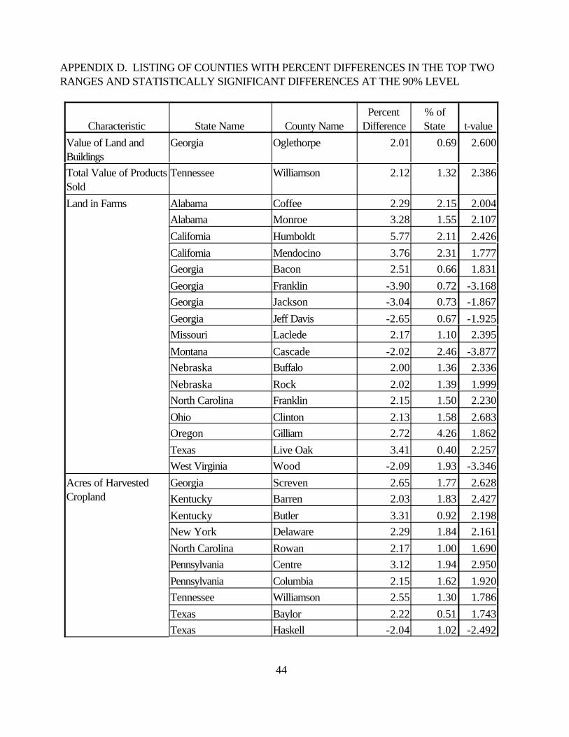
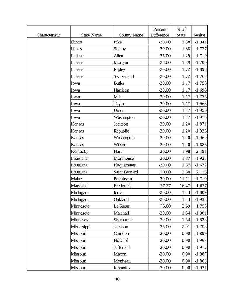
The reader must be careful when using Table 4 tomake comparisons across characteristics, sincethe top two ranges vary by characteristic. Thetop two ranges contain percent differences greaterthan or equal to 2% for the first fivecharacteristics, greater than or equal to 20% forthe last three characteristics, and greater than orequal to 5% for the remaining characteristics. Also, the number of nonsmall counties that werenot significant at the 90% level is included incolumn three of this table. This column plus thenumber of nonsmall counties that were significantat the 90% level (shown in column four) equalsthe total number of nonsmall counties in columntwo. Again, the number of counties at the 95%and 99% significance levels are subsets of theprevious significance level. A listing of all 192

nonsmall county/characteristic combinations thatare statistically significant at the 90% level isprovided in Appendix D. The listing contains thepercent difference and t-value as well as thepercentage of the state total that the countyrepresents.

Table 4 can be compared to Table 2 to evaluatewhether or not the significant differences occurredin the top two ranges for the characteristics. Forexample, Table 2 shows that the percentage ofsignificant counties out of all nonsmall counties forland in farms was 10.18 percent while Table 4shows the percentage of significant counties out ofall nonsmall counties with a percent differencegreater than or equal to 2% was 80.95 percent(17 divided by 21). On the other hand, the same

14

comparison for farms operated by persons ofHispanic origin shows that the percentage ofsignificant counties was 30.95 percent in Table 2and 25.25 percent in Table 4.

A miscellaneous observation for Appendix D isthat Screven, GA had seven characteristics with apercent difference in the top two ranges (the nextclosest county had four). For each characteristic,Screven represented between 1 and 4 percent ofthe state total. All characteristics except for onewere statistically significant at the 95% level.

Again, an interesting subset of the counties talliedin Table 4 is the collection of those counties thatrepresented a substantial percentage of the statetotal. Table 5 provides a listing of the countiesthat had a percent

difference in the top two ranges, and where thecounty represented more than 5 percent of thestate total. Since this subset is only 16 counties,the county names are given with the associatedpercent difference, percentage of state total, andt-value (note that these counties are also listed inAppendix D). If the characteristic does notappear in the table, then there were no countiesthat met these criteria.

Although the same counties appear for acres andbushels of corn for grain harvested, this was notalways the case when examining harvested acresand production for a crop. For example, foracres and bushels of wheat for grain harvested,Appendix D shows that Peach, GA wasstatistically significant for acres but not bushelswhile Morgan, GA was

15

Table 5: Nonsmall Counties with a Percent Difference in the Top Two Ranges that Represent More Than 5 Percent of the State Total

Characteristic State Name County NamePercent

Difference% of State

t-valueAcres of Corn for GrainHarvested

Montana Rosebud 9.89 5.50 2.203Vermont Rutland 5.91 8.51 2.239

Bushels of Corn for GrainHarvested

Montana Rosebud 8.77 5.16 2.243Vermont Rutland 5.03 9.07 2.271

Dollars Received for DairyProducts

Kansas Sedgwick 5.99 5.73 2.138Wyoming Lincoln 5.25 42.20 2.039

Total Hogs and Pigs New Mexico Roosevelt 11.55 6.26 2.514Layers 20 Weeks Old andOlder

Mississippi Leake 6.30 7.76 2.005Mississippi Simpson 6.29 5.23 2.196Nevada Washoe 11.55 12.23 2.071

Broilers and Other Meat-Type Chickens Sold

Colorado Larimer 8.47 10.32 2.162Kansas Reno 9.84 16.46 1.796

Farms Operated by Blacksand Other Races

Massachusetts Barnstable 20.00 11.11 1.921

Farms Operated byPersons of Hispanic Origin

Maine Penobscot 20.00 11.11 1.710Maryland Frederick 27.27 16.47 1.677Wyoming Fremont 21.05 17.56 2.067

statistically significant for bushels but not acres. For the two demographic variables, the percentdifference for Barnstable, MA and Penobscot,ME are a little misleading. These counties werenot small enough to be eliminated from theanalysis, but the weighted number of farms is only4 (not true for the other two counties). Note thatsome of these counties contributed substantially tothe state-level totals being statistically significant. For example, for dollars received for dairyproducts, Lincoln, WY represented 42.20percent of the state total and was statisticallysignificant at the 95% level. Table 1 shows thatWyoming is statistically significant at the 95%level for this characteristic.

An Alternative Weighting Procedure

As previously stated, one of the two main reasonsfor using integer weights is to make the publicationprocess simpler. Record-level integer weightsensure the table cells within a column or row addto the total for the column or row. However,there is another possible way to address thisconcern. Rather than round the nonintegerweights to integer values, another possibleapproach is to apply the noninteger weights to therecord and round the weighted data values at therecord level. Thus, the operation’s weighted datavalues are rounded and these values are used toproduce the totals for the entire population.

To illustrate, recall the previous example wherethe farm had 200 acres of cropland, reported 100acres of soybeans, and 20 cattle. Using the

16

noninteger nonresponse weight of 1.2, the recordrepresented 1.2 farms totaling 240 acres ofcropland, 120 acres of soybeans, and 24 cattle. With the exception of 1.2 farms, no rounding isrequired because the noninteger weight multipliedby the individual data values are already integervalues. This is not a common occurrence inpractice. A more applicable example would bethat the noninteger nonresponse weight for thisrecord is a noninteger value rounded to sixdecimal places, say 1.212684. For this example,the record’s weighted data values are 1.212684farms totaling 242.5368 acres of cropland,121.2684 acres of soybeans, and 24.25368cattle. After the rounding these data values, therecord represents 1 farm totaling 243 acres ofcropland, 121 acres of soybeans, and 24 cattle. For this record, the differences between the totalscalculated with the noninteger weight and therecord’s rounded-weighted data value areminimal.

Totals produced using the record’s rounded-weighted data values are unbiased estimates oftotals produced using the noninteger weights. This procedure performs better than the integerweighting procedure because the two factorsmentioned earlier do not affect this procedure (nothaving a representative sample or the distributionof the data being skewed). However, thedownfall of using this procedure is that it does notwork well when producing totals for indicator orcategorical characteristics. For example, theaverage noninteger nonresponse weight isapproximately 1.139. Therefore, for variablessuch as number of farms and the demographiccharacteristics (Blacks and Other Races,Females, Hispanic Origin), the record’s rounded-weighted data value will round down to one mostof the time and thus underestimate the total.

To examine this methodology on 1997 censusdata, the author selected three states (Georgia,Texas, and Virginia) which showed fairly largedifferences between totals calculated with thenoninteger weights and the published totals. Foreach characteristic, the difference between thetotals calculated with the noninteger and integerweights is compared to the difference between thetotals calculated with the noninteger weights androunded-weighted data values. This analysis wasdone at both the state and county levels. Anoverall summary of these differences is presentedin Appendix E. The table shows the differencesat the state level along with the minimum andmaximum differences at the county level. Asexpected, these results show that the totalsproduced using the rounded-weighted data valuesare more precise than the totals produced usingthe integer weights except for the demographiccharacteristics and number of farms.

RECOMMENDATIONS

The reasons for rounding weights, to ease datareview procedures and to ensure that publicationtotals add, are legitimate concerns. The authorasserts that it is possible to address these twoconcerns and improve the totals produced whenNASS revamps the census processing system forthe 2002 census.

1) Automate the weights into the datareview procedures.

One argument for using the integer weightsis that one can “easily” obtain weightedtotals for a record of interest during thedata review phase. In the 1997 system,this would be accomplished by multiplyingthe integer weight by each record’s datavalue of interest. Thus, this manualcomputation is easier if the nonresponse

17

weight is 2 rather than 1.7. However, for the2002 system, the computer can and shouldperform this calculation. With thisimprovement, the value of the weight is nolonger relevant.

2) Use a combination of the integer weightsand the record’s rounded-weighted datavalues.

Another argument for using the integer weightsis to ensure that publication totals add. Integerweights should be used to produce totals forindicator and categorical variables. Thesevariables include number of farms as well asvariables for the questions concerning type oforganization, corporate structure, andcharacteristics and occupation of the operator(which includes demographic characteristics). In addition, the integer weights should be usedfor any question where the data values aresmall for most farms. For the 1997 census,the only example of this is the questionconcerning injuries or deaths. The record’srounded-weighted data values should be usedto produce totals for all other characteristics. Here, the noninteger weight is applied to therecord and the weighted data values arerounded at the record level. With thisimprovement, the integer sample item weightshould no longer be necessary since the 1997long form did not contain a question thatrequires it.

3) Evaluate the 2002 questionnaires todetermine which weight to use.

Once the 2002 long and short forms arefinalized, the questions will need to beevaluated to determine which weight to useduring the summarization process. Inparticular, the questions on the 2002 long formwill determine whether the integer sample itemweight is needed.

18

REFERENCES

Swan, Carolyn, “1997 Nonresponse Weighting:Nonresponse Survey Sampling Specification,”NASS Internal Memo, April 1999.

Scholetzky, Wendy, “1997 NonresponseWeighting: Creation of Final NonresponseWeighting Short Record File,” NASS InternalMemo, April 1999.

Swan, Carolyn, “Estimation of In-ScopeNonrespondents and Calculation of InitialNoninteger Nonresponse Weights atCounty/Nonresponse Stratum Level,” NASSInternal Memo, April 1999.

Scholetzky, Wendy, “1997 NonresponseWeighting: Final Nonresponse WeightingSpecification,” NASS Internal Memo, April1999.

Scholetzky, Wendy, “1997 Census of Agriculture- Sample Weighting Specifications,” NASSInternal Memo, April 1999.

Kraus, Melinda and Winters, Franklin, “AnEvaluation of Rounding Techniques Used toObtain Estimated Totals,” American StatisticalAssociation, 1993 Proceedings of theInternational Conference on EstablishmentSurveys, pp. 893-898.

19

APPENDIX A. FORMULA FOR CALCULATING THE STANDARD ERROR OF THEDIFFERENCE

The following formula was used for calculating the standard error of the difference between the totalsgenerated using integer and noninteger weights:

Standard Error of Difference ' jJ

j'1jH

h'1

nhj

nhj & 1 jn hj

i'1[wihj(yihj & yh(w)) & aihj(yihj & yh(a))]

2

where

nhj = the number of in-scope, interviewed records in stratum h in county j

wihj = the noninteger weight associated with record i in stratum h in county j

aihj = the integer weight associated with record i in stratum h in county j

yihj = the unweighted data value for record i in stratum h in county j

= the weighted average total for stratum h in county j using the noninteger weightsyh(w)

= the weighted average total for stratum h in county j using the integer weightsyh(a)

H = the number of nonresponse strata in the county for characteristics on both the long and short forms

or= the number of sample strata in the county for long-form characteristics

J = the number of counties in the state for state-level totals or

= 1 for county-level totals

20

21

APPENDIX B. LISTING OF STATES WITH STATISTICALLY SIGNIFICANT DIFFERENCESAT THE 90% LEVEL

Characteristic State NamePercent

Difference Difference t-valueValue of Land andBuildings

Colorado 0.27 53,982,465 1.789Kentucky -0.09 -17,501,972 -1.960Louisiana 0.21 19,204,512 1.790Maryland 0.25 16,990,601 2.036Michigan 0.14 22,722,570 2.024Montana -0.15 -25,874,963 -1.712North Carolina -0.14 -26,145,535 -2.259Oklahoma -0.18 -35,755,465 -2.675South Carolina -0.22 -14,636,941 -1.907Vermont -0.36 -6,858,242 -1.869

Farm ProductionExpenditures

North Dakota -0.05 -1,187,380 -1.732

Total Value ofProducts Sold

Arizona -0.11 -2,180,052 -3.358

Land in Farms California 0.40 111,717 2.287Georgia -0.25 -26,798 -2.327Oklahoma 0.12 41,009 1.673

Acres of HarvestedCropland

Arizona -0.26 -2,492 -2.440Arkansas 0.13 10,164 1.941Connecticut -0.56 -793 -1.687Hawaii -0.21 -213 -2.091Maine -0.45 -1,804 -1.745North Carolina -0.18 -7,833 -1.964South Dakota -0.15 -21,711 -2.002

Acres of Corn forGrain Harvested

Colorado -0.37 -3,397 -1.814Delaware 0.63 989 1.708Kansas -0.20 -4,976 -1.646Louisiana -0.42 -1,725 -1.898New Hampshire -1.46 -18 -1.800North Dakota -0.35 -2,044 -1.659Vermont -1.75 -147 -2.940


Difference Difference t-value

22

Bushels of Corn forGrain Harvested

Delaware 0.81 126,614 2.208Kansas -0.21 -748,562 -1.807New Hampshire -1.26 -1,622 -1.816North Dakota -0.37 -203,715 -1.747Vermont -1.58 -15,061 -2.791Wyoming -1.58 -100,573 -1.979

Acres of Wheat forGrain Harvested

Iowa -2.36 -535 -1.701Mississippi -0.58 -901 -1.818Nevada -1.28 -247 -2.150New York -0.93 -1,137 -3.118

Bushels of Wheat forGrain Harvested

Florida -2.35 -14,088 -1.716Iowa -2.61 -24,231 -1.766Mississippi -0.49 -31,983 -1.713Nevada -1.11 -21,468 -2.816New York -0.72 -46,268 -2.710

Acres of SoybeansHarvested

Alabama 0.81 2,537 1.731Oklahoma -0.81 -2,654 -1.879

Acres of CottonHarvested

Missouri -0.37 -1,457 -1.661

Bales of CottonHarvested

Missouri -0.43 -2,401 -2.125New Mexico -0.66 -754 -1.895

Total Cattle andCalves

Kentucky -0.23 -5,500 -1.736Vermont 0.48 1,483 2.292Wisconsin -0.19 -6,492 -1.793

Dollars Received forDairy Products

Delaware 1.32 250,408 1.666Illinois 1.33 3,329,056 2.359Louisiana 1.21 1,243,682 2.655Mississippi -0.97 -816,420 -2.549Utah 0.25 496,490 1.675Wyoming -2.59 -262,555 -2.140

Total Hogs and Pigs Louisiana -2.11 -439 -2.905New Mexico -5.08 -327 -2.399Ohio -0.43 -7,418 -1.773Tennessee -1.21 -3,933 -4.743


Difference Difference t-value

23

Layers 20 Weeks Oldand Older

Maryland 0.81 33,018 1.645New Hampshire -0.39 -721 -2.077Pennsylvania 0.24 57,715 2.064Vermont 0.34 864 1.965Wisconsin -0.32 -12,011 -1.804

Broilers and OtherMeat-Type ChickensSold

Kansas -9.10 -3,507 -2.627Maine -0.40 -807 -1.699Wisconsin -0.13 -36,844 -2.098

Farms Operated byBlacks and OtherRaces

Arizona -2.63 -14 -2.490Kentucky 2.92 20 2.168New Mexico 0.99 21 1.681

Farms Operated byFemales

Colorado 1.04 33 2.034Georgia -0.75 -32 -1.726Hawaii 2.33 21 2.167Maine 1.99 16 1.911Minnesota -1.09 -40 -2.173North Dakota 2.85 37 2.875South Dakota -1.60 -24 -2.360

Farms Operated byPersons of HispanicOrigin

Indiana -2.93 -7 -1.853Kentucky 3.58 14 2.054Maryland 8.97 7 2.195Michigan -3.78 -11 -3.036Minnesota 4.84 12 2.166New Mexico -0.69 -24 -1.730Ohio -3.77 -12 -2.750Oregon -2.48 -13 -2.190Wisconsin -3.46 -9 -2.054Wyoming 6.50 8 2.122

24

APPENDIX C. COUNTY-LEVEL MAPS OF PERCENT DIFFERENCES

44

APPENDIX D. LISTING OF COUNTIES WITH PERCENT DIFFERENCES IN THE TOP TWORANGES AND STATISTICALLY SIGNIFICANT DIFFERENCES AT THE 90% LEVEL


Difference% ofState t-value

Value of Land andBuildings

Georgia Oglethorpe 2.01 0.69 2.600

Total Value of ProductsSold

Tennessee Williamson 2.12 1.32 2.386

Land in Farms Alabama Coffee 2.29 2.15 2.004Alabama Monroe 3.28 1.55 2.107California Humboldt 5.77 2.11 2.426California Mendocino 3.76 2.31 1.777Georgia Bacon 2.51 0.66 1.831Georgia Franklin -3.90 0.72 -3.168Georgia Jackson -3.04 0.73 -1.867Georgia Jeff Davis -2.65 0.67 -1.925Missouri Laclede 2.17 1.10 2.395Montana Cascade -2.02 2.46 -3.877Nebraska Buffalo 2.00 1.36 2.336Nebraska Rock 2.02 1.39 1.999North Carolina Franklin 2.15 1.50 2.230Ohio Clinton 2.13 1.58 2.683Oregon Gilliam 2.72 4.26 1.862Texas Live Oak 3.41 0.40 2.257West Virginia Wood -2.09 1.93 -3.346

Acres of HarvestedCropland

Georgia Screven 2.65 1.77 2.628Kentucky Barren 2.03 1.83 2.427Kentucky Butler 3.31 0.92 2.198New York Delaware 2.29 1.84 2.161North Carolina Rowan 2.17 1.00 1.690Pennsylvania Centre 3.12 1.94 2.950Pennsylvania Columbia 2.15 1.62 1.920Tennessee Williamson 2.55 1.30 1.786Texas Baylor 2.22 0.51 1.743Texas Haskell -2.04 1.02 -2.492



45

West Virginia Wood -2.41 2.02 -2.498Acres of Corn forGrain Harvested

Alabama Marion 8.52 1.66 1.914Florida Walton 8.57 2.06 1.705Georgia Jeff Davis -5.87 0.97 -1.668Georgia Screven 6.37 2.56 2.947Montana Rosebud -9.89 5.50 -2.203Texas Bexar -5.33 0.66 -2.226Texas Cameron 5.93 0.85 1.976Vermont Rutland -5.91 8.51 -2.239Virginia Lancaster 6.36 1.31 1.727Virginia Page 5.90 1.07 1.835

Bushels of Corn forGrain Harvested

Georgia Screven 5.92 2.31 2.673Montana Rosebud -8.77 5.16 -2.243Texas Cameron 6.51 0.74 2.071Vermont Rutland -5.03 9.07 -2.271

Acres of Wheat forGrain Harvested

Florida Santa Rosa -5.40 3.99 -2.076Georgia Peach -7.01 0.93 -1.717Georgia Screven 6.08 1.12 2.038Georgia Taylor -5.14 0.65 -1.727Indiana Randolph 6.61 1.73 2.991Iowa Benton -10.91 1.11 -1.683Iowa Linn -14.35 1.86 -1.741Iowa Page -10.14 1.76 -2.371Virginia Middlesex 6.30 1.60 2.157

Bushels of Wheat forGrain Harvested

Georgia Morgan -5.76 0.74 -1.901Georgia Screven 5.24 1.21 2.115Indiana Randolph 6.77 1.81 2.970Iowa Benton -11.00 1.05 -1.682Iowa Page -9.62 1.52 -2.414

Acres of SoybeansHarvested

Georgia Screven 5.15 4.11 2.311Georgia Telfair -12.72 0.66 -1.807Pennsylvania Snyder 5.15 1.72 1.676Texas Red River 10.27 4.56 1.725Virginia Middlesex 6.53 1.69 2.625



46

Bushels of SoybeansHarvested

Florida Holmes -6.98 2.72 -1.694Georgia Telfair -20.75 0.65 -1.732Pennsylvania Snyder 6.44 1.88 1.821Virginia Middlesex 7.29 1.34 3.267

Total Cattle and Calves Georgia Thomas -5.94 0.73 -2.916Dollars Received forDairy Products

Illinois Douglas 16.99 1.09 1.734Illinois Ogle 10.64 1.95 1.707Kansas Sedgwick 5.99 5.73 2.138Kentucky Edmonson 9.20 0.88 1.683Mississippi Marion 8.57 4.55 1.659Mississippi Pearl River -5.47 1.39 -1.972Nebraska Boone -6.05 1.39 -1.706Nebraska Saunders -10.25 1.17 -2.086South Dakota Bon Homme -6.42 1.85 -3.146South Dakota Gregory 9.19 2.80 1.788Tennessee Williamson 6.86 1.84 2.005West Virginia Ohio -9.18 3.17 -2.364Wyoming Lincoln -5.25 42.20 -2.039

Total Hogs and Pigs Alabama Madison -6.67 1.73 -1.765Florida Hernando -12.15 1.74 -1.703Idaho Gem -5.29 2.35 -1.793Louisiana Calcasieu -7.86 2.88 -2.654New Mexico Roosevelt -11.55 6.26 -2.514Texas Fayette -5.00 1.07 -2.102Wisconsin Outagamie -5.34 1.79 -3.478

Layers 20 Weeks Oldand Older

Alabama Cleburne -6.78 1.60 -1.970Arkansas Yell -7.18 2.63 -1.767Mississippi Jefferson Davis -17.64 2.56 -2.003Mississippi Leake -6.30 7.76 -2.005Mississippi Simpson -6.29 5.23 -2.196Missouri Pettis -8.06 1.88 -1.829Nevada Washoe -11.55 12.23 -2.071



47

Broilers and OtherMeat-Type ChickensSold

Colorado Larimer -8.47 10.32 -2.162

Kansas Reno -9.84 16.46 -1.796

Farms Operated byBlacks and OtherRaces

Arkansas Clark 25.00 2.14 1.975Georgia Baldwin 28.57 0.68 1.734Georgia Monroe 37.50 0.83 1.965Indiana Allen -25.00 1.74 -1.725Indiana Lake -25.00 1.74 -1.645Indiana Putnam -20.00 2.33 -1.927Iowa Lee -20.00 3.25 -1.727Massachusetts Barnstable -20.00 11.11 -1.921Minnesota Clearwater -20.00 2.04 -1.863Minnesota Morrison -20.00 2.04 -1.944Minnesota Otter Tail 40.00 3.57 1.663Nebraska Douglas -25.00 1.59 -1.649Nebraska Sioux -25.00 1.59 -1.741Nebraska Thurston -20.00 4.23 -2.105Ohio Ashtabula 37.50 3.45 1.806Wisconsin Pierce -20.00 2.17 -1.956Wisconsin Washburn -25.00 1.63 -1.646

Farms Operated byFemales

North Dakota Pierce 20.83 2.17 2.105

Farms Operated byPersons of HispanicOrigin

Alabama Jackson -25.00 1.61 -1.683Alabama Shelby -20.00 2.15 -1.653Alabama Washington -20.00 2.15 -1.946Georgia Cobb -25.00 0.96 -1.971Georgia Turner -25.00 0.96 -1.717Illinois Bureau -20.00 1.38 -1.961Illinois Calhoun -25.00 1.04 -1.870Illinois Champaign -20.00 1.38 -1.976Illinois Effingham -20.00 1.38 -1.726Illinois Fayette -25.00 1.04 -1.726Illinois Macoupin -20.00 1.38 -1.666Illinois Peoria -20.00 1.38 -1.984



48

Illinois Pike -20.00 1.38 -1.941Illinois Shelby -20.00 1.38 -1.777Indiana Allen -25.00 1.29 -1.719Indiana Morgan -25.00 1.29 -1.700Indiana Ripley -20.00 1.72 -1.895Indiana Switzerland -20.00 1.72 -1.764Iowa Butler -20.00 1.17 -1.753Iowa Harrison -20.00 1.17 -1.698Iowa Mills -20.00 1.17 -1.776Iowa Taylor -20.00 1.17 -1.968Iowa Union -20.00 1.17 -1.956Iowa Washington -20.00 1.17 -1.970Kansas Jackson -20.00 1.20 -1.871Kansas Republic -20.00 1.20 -1.926Kansas Washington -20.00 1.20 -1.969Kansas Wilson -20.00 1.20 -1.686Kentucky Hart -20.00 1.98 -2.491Louisiana Morehouse -20.00 1.87 -1.937Louisiana Plaquemines -20.00 1.87 -1.672Louisiana Saint Bernard 20.00 2.80 2.115Maine Penobscot -20.00 11.11 -1.710Maryland Frederick 27.27 16.47 1.677Michigan Ionia -20.00 1.43 -1.809Michigan Oakland -20.00 1.43 -1.933Minnesota Le Sueur 75.00 2.69 1.755Minnesota Marshall -20.00 1.54 -1.901Minnesota Sherburne -20.00 1.54 -1.838Mississippi Jackson -25.00 2.01 -1.753Missouri Camden -20.00 0.90 -1.899Missouri Howard -20.00 0.90 -1.963Missouri Jefferson -20.00 0.90 -1.912Missouri Macon -20.00 0.90 -1.987Missouri Moniteau -20.00 0.90 -1.863Missouri Reynolds -20.00 0.90 -1.921



49

Missouri Warren -20.00 0.90 -1.845Montana Missoula -20.00 2.31 -1.948Nebraska Butler -25.00 1.18 -1.724Nebraska Cheyenne -20.00 1.57 -1.857Nebraska Nuckolls -25.00 1.18 -1.733Nebraska Otoe -25.00 1.18 -1.736Nebraska Seward -25.00 1.18 -1.709Nebraska Sioux -20.00 1.57 -1.945North Carolina Alexander -20.00 1.25 -1.647North Carolina Davidson -20.00 1.25 -1.729North Carolina Iredell -22.22 2.19 -2.127North Carolina Pender -20.00 1.25 -1.697North Dakota Oliver -25.00 2.07 -1.733North Dakota Pembina -20.00 2.76 -1.699North Dakota Williams -20.00 2.76 -1.731Ohio Clermont -20.00 1.31 -1.948Ohio Gallia -20.00 1.31 -1.704Ohio Geauga -20.00 1.31 -1.917Ohio Madison -20.00 1.31 -1.940Oklahoma Payne 23.08 2.90 1.825South Dakota Day 60.00 4.76 1.693South Dakota Turner -20.00 2.38 -1.931Tennessee Cannon -20.00 1.07 -1.688Tennessee Davidson -28.57 1.33 -2.209Tennessee Dickson -20.00 1.07 -1.915Tennessee Mcnairy -20.00 1.07 -1.957Virginia Frederick -20.00 1.72 -1.964Wisconsin Clark -20.00 1.59 -1.931Wisconsin Eau Claire -20.00 1.59 -1.923Wisconsin Shawano -20.00 1.59 -1.986Wyoming Fremont 21.05 17.56 2.067

50

APPENDIX E. SUMMARY OF DIFFERENCES BETWEEN STATE AND COUNTY TOTALSFOR GEORGIA, TEXAS, AND VIRGINIA

Georgia data - 1997 census

Characteristic LevelInteger Total -

Noninteger TotalRounded Total -Noninteger Total

Value of Land and state -7,033,641 72Buildings min cnty -2,892,379 -5

max cnty 2,881,849 5Farm Production state -207,412 60Expenditures min cnty -135,120 -8

max cnty 204,418 6Total Value of Products state -1,410,654 180Sold min cnty -536,106 -9

max cnty 463,555 11Land in Farms state -26,801 303

min cnty -3,529 -13max cnty 2,403 18

Acres of Harvested state -4,889 32Cropland min cnty -1,393 -13

max cnty 1,723 9Acres of Corn for state -885 35Grain Harvested min cnty -348 -5

max cnty 620 4Bushels of Corn for state -130,369 27Grain Harvested min cnty -34,972 -4

max cnty 52,426 6Acres of Wheat for state -1,777 5Grain Harvested min cnty -354 -4

max cnty 404 3Bushels of Wheat for state -56,259 6Grain Harvested min cnty -18,331 -3

max cnty 19,843 3Acres of Soybeans state -296 15Harvested min cnty -340 -2

max cnty 706 3Bushels of Soybeans state 1,065 27Harvested min cnty -12,088 -2

max cnty 15,117 5Acres of Cotton state -1,202 9Harvested min cnty -723 -3

max cnty 697 3

Georgia data - 1997 census



51

Bales of Cotton state -943 18Harvested min cnty -995 -4

max cnty 900 5Total Cattle and Calves state -3,759 182

min cnty -630 -15max cnty 659 9

Dollars Received for state 93,501 -3Dairy Products min cnty -120,013 -1

max cnty 140,939 1Total Hogs and Pigs state 2,858 -1


Layers 20 Weeks Old state -79,527 4and Older min cnty -31,671 -4

max cnty 19,248 4Broilers and Other state -445,904 1Meat-Type Chickens min cnty -935,341 -1Sold max cnty 450,302 1Farms Operated by state 7 -151Blacks and Other min cnty -3 -8Races max cnty 3 1Farms Operated by state -33 -443Females min cnty -5 -10

max cnty 4 1Farms Operated by state 6 -25Persons of Hispanic min cnty -1 -1Origin max cnty 1 0Number of Farms state 0 -4,014

min cnty 0 -92max cnty 0 6

Texas data - 1997 census



Value of Land and state 3,016,549 316Buildings min cnty -6,887,964 -6

max cnty 5,526,046 15Farm Production state 1,048,512 -1Expenditures min cnty -222,899 -10

max cnty 214,559 12




52

Total Value of Products state -92,594 558Sold min cnty -501,672 -21

max cnty 990,152 37Land in Farms state -45,143 285

min cnty -10,832 -45max cnty 20,212 54

Acres of Harvested state -3,658 181Cropland min cnty -4,155 -64

max cnty 2,402 60Acres of Corn for state -451 2Grain Harvested min cnty -766 -6

max cnty 979 6Bushels of Corn for state -44,145 -12Grain Harvested min cnty -145,745 -3

max cnty 99,626 3Acres of Wheat for state -748 14Grain Harvested min cnty -2,314 -6

max cnty 2,359 8Bushels of Wheat for state -1,629 44Grain Harvested min cnty -36,454 -6

max cnty 67,443 12Acres of Soybeans state 2,107 7Harvested min cnty -384 -2

max cnty 1,618 3Bushels of Soybeans state 9,886 5Harvested min cnty -11,092 -4

max cnty 24,216 2Acres of Cotton state 2,827 25Harvested min cnty -1,488 -4

max cnty 1,970 7Bales of Cotton state 2,705 -5Harvested min cnty -1,103 -4

max cnty 2,047 6Total Cattle and Calves state 1,986 701

min cnty -1,834 -41max cnty 1,621 45

Dollars Received for state 325,215 9Dairy Products min cnty -274,514 -2

max cnty 354,517 2




53

Total Hogs and Pigs state -1,281 -147min cnty -357 -7max cnty 744 6


max cnty 31,572 8Broilers and Other state -324,496 -1Meat-Type Chickens min cnty -170,131 -1Sold max cnty 118,908 1Farms Operated by state 3 -1,223Blacks and Other min cnty -5 -47Races max cnty 9 1Farms Operated by state -51 -3,053Females min cnty -14 -53

max cnty 11 1Farms Operated by state 3 -1,164Persons of Hispanic min cnty -8 -95Origin max cnty 10 1Number of Farms state 0 -26,925


Virginia data - 1997 census



Value of Land and state 720,977 128Buildings min cnty -2,328,309 -5

max cnty 3,887,524 15Farm Production state -76,832 34Expenditures min cnty -116,301 -6

max cnty 196,232 6Total Value of Products state -575,119 170Sold min cnty -346,315 -33

max cnty 414,753 14Land in Farms state 6,261 119

min cnty -2,538 -21max cnty 1,933 21

Acres of Harvested state 604 -206Cropland min cnty -582 -53

max cnty 893 15




54

Acres of Corn for state 717 -27Grain Harvested min cnty -171 -9

max cnty 283 5Bushels of Corn for state 81,713 19Grain Harvested min cnty -19,575 -4

max cnty 26,827 6Acres of Wheat for state 302 7Grain Harvested min cnty -175 -6

max cnty 259 7Bushels of Wheat for state 2,761 11Grain Harvested min cnty -13,882 -7

max cnty 19,456 4Acres of Soybeans state 1,537 27Harvested min cnty -338 -2

max cnty 617 4Bushels of Soybeans state 22,121 3Harvested min cnty -9,354 -3

max cnty 13,408 4Acres of Cotton state 95 6Harvested min cnty -86 0

max cnty 104 2Bales of Cotton state 103 3Harvested min cnty -112 -1

max cnty 104 2Total Cattle and Calves state 1,085 -22


Dollars Received for state -292,542 2Dairy Products min cnty -122,914 -3

max cnty 102,213 2Total Hogs and Pigs state 972 -56



max cnty 14,642 3Broilers and Other state -493,666 1Meat-Type Chickens min cnty -423,092 -1Sold max cnty 65,829 1




55

Farms Operated by state 11 -143Blacks and Other min cnty -5 -19Races max cnty 3 0Farms Operated by state -7 -473Females min cnty -5 -25

max cnty 9 0Farms Operated by state 7 -12Persons of Hispanic min cnty -1 -1Origin max cnty 2 0Number of Farms state 0 -4,110


Documents

EVALUATION OF INTEGER WEIGHTING FOR THE … OF INTEGER WEIGHTING FOR THE 1997 CENSUS OF AGRICULTURE, ... Wade for the Mapinfo tutorial, and Phil Kott for …