Evaluation of frescoes detachments by partial least square

Evaluation of frescoes detachments by partial least square thermography

by P. Bison*, A. Bortolin*, G. Cadelano*, G. Ferrarini*, L. Finesso**, F. Lopez***, X. Maldague**** *ITC-CNR, Corso Stati Uniti 4, 35127 Padova Italy, [email protected] **ISIB-CNR, Corso Stati Uniti 4, 35127 Padova Italy. ***Dept. of Mechanical Engineering, Federal University of Santa Catarina, 88040-900,Florianópolis, Santa Catarina. ****Electrical and Computing Engineering Dept., Laval University, Quebec City (Quebec), Canada G1K 7P4.

Abstract

Several image processing algorithms are available to enhance the results of non destructive evaluation of artworks. This work is focused on the novel Partial Least Squares Thermography (PSLT) technique, that allows a strong data compression. A preliminary test on a fresco sample and a wide survey of the San Gottardo Church (located in Asolo, Italy) have been conducted to locate detachments with an active thermography technique. All the obtained thermal sequences have been post processed with different algorithms, including Principal Component Thermography (PCT), Thermographic Signal Reconstruction (TSR) and PLST. For the latter, two different approaches have been proposed and compared.

1. Introduction

Infrared thermography is a powerful technique that is commonly utilized for non destructive evaluation of materials and specimens [1]. Because infrared thermography allows contactless and non-invasive surveys of artworks, both in laboratory and on site, various types of applications have been proposed in the cultural heritage field [2-6]. Among the main objectives of the thermographic inspections there are the hidden structure detection and the evaluation of damages related to moisture, delamination or ageing. The on-site evaluation must deal with practical challenges, such as the difficulty to reach the observed objects or the availability of the site that can be limited.

The object of this paper is the survey of San Gottardo Church, located in Asolo (North-East of Italy), that dates back to the XIII century. Inside this building several frescoes are showing both visible and hidden detachments. Literature proposes various active thermographic techniques [7,8] for the analysis of frescoes specimens that can be applied both in the laboratory and on-site. After the acquisition of multiple infrared images, processing algorithms [9] could be applied to the data: in this work the partial least square thermography [10] analysis has been applied and compared to other standard algorithms.

2. Thermal model

Fresco is a painting technique that has been frequently applied inside Italian historical buildings such as churches to decorate the walls. The creation of a frescoed surface starts when the inner surface of a wall, that is usually made of stones or bricks, is coated with “arriccio”. This is a compound of lime plaster and coarse sand that is placed in order to make a flat surface. Then another layer, called “intonaco”, is applied on the surface. This latter layer is made of lime plaster and fine sand and it contains the pigments. Occasionally more than one layer of “intonaco” could be present, as a new fresco could be superimposed to the previous one.

Even if a fresco could last for hundreds of year, frequently older artworks show unambiguous clear signs of deterioration. This is due to several causes, including biological patina or mechanical damages caused by water. Besides these, the most widespread causes of deterioration are efflorescence and subflorescence of new formed minerals. The latter in particular occurs under the surface, and makes themselves into internal voids or cracks, that are invisible to the observer but can seriously damage the fresco causing detachments.

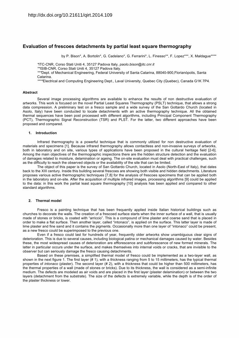
Based on these premises, a simplified thermal model of fresco could be implemented as a two-layer wall, as shown in the next figure 1. The first layer (# 1), with a thickness ranging from 5 to 15 millimeters, has the typical thermal properties of intonaco (plaster). The second layer (# 2), with a thickness that could be higher than 500 millimeters, has the thermal properties of a wall (made of stones or bricks). Due to its thickness, the wall is considered as a semi-infinite medium. The defects are modeled as air voids and are placed in the first layer (plaster delamination) or between the two layers (detachment from the substrate). The size of the defects is extremely variable, while the depth is of the order of the plaster thickness or lower.

http://dx.doi.org/10.21611/qirt.2014.109

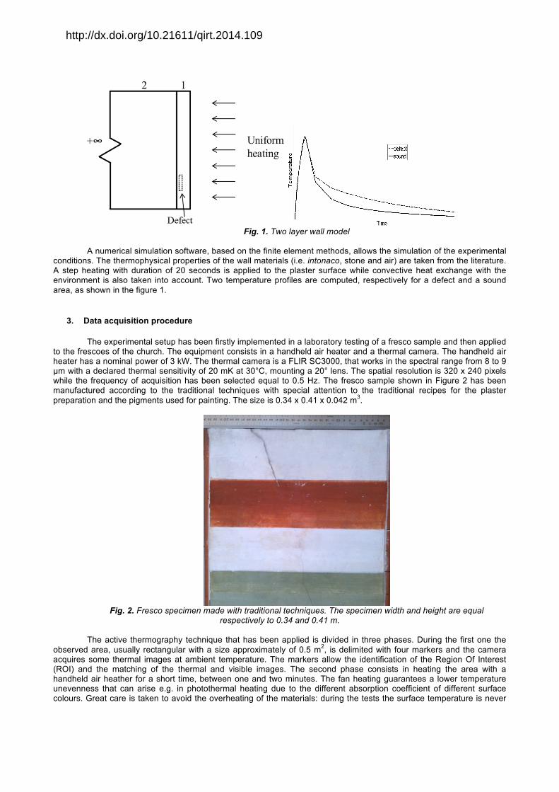
Fig. 1. Two layer wall model

A numerical simulation software, based on the finite element methods, allows the simulation of the experimental

conditions. The thermophysical properties of the wall materials (i.e. intonaco, stone and air) are taken from the literature. A step heating with duration of 20 seconds is applied to the plaster surface while convective heat exchange with the environment is also taken into account. Two temperature profiles are computed, respectively for a defect and a sound area, as shown in the figure 1.

3. Data acquisition procedure

The experimental setup has been firstly implemented in a laboratory testing of a fresco sample and then applied to the frescoes of the church. The equipment consists in a handheld air heater and a thermal camera. The handheld air heater has a nominal power of 3 kW. The thermal camera is a FLIR SC3000, that works in the spectral range from 8 to 9 µm with a declared thermal sensitivity of 20 mK at 30°C, mounting a 20° lens. The spatial resolution is 320 x 240 pixels while the frequency of acquisition has been selected equal to 0.5 Hz. The fresco sample shown in Figure 2 has been manufactured according to the traditional techniques with special attention to the traditional recipes for the plaster preparation and the pigments used for painting. The size is 0.34 x 0.41 x 0.042 m3.

Fig. 2. Fresco specimen made with traditional techniques. The specimen width and height are equal

respectively to 0.34 and 0.41 m.

The active thermography technique that has been applied is divided in three phases. During the first one the observed area, usually rectangular with a size approximately of 0.5 m2, is delimited with four markers and the camera acquires some thermal images at ambient temperature. The markers allow the identification of the Region Of Interest (ROI) and the matching of the thermal and visible images. The second phase consists in heating the area with a handheld air heather for a short time, between one and two minutes. The fan heating guarantees a lower temperature unevenness that can arise e.g. in photothermal heating due to the different absorption coefficient of different surface colours. Great care is taken to avoid the overheating of the materials: during the tests the surface temperature is never


increased more than 5 degrees above the initial temperature. The last part is the recording of thermal images at 0.5 Hz frequency for few minutes after removing the heater, until the surface temperature variation over time is negligible.

4. Image processing

The sequence of IR images taken during the experiment can be arranged in a three dimensional matrix, having height and width equal to the size of the observed area and depth equal to the number of acquired images. The image processing algorithms that have been applied to the thermal sequences are Principal Component Thermography (PCT), Temperature Signal Reconstruction (TSR) and Partial Least Squares Thermography, that has been proposed with two approaches. The first one, more similar to PCT, is named PLST; the second one, more similar to TSR, is named PLSRT.

4.1 Principal Component Thermography (PCT)

A commonly used image processing technique is Principal Component Thermography (PCT) [11-13], that relies on the statistical procedure named Principal component analysis (PCA). This technique applies orthogonal transformations to a set of observations of possibly correlated variables in order to transform it into a set of linearly uncorrelated variables. These values are the principal components; their number is equal or lower than the number of original variables. Principal component thermography execute on the data a singular value decomposition (SVD), a procedure that allows to obtain spatial and temporal data from a matrix in a simplified way. SVD provides at the same time the PCAs for both the row and column spaces. Considering a matrix X ∈ Rpxq, with p<q, its singular value decomposition is obtained as:

TUSVX= (1) where U is an p x q matrix with orthogonal columns, S is a diagonal matrix (q x q) with the singular values of X

on the diagonal, and VT is a (q x q) orthogonal matrix. The original thermal sequence T is three dimensional (a,b,n), therefore it must be reshaped into a two dimensional matrix Tr ∈ Rpxq having a x b≡q columns and n≡p rows. In this manner the temperature profiles of each pixel are arranged vertically. After the application of the SVD to the Tr matrix, the U matrix is composed by a set of empirical orthogonal functions (EOF) that describe the temporal variations of data, while the rows of the VT matrix are the principal components, that describe spatial variations. The data are represented by the EOF ordered in a decreasing way: the first one contains the most part of variation, the following less and less. In this way the information contained in a thermal sequence can be compressed in few images, typically less than ten.

4.2 Thermographic Signal Reconstruction (TSR)

Thermographic Signal Reconstruction (TSR) [14-16] is widely applied in Non-Destructive Testing and Evaluation. This method is based on the solution of the one dimensional heat conduction equation on a semi-infinite body that has been subject to a pulsed thermal excitation. This procedure analyzes the data acquired with pulsed thermographic experiments, fitting the experimental data represented in log-log space polynomial function as:

n

n2

210 )]t[ln(a...)]t[ln(a)tln(aa)Tln( ++++=Δ (2) where ΔT is the temperature profile of a single pixel during the experiment and a0, a1,…, an are the coefficients

of the polynomial fitting. The fitting is calculated for every pixel of the thermal image, obtaining the corresponding maps of coefficients. As in PCT, it is therefore possible to compress the original three dimensional data matrix T into a smaller one that maintains the same width and height but changes its depth, that is equal to n, the degree of the polynomial fitting. The latter value is variable, in this works it has been set to 5.

4.3 Partial Least Squares Thermography (PLST) and Partial Least Squares Regression Thermography (PLSRT)

The Partial Least Squares (PLS) [17] is a family of statistical procedures that is commonly applied in different fields, such as chemistry, economics and neuroscience. PLS methods include correlation, regression and path modelling techniques. One of the advantages of these techniques is the possibility of analyzing simultaneously two matrices X and Y, taking into account the relationship between each other. One of these matrices is necessarily the data matrix, the second one could be the time vector or a model matrix. After choosing a number of components c (usually similar to the useful components of PCA) PLS performs the simultaneous decomposition of both X and Y. Mathematically, PLS is expressed as follows:


EPTX T +⋅= (3)

FQTY T +⋅= (4) where P and Q are defined as loadings, T is an orthonormal matrix defined as score and E and F are residuals.

If X ∈ Rnxs and Y ∈ Rnxm, then the loading P ∈ Rsxc, the loading Q ∈ Rmxc and the score T ∈ Rnxc. Different algorithms are available to calculate the PLS, in this work the SIMPLS algorithm has been applied [18]. The data matrix could be the X or the Y matrix, leading in the first case to the PLST approach [10] and in the second case to the PLSRT approach. With the former, the X matrix is the data matrix while the Y is a time vector with all the ordered acquisition time of the experiment or their corresponding frequencies. With the latter PLSRT approach, the Y matrix is the data matrix and the X matrix is a model matrix that can be connected by the following linear equation:

EBXY +⋅= (5)

where B is a coefficient matrix that with the utilized implementation of the SIMPLS algorithm has s+1 rows and m columns. The choice of the model matrix X is related to the type of experiment; in this work a similarity with TSR has been investigated. For this reason the regression is executed in logarithmic scales, as in:

EB)t(log)t(log

)t(log)t(log

)tlog(

)tlog(

1

1

)Tlog()Tlog(

)Tlog()Tlog(

n4

n2

14

12

n

1

n,pn,1

1,p1,1+⋅

⎥⎥⎥⎥

⎦

⎤

⎢⎢⎢⎢

⎣

⎡

=⎥⎥⎥

⎦

⎤

⎢⎢⎢

⎣

⎡

(6)

In this work the number of components c has been set to 5.

5. Results – Laboratory testing

Receiver operating characteristic (ROC) analysis arises from the theory of signal detection, as a model of how well the receiver can detect a signal in presence of noise. Its main feature is the discrimination between the hit rate (or true positive rate) and the rate of false positives as two separate performances [19].

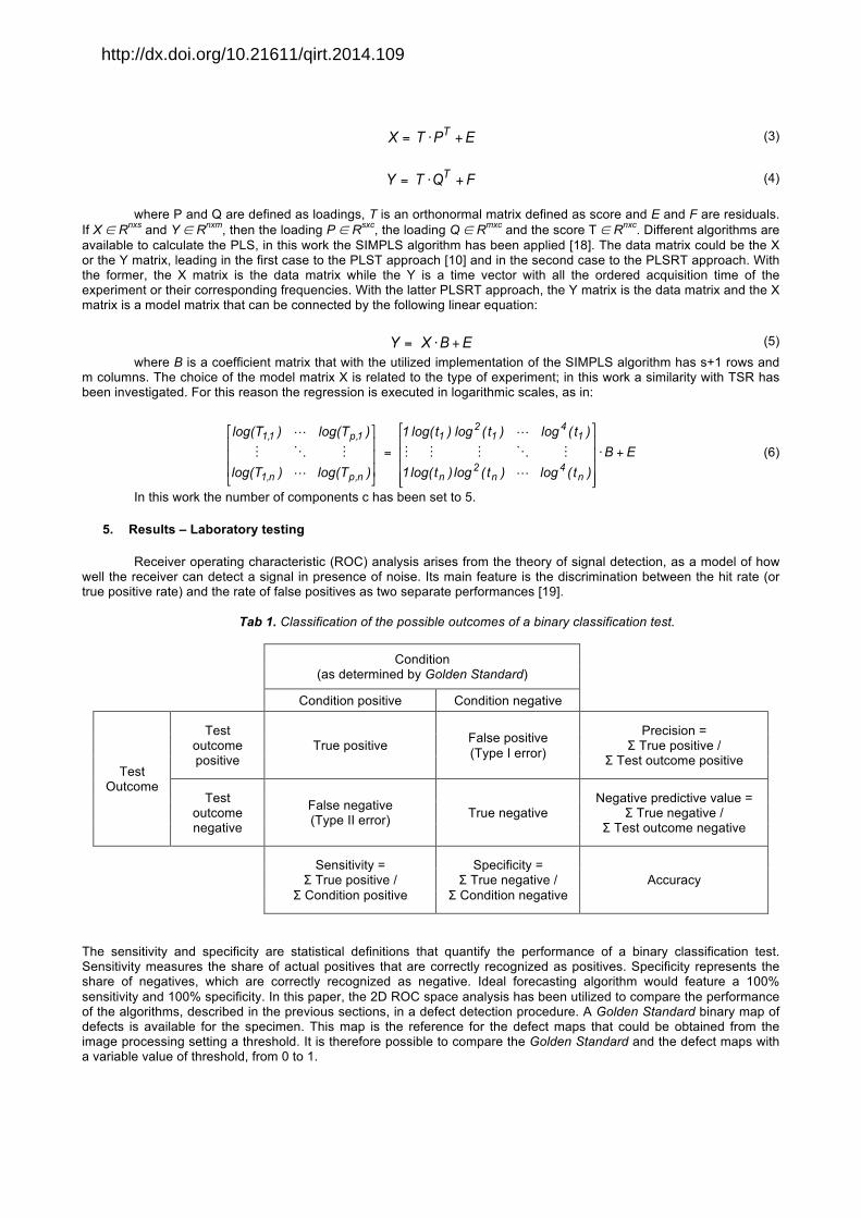
Tab 1. Classification of the possible outcomes of a binary classification test.

Condition (as determined by Golden Standard)

Condition positive Condition negative

Test Outcome

Test outcome positive

True positive False positive (Type I error)

Precision = Σ True positive /

Σ Test outcome positive

Test outcome negative

False negative (Type II error) True negative

Negative predictive value = Σ True negative /

Σ Test outcome negative

Sensitivity = Σ True positive /

Σ Condition positive

Specificity = Σ True negative /

Σ Condition negative Accuracy

The sensitivity and specificity are statistical definitions that quantify the performance of a binary classification test. Sensitivity measures the share of actual positives that are correctly recognized as positives. Specificity represents the share of negatives, which are correctly recognized as negative. Ideal forecasting algorithm would feature a 100% sensitivity and 100% specificity. In this paper, the 2D ROC space analysis has been utilized to compare the performance of the algorithms, described in the previous sections, in a defect detection procedure. A Golden Standard binary map of defects is available for the specimen. This map is the reference for the defect maps that could be obtained from the image processing setting a threshold. It is therefore possible to compare the Golden Standard and the defect maps with a variable value of threshold, from 0 to 1.


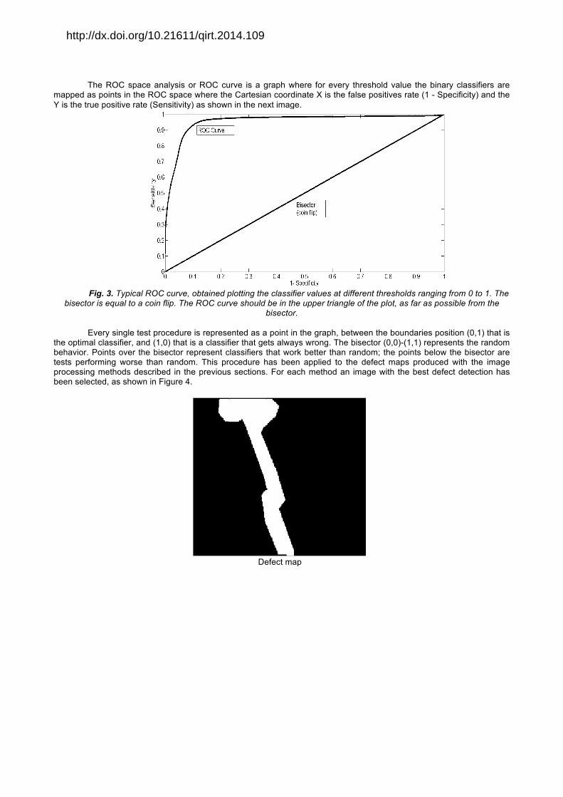
The ROC space analysis or ROC curve is a graph where for every threshold value the binary classifiers are mapped as points in the ROC space where the Cartesian coordinate X is the false positives rate (1 - Specificity) and the Y is the true positive rate (Sensitivity) as shown in the next image.

Fig. 3. Typical ROC curve, obtained plotting the classifier values at different thresholds ranging from 0 to 1. The

bisector is equal to a coin flip. The ROC curve should be in the upper triangle of the plot, as far as possible from the bisector.

Every single test procedure is represented as a point in the graph, between the boundaries position (0,1) that is

the optimal classifier, and (1,0) that is a classifier that gets always wrong. The bisector (0,0)-(1,1) represents the random behavior. Points over the bisector represent classifiers that work better than random; the points below the bisector are tests performing worse than random. This procedure has been applied to the defect maps produced with the image processing methods described in the previous sections. For each method an image with the best defect detection has been selected, as shown in Figure 4.

Defect map


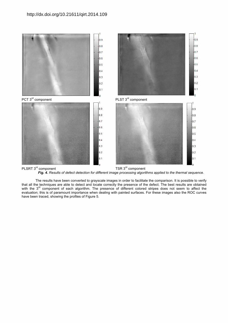
PCT 3rd component

PLST 3rd component

PLSRT 3rd component

TSR 3rd component

Fig. 4. Results of defect detection for different image processing algorithms applied to the thermal sequence. The results have been converted to grayscale images in order to facilitate the comparison. It is possible to verify

that all the techniques are able to detect and locate correctly the presence of the defect. The best results are obtained with the 3rd component of each algorithm. The presence of different colored stripes does not seem to affect the evaluation; this is of paramount importance when dealing with painted surfaces. For these images also the ROC curves have been traced, showing the profiles of Figure 5.


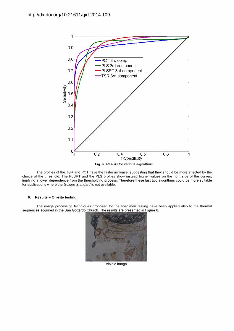
Fig. 5. Results for various algorithms.

The profiles of the TSR and PCT have the faster increase, suggesting that they should be more affected by the

choice of the threshold. The PLSRT and the PLS profiles show instead higher values on the right side of the curves, implying a lower dependence from the thresholding process. Therefore these last two algorithms could be more suitable for applications where the Golden Standard is not available.

6. Results – On-site testing

The image processing techniques proposed for the specimen testing have been applied also to the thermal sequences acquired in the San Gottardo Church. The results are presented in Figure 6.

Visible image


PCT 3rd component

PLST 3rd component

PLSRT 3nd component

TSR 3nd component

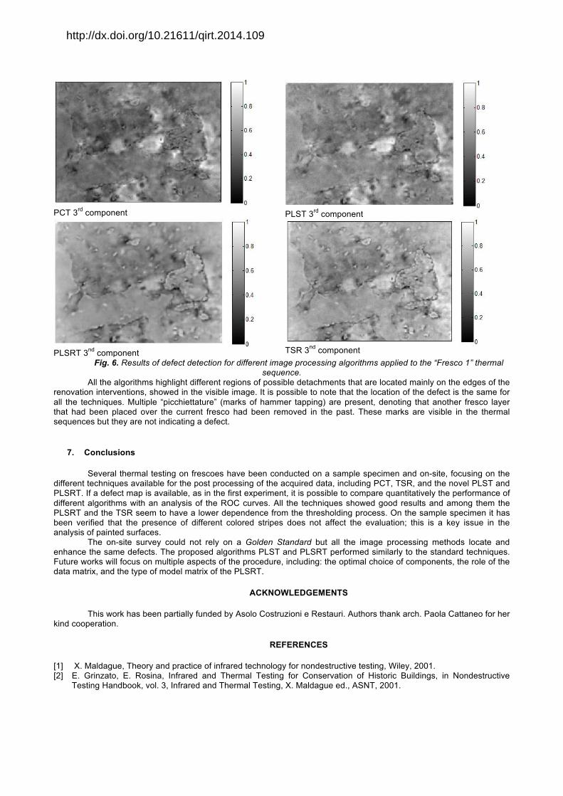
Fig. 6. Results of defect detection for different image processing algorithms applied to the “Fresco 1” thermal sequence.

All the algorithms highlight different regions of possible detachments that are located mainly on the edges of the renovation interventions, showed in the visible image. It is possible to note that the location of the defect is the same for all the techniques. Multiple “picchiettature” (marks of hammer tapping) are present, denoting that another fresco layer that had been placed over the current fresco had been removed in the past. These marks are visible in the thermal sequences but they are not indicating a defect.

7. Conclusions

Several thermal testing on frescoes have been conducted on a sample specimen and on-site, focusing on the different techniques available for the post processing of the acquired data, including PCT, TSR, and the novel PLST and PLSRT. If a defect map is available, as in the first experiment, it is possible to compare quantitatively the performance of different algorithms with an analysis of the ROC curves. All the techniques showed good results and among them the PLSRT and the TSR seem to have a lower dependence from the thresholding process. On the sample specimen it has been verified that the presence of different colored stripes does not affect the evaluation; this is a key issue in the analysis of painted surfaces.

The on-site survey could not rely on a Golden Standard but all the image processing methods locate and enhance the same defects. The proposed algorithms PLST and PLSRT performed similarly to the standard techniques. Future works will focus on multiple aspects of the procedure, including: the optimal choice of components, the role of the data matrix, and the type of model matrix of the PLSRT.

ACKNOWLEDGEMENTS

This work has been partially funded by Asolo Costruzioni e Restauri. Authors thank arch. Paola Cattaneo for her kind cooperation.

REFERENCES

[1] X. Maldague, Theory and practice of infrared technology for nondestructive testing, Wiley, 2001. [2] E. Grinzato, E. Rosina, Infrared and Thermal Testing for Conservation of Historic Buildings, in Nondestructive

Testing Handbook, vol. 3, Infrared and Thermal Testing, X. Maldague ed., ASNT, 2001.


[3] A. Bortolin, G. Cadelano, G. Ferrarini, P. Bison, F. Peron, X. Maldague, High-resolution survey of buildings by lock-in IR thermography, in: Thermosense: Thermal Infrared Applications XXXV, 2013: pp. 870503–870503–9. doi:10.1117/12.2016592.

[4] E. Grinzato, C. Bressan, S. Marinetti, P. Bison, C. Bonacina, Monitoring of the Scrovegni Chapel by IR thermography: Giotto at infrared, Infrared Physics & Technology 43(3–5), 165–169 (2002).

[5] J.L. Bodnar, K. Mouhoubi, L.D. Pallo, V. Detalle, J.M. Vallet, T. Duvaut, Contribution to the improvement of heritage mural painting non-destructive testing by stimulated infrared thermography, EPJ Applied Physics, 64 (1), art. no. 11001, (2013).

[6] C. Daffara, L. Pezzati, D. Ambrosini, D. Paoletti, R. Di Biase, P.I. Mariotti, C. Frosinini, Wide-band IR imaging in the NIR-MIR-FIR regions for in situ analysis of frescoes, Proceedings of SPIE - The International Society for Optical Engineering, 8084, art. no. 808406, (2011).

[7] G.M. Carlomagno, C. Meola, Comparison between thermographic techniques for frescoes NDT, NDT & E International. 35 (2002) 559–565. doi:10.1016/S0963-8695(02)00029-4.

[8] A. Bendada, S. Sfarra, D. Ambrosini, D. Paoletti, C. Ibarra-Castanedo, X. Maldague, Active thermography data processing for the NDT&E of frescoes, in: QIRT 10th International Conference on Quantitative InfraRed Thermography, Québec, Canada, 2010.

[9] C. Ibarra-Castanedo, A. Bendada, X. Maldague, Thermographic image processing for NDT, IV Conferencia Panamericana de END, Buenos Aires, Argentina, 2007.

[10] F. López, V.P..Vicente, X. Maldague, C. Ibarra-Castanedo, Multivariate Infrared Signal Processing by Partial Least-Squares Thermography, in: Québec, Canada, 2013.

[11] N. Rajic, Principal component thermography for flaw contrast enhancement and flaw depth characterisation in composite structures, Composite Structures. 58 (2002) 521–528. doi:10.1016/S0263-8223(02)00161-7.

[12] S. Marinetti, E. Grinzato, P. Bison, E. Bozzi, M. Chimenti, G. Pieri and O. Salvetti, Statistical analysis of IR thermographic sequences by PCA, Infrared Physics & Technology, vol. 46, p. 85–91, 2004.

[13] S. Marinetti, L. Finesso, E. Marsilio, Archetypes and principal components of an IR image sequence, Infrared Physics and Technology, 49 (3 SPEC. ISS.), pp. 272-276, (2007).

[14] S.M. Shepard, J.R. Lhota, B.A. Rubadeux, D. Wang, T. Ahmed, Reconstruction and enhancement of active thermographic image sequences, Opt. Eng. 42 ,1337–1342, (2003).

[15] S. Shepard, J. Hou, J. Lhota, and J. Golden. Automated processing of thermographic derivatives for quality assurance. Opt. Eng., 46(5), (2007).

[16] D. Balageas, Defense and illustration of time-resolved pulsed thermography for nde. QIRT Journal, 9(1):3–32, June 2012.

[17] H. Wold, Partial Least Squares, in: S. Kotz, N. Johnson (Eds.), Encyclopedia of Statistical Sciences, Wiley, New York, 1985.

[18] The MathWorks, Inc., MATLAB and Statistics Toolbox Release 2012b, The MathWorks, Inc., Natick, Massachusetts, United States., 2012.

[19] T. Fawcett, An Introduction to ROC Analysis, Pattern Recogn. Lett. 27 (2006) 861–874. doi:10.1016/j.patrec.2005.10.010.


Documents

Evaluation of frescoes detachments by partial least square