Embed Size (px)
Citation preview
Clemson UniversityTigerPrints
All Dissertations Dissertations
12-2009
Evaluation of Fluid Diodes as Pulmonary HeartValve ReplacementsTiffany CampClemson University, [email protected]
Follow this and additional works at: https://tigerprints.clemson.edu/all_dissertations
Part of the Engineering Mechanics Commons
This Dissertation is brought to you for free and open access by the Dissertations at TigerPrints. It has been accepted for inclusion in All Dissertations byan authorized administrator of TigerPrints. For more information, please contact [email protected].
Recommended CitationCamp, Tiffany, "Evaluation of Fluid Diodes as Pulmonary Heart Valve Replacements" (2009). All Dissertations. 497.https://tigerprints.clemson.edu/all_dissertations/497
EVALUATION OF FLUID DIODES FOR USE A PULMONARY HEART VALVE REPLACEMENTS
A Dissertation Presented to
the Graduate School of Clemson University
In Partial Fulfillment of the Requirements for the Degree
Doctor of Philosophy Mechanical Engineering
by Tiffany A. Camp December 2009
Accepted by: Richard Figliola, PhD, Committee Chair
Donald Beasley, PhD Martine LaBerge, PhD
TY Hsia, MD

ii
ABSTRACT
Children born with congenital heart disease often times suffer from severe chronic
pulmonary insufficiency. Palliative treatments for this condition may come early on in
the life of the patient; however, if it becomes severe enough, a pulmonary valve
replacement may be required. There currently is not a permanent option for a
replacements valve. Therefore, a need exists to develop a permanent solution. Knowing
that the right heart circulation is more tolerant of moderate levels of regurgitation (0 –
35%) and pressure gradient (0 – 30 mmHg), this study investigates the hypothesis that a
fluid diode, a motionless valve that offers low resistance to forward flow and high
resistance to reverse flow, could serve as a permanent solution.
The diode valve concept was tested in vitro in a mock pulmonary circulatory
system (MPCS). Transvalvular pressure gradient (TVG) and regurgitant fraction (RF%)
were used to assess valve performance. The valve was tested in vitro over a range of
pulmonary vascular resistances (PVR). In vivo testing was completed using a swine
model. A parametric study was also done to find the effect of changing geometries on
the flow regulating capabilities of the valves. Finally, flow field studies were performed
using particle image velocimetry (PIV). The flow patterns, viscous shear and Reynolds
shear stresses were analyzed, and the potential for platelet activation and thrombus
formation was determined.
iii
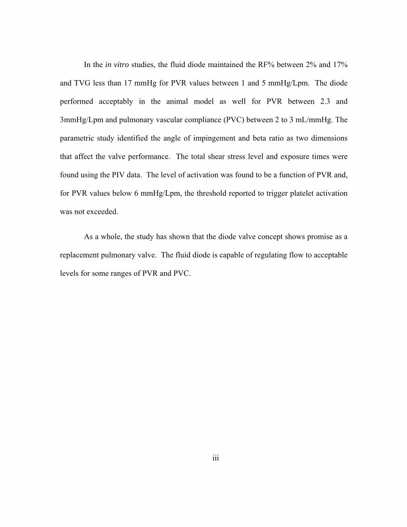
In the in vitro studies, the fluid diode maintained the RF% between 2% and 17%
and TVG less than 17 mmHg for PVR values between 1 and 5 mmHg/Lpm. The diode
performed acceptably in the animal model as well for PVR between 2.3 and
3mmHg/Lpm and pulmonary vascular compliance (PVC) between 2 to 3 mL/mmHg. The
parametric study identified the angle of impingement and beta ratio as two dimensions
that affect the valve performance. The total shear stress level and exposure times were
found using the PIV data. The level of activation was found to be a function of PVR and,
for PVR values below 6 mmHg/Lpm, the threshold reported to trigger platelet activation
was not exceeded.
As a whole, the study has shown that the diode valve concept shows promise as a
replacement pulmonary valve. The fluid diode is capable of regulating flow to acceptable
levels for some ranges of PVR and PVC.

iv
ACKNOWLEDGEMENTS
There are several people that I would like to acknowledge as without them, this
study would not have been possible. First, I would like to acknowledge those that
supported me financially during my doctoral studies. I must acknowledge the NSF
Graduate Research Fellowship program which supported me during my dissertation
research. I would like to also acknowledge the financial support of the Endowed
Teaching Fellows program in the Department of Mechanical Engineering at Clemson. I
would like to also acknowledge the NIH for their support of the research project.
Additionally, I must acknowledge The Timken Company, the South East Alliance for
Graduate Education and the Professoriate, and the PEER/WISE program at Clemson for
funding as well.
There were many people in the Department of Mechanical Engineering that I
would like to acknowledge. First, I must thank Jamie Cole, Michael Justice and Steven
Bass for their help in the machine shop and for putting up with me walking in at 4PM
every day. I would like to acknowledge those in Machining and Technical Services that
machined the fluid diodes used for testing. I would like to thank Linda, Renee, Kathryn,
Terri, Carol, Sara, Lindsey, Tameka and Gwen for all their support.
There were many undergraduate researchers whose work and help I would like to
acknowledge: Jeff Gohean, Kelley Stewart, Stephanie (Hequembourg) Waldrop, Brandon
Epperson, Dusty Coleman, Layne Madden and Maggie Zawaski.

v
I must acknowledge Dr. Tim Conover for his invaluable work in many different
areas on this project.
I would also like to acknowledge the staff and faculty at MUSC that assisted with
the animal studies. I would like to specifically acknowledge Dr. McQuinn for his help
and advice and Dr. Hsia for performing the surgeries.
I would like to acknowledge my committee members: Dr. Beasley, Dr. LaBerge
and Dr. Hsia. I thank you all for your interest in my research, the advice that you given
me, and numerous recommendation letters that you’ve written for me.
Of course, I must thank my advisor Dr, Figliola, for his knowledge, guidance,
time and patience throughout this process. I know I made it difficult at times.
Finally, I would like thank my family that have stood by me and put up with me
over the years. I would like to send thanks to my new, extended family at Peace for you
support and prayers. I would like to thank my fellow graduate students for
commiserating with me over the past few years. Thank you to Sue Lasser for listening
whenever about whatever. I would to thank all my friends, especially Heather Feldman,
Mary Holloway, Noelle Dietrich, Nancy Moore and Molly Rankin for their friendship
and advice. And thanks to Shell and Maggie for date night.
Words cannot express the appreciation and gratitude that I have for my partner,
Kim. Thank you for standing by me during this process. It means more to me than you
will know. OJ.
vi
TABLE OF CONTENTS
Page
TITLE PAGE ............................................................................................................... i
ABSTRACT ................................................................................................................ ii
ACKNOWLEDGEMENTS ....................................................................................... iv
LIST OF FIGURES .................................................................................................... ix
LIST OF TABLES ................................................................................................. xxix
NOMENCLATURE ............................................................................................... xxxi
CHAPTER
1. INTRODUCTION ................................................................................................... 1
2. BACKGROUND ..................................................................................................... 4
Pulmonary Circulation in a Healthy Heart ........................................... 4 Diseases of the Pulmonary Heart Valve ............................................... 7 Types of Replacement Valves .............................................................. 9 Effect of Shear Stress and Flow Anomalies ....................................... 17 Experimental Methods ....................................................................... 22 The Fluid Diode ................................................................................. 29
3. RESEARCH METHODS ...................................................................................... 37
Mock Pulmonary Circulatory System ................................................ 38 Global Flow and Pressure Measurements .......................................... 42 Optical Flow Field Measurements ..................................................... 44 Test Fluids .......................................................................................... 54
4. DIODE PERFORMANCE TESTING RESULTS ................................................ 55
Preliminary Testing ............................................................................ 55 5. ANIMAL MODEL RESULTS ............................................................................. 62
Introduction ........................................................................................ 62 Methods .............................................................................................. 62

vii
Table of Contents (Continued)
Page
Results ................................................................................................ 64 Summary ............................................................................................ 66
6. PARAMETRIC STUDY RESULTS ..................................................................... 69
Test conditions ................................................................................... 69 Results – Varying α and Inner Ring ................................................... 70 Results – Beta Ratio ........................................................................... 75
7. PARTICLE IMAGE VELOCIMETRY RESULTS .............................................. 80
Effect of Inertance .............................................................................. 80 Determination of Time Delays ........................................................... 82 Discussion of Data Sets ...................................................................... 83 Baseline PIV Data .............................................................................. 84 Open Cusped Diode Results ............................................................... 85 Back Channel Diode Results ............................................................ 120 Comparison of Backchannel and Open Cusped Diode Valves ...................................................................................... 148 Shear Stress Level and Exposure Time ............................................ 153 LDV Results ..................................................................................... 157
8. SUMMARY AND CONCLUSIONS .................................................................. 163
Summary of Results ......................................................................... 163 Conclusions ...................................................................................... 167 Recommendations ............................................................................ 167
APPENDICES ......................................................................................................... 169
APPENDIX A: Multi-Scale Model of the Fluid Diode in the Mock Circulatory System .............................................................. 170 APPENDIX B: PIV Results ......................................................................... 176
viii
Table of Contents (Continued)
Page
APPENDIX C: Uncertainty Analysis .......................................................... 232
REFERENCES ........................................................................................................ 237
ix
LIST OF FIGURES
Figure Page
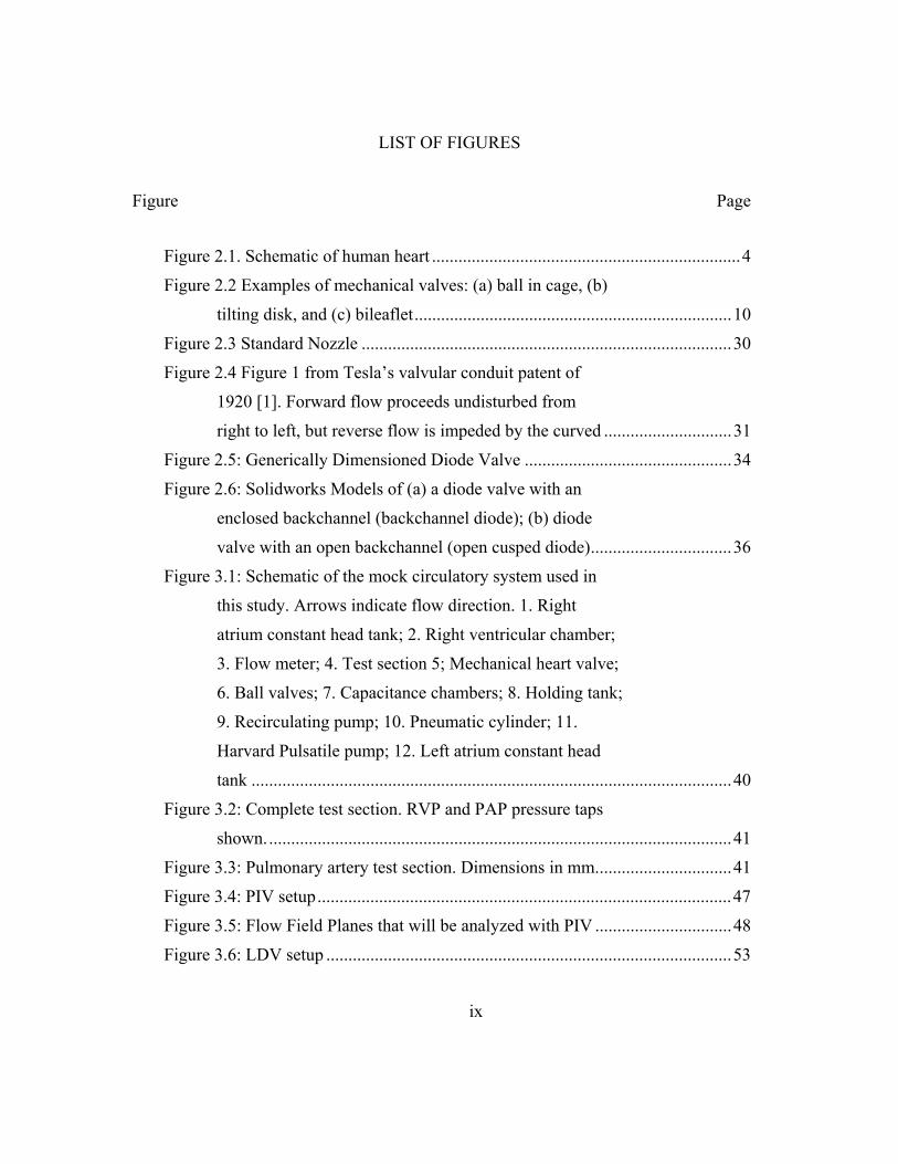
Figure 2.1. Schematic of human heart ...................................................................... 4
Figure 2.2 Examples of mechanical valves: (a) ball in cage, (b)
tilting disk, and (c) bileaflet ........................................................................ 10
Figure 2.3 Standard Nozzle .................................................................................... 30
Figure 2.4 Figure 1 from Tesla’s valvular conduit patent of
1920 [1]. Forward flow proceeds undisturbed from
right to left, but reverse flow is impeded by the curved ............................. 31
Figure 2.5: Generically Dimensioned Diode Valve ............................................... 34
Figure 2.6: Solidworks Models of (a) a diode valve with an
enclosed backchannel (backchannel diode); (b) diode
valve with an open backchannel (open cusped diode) ................................ 36
Figure 3.1: Schematic of the mock circulatory system used in
this study. Arrows indicate flow direction. 1. Right
atrium constant head tank; 2. Right ventricular chamber;
3. Flow meter; 4. Test section 5; Mechanical heart valve;
6. Ball valves; 7. Capacitance chambers; 8. Holding tank;
9. Recirculating pump; 10. Pneumatic cylinder; 11.
Harvard Pulsatile pump; 12. Left atrium constant head
tank ............................................................................................................. 40
Figure 3.2: Complete test section. RVP and PAP pressure taps
shown. ......................................................................................................... 41
Figure 3.3: Pulmonary artery test section. Dimensions in mm. .............................. 41
Figure 3.4: PIV setup .............................................................................................. 47
Figure 3.5: Flow Field Planes that will be analyzed with PIV ............................... 48
Figure 3.6: LDV setup ............................................................................................ 53

x
List of Figures (Continued)
Figure Page
Figure 4.1: Physiological signals using SJMBV (5 Lpm, 75 bpm,
3.9 mm Hg/Lpm) ........................................................................................ 57
Figure 4.2: Physiological signals using OTDV (5 Lpm, 75 bpm,
2.9 mm Hg/Lpm) ........................................................................................ 58
Figure 4.3: Physiological signals using diode (5 Lpm, 74 bpm,
3.1 mm Hg/Lpm) ........................................................................................ 58
Figure 4.4: Regurgitant Fraction (RF) and peak to peak
transvalvular gradient at 5 Lpm .................................................................. 59
Figure 5.1. Example flow and pressure curve collected during
animal tests using a 25 mm opencusped diode valve ................................. 66
Figure 5.2. PVR vs RF% for both the in vivo and in vitro tests.
In vitro test completed at 110 bpm, CO = 5 Lpm. ...................................... 67
Figure 5.3. TVG vs RF% for both the in vivo and in vitro tests.
In vitro test completed at 110 bpm, CO = 5 Lpm. ...................................... 68
Figure 5.4. PVR vs PVC for animal model and the in vitro ......................................
model with a 25 mm open cusped diode valve. .......................................... 68
Figure 6.1. Characteristic Resistance - Compliance Curve for
an Open Cusped Diode Valve ..................................................................... 70
Figure 6.2: PVR vs RF% and TVG (mmHg) for all
backchannel diode valves (β=0.50) with 95%
confidence intervals .................................................................................... 73
Figure 6.3: PVR vs RF% and TVG (mmHg) for all open
cupsed diode valves (β=0.50) with 95% confidence
intervals ....................................................................................................... 73
Figure 6.4: PVR vs RF% and TVG (mmHg) for diode valves
with α = 60˚ (β=0.50) with 95% confidence intervals ................................ 77
xi
List of Figures (Continued)
Figure Page
Figure 6.5: PVR vs RF% and TVG (mmHg) for diode valves
with α = 75˚ (β=0.50) with 95% confidence intervals ................................ 77
Figure 6.6: PVR vs RF% and TVG (mmHg) for diode valves
with α = 90˚ (β=0.50) with 95% confidence intervals ................................ 78
Figure 6.7: PVR vs TVG for open cusped diode valve with
different beta ratios. 95% confidence interval included.
Tests conducted at cardiac output of 4 Lpm. .............................................. 78
Figure 6.8: PVR vs RF% for open cusped diodes valve with
different beta ratios. 95% confidence intervals included. ........................... 79
Figure 7.1. Lumped parameter model for the upstream of the
Mock Circulatory System. .......................................................................... 82
Figure 7.2 Coverage area for the (a) Central PIV plane and (b)
offset PIV planes ......................................................................................... 84
Figure 7.3. Flow and Pressure curve for PVR = 3.1mmHg/Lpm ........................... 88
Figure 7.4. Central plane flow and viscous shear stress
(dynes/cm2) field for the open cusped diode at 150 ms
after the start of systole for PVR = 3.1 Lpm ............................................... 88
Figure 7.5: Reynolds shear stress field (dynes/cm2) for the open
cusped diode at 150 ms after the start of systole for PVR
= 3.1 mmHg/Lpm, central plane ................................................................ 89
Figure 7.6: Central plane flow and viscous shear stress
(dynes/cm2) field for the open cusped diode at 350 ms ................................
after the start of systole for PVR = 3.1 Lpm ............................................... 91
Figure 7.7: Reynolds shear stress field (dynes/cm2) for the
open cusped diode at 350 ms after the start of systole
for PVR = 3.1 mmHg/Lpm, central plane .................................................. 91

xii
List of Figures (Continued)
Figure Page
Figure 7.8. Central plane flow and viscous shear stress
(dynes/cm2) field for the open cusped diode at 550 ms
after the start of systole for PVR = 3.1 Lpm ............................................... 93
Figure 7.9: Reynolds shear stress field (dynes/cm2) for the open
cusped diode at 550 ms after the start of systole for PVR
= 3.1 mmHg/Lpm, central plane ................................................................ 93
Figure 7.10. Central plane flow and viscous shear stress
(dynes/cm2) field for the open cusped diode at 750 ms
after the start of systole for PVR = 3.1 Lpm ............................................... 94
Figure 7.11: Reynolds shear stress field (dynes/cm2) for the
open cusped diode at 750 ms after the start of systole
for PVR = 3.1 mmHg/Lpm, central plane .................................................. 94
Figure 7.12. Offset plane flow and viscous shear stress
(dynes/cm2) field for the open cusped diode at 150 ms
after the start of systole for PVR = 3.1 Lpm ............................................... 97
Figure 7.13: Reynolds shear stress field (dynes/cm2) for the
open cusped diode at 150 ms after the start of systole
for PVR = 3.1 mmHg/Lpm, offset plane .................................................... 98
Figure 7.14. Offset plane flow and viscous shear stress
(dynes/cm2) field for the open cusped diode at 350 ms
after the start of systole for PVR = 3.1 Lpm ............................................... 98
Figure 7.15:Reynolds shear stress field (dynes/cm2) for the
open cusped diode at 350 ms after the start of systole for
PVR = 3.1 mmHg/Lpm, offset plane .......................................................... 99
xiii
List of Figures (Continued)
Figure Page
Figure 7.16. Offset plane flow and viscous shear stress
(dynes/cm2) field for the open cusped diode at 550 ms
after the start of systole for PVR = 3.1 Lpm ............................................... 99
Figure 7.17: Reynolds shear stress field (dynes/cm2) for the
open cusped diode at 550 ms after the start of systole for
PVR = 3.1 mmHg/Lpm, offset plane ........................................................ 100
Figure 7.18. Offset plane flow and viscous shear stress
(dynes/cm2) field for the open cushed diode at 750 ms
after the start of systole for PVR = 3.1 Lpm ............................................. 100
Figure 7.19: Reynolds shear stress field (dynes/cm2) for the
open cusped diode at 750 ms after the start of systole
for PVR = 3.1 mmHg/Lpm, offset plane .................................................. 101
Figure 7.20: Flow and pressure curves for the open cusped
diode, PVR = 5.1 mmHg/Lpm .................................................................. 101
Figure 7.21: Central plane flow and viscous shear stress
(dynes/cm2) field for the open cusped diode at 150 ms
after the start of systole for PVR = 5.1 mmHg/Lpm ................................ 103
Figure 7.22: Reynolds shear stress field (dynes/cm2) for the
open cusped diode at 150 ms after the start of systole for
PVR = 5.1 mmHg/Lpm, central plane ...................................................... 103
Figure 7.23: Central plane flow and viscous shear stress
(dynes/cm2) field for the open cusped diode at 350 ms
after the start of systole for PVR = 5.1 mmHg/Lpm ................................ 105
Figure 7.24: Reynolds shear stress field (dynes/cm2) for the
open cusped diode at 350 ms after the start of systole for
PVR = 5.1 mmHg/Lpm, central plane ...................................................... 105

xiv
List of Figures (Continued)
Figure Page
Figure 7.25: Central plane flow and viscous shear stress
(dynes/cm2) field for the open cusped diode at 450 ms
after the start of systole (peak) for PVR = 5.1 mmHg/Lpm ..................... 107
Figure 7.26: Reynolds shear stress (dynes/cm2) field for the
open cusped diode at 450 ms after the start of systole
(peak) for PVR = 5.1 mmHg/Lpm ............................................................ 107
Figure 7.27: Central plane flow and viscous shear stress
(dynes/cm2) field for the open cusped diode at 550 ms
after the start of systole for PVR = 5.1 mmHg/Lpm ................................ 110
Figure 7.28: Reynolds shear stress field (dynes/cm2) for the
open cusped diode at 550 ms after the start of systole
for PVR = 5.1 mmHg/Lpm, central plane ................................................ 110
Figure 7.29: Central plane flow and viscous shear stress
(dynes/cm2) field for the open cusped diode at 750 ms
after the start of systole for PVR = 5.1 mmHg/Lpm ................................ 111
Figure 7.30: Reynolds shear stress field (dynes/cm2) for the
open cusped diode at 750 ms after the start of systole
for PVR = 5.1 mmHg/Lpm, central plane ................................................ 111
Figure 7.31: Pressure and flow curve for the open cusped diode
at PVR = 6.1 mmHg/Lpm ......................................................................... 112
Figure 7.32: Central plane flow and viscous shear stress
(dynes/cm2) field for the open cusped diode at 150 ms
after the start of systole for PVR 6.1 mmHg/Lpm .................................... 115
Figure 7.33: Reynolds shear stress (dynes/cm2) field for the
open cusped diode at 150 ms after the start of systole
for PVR = 6.1 mmHg/Lpm ....................................................................... 115

xv
List of Figures (Continued)
Figure Page
Figure 7.34: Central plane flow and viscous shear stress
(dynes/cm2) field for the open cusped diode at 350 ms
after the start of systole for PVR 6.1 mmHg/Lpm .................................... 116
Figure 7.35: Reynolds shear stress (dynes/cm2) field for the
open cusped diode at 350 ms after the start of systole
for PVR = 6.1 mmHg/Lpm ....................................................................... 116
Figure 7.36: Central plane flow and viscous shear stress
(dynes/cm2) field for the open cusped diode at 550 ms
after the start of systole for PVR 6.1 mmHg/Lpm .................................... 118
Figure 7.37: Reynolds shear stress (dynes/cm2) field for the
open cusped diode at 550 ms after the start of systole
for PVR = 6.1 mmHg/Lpm ....................................................................... 118
Figure 7.38: Central plane flow and viscous shear stress
(dynes/cm2) field for the open cusped diode at 750 ms
after the start of systole for PVR 6.1 mmHg/Lpm .................................... 119
Figure 7.39: Reynolds shear stress (dynes/cm2) field for the
open cusped diode at 750 ms after the start of systole
for PVR = 6 .1mmHg/Lpm ....................................................................... 119
Figure 7.40: Pressure and flow curve for backchannel diode at
PVR = 3.2 mmHg/Lpm ............................................................................ 122
Figure 7.41: Central plane flow and viscous shear stress
(dynes/cm2) field for the backchannel diode at 150 ms
after the start of systole for PVR = 3.2 mmHg/Lpm ................................ 122
Figure 7.42: Reynolds shear stress field (dynes/cm2) for the
backchannel diode at 150 ms after the start of systole
for PVR = 3.2 mmHg/Lpm, central plane ................................................ 123

xvi
List of Figures (Continued)
Figure Page
Figure 7.43: Central plane flow and viscous shear stress
(dynes/cm2) field for the backchannel diode at 350 ms
after the start of systole for PVR = 3.2 mmHg/Lpm ................................ 125
Figure 7.44: Reynolds shear stress field (dynes/cm2) for the
backchannel diode at 350 ms after the start of systole
for PVR = 3.2 mmHg/Lpm, central plane ................................................ 126
Figure 7.45: Central plane flow and viscous shear stress
(dynes/cm2) field for the backchannel diode at 550 ms
after the start of systole for PVR = 3.2 mmHg/Lpm ................................ 126
Figure 7.46: Reynolds shear stress field (dynes/cm2) for the
backchannel diode at 550 ms after the start of systole
for PVR = 3.2 mmHg/Lpm, central plane ................................................ 127
Figure 7.47: Central plane flow and viscous shear stress
(dynes/cm2) field for the backchannel diode at 750 ms
after the start of systole for PVR = 3.2 mmHg/Lpm ................................ 127
Figure 7.48: Reynolds shear stress field (dynes/cm2) for the
backchannel diode at 750 ms after the start of systole
for PVR = 3.2 mmHg/Lpm, central plane ................................................ 128
Figure 7.49: Offset plane flow and viscous shear stress
(dynes/cm2) field at 150 ms after start of systole for
backchannel diode at PVR = 3.2 mmHg/Lpm .......................................... 130
Figure 7.50: Offset Reynolds shear stress (dynes/cm2) field at
150 ms after start of systole for backchannel diode at
PVR = 3.2 mmHg/Lpm ............................................................................ 130

xvii
List of Figures (Continued)
Figure Page
Figure 7.51: Offset plane flow and viscous shear stress
(dynes/cm2) field at 350 ms after start of systole for
backchannel diode at PVR = 3.2 mmHg/Lpm .......................................... 131
Figure 7.52: Offset Reynolds shear stress (dynes/cm2) field at
350 ms after start of systole for backchannel diode at
PVR = 3.2 mmHg/Lpm ............................................................................ 131
Figure 7.53: Offset plane flow and viscous shear stress
(dynes/cm2) field at 550 ms after start of systole for
backchannel diode at PVR = 3.2 mmHg/Lpm .......................................... 132
Figure 7.54: Offset Reynolds shear stress (dynes/cm2) field at
550 ms after start of systole for backchannel diode at
PVR = 3.2 mmHg/Lpm ............................................................................ 133
Figure 7.55: Offset plane flow and viscous shear stress
(dynes/cm2) field at 750 ms after start of systole for
backchannel diode at PVR = 3.2 mmHg/Lpm .......................................... 133
Figure 7.56: Offset Reynolds shear stress (dynes/cm2) field at
750 ms after start of systole for backchannel diode at
PVR = 3.2 mmHg/Lpm ............................................................................ 134
Figure 7.57: Offset plane flow and viscous shear stress
(dynes/cm2) field at 150 ms after start of systole for
backchannel diode at PVR = 5.1 mmHg/Lpm .......................................... 136
Figure 7.58: Offset Reynolds shear stress (dynes/cm2) field at
150 ms after start of systole for backchannel diode at
PVR = 5.1 mmHg/Lpm ............................................................................ 137
xviii
List of Figures (Continued)
Figure Page
Figure 7.59: Offset plane flow and viscous shear stress
(dynes/cm2) field at 350 ms after start of systole for
backchannel diode at PVR = 5.1 mmHg/Lpm .......................................... 137
Figure 7.60: Offset Reynolds shear stress (dynes/cm2) field at
350 ms after start of systole for backchannel diode at
PVR = 5.1 mmHg/Lpm ............................................................................ 138
Figure 7.61: Offset plane flow and viscous shear stress
(dynes/cm2) field at 550 ms after start of systole for
backchannel diode at PVR = 5.1 mmHg/Lpm .......................................... 138
Figure 7.62: Offset Reynolds shear stress (dynes/cm2) field at
550 ms after start of systole for backchannel diode at
PVR = 5.1 mmHg/Lpm ............................................................................ 139
Figure 7.63: Offset plane flow and viscous shear stress
(dynes/cm2) field at 750 ms after start of systole for
backchannel diode at PVR = 5.1 mmHg/Lpm .......................................... 139
Figure 7.64: Offset Reynolds shear stress (dynes/cm2) field at
750 ms after start of systole for backchannel diode at
PVR = 5.1 mmHg/Lpm ............................................................................ 140
Figure 7.65: Pressure and flow curve for backchannel diode at
PVR = 6.9 mmHg/Lpm ............................................................................ 141
Figure 7.66: Central plane flow and viscous shear stress
(dynes/cm2) field for the backchannel diode at 150 ms
after the start of systole for PVR 6.9 mmHg/Lpm .................................... 142
Figure 7.67: Reynolds shear stress (dynes/cm2) field for the
backchannel diode at 150 ms after the start of systole
for PVR = 6.9 mmHg/Lpm ....................................................................... 142

xix
List of Figures (Continued)
Figure Page
Figure 7.68: Central plane flow and viscous shear stress
(dynes/cm2) field for the backchannel diode at 350 ms
after the start of systole for PVR 6.9 mmHg/Lpm .................................... 144
Figure 7.69: Reynolds shear stress (dynes/cm2) field for the
backchannel diode at 350 ms after the start of systole
for PVR = 6.9 mmHg/Lpm ....................................................................... 144
Figure 7.70: Central plane flow and viscous shear stress
(dynes/cm2) field for the backchannel diode at 550 ms
after the start of systole for PVR 6.9 mmHg/Lpm .................................... 146
Figure 7.71: Reynolds shear stress (dynes/cm2) field for the
backchannel diode at 550 ms after the start of systole
for PVR = 6.9 mmHg/Lpm ....................................................................... 147
Figure 7.72: Central plane flow and viscous shear stress
(dynes/cm2) field for the backchannel diode at 750 ms
after the start of systole for PVR 6.9 mmHg/Lpm .................................... 147
Figure 7.73: Reynolds shear stress (dynes/cm2) field for the
backchannel diode at 750 ms after the start of systole
for PVR = 6.9 mmHg/Lpm ....................................................................... 148
Figure 7.74. Total shear stress field and three streamlines for
backchannel diode at PVR = 6.85 mmHg/Lpm 350 ms
after the start of systole. ............................................................................ 155
Figure 7.75. Positioning Grid of Data Points ....................................................... 158
Figure 7.76. Spectrum 28 mm Downstream of Backchannel
Diode Valve, 6mm above centerline ........................................................ 160
Figure 7.77. Spectrum 32 mm Downstream of Backchannel
Diode Valve, 6 mm above centerline ....................................................... 162
xx
List of Figures (Continued)
Figure Page
Figure A.1. Lumped parameter model for the upstream of the
Mock Circulatory System. ........................................................................ 171
Figure A.2. Lumped parameter model for the fluid diode, and
the downstream pulmonary impedance. ................................................... 172
Figure B.1: Flow and pressure curves for the open cusped
diode ......................................................................................................... 180
Figure B.2: Central plane flow and viscous shear stress
(dynes/cm2) field for the open cusped diode at 150 ms
after the start of systole for PVR = 4.3 mmHg/Lpm ................................ 180
Figure B.3: Reynolds shear stress field (dynes/cm2) for the open
cusped diode at 150 ms after the start of systole for
PVR = 4.3 mmHg/Lpm, central plane ...................................................... 181
Figure B.4: Central plane flow and viscous shear stress
(dynes/cm2) field for the open cusped diode at 350 ms
after the start of systole for PVR = 4.3 mmHg/Lpm ................................ 181
Figure B.5: Reynolds shear stress field (dynes/cm2) for the open
cusped diode at 350 ms after the start of systole for PVR
= 4.3 mmHg/Lpm, central plane ............................................................... 182
Figure B.6: Central plane flow and viscous shear stress
(dynes/cm2) field for the open cusped diode at 550 ms
after the start of systole for PVR = 4.3 mmHg/Lpm ................................ 182
Figure B.7: Reynolds shear stress field (dynes/cm2) for the open
cusped diode at 550 ms after the start of systole for PVR
= 4.3 mmHg/Lpm, central plane ............................................................... 183
xxi
List of Figures (Continued)
Figure Page
Figure B.8: Central plane flow and viscous shear stress
(dynes/cm2) field for the open cusped diode at 750 ms
after the start of systole for PVR = 4.3 mmHg/Lpm ................................ 183
Figure B.9: Reynolds shear stress field (dynes/cm2) for the open
cusped diode at 750 ms after the start of systole for
PVR= 4.3 mmHg/Lpm, central plane ....................................................... 186
Figure B.10: Offset plane flow and viscous shear stress
(dynes/cm2) field at 150 ms after start of systole for the
open cusp diode at PVR = 4.3 mmHg/Lpm .............................................. 186
Figure B.11: Offset Reynolds shear stress (dynes/cm2) field at
150 ms after start of systole for the open cusped diode
at PVR = 4.3 mmHg/Lpm ......................................................................... 187
Figure B.12: Offset plane flow and viscous shear stress
(dynes/cm2) field at 350 ms after start of systole for the
open cusp diode at PVR = 4.3 mmHg/Lpm .............................................. 187
Figure B.13: Offset Reynolds shear stress (dynes/cm2) field at
350 ms after start of systole for the open cusped diode
at PVR = 4.3 mmHg/Lpm ......................................................................... 188
Figure B.14: Offset plane flow and viscous shear stress
(dynes/cm2) field at 550 ms after start of systole for the
open cusp diode at PVR = 4.3 mmHg/Lpm .............................................. 188
Figure B.15: Offset Reynolds shear stress (dynes/cm2) field at
550 ms after start of systole for the open cusped diode
at PVR = 4.3 mmHg/Lpm ......................................................................... 189
xxii
List of Figures (Continued)
Figure Page
Figure B.16: Offset plane flow and viscous shear stress
(dynes/cm2) field at 750 ms after start of systole for the
open cusp diode at PVR = 4.3 mmHg/Lpm .............................................. 189
Figure B.17: Offset Reynolds shear stress (dynes/cm2) field at
750 ms after start of systole for the open cusped diode
at PVR = 4.3 mmHg/Lpm ......................................................................... 190
Figure B.18: Offset plane flow and viscous shear stress
(dynes/cm2) field for the open cusped diode at 150 ms
after start of systole at PVR = 5.1 mmHg/Lpm ........................................ 191
Figure B.19: Offset Reynolds shear stress (dynes/cm2) field for
the open cusped diode at 150 ms after start at PVR =
5.1 mmHg/Lpm ......................................................................................... 192
Figure B.20: Offset plane flow and viscous shear stress
(dynes/cm2) field for the open cusped diode at 350 ms
after start of systole at PVR = 5.1 mmHg/Lpm ........................................ 193
Figure B.21: Offset Reynolds shear stress (dynes/cm2) field for
the open cusped diode at 350 ms after start of systole at
PVR = 5.1 mmHg/Lpm ............................................................................ 194
Figure B.22: Offset plane flow and viscous shear stress
(dynes/cm2) field for the open cusped diode at 450 ms
after start of systole at PVR = 5.1 mmHg/Lpm ........................................ 195
Figure B.23: Offset Reynolds shear stress (dynes/cm2) field for
the open cusped diode at 450 ms after start of systole at
PVR = 5.1 mmHg/Lpm ............................................................................ 196
xxiii
List of Figures (Continued)
Figure Page
Figure B.24: Offset plane flow and viscous shear stress
(dynes/cm2) field for the open cusped diode at 550 ms
after start of systole at PVR = 5.1 mmHg/Lpm ........................................ 197
Figure B.25: Offset Reynolds shear stress (dynes/cm2) field for
the open cusped diode at 550 ms after start of systole at
PVR = 5.1 mmHg/Lpm ............................................................................ 197
Figure B.26: Offset plane flow and viscous shear stress
(dynes/cm2) field for the open cusped diode at 750 ms
after start of systole at PVR = 5.1 mmHg/Lpm ........................................ 198
Figure B.27: Offset Reynolds shear stress (dynes/cm2) field for
the open cusped diode at 750 ms after start of systole at
PVR = 5.1 mmHg/Lpm ............................................................................ 199
Figure B.28: Offset plane flow and viscous shear stress
(dynes/cm2) field for the open cusped diode at 150 ms
after the start of systole for PVR 6.1 mmHg/Lpm .................................... 200
Figure B.29: Offset Reynolds shear stress (dynes/cm2) field for
the open cusped diode at 150 ms after start of systole for
open cusped diode at PVR = 6.1 mmHg/Lpm .......................................... 200
Figure B.30: Offset plane flow and viscous shear stress
(dynes/cm2) field for the open cusped diode at 350 ms
after the start of systole for PVR 6.1 mmHg/Lpm .................................... 203
Figure B.31: Offset Reynolds shear stress (dynes/cm2) field for
the open cusped diode at 350 ms after start of systole for
open cusped diode at PVR = 6.1 mmHg/Lpm .......................................... 203
xxiv
List of Figures (Continued)
Figure Page
Figure B.32: Offset plane flow and viscous shear stress
(dynes/cm2) field for the open cusped diode at 550 ms
after the start of systole for PVR 6.1 mmHg/Lpm .................................... 204
Figure B.33: Offset Reynolds shear stress (dynes/cm2) field for
the open cusped diode at 550 ms after start of systole for
open cusped diode at PVR = 6.1 mmHg/Lpm .......................................... 204
Figure B.34: Offset plane flow and viscous shear stress
(dynes/cm2) field for the open cusped diode at 750 ms
after the start of systole for PVR 6.1 mmHg/Lpm .................................... 205
Figure B.35: Offset Reynolds shear stress (dynes/cm2) field for
the open cusped diode at 750 ms after start of systole
for open cusped diode at PVR = 6.1 mmHg/Lpm .................................... 205
Figure B.36: Flow and pressure curve for backchannel diode at
PVR 4.1 mmHg/Lpm ................................................................................ 206
Figure B.37: Central plane flow and viscous shear stress
(dynes/cm2) field for the backchannel diode at 150 ms
after the start of systole for PVR = 4.1 mmHg/Lpm ................................ 207
Figure B.38: Reynolds shear stress field (dynes/cm2) for the
backchannel diode at 150 ms after the start of systole
for PVR = 4.1 mmHg/Lpm, central plane ................................................ 206
Figure B.39: Central plane flow and viscous shear stress
(dynes/cm2) field for the backchannel diode at 350 ms
after the start of systole for PVR = 4.1 mmHg/Lpm ................................ 206
Figure B.40: Reynolds shear stress (dynes/cm2) field for the
backchannel diode at 350 ms after the start of systole
for PVR = 4.1 mmHg/Lpm, central plane ................................................ 208
xxv
List of Figures (Continued)
Figure Page
Figure B.41: Central plane flow and viscous shear stress
(dynes/cm2) field for the backchannel diode at 550 ms
after the start of systole for PVR = 4.1 mmHg/Lpm ................................ 208
Figure B.42: Reynolds shear stress (dynes/cm2) field for the
backchannel diode at 550 ms after the start of systole
for PVR = 4.1 mmHg/Lpm, central plane ................................................ 209
Figure B.43: Central plane flow and viscous shear stress
(dynes/cm2) field for the backchannel diode at 750 ms
after the start of systole for PVR = 4.1 mmHg/Lpm ................................ 212
Figure B.44: Reynolds shear stress (dynes/cm2) field for the
backchannel diode at 750 ms after the start of systole
for PVR = 4.1 mmHg/Lpm ....................................................................... 212
Figure B.45: Offset plane flow and viscous shear stress
(dynes/cm2) field at 150 ms after start of systole for
backchannel diode at PVR = 4.1 mmHg/Lpm .......................................... 213
Figure B.46: Offset Reynolds shear stress (dynes/cm2) field at
150 ms after start of systole for backchannel diode at
PVR = 4.1 mmHg/Lpm ............................................................................ 213
Figure B.47: Offset plane flow and viscous shear stress
(dynes/cm2) field at 350 ms after start of systole for
backchannel diode at PVR = 4.1 mmHg/Lpm .......................................... 214
Figure B.48: Offset Reynolds shear stress (dynes/cm2) field at
350 ms after start of systole for backchannel diode at
PVR = 4.1 mmHg/Lpm ............................................................................ 215

xxvi
List of Figures (Continued)
Figure Page
Figure B.49: Offset plane flow and viscous shear stress
(dynes/cm2) field at 550 ms after start of systole for
backchannel diode at PVR = 4.1 mmHg/Lpm .......................................... 215
Figure B.50: Offset Reynolds shear stress (dynes/cm2) field at
550 ms after start of systole for backchannel diode at
PVR = 4.1 mmHg/Lpm ............................................................................ 216
Figure B.51: Offset plane flow and viscous shear stress
(dynes/cm2) field at 750 ms after start of systole for
backchannel diode at PVR = 4.1 mmHg/Lpm .......................................... 216
Figure B.52: Offset Reynolds shear stress (dynes/cm2) field at
750 ms after start of systole for backchannel diode at
PVR = 4.1 mmHg/Lpm ............................................................................ 217
Figure B.53: Flow and Pressure Curve for backchannel diode
at PVR = 5.1 mmHg/Lpm ........................................................................ 218
Figure B.54: Central plane flow and viscous shear stress
(dynes/cm2) field for the backchannel diode at 150 ms
after the start of systole for PVR =5.1 mmHg/Lpm ................................. 219
Figure B.55: Reynolds shear stress (dynes/cm2) field for the
backchannel diode at 150 ms after the start of systole
for PVR = 5.1 mmHg/Lpm ....................................................................... 219
Figure B.56: Central plane flow and viscous shear stress
(dynes/cm2) field for the backchannel diode at 350 ms
after the start of systole for PVR = 5.1 mmHg/Lpm ................................ 221
Figure B.57: Central plane Reynolds shear stress (dynes/cm2)
field for the backchannel diode at 350 ms after the start
of systole for PVR = 5.1 mmHg/Lpm ...................................................... 221

xxvii
List of Figures (Continued)
Figure Page
Figure B.58: Central plane flow and viscous shear stress
(dynes/cm2) field for the backchannel diode at 550 ms
after the start of systole for PVR = 5.1 mmHg/Lpm ................................ 223
Figure B.59: Reynolds shear stress (dynes/cm2) field for the
backchannel diode at 550 ms after the start of systole
for PVR = 5.1 mmHg/Lpm ....................................................................... 223
Figure B.60: Central plane flow and viscous shear stress
(dynes/cm2) field for the backchannel diode at 750 ms
after the start of systole for PVR = 5.1 mmHg/Lpm ................................ 225
Figure B.61: Reynolds shear stress (dynes/cm2) field for the
backchannel diode at 750 ms after the start of systole
for PVR = 5.1 mmHg/Lpm, central plane ................................................ 225
Figure B.62: Offset plane flow and viscous shear stress
(dynes/cm2) field for the backchannel diode at 150 ms
after the start of systole for PVR 6.9 mmHg/Lpm .................................... 229
Figure B.63: Offset Reynolds shear stress (dynes/cm2) field at
150 ms after start of systole for backchannel diode at
PVR = 6.9 mmHg/Lpm ............................................................................ 229
Figure B.64: Offset plane flow and viscous shear stress
(dynes/cm2) field for the backchannel diode at 350 ms
after the start of systole for PVR 6.9 mmHg/Lpm .................................... 229
Figure B.65: Offset Reynolds shear stress (dynes/cm2) field at
350 ms after start of systole for backchannel diode at
PVR = 6.9 mmHg/Lpm ............................................................................ 230

xxviii
List of Figures (Continued)
Figure Page
Figure B.66: Offset plane flow and viscous shear stress
(dynes/cm2) field for the backchannel diode at 550 ms
after the start of systole for PVR 6.9 mmHg/Lpm .................................... 230
Figure B.67: Offset Reynolds shear stress (dynes/cm2) field at
550 ms after start of systole for backchannel diode at
PVR = 6.9 mmHg/Lpm ............................................................................ 231
Figure B.68: Offset plane flow and viscous shear stress
(dynes/cm2) field for the backchannel diode at 750 ms
after the start of systole for PVR 6.9 mmHg/Lpm .................................... 231
Figure B.69: Offset Reynolds shear stress (dynes/cm2) field at
750 ms after start of systole for backchannel diode at
PVR = 6.9 mmHg/Lpm ............................................................................ 232

xxix
LIST OF TABLES
Table Page
Table 2.1: Diode Design Dimensions ..................................................................... 36
Table 3.1. The Root Mean Squared of the velocity components
for increasing number of image pairs. ........................................................ 50
Table 4.1: Summary of effective orifice area (5 Lpm and
75 bpm) ....................................................................................................... 59
Table 5.1. Select Results from the Animal Model Testing with
95% Confidence Intervals ........................................................................... 65
Table 7.1. Comparison PIV Results for Backchannel (PVR =
3.2 mmHg/Lpm) and ................................................................................ 149
Table 7.2. Comparison PIV Results for Backchannel (PVR =
4.3 mmHg/Lpm) and Open Cusped (PVR = 4.2
mmHg/Lpm Diode Valves ........................................................................ 150
Table 7.3. Comparison PIV Results for Backchannel (PVR =
5.1 mmHg/Lpm) and Open Cusped (PVR = 5.1
mmHg/Lpm) Diode Valves ...................................................................... 151
Table 7.4. Comparison PIV Results for Backchannel (PVR =
6.9 mmHg/Lpm) and Open Cusped (PVR = 6.1
mmHg/Lpm) Diode Valves ...................................................................... 152
Table 7.5. The level of activation and average total shear for 3
streamlines for the backchannel diode at all PVR
(mmHg/Lpm) levels. ................................................................................. 156
Table A.1. Results from LPM Tests ..................................................................... 175
Table C. 1. Standard systematic uncertainties (b), random
uncertainties (s) and 95% confidence interval
uncertainties (u) for all global measurements ........................................... 235

xxx
List of Tables (Continued)
Table Page
Table C. 2. PIV measurement error sources and levels (as taken
from Raffell et al.[118]) ............................................................................ 236

xxxi
NOMENCLATURE
Variables and Parameters
MPCS mock pulmonary circulatory system
TVG transvalvular pressure gradient, also PPG
RF% regurgitant Fraction
PVR pulmonary vascular resistance
PIV particle image velocimetry
PVC pulmonary vascular compliance
CHD congenital heart diseases
PDA patent ductus areteriosis
TOF Tetralogy of Fallot
SJM St. Jude Medical
MHV mechanical heart valve
RBC red blood cell
PF-3 platelet factor 3
t residence time
GP glycoprotein
eNOS endothelial nitric oxide synthase
PAS platelet activity state
LDV laser Doppler velocimetry
X ratio of reverse to forward flow, X=1/(1+λ)
xxxii
Nomenclature (continued)
d minor orifice diameter
D major orifice diameter
L overall length of the diode
b minor width of backflow channel
B major width of backflow channel
c Inner ring width
ABS acrylonitrile-butadiene-styrene
HR heart rate
SR% systolic ratio
RVP right ventricle pressure
PAP pulmonary artery pressure
DAQ data acquisition
Q flow rate
Qforward positive flow rate through valve
Qreverse negative flow rate through valve
mPa mean pulmonary artery pressure
PVZ pulmonic impedance
EOA effective orifice area
PPG pressure gradient,
harmonic
xxxiii
Nomenclature (continued)
Z0 zeroth harmonic
Z1 first harmonic
cardiac output
x x coordinate direction
y y coordinate direction
u velocity in the x direction
v velocity in the y direction
Mean velocity in the x direction
mean velocity in the y direction
n number of cycles
u’ velocity fluctuation in x direction
v’ velocity fluctuation in y direction
FFT Fast Fourier Transform
DFT Discrete Fourier Transform
SJMBV St. Jude mechanical bileaflet valve
OTD Omnicarbon tilting disk valve
MCS mock circulatory system
PA pulmonary artery

xxxiv
Nomenclature (continued)
I inertance
length of the tubing
A cross sectional area of the tubing
LPM lumped parameter model
LVH upstream inertance in LPM
Rbig resistance of big hose to ventricle
Lbig inertance of big hose to ventricle
RVH upstream resistance in LPM
QVH flow rate out of the ventricle chamber and through the hose to the
test section
VH Volume of fluid outside the bag
Cbag Compliance of the bag
Psv Systemic venous pressure
QTC Flow through the tricuspid check valve
PVC Pressure on the fluid
CRV Compliance
Cb Buffer compliance
VBV Volume of fluid that sweeps the ball in the check valve along
MPA main pulmonary artery

xxxv
Nomenclature (continued)
RPA right pulmonary artery
LPA left pulmonary artery
RSS Reynolds shear stress
SG specific gravity
CFD computational fluid dynamics
unc uncertainty
Greek letters
α impingement angle of backflow channel jet
∆p Pressure gradient
∆t change in time, time delay
λ channel width ratio
β Beta ratio; the ratio of minor to major orifice diameter, d/D
strain rate
density
Reynolds shear stress
Reynolds normal stress
Reynolds normal stress
viscous shear stress
dynamic viscosity

xxxvi
Nomenclature (continued)
Subscripts
min minimum value
max maximum value
peak peak value
avg average
total total
rms root mean square

1
CHAPTER ONE
INTRODUCTION
Every year, approximately 5 million people are diagnosed with valvular heart
disease [1]. Valvular heart disease occurs when a heart valve does not operate properly.
The two primary ways a valve may malfunction are stenosis and insufficiency. Valve
stenosis is the narrowing of the valve opening. Any of the four heart valves can be
affected; thereby, the condition is coined as aortic, pulmonic, mitral or tricuspid stenosis
depending on which valve is affected. Valvular insufficiency is the failure of the leaflets
to completely close; thus, allowing for the flow of blood across the valve when it is
closed. This is called aortic, pulmonary, mitral or tricuspid regurgitation, depending on
location.
Heart valve diseases are both congenital and acquired conditions. Some examples
of conditions that develop before birth include absent valves, valves of the wrong size or
valves that are malformed or attached incorrectly [1]. Rheumatic fever is an example of a
condition that can cause heart valve defects. Heart attacks, hypertension and
cardiomyopathy are also potential causes of heart valve disease. Valvular stenosis and
insufficiency can both reduce the efficiency of the heart and many cases require surgical
treatment. Approximately 250,000 valve repairs or replacements take place a year [2, 3].
While the most commonly affected valves are the aortic, mitral and tricuspid,
there are conditions that affect the pulmonary valve as well. As stated previously,

2
pulmonary stenosis can occur in addition to other pulmonary valve defects such as
pulmonary atresia and Tetralogy of Fallot [4]. If the valve is severely stenosed or
regurgitant, it must be replaced. Standard replacements are allografts, xenografts,
bioprosthetic valves or mechanical prostheses. Bioprosthetic valves are not robust
enough to last long enough in patients that receive it at a young age as they can degrade
over time. Calcification of the valve leaflets can occur at higher rates in younger patients
[5]. Whereas mechanical valves require the patient to take anti-coagulants and may also
be subject to mechanical failures [4]. Another type of bioprosthetic valve used to treat
pulmonary insufficient is a bovine jugular vein with a valve. It can be implanted
percutaneously. However, it has limited applicability due to size restrictions and
structural issues with the stent [6].
Babies born with pulmonary valve defects may require many operations during
their lifetime. Early on in life, the patients have palliative repairs performed. Some
patients can lead a normal life after this repair. However, the repair may leave the
pulmonary valve insufficient. This will cause the patients to live a life of limited activity
and will lead to an increase in the workload on the heart. The treatment for an
insufficient valve is a pulmonary valve replacement. For those born with a congenital
defect, this surgery may occur when the patient is in late adolescence or early twenties.
The pulmonary heart circulation differs from the systemic circulation due the
lower operating pressures. The right heart is more tolerant to increased pressure gradient
and regurgitation.

3
The purpose of this study is to determine if an artificial replacement without
movable and wearable parts can act as a suitable alternative to existing prostheses for
application in the pulmonary position. Will a valve with flow channels that work against
reverse flow, known as a fluid diode, provide adequate performance in the pulmonary
position? The criteria used to evaluate the performance include the level of regurgitant
flow, the pressure gradient across the valve and the mechanical performance of the valve.
A mock circulatory system tests the proposed designs in vitro. The flow field generated
by the valve is also observed for any flow anomalies and to determine the levels of shear
stress created by the valve.

4
CHAPTER TWO
BACKGROUND
Pulmonary Circulation in a Healthy Heart
The heart is made up of four chambers and acts as two pumps in series to circulate
blood throughout the body (Figure 2.1). The upper chambers of the hearts are the atria.
The lower chambers are the ventricles. There are four valves in the heart that behave as
check valves. They exist to keep the blood flowing in one direction as it is pumped
through the heart. The mitral (bicuspid) and tricuspid valves are located in between the
chambers. The aortic valve is between the left ventricle and the aorta. The pulmonary
valve is between the right ventricle and the pulmonary artery.
Figure 2.1. Schematic of human heart

5
The left ventricle supplies blood to the tissue and organs in the body as a means of
delivering nutrients and oxygen. During a relaxation phase of the heart, oxygenated
blood returns to the left atrium by way of the pulmonary vein. The ventricular pressure
during diastole is around 0 mmHg. Therefore, the pressure in the atrium is slightly
higher. This atrio-ventricular pressure drop in addition to a slight atrium contraction
causes the mitral valve to open and blood to flow from the atrium to the ventricle.
Systole occurs when the ventricle contracts and consequently the intraventricular pressure
increases. Simultaneously, the mitral valve closes and the aortic valve opens and systemic
circulation takes place. Blood flows through the aorta to the body. The oxygen depleted
blood returns to the right atrium at low pressure through the superior and inferior vena
cave. Just as on the left side, an atrio-ventricular pressure drop and a slight contraction in
the atrium causes the tricuspid valve to open and the right ventricle to slowly fill with
blood from the right atrium. When the right ventricle contracts and the tricuspid valve
closes, the pulmonary valve opens and blood flows into the pulmonary artery. The artery
branches off into the left and right lungs. The blood is re-oxygenated and returned to the
pulmonary vein. The cycle returns to its original state.
In a normal adult the average heart beat is 70 beats per minute or about 85 ms per
cycle. Moreover, this changes based on the level of activity (exercise or sleep) [7]. In
children, the heart beat is faster. There are periods of contraction (systole) and relaxation
(diastole) during the cardiac cycle. Systole lasts about one third of the cardiac cycle,
typically 200-300 ms [2]. The amount of blood that is pumped during one beat of the
6
heart is the stroke volume. The volume pumped every minute is the cardiac output or the
flow rate. Cardiac output is the product of the heart rate and the volume ejected by the
heart per stroke (stroke volume) [7]. The cardiac output through the circulatory system is
approximately 5 Lpm at rest and 25 Lpm during heavy exercise [8]. At 5 Lpm, the
resulting peak velocities are 0.75 ± 0.15 m/s in healthy adults and 0.9 ±0.2 m/s in
children through the pulmonary valve [2].
While the flow rates are equal on both sides of a healthy heart, the pressures on
the right side of the heart are lower than that on the left side. The pulmonary and tricuspid
valves experience pressures up to 30 mmHg [2]. This is in contrast to the aortic valve
which holds 100 mmHg when closed and the mitral valve that withstands 150 mmHg [2].
This difference is a result of the systemic resistance being much higher than the
pulmonary resistance simply because there are more vessels through which the blood
flows. The lower pressures result in abnormal valve behavior. The pulmonary vessels
resistance is approximately one tenth of the resistance in the peripheral vessel network
[7]. The resistance is best characterized by the pulmonary vascular resistance or PVR.
PVR is the ratio of mean pulmonary artery pressure and the mean cardiac output. It is the
resistance of the right ventricle to pulmonary circulation [9]. Normal PVR ranges
between 1 and 5 mmHg/Lpm with an average of 2.0 mmHg/Lpm [10]. Slife, et al. [11]
reported values of 20.0 dynes-s/cm5 which is equal 0.8 ± 0.1375 mmHg/Lpm during
periods of rest. Along with resistance, arterial compliance exists. Pulmonary compliance
is the change in volume that occurs within the blood vessels and heart with changes in
7
pressure. It is the ratio of the stroke volume of the heart to the mean pulmonary artery
pressure. Reported values for compliance range from 4 to 8 ml/mm Hg [11, 12]
Diseases affecting the pulmonary valve make up around 25% of all congenital
heart valve diseases [13]. Moreover, because of the hemodynamic differences between
the left and right sides of the heart, the pathology and treatment concerning pulmonary
valves may differ than that of the aortic valve. Therefore, the characteristics of the
pulmonary valve diseases and treatments are specifically studied in this case.
Diseases of the Pulmonary Heart Valve
There are many congenital heart diseases (CHD) that can affect the pulmonary
valve conduit. One such condition is pulmonary atresia which is the absence of a
pulmonary valve altogether. As a result, blood cannot flow from the right ventricle to the
pulmonary artery. Blood only reaches the lungs by way of a patent ductus areteriosis
(PDA). Pulmonary atresia can be treated medically to keep the PDA open or surgically
by implanting a shunt or a complete repair.
Another disease is pulmonary stenosis. This is when a valve leaflet is malformed.
Pulmonary stenosis can lead to restricted flow across the valve due to a sticking leaflet.
This restriction causes higher than usual pressure gradient across the valve and this in
turn makes the heart work harder to maintain cardiac output. Pulmonary stenosis
comprises roughly 10% of all CHDs [14]. Mild stenosis is tolerable and usually does not
require intervention. Severe stenosis produces gradients of 40 mmHg or greater [15].
8
Stenosed valves can also become leaky or insufficient. Insufficient valves are those in
which blood flows back (regurgitates) from the pulmonary artery into the ventricle.
Severe insufficiency can lead to an increase in the workload on the heart. The right
ventricle can also begin to dilate as a result. Stenosis can be treated with balloon
valvuloplasty. However, in severe cases an operation may be required to repair or replace
the valve [16]. Since higher than usual pressure gradients can over work the heart, a
design constraint for the proposed valve is to produce a pressure gradient of less than 25
mmHg.
Another condition affecting the pulmonary valve is pulmonic valve endocarditis.
This is an infection of the valve. It rarely occurs in people with healthy hearts; however,
patients with preexisting conditions are susceptible [17]. Surgical intervention is
sometimes necessary for when treating pulmonic endocarditis. This may involve either a
valve repair or replacement [17].
Pulmonary stenosis and atresia together also play a role in another condition:
Tetralogy of Fallot (TOF). This condition affects anywhere between 9-14% of all babies
born with cardiovascular defects [13]. There are four features to TOF: a ventricular
septal defect, the obstruction of the right ventricle to the lungs (either by varying degrees
of pulmonary stenosis or pulmonary atresia), the aorta lies directly over the ventricular
septal defect, and the right ventricle develops thickened muscle [16]. Babies born with
TOF are often blue; hence, referred to as blue babies, because oxygen poor blood is being
pumped throughout the body. Newborns undergo a temporary operation in which a shunt

9
is built between the aorta and the pulmonary artery in order to provide enough blood flow
to the lungs. A complete repair is done when the child is approximately 6 months old.
This involves closing the ventricular defect, removing the thickened muscle, repairing or
removing the pulmonary valve and enlarging the peripheral pulmonary arteries that go to
both lungs [16].
The correction of Tetralogy of Fallot often leads to pulmonary insufficiency or
regurgitation which results in right ventricle dilation [18-21]. Tulevski et al. [22] define
mild pulmonary regurgitation as 10-30 mL per beat. At a nominal heart rate of 70 beats
per minute and cardiac output of 5 Lpm, mild pulmonary regurgitation is 0.7 – 2.1 Lpm
for a regurgitation fraction of 14 - 42%. This amount of regurgitation is representative of
a patient who is asymptomatic or minimally symptomatic. If regurgitation is severe
enough to cause right ventricle dilation, a pulmonary valve replacement becomes
necessary. For the short term to medium term, Conte [23] states that clinical studies fail
to demonstrate adverse effects of pulmonary regurgitation as long as there are no other
cardiac problems. In the long term, however, pulmonary regurgitation can result in right
ventricle dilation and failure. Thus, it is the goal of this study to have a valve design on
the low end of mild regurgitation with a regurgitant fraction of 20% or less.
Types of Replacement Valves
There are many types of prosthetic and replacement valves that can be used as a
heart valve. The next section will briefly review each type of valve and any associated

10
complications, as understanding of the side effects are critical in establishing design
criteria for a new prosthetic valve.
Mechanical Replacement Valves
The four most commonly used prostheses are caged ball, tilting disc, bileaflet, and
bioprostheses [2]. There have been several studies evaluating and comparing the
different types of valves [2, 3, 24-26]. Butany, et al. reviewed of all contemporary heart
valves so that information is readily available [3]. This helps in the identification of the
different valves as well as the known complications that may be associated with each
type. All mechanical valves have three components: an occluder or leaflet, housing, and
sewing ring [3]. The three most common types of mechanical valves described are the
ball-in-cage, single leaflet, and bileaflet. Figure 2.2 shows images of these three types of
valves.
Figure 2.2 Examples of mechanical valves: (a) ball in cage, (b) tilting disk, and (c) bileaflet

11
Ball-in-cage valves have a ball as the occluder and a cage like structure as the
housing. This valve produces lateral flow around the ball [3]. The Starr-Edwards ball-in-
cage prosthesis was the first commercially available mechanical valve. This design
debuted in the 1960s. It was exclusively used in the aortic and mitral positions. Early
complications included the silicone rubber balls absorbing lipids, disposing them to early
deterioration and variance. This led to one of several modifications that have been made
to the original design [25]. Butany, et al. [3] reported other problems such as damage to
the ball, thrombus formation, pannus formation, and the occurrence of hemodynamic
injury. These problems could keep the ball from seating correctly or allow it to get stuck
in an open or closed position. In vitro studies on the Starr-Edwards valve have also
shown its poor hemodynamic performance [2]. Despite its problems, it was one of the
most prescribed prosthesis and it is still used on occasion [3]. Over 250,000 had been
implanted at the time of Gott, et al.’s publication [25]. Other researchers developed ball
valves for use as a heart valve replacement. Among the areas that on which these designs
focused was decreasing ball variance or reducing thrombus formation; however, many of
these have ceased production [25].
Another type of mechanical valve is the tilting disc, or single leaflet valve. Tilting
disc valves have a single leaflet on a hinge as the occluder. Most contemporary valves
are made of pyrolytic carbon with a graphite coating. There are some metal components
and a sewing cuff made of synthetic fabrics [3, 25]. The leaflet opens and closes due to
the pressure gradient created by the heart. Tilting disc valves produce a central flow
12
pattern [3]. There are many types of tilting disc prostheses including the Björk-Shiley
and the Medtronic-Hall tilting disc [2, 3, 25]. The Björk-Shiley was first introduced in
1969 and has since been discontinued [25]. Butany, et al. [3] reported one such problem
with this design was thrombus formation at the site of the hinging mechanism that can
cause them to have restricted or stopped leaflet motion and pannus on the sewing ring
leading to valve dysfunction. The Björk-Shiley ceased production in 1986; however the
Medtronic–Hall continues to be the most commonly used tilting disc [2]. The studies
show that tilting disc valves exhibit a low rate of valve-related complications and
excellent hemodynamic characteristics especially when anti-coagulant therapy is used [2,
3, 25]. Though this valve type is primarily used as aortic valve or mitral valve
replacement, it has also been used in the pulmonary valve position.
The final category of commercially available mechanical valve is the bileaflet
valve. Bileaflet valves have two occluder discs that pivot on separate hinges. Like the
single disc valve, these also open and close due to the imposed pressures created by the
heart and they are composed of similar materials. It is primarily used as an aortic or
mitral valve replacement, yet use as a pulmonary valve replacement is not unusual. The
first bileaflet valve was the Gott-Dagget design; however, the St. Jude Medical (SJM) is
the most commonly used. The SJM was first introduced in 1977 and more than 1.3
million valves have been implanted [25]. While the valve has since undergone many
design iterations, the basic design has remained virtually unchanged [3, 25]. The
advantage of the bileaflet valve is that it provides symmetric and relatively undisturbed
13
flow, which is important to keep platelet activation and thrombus formation low [27].
There are many cases of the St. Jude Medical valve having been used in the pulmonary
position [28-34]. Some complications with these valves include a small number of
mechanical failures, the potential for thrombus obstruction and pannus formation.
Despite these issues, the bileaflet valve is regarded as the best alternative in mechanical
valve design. This type of valve is of particular importance to this work because it serves
as a comparative benchmark for the new styles of valves that were tested.
Side Effects of Mechanical Valves
Anticoagulant therapy is generally required in patients that receive a mechanical
replacement because of the complications associated with using mechanical heart valves
[4, 29]. Mechanical heart valves (MHV) have a reputation of causing thrombus
formation even more so when placed in the pulmonary position. Thrombus formations
can hinder the motion of the valve mechanism and cause it to be stenosed, regurgitant, or
stuck in the open or closed position. Miyamura, et al. [29] showed complications as a
result of using a St. Jude bileaflet valve in the pulmonary position. Similarly, another
study found that several of their patients experienced life threatening complications due
to thrombus formations [31]. Neither study recommended SJM valves for use in the
pulmonary position in children. Meuris et al. [35] compared monoleaflet behavior to
that of bileaflet valves in an animal study. They found that the bileaflet valves were
subject to more severe thrombosis than the monoleaflet valves when placed in the
pulmonary position. There are other reports with similar findings regarding thrombosis
14
in replacement valves [30, 36, 37]. There is one reported case in which anticoagulant
therapy was not maintained, yet the implanted valve showed no signs of thrombus [33].
Thrombus formation can not only lead to valve malfunctions, it can also create a
thromboembolism. This is a piece of thrombus that travels downstream and clogs a
blood vessel. There are many ways in which thrombus formation can be detrimental to
mechanical valve performance. It is a phenomena closely related to the fluid dynamic
performance of the valve.
Another complication that can hinder the performance of a mechanical valve is
pannus growth. Pannus is tissue overgrowth on a portion of the valve and it can also clog
or stenose a valve. Deveri et al. [38] found that pannus growth was just as likely as
thrombus formation for bileaflet and tilting disc valves in the mitral and aortic positions.
A study by Ilbawi et al. [28] found that pannus formation in bileaflet valves is worse in
when it is used in the pulmonary position versus the aortic and mitral positions. They
studied mechanical valves in the pulmonary position in children and found that pannus
formation was a primary cause of valve malfunction. Fibrous tissue growth caused
leaflet immobilization. Pannus formation is a problem in the pulmonary position due to
the low operating pressures. Therefore, this factor must be taken into consideration in the
design of new valves.
Patients receiving MHVs are required to be on anticoagulent therapy in order to
reduce thrombus formation due to elevated shear stress levels across the valve. However,
anticoagulation therapy leaves the patient at risk to bleeding complications [36, 39].

15
Since the blood cannot clot as quickly, it takes longer for a wound to heal. If the wound
causes internal bleeding, the situation is even more dangerous and can lead to death.
Patients on anticoagulant therapy are susceptible to complications in the event of a need
for emergency surgery.
Mechanical malfunction and failure is another potential risk of using a mechanical
valve. A mechanical valve is subject to many opening and closing cycles; therefore, some
mechanical mechanisms will fail to operate properly or at all. In a study by this research
group, both bileaflet and a monoleaflet valve were shown to exhibit aberrant behavior,
such as leaflet bounce or incomplete closure when tested in vitro in the pulmonary
position [40]. The bileaflet valve was shown experience leaflet flutter at PVR = 2.0 mm
Hg/Lpm. The monoleaflet valve saw an onset of aberrant behavior at PVR = 1.6
mmHg/Lpm.
In addition to mechanical misbehavior, the valves can mechanically fail. As
previously stated, Butany et al. [3] reported that one type of failure of the early ball-in-
cage valves was that the balls tended to crack. Malouf et al. [41] reported a split disc
failure in the Star-Edwards disc prosthesis after 27 years of operation in the patient. The
St. Jude Medical bileaflet valve has shown much lower mechanical failure rates. In a
study by Chang et al. [36], over 600 SJM valves were implanted with no reports of
structural deterioration during long-term follow-up. Emery et al. [39] reported similar
success with the SJM valve performance; they reported zero mechanical valve failures in
their follow-up study of St. Jude Medical recipients [39]. Hence a standard for low rates

16
of mechanical valve failure has been established for any newly designed replacement
valve.
Biological Replacement Valves
In addition to mechanical heart valve replacements, there are also biological
replacement valves. Worldwide, over 45% of the implanted replacement valves are
biological [5]. There are two types of biological replacements: bioprosthetic valves and
tissue heart valves. There are four types of bioprosthetic valves in use, and Butany et al.
[5] give a substantial review of these different types. The four categories are the stented
porcine valve, stented pericardial valve, stentless porcine valve, and homografts. The first
three mentioned use porcine or bovine tissue whereas homografts are harvested from
human cadavers and are accordingly more difficult and expensive to acquire. The
advantage of using bioprosthetic valves is that they more closely imitate the flow and
material properties of their native counterparts. The downside of this is that they are not
as robust other prostheses, as they tend to calcify and tear [42]. This is especially true
when they are implanted in children. Ilbawi et al. [28] state that increased calcium
metabolism rates and the turbulent flow due to children’s smaller valve orifice area lead
to accelerated valve degeneration. Fukada et al. [43] additionally state that size
mismatches and growth interfere with pulmonic placement of bioprostheses in children.
Despite the reputation for bioprosthetic valves to be short on robustness,
biological replacement valves have been used to replace the pulmonary valve in most
cases. However, these valves can deteriorate over time and make it necessary for the

17
patient to undergo one or more reoperations [4, 43]. So they may not be the best
pulmonary valve replacement option in younger patients.
More recently, focus has shifted to percutaneous replacement of pulmonary
valves. Bonhoeffer, et al. [6] successfully implanted a stent mounted, bovine jugular vein
with a native valve by catheter in a 12 year old patient. This eliminated the need for the
patient to undergo open heart surgery. Since this time other patients suffering from right
ventricular outflow tract dysfunction have been treated in this manner. In a Lurz and
Bonhoeffer [44] review of these cases, it was found that significant improvement has
been made in the area of percutaneous pulmonary heart valve replacements. Yet, while
there is improvement, there are also limitations and complications. At the time of the
2008 review, safe implantation was expected only for patients with conduit diameters of
22 mm or less [44]. Thus, there are limited anatomies that can accept the stent. Moreover,
the most common complication was a fracturing stent [45].
It is evident that there are concerns over the robustness of both the mechanical
and bioprosthetic valves, especially when placed in the pulmonary position. Therefore,
the basis of the proposed valve design is that it will show marked improvement in
robustness and remove the need for the patient to take anticoagulants.
Effect of Shear Stress and Flow Anomalies
The most serious problems with mechanical heart valves are related to thrombus
formation. They include thrombosis, which leads to mechanical malfunction and the

18
development of thromboembolisms. Moreover, patients must take anticoagulants that can
lead to bleeding events. Mechanical heart valves are disruptive to the normal flow in the
heart and vessels. Areas of high shear stresses, turbulence and rotating flow are created
around the leaflets. These regions of shear stress have been shown to induce thrombus
formation [46]. One of the first steps in thrombosis is the activation of platelets. High
shear can lead to damage of red blood cells or vessel walls which in turn can lead to the
activation of platelets. Many studies have been conducted to determine how shear
stresses may affect blood cells, platelets, and vessel walls [47-53]. These studies have
shown that the damage to red blood cells (RBCs) and platelets is dependent on the
magnitude and exposure time to certain levels of shear stress.
In 1972, Leverett et al. [50] found a threshold level of shear stress of 1500
dynes/cm2 for an exposure time on the order of 102 seconds at which extensive blood cell
damage occurs. They also summarize prior studies on the effect of shear stress exposure
time on hemolysis. There was much disagreement amongst the threshold level of damage
for RBCs between all of the works because of the varying levels of exposure time.
Additional studies since the summary provided by Leverett et al. [50] present
results that further support that stress level and exposure time both play a role in the
damage to red blood cells and as well as platelet activation. Ramstack et al. [54]
subjected platelet rich plasma to varying levels of shear in Poiseuille flow in tubes. The
residence times were also varied. They used the release of platelet factor 3 (PF-3) as an
indicator of platelet activation. They found that the amount of stimulation as a function

19
of the product of the shearing strain rate ( ) and the residence time (t). At 10 , the
availability of PF-3 begins to increase.
Sallam and Hwang [51] investigated the effect to Reynolds shear stresses on
hemolysis and found a threshold of 4000 dynes/cm2 for an exposure time of roughly two
minutes (102 seconds), to be the point at which hemolysis occurs. This is on the same
order of magnitude of the results found by Leverett et al. [50]. Hung et al. [48] found
that platelet activation can take place for shear stress values of 100-300 dynes/cm2 for a
similar exposure time.
Stein and Sabbah [52] attempted to quantify the effect of turbulence on thrombus
formation by implanting shunts in dogs, one that promoted laminar flow and another that
created turbulent flow with an orifice plate. By measuring the weight of the thrombi in
shunt flow case, they found that the turbulent shunt accumulated more thrombi than the
laminar case. Moreover, the weight of the thrombi appeared to be related to the level of
turbulence intensity; thus, they showed that the turbulence can contribute to the formation
of thrombi. In a later paper, Stein and Sabbah [53] reviewed many studies and
summarized the effects of shear stress on platelets and RBCs. They reported that platelet
lysis had previously been observed to take place at shear levels of 165 dynes/cm2 for
short exposure times (on the order of milliseconds). However, at level of less than 100
dynes/cm2 no damage had been seen at high exposure times. Extremely high shear
stresses of 15,000 dynes/cm2 and exposure times of 5 milliseconds, or 75 dynes-s/cm2,

20
were linked to platelet lysis. Thus, the importance of exposure time lead to the need to
understand the effect of turbulent shear stresses.
In another study, steady flow through an arterial stenosis was modeled using
experimental and numerical methods [55]. They calculated the level of activation which
was the cumulative product of shear rate and exposure time along a platelet path. The
level of activation reached 500 at a Reynolds number of 3,600. This is equivalent to 17
dynes-s/cm2 for blood plasma with a viscosity of 0.035g/cm-sec and is less than the
threshold found by Ramstack et al. [54] to activate platelets.
As a result of the connection between the level of shear stress and exposure time
of that stress on a platelet or red blood cells, and knowing that artificial valve devices can
disrupt natural flow behavior, the design and development of prosthetic heart valves
includes a more directed study of resulting hemodynamics. The literature includes
studies that focused on the turbulent shear stress measurements around prosthetic heart
valves [46, 56-58].
The correlation between the level of stress and the time at that stress level has
been demonstrated by the previous studies. Lim et al. [59] conducted PIV studies on
pulsatile flow through bioprosthestic valves in the aortic position. They found the
maximum shear stresses of 3469 dynes/cm2 at 120 ms after aortic valve opening. Also,
using models established by Giersiepen et al. [60], they estimated shear stress related
blood damage. Using this model to account for shear stress and exposure time, they

21
showed that a particle travelling through the highest region of shear stress experienced
shear stresses sufficient for blood damage.
In addition to interfering with the mechanical behavior of a valve, thrombus can
also break away and travel down the blood stream as an embolus. Bluestein, Rambod
and Gharib [61] conducted numerical and experimental flow studies of a MHV and they
found that regions of high turbulence, shear stress, and recirculation enhance platelet
activation and deposition. They also revealed interacting shed vortices and concluded
that this provided an opportunity for platelets to get trapped in wakes where they can
aggregate. Thus, these aggregates can travel away from the valve and become free
emboli. In regions of slow moving separated flow these thrombus formations can attach
themselves to the valve, which can then lead to the aforementioned impedance of
valvular motion. In another study, Bluestein, et al. [27] conducted numerical simulations
of turbulent pulsatile flow characteristics past the SJM valve and interactions of the
platelets with the flow. They showed that platelets traveling close to the surfaces of a
mechanical valve were more likely to activate and thromboembolize and that
implementation techniques could enhance the risk of cardioembolism. Thus, areas of
flow stasis can lead to platelet aggregation.
In the case of any unnatural flow such as that created by a prosthetic valve or even
and severely stenosed valves or conduits for example, can lead to high wall shear.
Elevated wall shear has thusly been implicated in the platelet formation. Holme et al.
[62] stated that natural shear rates are around 420 s-1. They experimented with human
22
blood and assessed platelet activation by measuring activated glycoprotein (GP) IIb/IIIa
by aminophospholipid translocation. They found that at high shear rate of 10500 s-1 (367
dynes/cm2 at 3.5 cP), platelet activation was increased. However, at natural shear rates of
420 s-1 and levels up to 2600 s-1, platelet activation did not occur. That corresponds to
wall shear stresses of 14.7 and 91 dynes/cm2, respectively. This was similarly related to
exposure time. In addition to wall shear being linked to triggering thrombus formation, it
has also been shown to effect the expression of endothelial nitric oxide (eNOS) synthase
[63-65], a vasodilator. One study found that the arterial levels of shear stress of 25
dynes/cm2 can elevate eNOS.
So, in addition to the need to create a more robust valve, the valve must also cause
as little disturbance to the flow as possible. The level of turbulent stresses and the time
that the blood is exposed to these forces should be below the threshold known to cause
damage. Moreover, any areas of flow stasis should be minimized to lower the chance of
platelet aggregation.
Experimental Methods
There are two basic ways that heart valves can be studied, in vivo and in vitro. In
vivo methods involve taking flow measurements while the subject is still alive; in vitro
methods involve the testing of the valves in a laboratory test stand. It is clear that in vivo
measurements offer advantages, because the heart valves can be tested in their natural
environment. However, in vivo methods are more complicated and dangerous to perform.
23
Thus, it is important to perform valve studies in vitro first in order to validate a suitable
prosthetic design before proceeding to in vivo studies.
Mock Circulatory Systems
There have been many studies that have focused on valve evaluation outside of
the body. In vitro evaluation offers a reproducible, reliable, and consistent platform for
comparative testing and offers flexibility in the types of testing and evaluation. In vitro
setups seek to match the physiological performance of the circulatory system without
necessarily taking on the form of the components. They usually consist of a pump,
systematic resistance and capacitance elements, which act as blood vessel resistance and
compliance, a method to vary the system pressure, and a test section where the valve is
mounted. This test section is constructed to take on the geometry of the area that is being
studied such as the aorta or pulmonary artery.
Many mock circulatory loops have been constructed. Early systems modeled
steady flow loops that included a pumping source, flow control valves and a source to
measure flow rate and pressure [57, 66-68]. Bluestein and Einav [69] point out a
problem with the steady flow approach. They found that flow turbulence through heart
valves peaks during the mid diastole phase of the cardiac cycle, which cannot be
characterized in steady flow experiments. To this end, most mock circulatory loops are
constructed with pulsatile flow capabilities. A follow up to Lim et al.’s [59] steady flow
study was conducted using a pulsatile flow system. These setups were also built to
simulate systemic flow circulation.
24
The literature is filled with descriptions of pulsatile flow loops that model left
heart circulation [46, 59, 70-76]. For example, Pantalos et al. [77] designed a mock
circulatory system that mimicked the Frank-Starling response for normal, heart failure
and cardiac recovery condition. This system incorporated a flexible polymer sphere as
the atrium chamber. The ventricle is a flexing, polymer sac inside a pressurized chamber.
The simulation of the ventricle contraction was accomplished using metered pulses of
compressed air. The compliance and resistance was modeled with four chambers. There
were pressure taps and flow probes throughout the system that took measurements at
different points in the system.
Timms et al. [78] built a system that models the systemic and pulmonary
circulation. This system was similar to that of Pantalos et al. [75], except it included the
right heart circulation. The atria chambers were PVC tanks that were open to
atmosphere. The heart was pneumatically actuated. The chambers were made of PVC
piping with capped end and one tapped so that pressurized air could be input. The
compliance chambers were Windkessel vessels, also made from PVC piping. Pipe test
plugs were used to secure the amount of air in the chamber. The systemic and pulmonary
vascular resistances were affected by proportional control valves.
There are fewer systems that model the pulmonary circulation [34, 79-81]. One
example of a mock pulmonary circulatory system is the one used by Philpot [79, 80] to
do in vitro testing of valves in the pulmonary position. This system used a pneumatic
ventricle to create the pulsatile flow. A glass model of the pulmonary artery was used.

25
The flow rate division was controlled using ball valves and the pressure was varied using
two compliance sections.
Medical devices, especially cardiovascular devices, must be proven to not only
successfully operate but also to not create any harmful side effects. While most
situations can be modeled experimentally, in vivo studies are still necessary in testing
those things that cannot be mimicked. Animal testing is a way to validate the designs of
devices prior to clinical evaluation in humans. Some animals models that have been used
to conduct in vivo studies on heart valves are calves, goats, sheep, dogs and pigs [82-88].
The focuses of animal studies include improvements in structural integrity, anti-
thrombogenicity, anti-calcification and implantation techniques. There are similarities
between the coagulation cascade, platelet function and the platelet-leuckocyte-
enthothelial cell interaction of humans and pigs. These make pig models more suitable
for analyzing thrombosis and platelet activation resulting from prosthetic valves [88].
Sheep models are preferred for chronic evaluation and studies of surgical techniques [82].
Choo, et al. [85] discuss the ways the hemodynamic performance of prosthetic
heart valves can be measured during in vivo tests. In this study, valvular function was
monitored with color Doppler and by continuous or pulsed wave Doppler. The
transvalvular pressure gradients were calculated from the maximum velocity
measurements across the valve. This blood velocity data was obtained using continuous-
wave Doppler as well. Pulsed wave time velocity integral data along with the known
cross sectional area of the valve were used to find stroke volume. The cardiac output was
26
in turn calculated by multiplying the stroke volume by the heart rate. Other studies
focusing on platelet activation evaluated prosthetic valves by taking platelet activity state
(PAS) assay measurements before and after implantation [82, 89].
In vivo Studies
Medical devices, especially cardiovascular devices, must be proven to not only
successfully operate but also to not create any harmful side effects. While most
situations can be modeled experimentally, in vivo studies are still necessary in testing
those things that cannot be mimicked. Animal testing is a way to validate the designs of
devices prior to clinical evaluation in humans. Some animals models that have been used
to conduct in vivo studies on heart valves are calves, goats, sheep, dogs and pigs [82-88].
The focuses of animal studies include improvements in structural integrity, anti-
thrombogenicity, anti-calcification and implantation techniques. There are similarities
between the coagulation cascade, platelet function and the platelet-leuckocyte-
enthothelial cell interaction of humans and pigs. These make pig models more suitable
for analyzing thrombosis and platelet activation resulting from prosthetic valves [88].
Sheep models are preferred for chronic evaluation and studies of surgical techniques [82].
Choo, et al. [85] discuss the ways the hemodynamic performance of prosthetic
heart valves can be measured during in vivo tests. In this study, valvular function was
monitored with color Doppler and by continuous or pulsed wave Doppler. The
transvalvular pressure gradients were calculated from the maximum velocity
measurements across the valve. This blood velocity data was obtained using continuous-

27
wave Doppler as well. Pulsed wave time velocity integral data along with the known
cross sectional area of the valve were used to find stroke volume. The cardiac output was
in turn calculated by multiplying the stroke volume by the heart rate. Other studies
focusing on platelet activation evaluated prosthetic valves by taking platelet activity state
(PAS) assay measurements before and after implantation [82, 89].
Particle Image and Laser Doppler Velocimetry Techniques
The literature has shown that it is necessary to understand the potential of a
prosthetic heart valve design to lead to thrombus formation or other damage to the blood
or blood vessels. In regards to in vitro studies, optical flow measurements have been
used to study the flow through prosthetic heart valves. Both laser Doppler velocimetry
(LDV) and particle image velocimetry (PIV) have been used to measure cardiovascular
flows [46, 56-59, 61, 68, 73, 74, 90-102]. Laser Doppler velocimetry (LDV) has a high
degree of accuracy, spatial and temporal resolution and it has been used to measure the
turbulent stresses in the flow through prosthetic heart valves [56-58, 90, 95, 99-103]. The
range of how PIV used is from the simple, such as presenting the flow field mappings
[93, 95], to calculating vorticity fields and viscous shear stresses [61, 74, 97], to
determining turbulent shear and normal stresses [59, 68, 90] .
In the study by Bluestein et al. [61] in which flow and vorticity fields surrounding
the leaflets of an bileaflet MHV were plotted in order to identify areas of that platelets
could potentially aggregate. The PIV measurements showed three jets are formed past
the valve; one is between the two leaflets and the other are between the leaflets and the
28
housing ring. They also observed wake regions extending from both leaflets, and that the
vorticity values ranged up to 500 s-1.
In studies by Lim et al [59, 68], both steady and pulsatile flow through aortic
bioprosthetic valves were analyzed. In addition to mapping flow, they also calculated
turbulent stresses. They compared similar flow rates and determined that the turbulent
shear stresses in the pulsatile flow increased by as much as 1.2 to 1.6 times over that
measured in the steady flow case. The maximum Reynolds shear stress, measured at peak
systole, was 3469 dynes/cm2. The maximum Reynolds normal and transverse axial
stresses were 4963 and 2425 dynes/cm2, respectively.
There are also studies using and comparing both methods. For instance, Browne
et al. [92] collected steady flow measurements on an aortic model using both LDV and
PIV methods and used both methods to plot the flow fields and find turbulent stresses.
They found that, as expected, PIV could efficiently measure velocity; however, the
maximum turbulent shear stresses found using PIV were higher than the LDV results.
Thus, they concluded that a combination of PIV and LDV may be more suitable for
turbulent flow areas. A later comparison of dynamic PIV, with use of a high speed
camera, and LDV methods showed better agreement between the two types of Reynolds
stress measurements [90].
29
The Fluid Diode
The purpose of a pulmonary heart valves is to prevent blood from flowing
backward into the right ventricle from the pulmonary artery. In the specific situation of
treating pulmonary insufficiency in patients born with congenital heart disease, the
circumstances yield a certain set of requirements. The patients are younger in age, and
current solutions lack the longevity needed to keep them from needing to undergo
reoperations. So, robustness and longevity are important. Also, their quality of life
should be kept as high as possible, so the need for anticoagulants should be avoided. The
valve should disrupt the blood flow as little as possible, meaning that regions of high
shear levels and of flow stasis should be minimized.
The above parameters or ideals would apply for any type of prosthetic heart valve.
However, the cited differences between the operating pressure of the pulmonary and the
systemic circulations afford for a different and less strict tolerance on the pressure
gradient and regurgitation. As stated earlier the right heart circulation can handle mild
regurgitation and pressure gradient. Taking these allowances into account and
considering the other desired design specification, a novel concept for a replacement
pulmonary heart valve, the fluid diode valve, was developed.
A fluid diode is an engineering device that impedes reverse flow with their
geometry. The resistance to flow in the reverse direction (retrograde flow) is higher than
for that of forward flow (antegrade flow). One example of a fluid diode is a nozzle. A
simple nozzle is shown the in Figure 2.3 below. Forward flow (the direction of the

30
arrow) is encouraged by the decreasing cross sectional area. The velocity increases as
fluid flows from higher pressure to lower pressure. For flow in the opposite direction, the
fluid would be flowing against adverse pressure gradients and therefore, flow would be
restricted.
The Tesla diode was first developed by Nicola Tesla and was described in his
valvular conduit patent in 1920 [104]. Figure 2.4 is from Tesla’s patent describing the
motionless device. Forward flow is from right to left. The layout of the channels makes it
so that the flow will proceed through the device nearly undisturbed and with minimal
head loss. However, upon flow reversal, the fluid is directed into the curved passages.
The fluid exits the flow passages moving in the direction of forward flow; thus, it makes
Figure 2.3 Standard Nozzle

31
it difficult for any net backflow to occur. In his patent, Tesla says, “It will be readily
observed that the resistance offered to the passage of the medium will be considerable
even if it be under constant pressure, but the impediments will be of full effect only when
it is supplied in pulses…” [104]. Thus he implies that the fluid diode is more effective
when used with pulsing flow, as would be the case with the circulatory system.
Therefore, it is hypothesized that the adaptation of this device to a prosthetic heart valve
could yield a means to regulate blood flow by a device with no moving parts and with
minimal backflow.
Dieter Thoma also patented what he referred to as a fluid line [105]. Similar to the
idea of Tesla, the fluid line provides unrestricted flow in one direction and high resistance
to flow in the opposite direction. The aerodynamic valve [106] as patented in 1948
proposes a series of nozzles with a diffuser at the end. Once again, this arrangement is
designed so that the forward resistance is 1/6th to 1/8th that of the resistance to flow in the
opposite direction.
Figure 2.4 Figure 1 from Tesla’s valvular conduit patent of 1920 [1]. Forward flow proceeds undisturbed from right to left, but reverse flow is impeded by the curved
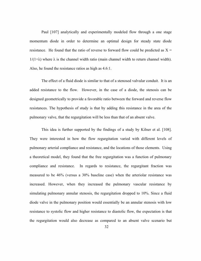
32
Paul [107] analytically and experimentally modeled flow through a one stage
momentum diode in order to determine an optimal design for steady state diode
resistance. He found that the ratio of reverse to forward flow could be predicted as X =
1/(1+λ) where λ is the channel width ratio (main channel width to return channel width).
Also, he found the resistance ratios as high as 4.6:1.
The effect of a fluid diode is similar to that of a stenosed valvular conduit. It is an
added resistance to the flow. However, in the case of a diode, the stenosis can be
designed geometrically to provide a favorable ratio between the forward and reverse flow
resistances. The hypothesis of study is that by adding this resistance in the area of the
pulmonary valve, that the regurgitation will be less than that of an absent valve.
This idea is further supported by the findings of a study by Kilner et al. [108].
They were interested in how the flow regurgitation varied with different levels of
pulmonary arterial compliance and resistance, and the locations of those elements. Using
a theoretical model, they found that the free regurgitation was a function of pulmonary
compliance and resistance. In regards to resistance, the regurgitant fraction was
measured to be 46% (versus a 30% baseline case) when the arteriolar resistance was
increased. However, when they increased the pulmonary vascular resistance by
simulating pulmonary annular stenosis, the regurgitation dropped to 10%. Since a fluid
diode valve in the pulmonary position would essentially be an annular stenosis with low
resistance to systolic flow and higher resistance to diastolic flow, the expectation is that
the regurgitation would also decrease as compared to an absent valve scenario but

33
without the penalty of high systolic pressure gradient corresponding to a high resistance
stenosis.
The premise of using a momentum diode valve was tested by Losaw [109]. He
studied two diode valve designs as pulmonary heart valve replacements. The first, a
nozzle valve, was a benchmark design. The geometry was designed using the long radius
nozzle design conventions as outlined in the ASME nozzle design manual, but with a
shorter profile [110]. The beta ratio, the ratio of the minor and major orifice diameters,
was 0.5. The second valve studied by Losaw was inspired by the Tesla diode. This diode
valve incorporated the curved channels similar to the valvular conduit.
The results of the diode valve were compared to that of SJM bileaflet, the nozzle
valve and absent valve case. He reported a regurgitation fraction of 15.8± 0.1% for a
cardiac output of 5.8 Lpm for the diode valve. This was roughly a 25% improvement
over the absent valve case of similar flow rate. The measured transvalvular gradient for
the diode valve was 4.2 ±0.6 mmHg, expectedly higher than that of the absent valve. Yet,
it is still reasonable. These findings support the idea that a momentum diode could serve
as a replacement pulmonary heart valve under certain conditions. Also, it suggests that
geometric changes may offer improved results.
Proposed Diode Design
The baseline design is based on the diode valve studied by Losaw [109]. The
valve has an elliptical contraction and a backchannel enclosed by an annular ring. The
34
cusp of the backchannel has an elliptical profile. The generally dimensioned cross-
section is shown in the figure below Figure 2.5.
α - impingement angle of backflow channel jet d – minor orifice diameter D – major orifice diameter β - ratio of minor to major orifice diameter, d/D L – overall length of the diode b – minor width of backflow channel B – Major width of backflow channel c – annular ring width
The concept is that during systole, flow will encounter little resistance from the
nozzle type entry. However, during diastole, retrograde flow would be impeded by the
smaller diameter and the flow from the backchannels reentering the central flow field and
Figure 2.5: Generically Dimensioned Diode Valve

35
angle. For the base design, the dimensions are as listed: impingement angle 60°, the β-
ratio is 0.5, L is 12.5mm, b is 1.2 mm and B is equal to 2.0 mm. The dimensional
variations of this design for other valves that were tested are shown in Table 2.1.
For the sake of manufacturing, a way to simplify the diode design was
investigated. The momentum diode valve has a contoured backchannel with an inner ring
to enclose it. A solid model rendering of the baseline design is shown in Figure 2.6a. A
much simpler design of the momentum diode valve was to eliminate the inner ring or, in
terms of the geometric parameters, let c = 0 (see Figure 2.6b). The open cusped valve
was then made in one piece without the need to machine and hold the inner ring in place.
All diodes were modeled using the 3D CAD software program SolidWorks. The
valves that were tested in vitro were made by a rapid prototyping machine with an
acrylonitrile-butadiene-styrene (ABS) plastic polymer. The valves for PIV testing were
replicas of the biological implant. They were made of 316L stainless steel and coated
with DLC pyrolitic carbon. The coating was a BioMedFlex® film coating had a thickness
of 0.1 - 4 µm, a coefficient of friction of 0.02 – 0.04, and a hardness of 12,000 N/mm2.

36
Table 2.1: Diode Design Dimensions
Parameter α β L b B c 1 (Baseline) 60 0.50 12.5 1.2 2.0
2 60 0.50 12.5 Inf Inf 0 3 75 0.50 12.5 1.2 2.0 4 75 0.50 12.5 Inf inf 0 5 90 0.50 12.5 1.2 2.0 6 90 0.50 12.5 Inf Inf 0 7 60 0.45 12.5 8 60 0.40 12.5
Figure 2.6: Solidworks Models of (a) a diode valve with an enclosed backchannel (backchannel diode); (b) diode valve with an open backchannel (open cusped diode)
37
CHAPTER THREE
RESEARCH METHODS
The primary objective of the present study is to test the hypothesis that a
motionless momentum diode valve can perform as a replacement pulmonary valve. The
review of the literature established that there is a particular need for a replacement valve
for patients born with congenital heart defects and suffer from pulmonary insufficiency.
Studies also show that the lower operating pressures of the right heart circulation allow
for less strict tolerances on pressure gradient and regurgitant fraction. The following
strategies will be implemented in order to further evaluate the hypothesis.
The first aim is to test the momentum diode valves in vitro over a range of
physiological conditions for transvalvular pressure gradients (TVG) and regurgitant
fractions (RF%) as functions of pulmonary impedance. They will be compared to
traditional replacement valves in the pulmonary position. The criteria for acceptable
performance is the ability to regulate flow to moderate and acceptable levels of RF% of
(0 - 20% is desired, less than 35% overall) and TVG (0-30 mmHg).
The second aim is to perform a parametric study using geometric variation of the
diode valve designs in order to determine how the geometry affects the valve
performance. Also, key design parameters that affect flow regulating performance will
be identified so that they can later be optimized.
38
Another objective is to evaluate the diode valve concept in vivo. An acute in vivo
test will be performed in the development of the surgical protocol and technique for the
implantation. It will also generate information on how to administer longer term tests.
Also, the experiment will produce preliminary information that may answer questions
such as: is the data similar to that in the in vitro setup? And how will the animal react to
the diode valve?
Finally, particle image velocimetry (PIV) will be used to study the hemodynamic
performance of different diode designs. Flow field data will be used to evaluate flow
patterns, the viscous and turbulent shear stress levels, and estimate the exposure times for
a particle (platelet). A threshold level of activation of 35 dynes-s/cm2 [54] will be used as
an upper benchmark for benign activation. The PIV data as a whole will help determine if
a momentum diode valve can meet the hemodynamic demands as a prosthetic heart
valve.
Mock Pulmonary Circulatory System
A mock circulatory system was used to assess the hemodynamic performance of
different diode designs in vitro. The system was based on many of the previous designs
discussed in the literature review. The mock pulmonary circulatory system (MPCS)
modeled the right heart circulation at various physiological settings. It contained open air
atrial chambers, ventricle chamber, a pulsatile pump, and compliance and resistance
elements. It allowed for pressure and flow measurements to be obtained as well as optical
39
flow measurements. Figure 3.1 shows a schematic of the MPCS used in the current
study.
The right atrium tank was a six (6) inch acrylic tube with one end closed off using
a delrin cap. This tank had an overflow connection so that the fluid height in the tank
remained constant.
The right ventricle assembly consisted of a balloon enclosed in a chamber. A
pneumatic cylinder was connected to the chamber with hosing. The cylinder action was
driven by a cam driven pump (Harvard 1423 Pulsatile pump). The amount of stroke that
the cylinder encounters was adjusted by changing the stroke volume on the Harvard
pump. This pump was designed so that the cycle rate (heart rate, HR) and systolic ratio
(SR%) are adjustable.
The test section was made of acrylic and houses the test valve (Figure 3.2). The
contraction was constructed to reduce the flow area from 62 mm diameter to 25 mm
diameter, the size of the prototype valves to be studied. The profile dimensions were
taken from a similar piece done by Figliola [111]. The distal section was modeled after
the human pulmonary artery. The internal artery dimensions (Figure 3.3) were scaled for
a 25 mm tissue annulus versus the 29 mm that was used by Philpot [79, 80]. The
passages were axisymmetric with respect to the flow centerlines.

40
The resistance and compliance needed to be adjustable in order to test at different
physiological states. The compliance in the system was modeled using two Windkessel
compliance chambers. They were PVC pipe 4” in diameter and 24” tall and one end is
capped. The chambers were positioned vertically, and there was a hose barb tee
connection in the end cap through which the blood analog flows. The top end of the
chambers were sealed with an inflatable rubber ball plugs so that the amount of trapped
air could be varied. This permitted for the adjustment of the tank compliance. The height
of the chambers and size of the test plugs allowed for the individual tank compliance to
be adjusted up to 4 mL/mmHg.
Figure 3.1: Schematic of the mock circulatory system used in this study. Arrows indicate flow direction. 1. Right atrium constant head tank; 2. Right ventricular
chamber; 3. Flow meter; 4. Test section 5; Mechanical heart valve; 6. Ball valves; 7. Capacitance chambers; 8. Holding tank; 9. Recirculating pump; 10. Pneumatic
cylinder; 11. Harvard Pulsatile pump; 12. Left atrium constant head tank

41
Figure 3.3: Pulmonary artery test section. Dimensions in mm.
Figure 3.2: Complete test section. RVP and PAP pressure taps shown.
42
In addition to the compliance, the pulmonary vascular resistance of the system
needed to be regulated. There was inherent resistance in the system resulting from the
tubing and connectors. There were also ball valves that could be used to regulate both the
resistance and the flow in each of the arterial branches. The ball valves were located
between compliance chambers and the second open air tank that acted as the left atrium.
The left atrium tank was designed just like the right atrium tank. It was also used to
change the resistance.
Global Flow and Pressure Measurements
The global tests were conducted as a mean of characterizing the hydrodynamic
performance of the different valve designs. All data was acquired using an automated
data acquisition (DAQ) system controlled by NI Labview®.
Instantaneous and mean flow data were measured using a Carolina Medical®
model 501 electromagnetic flowmeter. One probe was attached as shown in Figure 3.1.
An additional probe was used to measure flow in one of the pulmonary artery branches.
The instantaneous flow readings were separated into forward and reverse flow data by a
zero crossing algorithm. Numerical integration was performed on all the flow data to
yield the net flow rate through the valve as well as the positive (Qforward) and negative
flow rates (Qreverse) components. Equation 1 shows the simple integration technique used
to determine mean flow.
∆
∑ · (1)
43
The regurgitation fraction was calculated using this data with the following
equation:
% · 100 (2)
The pressure transducers were BD physiological pressure transducers. The
pressure taps were located so that the right ventricular pressure (RVP) and the pulmonary
artery pressure (PAP) were measured (Figure 3.2). The transducers were located on a
holder fixed to the floor to minimize transmission of system vibrations.
With this information, the transvalvular pressure gradient (TVG), mean
pulmonary artery pressure (mPa), pulmonic impedance (PVZ) and pulmonic vascular
resistance (PVR), compliance and effective orifice area (EOA) were calculated. Mean
pulmonary artery pressure was calculated the same way that the mean flow rate was
found. The pressure gradient across the valve was found using equation 3.
(3)
System resistance and compliance were calculated in two manners. To measure
the system impedance, a procedure carried out by Gohean, et al. [112] was followed.
Fourier analysis was used to transform the time-based signals into frequency domain to
obtain a spectrum for both PAP and flow rate (Q) [9, 113-116].
| || | (4)

44
The impedance at the zeroth harmonic (Z0) is otherwise known as the pulmonary
vascular resistance (PVR). Pulmonary vascular compliance can also be extracted from
the spectrum data as the first harmonic, Z1, is shown to be inversely proportional to the
system compliance [9].
The second method of calculating PVR and compliance was to use their
respective definitions. These approximations are used during data acquisition as a means
to estimate the resistance and compliance during system tuning.
/ (6)
·· 1000 (7)
The effective orifice area (EOA) is an index of how well the valve uses its
primary orifice area and is another way of gauging how much a valve obstructs flow. It
was defined by the following equation for saline [117]:
. ∆EOA (8)
Optical Flow Field Measurements
In addition to global flow data, optical flow field data was collected using PIV.
The flow field velocity maps assessed for the thrombogenetic potential of each valve by
magnitude of stress, stress exposure times, and areas of stasis.
45
Particle Image Velocimetry
Particle image velocimetry (PIV) is a noninvasive method of measuring velocity.
It provides and indirect fluid flow measurement and also allows for whole flow fields to
be captured. Typically, an experimental setup of a PIV system has several subsystems.
Tracer particles are added to the flow. They are illuminated in a plane by a light sheet by
means of a laser. This happens at least twice within a short, known time interval and the
light scattered by the particles is recorded with a high quality lens of two separate frames
on a cross correlation CCD sensor. The images are stored directly on a computer and are
evaluated in order to determine the displacement of the particle images. This is done by
dividing the PIV recordings into small sub-areas called “interrogation areas”. For each
interrogation area, the displacement vector for the particles is found by means of auto and
cross-correlation methods [118].
There are some considerations that need to be taken into account when setting up
the PIV system. One issue is that of velocity lag and therefore particle size. Tracer
particles should follow the motion of the fluid elements. Small particles will follow flow
better. Light source power is another area to consider. While high gas flows may require
a high power light source in order to get light scatter off of small tracer particles, liquid
flows can tolerate larger particles. These scatter more light; therefore, a lower peak power
laser can be used. The duration of the illumination pulse should be short enough to
‘freeze’ the particle motion; thus, no streaks or blurry images. The time delay between
pulses should be long enough for the particles to have detectable displacement, but short
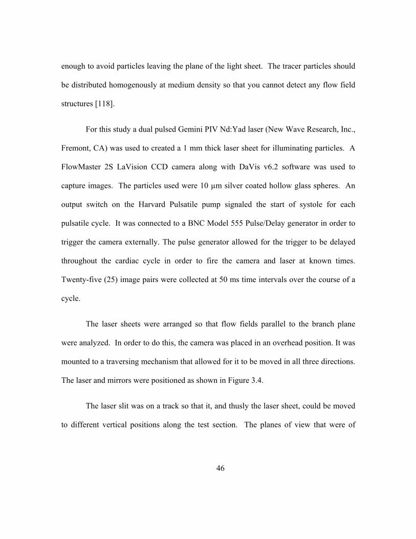
46
enough to avoid particles leaving the plane of the light sheet. The tracer particles should
be distributed homogenously at medium density so that you cannot detect any flow field
structures [118].
For this study a dual pulsed Gemini PIV Nd:Yad laser (New Wave Research, Inc.,
Fremont, CA) was used to created a 1 mm thick laser sheet for illuminating particles. A
FlowMaster 2S LaVision CCD camera along with DaVis v6.2 software was used to
capture images. The particles used were 10 µm silver coated hollow glass spheres. An
output switch on the Harvard Pulsatile pump signaled the start of systole for each
pulsatile cycle. It was connected to a BNC Model 555 Pulse/Delay generator in order to
trigger the camera externally. The pulse generator allowed for the trigger to be delayed
throughout the cardiac cycle in order to fire the camera and laser at known times.
Twenty-five (25) image pairs were collected at 50 ms time intervals over the course of a
cycle.
The laser sheets were arranged so that flow fields parallel to the branch plane
were analyzed. In order to do this, the camera was placed in an overhead position. It was
mounted to a traversing mechanism that allowed for it to be moved in all three directions.
The laser and mirrors were positioned as shown in Figure 3.4.
The laser slit was on a track so that it, and thusly the laser sheet, could be moved
to different vertical positions along the test section. The planes of view that were of
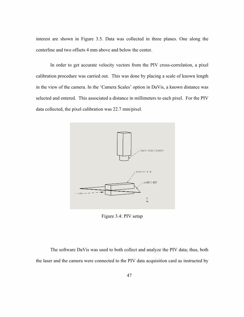
47
interest are shown in Figure 3.5. Data was collected in three planes. One along the
centerline and two offsets 4 mm above and below the center.
In order to get accurate velocity vectors from the PIV cross-correlation, a pixel
calibration procedure was carried out. This was done by placing a scale of known length
in the view of the camera. In the ‘Camera Scales’ option in DaVis, a known distance was
selected and entered. This associated a distance in millimeters to each pixel. For the PIV
data collected, the pixel calibration was 22.7 mm/pixel.
The software DaVis was used to both collect and analyze the PIV data; thus, both
the laser and the camera were connected to the PIV data acquisition card as instructed by
Figure 3.4: PIV setup
48
the DaVis catalog. The laser and camera triggering were operated by the software.
However, the timing needed to be externally controlled so that images could be acquired
at a known point in the cardiac cycle. A switch output from the Harvard pulsatile pump
was connected to the pulse generator as a trigger. The pulse generator accepted this
trigger and then output a TTL signal to the DaVis card. This output could be delayed
from the initial trigger by any time. In this case, the delays were from 0 – 750 ms in 50
ms increments.
The images were captured and stored using the ’Sequence’ command. At each
time step, twenty-five images were collected. The files were named so that it identified
Figure 3.5: Flow Field Planes that will be analyzed with PIV

49
the time step, the plane of view and the PVR level to which the system is tuned.
The ‘Image Processing’ command was used to batch process the 25 image pairs. Each
image pair was analyzed using a double pass cross-correlation scheme with an initial
interrogation window of 64x64 pixels and a final interrogation window of 32x32 pixels.
The second pass was offset. A peak velocity filter of 2 – 4 m/s was employed based on
expected maximum velocities. A mask file was created to block the regions of the images
that were not within the flow field. An ensemble average of these images was found
using the algorithm in DaVis. Each individual (from each image pair) and mean file was
saved as a text file with the results from DaVis cross-correlation. The text files included
the x and y positions, u, the velocity in the x direction and v, the velocity in the y
direction. The mean data files contained the same data with the mean velocity
components, instead of the instantaneous velocities. The variable n represents
the number of cycles.
∑ (9)
∑ (10)
This data was then further analyzed using in house algorithm written in Matlab.
The viscous shear stresses were calculated using shearing strain rate based on the time-
averaged flow velocities, , , of twenty five cycles as described in equation 11. The
number of image pairs, N, was chose based on the convergence of urms as N was
increased. The values for urms and N are shown in
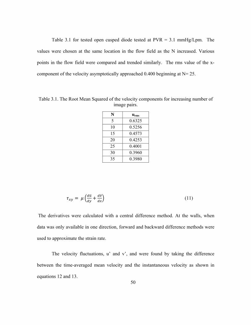
50
Table 3.1 for tested open cusped diode tested at PVR = 3.1 mmHg/Lpm. The
values were chosen at the same location in the flow field as the N increased. Various
points in the flow field were compared and trended similarly. The rms value of the x-
component of the velocity asymptotically approached 0.400 beginning at N= 25.
Table 3.1. The Root Mean Squared of the velocity components for increasing number of image pairs.
N urms 5 0.6325 10 0.5256 15 0.4573 20 0.4253 25 0.4001 30 0.3960 35 0.3980
(11)
The derivatives were calculated with a central difference method. At the walls, when
data was only available in one direction, forward and backward difference methods were
used to approximate the strain rate.
The velocity fluctuations, u’ and v’, and were found by taking the difference
between the time-averaged mean velocity and the instantaneous velocity as shown in
equations 12 and 13.
51
(12)
(13)
The Reynolds shear and normal stresses were found with equations 14 -16. For each
cycle, the product of the velocity fluctuations was found. These products were then
averaged in order to yield the turbulent shear stress as showing in equation 14. The
turbulent normal stresses were found in a similar manner.
(14)
(15)
(16)
Finally, the turbulence intensities were found with the following expressions:
∑ (17)
∑ (18)
All stress values are reported with units of dynes/cm2.
Laser Doppler Velocimetry Measurements
Laser Doppler velocimetry (LDV) is a method used to measure velocities at a
point. It is best used to characterize local turbulent properties as a result of its high

52
temporal and spatial resolution. The LDV system used here was a TSI® computer-
controlled, two-component fiber optic system with dual Bragg-cells, digital spectral flow
analyzer, and a multiband 6W Spectra-physics Stabilite argon-ion laser source. The laser
head was placed on a traversing mechanism that moved in the x, y and z directions so that
the beam could be positioned anywhere in the flow. The system provided two-
dimensional velocity component information with both forward and reverse flow
measuring capability. The LDV setup is shown in Figure 3.6. LDV measurements were
collected in the areas of elevated Reynolds shear stresses that were identified by the PIV
measurements and the power spectrums were calculated.
The data was initially sorted by grid location. Then, the 12,000 points were
divided into different cycles. Any cycles containing more than 900 data points were
omitted. This was to maintain Zeros were appended to any cycles with less than 900
points so that each cycle had an equal same number of cycles. The data was then written
out into a column of data for each cycle. So, instead of a column array of 12000 points,
there were 12 columns of approximately 890 points.

53
A second analysis sorted data from the initial program and calculated the average
over the cycle. A quasi steady condition was assumed for the pulsatile cycle over 10 data
points. Therefore, the cycles were divided into 89 periods of 10 points each and the
average values for these over all the cycles were determined. The velocity fluctuations,
u’ and v’, were found for each point in the cycle by subtracting the mean value from the
velocity component.
In the final phase of the analysis, the fast Fourier Transform (FFT) was performed
on the data. The FFT was done on the autocorrelation of the both the axial and radial
velocity components. Then, the ensemble average was calculated. The order of the
operations was changed (ensemble average, then FFT) without any differing effect. A
100 point discrete Fourier transform (DFT) is designated. The magnitude of each
Figure 3.6: LDV setup
54
complex value was found, and the frequency was normalized from 0 - 500 Hz. A basic
moving average smoothing function with a window size of 3-5 points was applied to the
final magnitude curves.
Test Fluids
The blood analog solution for global testing and measurements was a 40% by
volume glycerin/water solution. Sodium chloride was added in order to provide a charge
for the electromagnetic flow meter. The kinematic viscosity was checked using a
Cannon-Fiske U-tube viscometer and the specific gravity with a hydrometer. The
solution typically had a viscosity of 3.25 cSt and a specific gravity of 1.095. For optical
studies, the refractive index of the blood analog needed to match that of the acrylic test
section in order to minimize distortion. Therefore, a solution of 79% saturated sodium
iodide, 20% glycerin and 1% water. The resulting solution had a refractive index ranging
from 1.46 - 1.49, a kinematic viscosity similar to that previously stated, and specific
gravity of 1.6. Both solutions were mixed by using a scale to measure out the appropriate
percentage of components and mixed thoroughly. Since kinematic similitude was held,
the Reynolds number for all the testing with glycerin/water solution as well as the
glycerin/water/sodium iodide solution was the same. For all tests, Re was on average
1407 for flow rates of 5 Lpm with maximum values reaching 7037 for flow rates of 25
Lpm.
55
CHAPTER FOUR
DIODE PERFORMANCE TESTING RESULTS
Preliminary Testing
The first two criteria that the diode valves must meet in order to be considered for
a pulmonary valve replacement are regulating flow so that the regurgitant flow less than
35% and the transvalvular gradient is less than 25 mm Hg. As a preliminary study, the
performance of the diode valves were compared to that of the mechanical heart valves
commonly used as pulmonary heart valves. The mock pulmonary circulatory system was
used to test all the valves.
MPCS Variations
The ventricle in the preliminary tests was driven by compressed air regulated with
a system of pneumatic solenoid valves instead of the Harvard pulsatile pump. The valve
timing was controlled using a BNC pulse generator. The stroke volume of the ventricle
was maintained by adjusting a needle flow control valve on the inlet hose that lead to the
ventricle chamber. Also, an alternate style of compliance chambers was used during
these tests. These chambers consisted of a rubber hose housed in a 4” diameter acrylic
tube. The chamber could be pressurized using a pressure bulb and vented in order to
adjust the resistance and compliance of the system. The pressure transducers used were
Druck LPM 5480 in lieu of the BD physiological transducers.

56
Test Conditions
For these tests, the following conditions were maintained: cardiac output of 5
Lpm, pulse rate of 75 beats per minute (bpm), and a systolic ratio of 45%. The PVR was
then varied between 1 and 5 mm Hg/Lpm. This was done by changing the downstream
resistance by adjusting the ball valves, the height of the left atrial tank, and the stroke
volume of the pump. The system compliance is coupled with the system resistance and
was held between 2 ml/ mm Hg and 6 ml/mm Hg for these set of tests.
The baseline diode valve design was tested alongside a St. Jude Mechanical
bileaflet valve (SJMBV) and the MedicalCV Omnicarbon tilting disk valve (OTD). Each
valve was tested in the MPCS over a range pulmonary vascular resistance. These results
have been previously reported in Camp et al. [119].
Diode to Mechanical Heart Valve Comparison
Pressure and Flow Curves
The right ventricular pressure, pulmonary artery pressure and flow rate signals
were obtained for each type of valve. Figure 4.1 and Figure 4.2 are the traces for the
SJMBV and OTD valve. In general, the pressure and flow signals are consistent with
physiological traces [12]. The PAP curve for each displays a clear dicrotic notch at the
point of valve closure. At this point, the flow rate in both cases shows some valve
regurgitation or retrograde flow. The flow rate curve oscillates a little around the zero,
indicating leakage through the valves. The RF% for both the OTD valve and the SJMBV
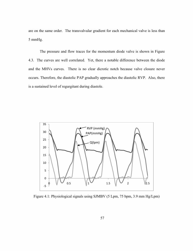
57
are on the same order. The transvalvular gradient for each mechanical valve is less than
5 mmHg.
The pressure and flow traces for the momentum diode valve is shown in Figure
4.3. The curves are well correlated. Yet, there a notable difference between the diode
and the MHVs curves. There is no clear dicrotic notch because valve closure never
occurs. Therefore, the diastolic PAP gradually approaches the diastolic RVP. Also, there
is a sustained level of regurgitant during diastole.
Figure 4.1: Physiological signals using SJMBV (5 Lpm, 75 bpm, 3.9 mm Hg/Lpm)
‐5
0
5
10
15
20
25
30
35
0 0.5 1 1.5 2 2.5
RVP (mmHg)PAP(mmHg)
Q(lpm)
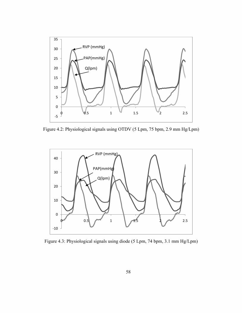
58
Figure 4.3: Physiological signals using diode (5 Lpm, 74 bpm, 3.1 mm Hg/Lpm)
‐10
0
10
20
30
40
0 0.5 1 1.5 2 2.5
RVP (mmHg)
PAP(mmHg)
Q(lpm)
Figure 4.2: Physiological signals using OTDV (5 Lpm, 75 bpm, 2.9 mm Hg/Lpm)
‐5
0
5
10
15
20
25
30
35
0 0.5 1 1.5 2 2.5
RVP (mmHg)
PAP(mmHg)
Q(lpm)

59
Performance Data
Each valve was tested at different levels of PVR. The regurgitant fraction and
pressure gradient were calculated for each case using equations 2 and 3. The effective
orifice area was also found (Equation 8). Figure 4.4 summarizes all the RF% and TVG
data. The EOA calculations are listed in Table 4.1.
Table 4.1: Summary of effective orifice area (5 Lpm and 75 bpm)
Cardiac Output (Lpm)
PVR (mm Hg/Lpm)
EOA (cm2)
SJMBV 5.1± 0.1 3.05 ± 0.1 3.64 OTD Valve 5.2 ± 0.1 2.9 ± 0.1 2.45
Diode 5.1 ± 0.1 3.0 ± 0.1 1.24 Nozzle 5.1 ± 0.2 3.0 ± 0.1 1.13
Figure 4.4: Regurgitant Fraction (RF) and peak to peak transvalvular gradient at 5 Lpm
0
5
10
15
20
25
30
0 1 2 3 4 5
0
2
4
6
8
10
12
14
16
18
20
RF%
PVR (mmHg/Lpm)TV
G (m
mHg)
SJM ‐ TVG
Diode ‐ TVG
Nozzle ‐ TVG
Series8
SJMBV ‐ RF%
Diode ‐ RF%
Nozzle ‐ RF%
OTDV RF%
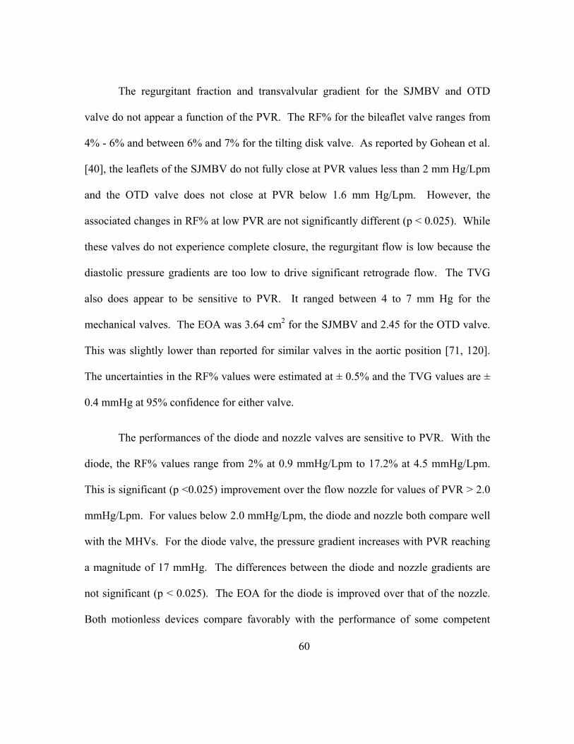
60
The regurgitant fraction and transvalvular gradient for the SJMBV and OTD
valve do not appear a function of the PVR. The RF% for the bileaflet valve ranges from
4% - 6% and between 6% and 7% for the tilting disk valve. As reported by Gohean et al.
[40], the leaflets of the SJMBV do not fully close at PVR values less than 2 mm Hg/Lpm
and the OTD valve does not close at PVR below 1.6 mm Hg/Lpm. However, the
associated changes in RF% at low PVR are not significantly different (p < 0.025). While
these valves do not experience complete closure, the regurgitant flow is low because the
diastolic pressure gradients are too low to drive significant retrograde flow. The TVG
also does appear to be sensitive to PVR. It ranged between 4 to 7 mm Hg for the
mechanical valves. The EOA was 3.64 cm2 for the SJMBV and 2.45 for the OTD valve.
This was slightly lower than reported for similar valves in the aortic position [71, 120].
The uncertainties in the RF% values were estimated at ± 0.5% and the TVG values are ±
0.4 mmHg at 95% confidence for either valve.
The performances of the diode and nozzle valves are sensitive to PVR. With the
diode, the RF% values range from 2% at 0.9 mmHg/Lpm to 17.2% at 4.5 mmHg/Lpm.
This is significant (p <0.025) improvement over the flow nozzle for values of PVR > 2.0
mmHg/Lpm. For values below 2.0 mmHg/Lpm, the diode and nozzle both compare well
with the MHVs. For the diode valve, the pressure gradient increases with PVR reaching
a magnitude of 17 mmHg. The differences between the diode and nozzle gradients are
not significant (p < 0.025). The EOA for the diode is improved over that of the nozzle.
Both motionless devices compare favorably with the performance of some competent

61
mechanical and bioprosthetic valve in the aortic position [71, 120]. Uncertainties in the
RF% values were estimated at ±1.2% and TVG values at ±0.7 mmHg at 95% confidence
for the motionless devices.
Despite the identical central flow areas of both the diode valve and the nozzle,
the diode valve showed more forward flow and less regurgitant flow than the nozzle for a
given setting of the MPCS. The implication is that regurgitant flow can be reduced by
diode design, such as by use of the backchannel diode. The diode design increases
resistance to backflow. The enhanced forward flow is likely due to forward flow
expanding into the channels over slightly less resistance in the forward direction.
Summary
The results of this study continue to support the idea that a motionless momentum
diode valve can be used to regulate flow in the pulmonary position. The diode valve
showed improvement in ability over the flow nozzle to impede regurgitant flow. For a
PVR range of 1 to 5 mmHg/Lpm, the diode valve yielded a RF% of 2% to 17% as
compared to the 2% to 23% for the nozzle. Both valves had TVG values up to 17 mmHg.
62
CHAPTER FIVE
ANIMAL MODEL RESULTS
Introduction
In this portion of the study, the fluid diode valve was tested in a swine model in
order to compare the pressure gradients and regurgitant fractions. The objectives of the
acute non-survival animal model were to develop implantation and surgical strategies, to
assess the immediate tolerance and eliminate catastrophic response to diode implantation,
and to obtain in vivo physiological data to validate in vitro test results.
Methods
In vitro system setup
Valve tests were conducted in the mock circulatory system (MCS) as described in
chapter 3. For these tests, conditions were maintained at a nominal cardiac output of 5
Lpm at a pulse rate of 110 bpm and systolic ratio of 40% [5] for comparison with the in
vivo studies. The pulmonary vascular resistance was varied between 1 to 4.5 mm
Hg/Lpm. This change was done by adjusting the downstream resistance to increase the
mean pulmonary artery pressure while maintaining flow rate and pulse rate.
Valve designs
The diode valve design studied was an open cusped diode with a 60˚ impingement
angle (design 2 in Table 2.1). The diode has groves on the outer diameter that act as
suture rings. These can be seen in Figure 2.6. The biological implant was constructed of
63
316L stainless steel and was coated with a carbon thin film coating. The BioMedFlex®
film coating is a proven coating that has been used in medical blood flow devices
requiring a nonthrombogenic surface.
Animals and operative procedures
Structural integrity, anti-thrombogenicity/anti-calcification, implantation
techniques, and hemodynamic performance of the diode in a biological milieu were
tested. A 70 kg farm swine was adopted due to similarities to humans in the coagulation
cascade, platelet function, and platelet-leuckocyte-enthothelial cell interaction. These
make pig models more suitable for analyzing thrombosis and platelet activation resulting
from prosthetic valves [121]. Following general endotracheal anesthesia, a full median
sternotomy was performed, and the heart suspended in a pericardial well.
Cardiopulmonary bypass cannulas were placed into the ascending aorta, and directly into
both superior and inferior vena cavae. After systemic heparin anticoagulation was
achieved, as demonstrated by an activated clotting time > 400 seconds, the animal was
placed on complete cardiopulmonary bypass. The main pulmonary artery was opened,
and the native pulmonary valve excised.
A test valve was pre-implanted in a Gore-Tex vascular graft. This graft was then
sutured into the pulmonary artery. The patient was weaned off by-pass. Pressure
catheters were implanted and a flow probe placed around the PA. Data were recorded
for up to two hours. Following euthanasia, the valve was retrieved and analyzed for
platelet deposition and the lungs and heart examined.
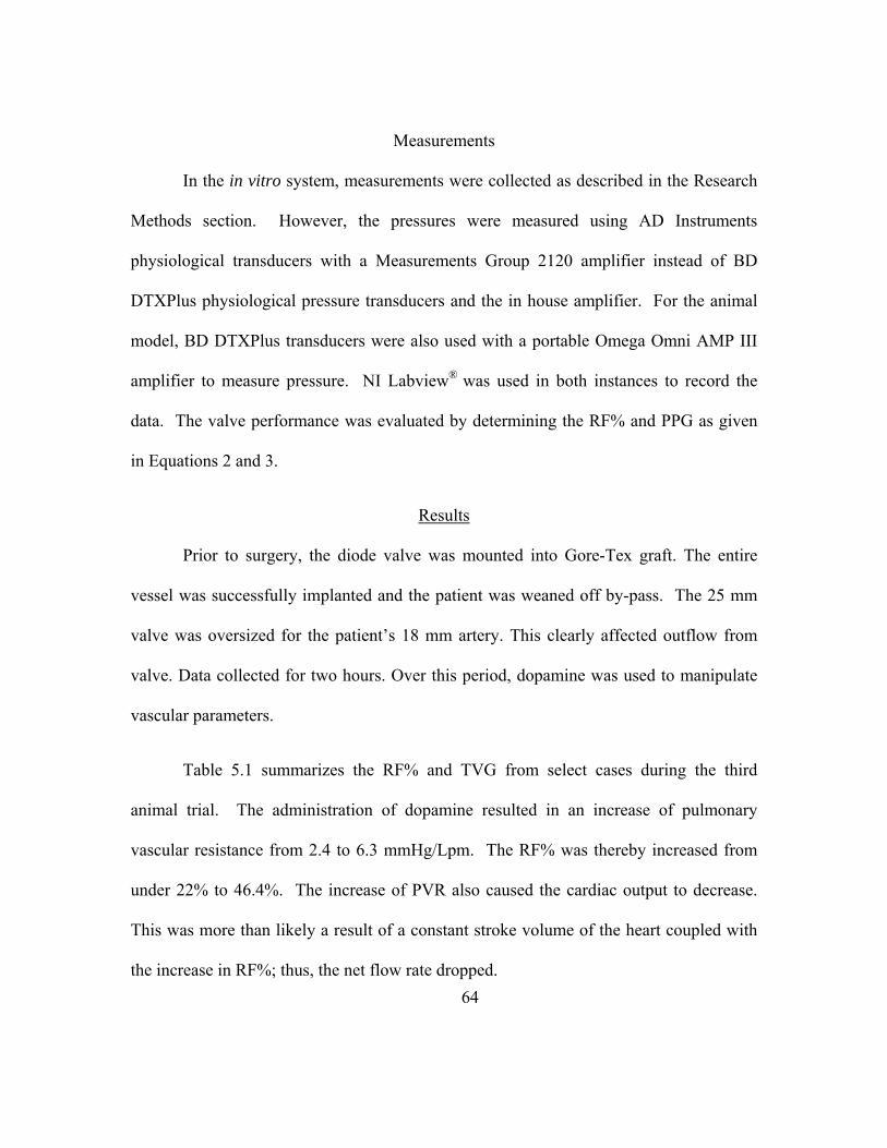
64
Measurements
In the in vitro system, measurements were collected as described in the Research
Methods section. However, the pressures were measured using AD Instruments
physiological transducers with a Measurements Group 2120 amplifier instead of BD
DTXPlus physiological pressure transducers and the in house amplifier. For the animal
model, BD DTXPlus transducers were also used with a portable Omega Omni AMP III
amplifier to measure pressure. NI Labview® was used in both instances to record the
data. The valve performance was evaluated by determining the RF% and PPG as given
in Equations 2 and 3.
Results
Prior to surgery, the diode valve was mounted into Gore-Tex graft. The entire
vessel was successfully implanted and the patient was weaned off by-pass. The 25 mm
valve was oversized for the patient’s 18 mm artery. This clearly affected outflow from
valve. Data collected for two hours. Over this period, dopamine was used to manipulate
vascular parameters.
Table 5.1 summarizes the RF% and TVG from select cases during the third
animal trial. The administration of dopamine resulted in an increase of pulmonary
vascular resistance from 2.4 to 6.3 mmHg/Lpm. The RF% was thereby increased from
under 22% to 46.4%. The increase of PVR also caused the cardiac output to decrease.
This was more than likely a result of a constant stroke volume of the heart coupled with
the increase in RF%; thus, the net flow rate dropped.
65
Table 5.1. Select Results from the Animal Model Testing with 95% Confidence Intervals
HR (bpm)
CO (Lpm)
PVR(mmHg/Lpm)
Compliance(ml/mmHg)
RF% TVG (mmHg)
158 6.2 ± 0.07 2.1 ± 0.04 2.2 ± 0.08 11.3 ± 0.70 10.9 ± 2.86161 6.2 ± 0.17 2.4 ± 0.07 2.3 ± 0.20 15.1 ± 1.35 13.9 ± 2.55130 4.6 ± 0.15 2.4 ± 0.09 3.1 ± 0.1 21.9 ± 1.4 21.2 ± 3.18123 2.7 ± 0.31 6.3 ± 0.08 1.0 ± 0.1 46.4 ± 6.09 22.7 ± 4.08
A representative flow and pressure curve from the animal study is shown in
Figure 5.1. The curve generated by the MPCS is comparable to figure shown. There is a
diastolic pressure gradient of about 10 mmHg. The PVR was 4.4 mmHg/Lpm, a PVC of
2.2 mL/mmHg, and the flow ranged from 15 Lpm to - 8 Lpm giving way for a RF% of
29%.
The resulting regurgitant fractions and transvalvular gradient as a function of
PVR for both the in vitro and in vivo studies are shown in Figure 5.2 and Figure 5.3. The
RF% for the in vivo tests levels off around 30% for high values of PVR. The in vitro
curve shows a similar trend. The RF% is held to moderate levels of less than 30% for
resistances below 3 mmHg/Lpm.
The pressure gradients are higher for the animal models than those measured in
the mock circulatory system. The differences are more noticeable at resistances above 2
mmHg/Lpm. This variance may be a result of the change in compliance noted at each
these points. Also, the locations of the pressure catheters could not be replicated in the
animal model and this could affect the pressure measurements.

66
In both models, there is relationship between the pulmonary vascular resistance
and pulmonary vascular compliance. The PVC is shown to decrease as PVR increased.
The curves for both systems are shown in Figure 5.4. Separation is seen at PVR values
below 2.5 mmHg/Lpm.
Summary
The acute animal model demonstrated no catastrophic effects of using a
motionless pulmonary valve. The patient was weaned successfully off by-pass. Valuable
lessons regarding pharmacology were learned. An implantation strategy was developed
that can be carried into a chronic test animal model. In vivo performance results are
consistent in both tendency and magnitude with in vitro findings. Under normal values of
compliance (2 to 3 mL/mmHg) and pulmonary vascular resistance (2.3 to 3 mmHg/Lpm),
Figure 5.1. Example flow and pressure curve collected during animal tests using a 25 mm opencusped diode valve
‐10
0
10
20
30
40
0 0.5 1 1.5 2 2.5
RVP (mmHg)
PAP(mmHg)Q(lpm)

67
regurgitant fraction and transvalvular gradients remain within levels known to be well
tolerated in humans. Under the influence of dopamine, the vascular resistance was
increased to over 6 mmHg/Lpm and compliance decreased to 1 mL/mmHg, resulting in
increased levels of regurgitant fraction and higher gradients. However, a compromising
factor in these tests was a valve size to patient mismatch, which likely altered valve flow
into the pulmonary artery.
Figure 5.2. PVR vs RF% for both the in vivo and in vitro tests. In vitro test completed at 110 bpm, CO = 5 Lpm.
‐5
0
5
10
15
20
25
30
35
40
1 2 3 4 5
RF%
PVR (mmHg/Lpm)
In Vivo Results
In Vitro Results

68
Figure 5.4. PVR vs PVC for animal model and the in vitro model with a 25 mm open cusped diode valve.
0
0.5
1
1.5
2
2.5
3
3.5
0 1 2 3 4 5 6 7
PVC (m
L/mmHg)
PVR (mmHg/Lpm)
PVC ‐ in vivo
Figure 5.3. TVG vs RF% for both the in vivo and in vitro tests. In vitro test completed at 110 bpm, CO = 5 Lpm.
0
5
10
15
20
25
30
35
40
0 1 2 3 4 5 6 7
TVG (m
mHg)
PVR (mmHg/Lpm)
in vivo Results
in vitro Results

69
CHAPTER SIX
PARAMETRIC STUDY RESULTS
There were two sets of comparison tests. The first study compared the baseline
diode design to designs 2 - 6 that had varying impingement angles and inner ring
configurations (Table 2.1). The second set of tests compared three valves with different
beta ratios (inner orifice diameters). The designs, 1, 7 and 8, are also listed in Table 2.1.
.
Test conditions
All the diode valves were tested in vitro in the MPCS as described in Chapter 3.
The system was tuned so that the pulmonary vascular resistance was varied between 1.5
and 6.5 mmHg/Lpm. For the first tests, the cardiac output was maintained at 5 Lpm. For
the beta ratio test, the cardiac output was maintained at 4 Lpm. This decrease in flow rate
was necessary to ensure that a maintaining a constant flow rate would be achievable over
a range of PVR levels. The heart rate for all tests was held at 75 bpm.
The operating values of pulmonary vascular resistance and compliance reported
are determined based on the spectral method of Gohean et al. (2005) using the
instantaneous flow rate and pressure signals, but nominal values were set based on
observed pressure and flow traces. A characteristic compliance – resistance curve of the
system is given in Figure 6.1 for a system containing a 25 mm open cusp diode valve
using blood analog. The system is adjustable over the range of pulmonary vascular

70
resistance (PVR) of 0.5 to 6 woods and a pulmonary vascular compliance of between 6 to
1 mL/mm Hg. The PVR was changed in this work by increasing flow resistance
downstream of the Windkessel compliances.
Results – Varying α and Inner Ring
The six diodes with different impingement angles and cusp designs were tested at
similar pulmonary vascular resistances. The goals of PVR = 2.5, 3.5, 4.5 and 5.5
mmHg/Lpm were targeted. The resulting PVR varied as did the cardiac output. For each
setting, data was sampled for 120 seconds (150 cycles). Three replications of each data
point were recorded. The cardiac output and PVR was averaged for the three points and
Figure 6.1. Characteristic Resistance - Compliance Curve for an Open Cusped Diode Valve
0
1
2
3
4
5
6
0 2 4 6 8
PVC (m
l/mmHg)
PVR (mmHg/Lpm)

71
the 95% confidence interval was calculated for each. The overall cardiac output for all
tests was 5.05 ± 0.3 Lpm. The resulting regurgitant fractions and transvalvular gradients
were also averaged and reported with their 95% confidence intervals.
Figure 6.2 shows the both the RF% and pressure gradient as a function of PVR for
each backchannel diode. This illustrates any influence that the impingement angle may
have on the performance for the backchannel valve. The pressure gradient increases with
increasing PVR for all the valves shown. This is expected as the increase in upstream
pressure must increase to drive the flow needed to maintain a constant cardiac output.
The overall TVG values range from 9.38 ± 0.05 to 22.5 ± 0.318 mmHg. Since the PVRs
are not exactly the same for each valve, point to point comparisons are not truly valid.
The results do imply that the differences between the TVG curves are not significant (p-
value < 0.025). No valve shows more than a 10% improvement over another. The
impingement angle was not expected to have a great influence on the pressure gradient.
The regurgitant fraction data points in Figure 6.2 also show that the RF% to be a
function of PVR. There is some separation between the curves in these results. At the
PVR levels between 2.4 and 2.6 mmHg, the backchannel diode with a 60˚ has a RF% that
is significantly lower RF% than the other valves with a 21% difference. As PVR was
increases, the improvement decreases. The valve with 75˚ impingement angle seems to
have a lower RF% than that with a 90˚ angle at lower resistances.

72
The open cusped diode valves are compared in Figure 6.3. The difference
between the behaviors of these valves is more pronounced than with the backchannel
diodes. The transvalvular gradient for the 60˚ open cusped valve is 30-35% higher than
that of the other two valves at some points. As PVR increases, the pressure gradient curve
for the 60˚ valve becomes less sensitive to PVR. The pressure gradients range from 16.7
to 27.4 mmHg for PVRs between 2.6 to 5.3 mmHg/Lpm. The 75˚ valve has the lowest
TVG for all resistances of the three valves for point at PVR less than 5.5mmHg/Lpm with
differences between the 75˚ and 90˚ being as high as 13%.
The RF% for all open cusped diode valves for a range of PVR is also shown in
Figure 6.3. Overall, the order of the regurgitant fraction curves follows that of the
pressure gradients. For resistance levels higher than 3.5 mmHg/Lpm, the 75˚ valve has
the lower RF%, the 90˚ valve is in the middle, and the 60˚ has the highest. The
regurgitant fraction percentages for the 60˚ valve were measured between 18 and 40%.
At the endpoints the uncertainties make it such that the difference between the valve
regurgitant fractions is not significant.

73
Figure 6.3: PVR vs RF% and TVG (mmHg) for all open cupsed diode valves (β=0.50) with 95% confidence intervals
0
5
10
15
20
25
30
35
40
45
2 3 4 5 6 7
RF% & TVG (m
mHg)
PVR (mmHg/Lpm)
TVG ‐ OC60TVG ‐ OC90TVG ‐ OC75RF% ‐ OC60RF% ‐ OC75RF% ‐ OC90
Figure 6.2: PVR vs RF% and TVG (mmHg) for all backchannel diode valves (β=0.50) with 95% confidence intervals
0
5
10
15
20
25
30
35
40
45
2 3 4 5 6 7
RF% & TVG (m
mHg)
PVR (mmHg/Lpm)
TVG ‐ BC60TVG ‐ BC75TVG ‐ BC90RF% ‐ BC60RF% ‐ BC75RF% ‐ BC90
74
Figure 6.4, Figure 6.5 and Figure 6.6 compare the effect of cusp design on the
pressure gradient and RF%. Figure 6.4 shows the RF% and TVG versus PVR for the
open cusped and backchannel diodes with 60˚ impingement angles. At the lowest
resistance, the difference in the gradients is not significant. As the PVR increases, the
open cusped diode experiences significantly higher pressure gradients than that of the
backchannel diode. The open cusped diode has transvalvular gradients between 50-78%
higher than that of the backchannel diodes. The behavior of the RF% for these valves
again coincides with that of the TVG. The open cusped diode at pulmonary vascular
resistances above 3 mmHg/Lpm has regurgitant flow up to 10% higher than the
backchannel diode.
The performance of the backchannel and open cusp diode with 75˚ angles as a
function of PVR is shown in Figure 6.5. There is no significant difference in the pressure
gradients for either valve over the range of resistances. There is also no significant
difference between the RF% values. This is contrary to the valves with α = 60˚.
The two cusp designs when coupled with an impingement angle of 90˚ are
compared in Figure 6.6. The transvalvular gradient curves are separated by a discernible
difference. The open cusped diode has a slightly higher TVG than the backchannel
diode. The pressure gradients are approximately 12 - 15% higher for the open cusped
valve. However, the cusp design has no noticeable effect on the RF% for valves with
90˚.

75
In summary, for both the backchannel and open cusped diode designs, there
appears to be a relationship between the valve performance and the impingement angle.
The 60˚ backchannel diode has the lowest RF% and TVG for some levels of the
resistance among the backchannel valves. Conversely, the 60˚ open cusped valve has
markedly higher RF% and TVG measurements versus the other two valves. The valve
with the 75˚ angle is the best performing open cusped design. Also, the results of this
study show the effect of the impingement angle seems less influential on the backchannel
diodes than on the open cusped diodes. An interaction between these factors, and possible
others, is indicated.
Results – Beta Ratio
Three open cusped diode valves with varying orifice diameters were also tested.
The pressure gradients versus PVR for all the valves are plotted in Figure 6.7. The effect
of the beta ratio on the pressure gradient is great. The diode with the largest beta ratio is
the same 60˚ open cusped diode tested before and has TVG values between 7 and 21.2
mmHg for PVR values between 2.6 and 6.3 mmHg/Lpm. The reduction of the orifice
area results in an increase in TVG of 300-1000%. The diode with β = 0.45 has pressure
gradients 39 - 57 mmHg over a range of PVR of 3 to 6 mmHg/Lpm. This range is close
to the levels that are unacceptable. The diode valve with the smallest beta ratio has the
highest TVG values. Over the range of resistances, the TVG does not change much. It
ranges from 55.5 mmHg to 62 mmHg. The effect of the area reduction between the valve
with the 0.45 and 0.40 beta ratios is less than that between the 0.45 and 0.50 beta ratios.

76
The regurgitant fraction versus the pulmonary vascular resistance for the valve
with different beta ratios is shown in Figure 6.8. Unlike the previous results where the
valve with the lowest TVG corresponded to the valve with the lowest RF%, the valve
with the smallest orifice has the lowest RF%. At the lower PVR levels, the RF% for all
three valves are is around 15%. However, the rate at which the RF% changes varies
based on the beta ratio. The RF% for the valve with the β = 0.40 shows little sensitivity to
the pulmonary vascular resistance. The regurgitant fraction ranges from 15.6% to 20%.
The increase in PVR has more effect on the middle valve as its RF% ranges from 20.6%
to 34.3% for PVR values from 3.1 to 6.0 mmHg/Lpm. Finally, the diode valve with the
beta ratio of 0.50 provides the least amount of resistance to retrograde flow as it has the
highest RF% of the three valves. The RF% ranges from 15.4% at PVR = 2.6 mmHg/Lpm
to 44% at PVR of 6.3 mmHg/Lpm.
The data shows that the beta ratio has an effect on both the pressure gradient and
the regurgitant flow. This is expected as the pressure gradient across any reduction in
area is correlated with the size of the opening or constant flow rates. The smaller areas
also had lower RF%. At lower resistances, the difference is not as significant; however,
as PVR increased the valves with the smaller openings restrict reverse flow more
effectively.
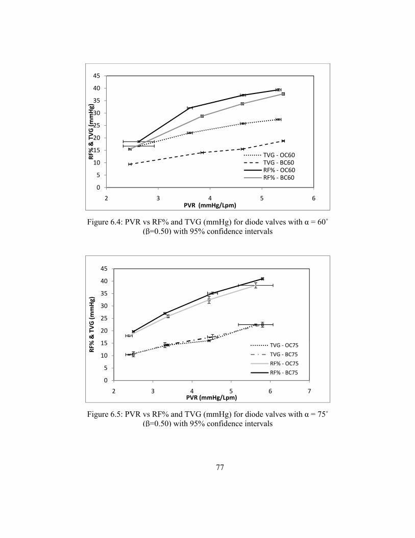
77
Figure 6.5: PVR vs RF% and TVG (mmHg) for diode valves with α = 75˚ (β=0.50) with 95% confidence intervals
0
5
10
15
20
25
30
35
40
45
2 3 4 5 6 7
RF% & TVG (m
mHg)
PVR (mmHg/Lpm)
TVG ‐ OC75
TVG ‐ BC75
RF% ‐ OC75
RF% ‐ BC75
Figure 6.4: PVR vs RF% and TVG (mmHg) for diode valves with α = 60˚ (β=0.50) with 95% confidence intervals
0
5
10
15
20
25
30
35
40
45
2 3 4 5 6
RF% & TVG (m
mHg)
PVR (mmHg/Lpm)
TVG ‐ OC60TVG ‐ BC60RF% ‐ OC60RF% ‐ BC60

78
Figure 6.7: PVR vs TVG for open cusped diode valve with different beta ratios. 95% confidence interval included. Tests conducted at cardiac output of 4 Lpm.
0
10
20
30
40
50
60
70
2 3 4 5 6
TVG (m
mHg)
PVR (mmHg/Lpm)
beta = 0.40beta = 0.45beta = 0.50
Figure 6.6: PVR vs RF% and TVG (mmHg) for diode valves with α = 90˚ (β=0.50) with 95% confidence intervals
0
5
10
15
20
25
30
35
40
45
2 3 4 5 6
RF% & TVG (m
mHg)
PVR (mmHg/Lpm)
TVG ‐ OC90
TVG ‐ BC90
RF% ‐ OC90
RF% ‐ BC90

79
Figure 6.8: PVR vs RF% for open cusped diodes valve with different beta ratios. 95% confidence intervals included.
0
5
10
15
20
25
30
35
40
45
50
2 3 4 5 6
RF%
PVR (mmHg/Lpm)
beta = 0.50beta = 0.40beta = 0.45

80
CHAPTER SEVEN
PARTICLE IMAGE VELOCIMETRY RESULTS
Particle image velocimetry was used to gather flow data in an open cusped diode
design and a backchannel diode. The diodes were machined in stainless steel and
polished. The details on each design are shown in Table 2.1 as designs 1 and 2.
Effect of Inertance
Inertance is the measure of the pressure gradient required to accelerate a fluid. It
is a function of the density of the fluid, the length and cross sectional area of the tubing in
which it flows. The following equation is the inertance for a tube:
I (19)
Inertance is related to the pressure gradient and the change in flow rate by equation 20.
∆ (20)
It was believed that the inertance in the mock circulatory system had an effect of
on the performance of the diode valve in the MPCS. This became of interest since the
PIV studies were performed with a blood analog with a higher density than the
performance studies. Higher inertance was believed to reduce the regurgitant fraction at
a given PVR. This concept was studied using an in house algorithm developed in

81
Matlab®. The algorithm simulated the MPCS in lumped parameter terms. Every
component of the physical system was represented in the lumped parameter model
(LPM). A schematic of the system upstream of the diode valve is shown in Figure 7.1.
The resistance, compliance and inertance elements were all identified. The upstream
inertance is depicted as LVH. A complete explanation of the algorithm is in Appendix A.
Using this model, the inertance (LVH) was varied and the resulting PVR, PVC,
TVG and RF% were found. The system inertance based on using water/glycerin and the
standard amount of ventricle hose used in the system was found to be 0.088 mmHg-s/mL.
The simulation was run at a PVR = 3.0 mmHg/Lpm and a cardiac output of 5.3 Lpm. The
resulting RF% was 11.1%. The ventricle inertance was reduced by a factor of 2, 4 and 8
and the RF% did not change. Decreasing the ventricle hose length below the standard had
no effect on the RF%. This suggested that standard hose length was acceptable.
The model was also run using levels of ventricle hose inertance greater than 0.088
mmHg-s/mL. As the inertance was increased, the RF% decreased. When LVH was raised
by 70%, the RF% decreased to 8.6%. Since the density of the water/glycerin/NaI blood
analog used in the PIV studies was 1.5 times higher than the water/glycerin solution, the
inertance was also 1.5 times higher. A table with complete results from the simulation is
located in Appendix A.

82
The results from the model support the conjecture that the RF% in a system using
the NaI solution would be lower than the RF% of a system using just water/glycerin at
the same resistance. Thus, the following PIV results have lower RF% for given values of
PVR. For example, in the parametric study, the RF% for the backchannel diode with a 60
angle at PVR = 5.4 mmHg/Lpm was 38% (Figure 6.2). However, in this study for the
same valve the RF% = 30% for a PVR of 6.85 mmHg/Lpm.
Determination of Time Delays
The accuracy of the particle image velocimetry measurements is dependent upon
the time between the two illumination pulses. A delay needs to be long enough so that
the displacement of the particles is determinable, but short enough to avoid particles with
an out-of-plane velocity component leaving the light sheet between subsequent
Figure 7.1. Lumped parameter model for the upstream of the Mock Circulatory System.
+PSV
Rbig Lbig
QTC "Tricuspid" ball check valve
Cbag
CRV
PVC
VH
Harvard Pump Cylinder
Ventricle Chamber
QVH
RVH LVH
Cb
RVP
Q
Diode Inlet

83
illuminations [118]. In this study, the time delay, ∆t in microseconds, varied for each
time step of the cardiac cycle and for each PVR tuning. The flow rate of each PVR
settings was recorded. The magnitude was checked in 50 ms intervals beginning with the
start of systole. This flow rate was converted from liters/minute to an equivalent average
velocity. The pixel calibration was used to determine a ∆t that corresponded with a
particle movement of roughly 10 pixels. The time delay accuracy was checked by
comparing the flow rate measured experimentally with the electromagnetic flow probe
with the calculated flow rate using the PIV results. At a particular time step, the average
velocity was found by performing a numerical integration on lines of constant x values.
Discussion of Data Sets
The plane of view for the particle image velocimetry was an overhead view that
captured the artery section just downstream of the valve as well as the pulmonary artery
branch. The central plane was grabbed without issue and the full area as shown in Figure
7.2. The laser sheet for the offset planes did not light the pulmonary branch sufficiently.
Most likely this was a result of the minor mismatch in the refractive indices. Therefore,
the full view of the pulmonary artery branch will be presented for the central plane;
however, only data from the main pulmonary artery will be presented for the offset
planes.
The PIV results for the two diode types are present here. The diodes were tested
at four different PVR levels of ~3 mmHg/Lpm, ~4 mmHg/Lpm, ~5 mmHg/Lpm and ~6
mmHg/Lpm and will be referred to as Cases 1 - 4. For each case, four of the 16 time
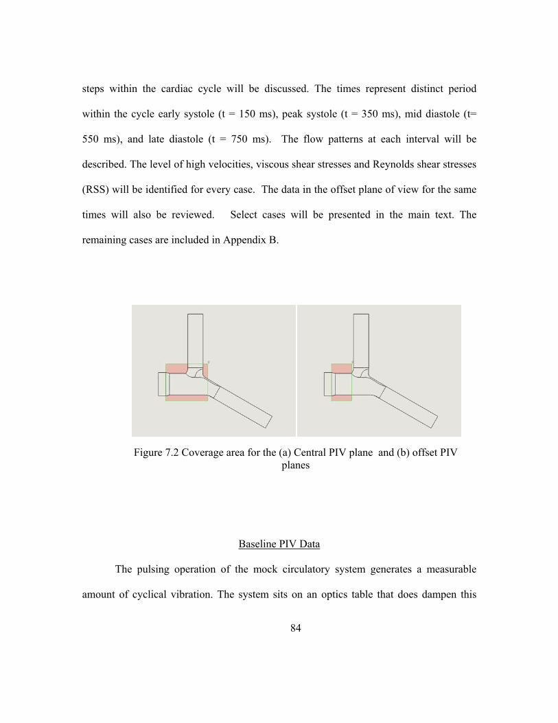
84
steps within the cardiac cycle will be discussed. The times represent distinct period
within the cycle early systole (t = 150 ms), peak systole (t = 350 ms), mid diastole (t=
550 ms), and late diastole (t = 750 ms). The flow patterns at each interval will be
described. The level of high velocities, viscous shear stresses and Reynolds shear stresses
(RSS) will be identified for every case. The data in the offset plane of view for the same
times will also be reviewed. Select cases will be presented in the main text. The
remaining cases are included in Appendix B.
Baseline PIV Data
The pulsing operation of the mock circulatory system generates a measurable
amount of cyclical vibration. The system sits on an optics table that does dampen this
Figure 7.2 Coverage area for the (a) Central PIV plane and (b) offset PIV planes

85
vibration; however, some residual vibration may exist. Since any movement in the
camera or the test section can affect the time values of the PIV measurements, a method
to determine the amount of this ‘noise’ was established.
The ‘noise’ resulting from any uncertainty in the PIV measurement was
ascertained by measuring a zero flow case to determine the effects of the system
operation on the measurements themselves. To do this, valves immediately upstream and
downstream of the test section were closed. However, the system otherwise operated
normally. The pulse rate of 75 bpm was applied to the ventricle by the mechanical pump
and fluid was circulated to the head tanks via the circulation pump. Measurements were
acquired normally and analyzed. Peak Reynolds shear stresses of up 2 dynes/cm2 were
created by the system effects. Peak viscous shear stresses of up to 1.45 dynes/cm2 were
observed in the same case. Yet, the average values were significantly lower. The mean
turbulent and viscous shear stresses were on the order of 0.1 dynes/cm2 and 0.07
dynes/cm2, respectively. These values are taken as the upper limits of noise due to
vibration on the acquired data.
Open Cusped Diode Results
Tests were run on the 25 mm open cusp diode. The system was adjusted to 75
bpm with an average flow rate of 5 Lpm. The pulmonary vascular resistance (PVR) of the
MCPS was regulated and set to achieve varying levels of RF%. The results for three
PVR values will be presented. They are: Case 1 - PVR = 3.1 mmHg/Lpm, Case 3- PVR =
5.1 mmHg/Lpm, and Case 4 - PVR = 6.1 mmHg/Lpm. The central plane PIV results will

86
be discussed for all three cases. Only the Case 1 offset plane results will be discussed in
detail here. The remaining results discussion is in Appendix B.
Case 1
The pressure and flow curve for the low case of PVR = 3.1 mmHg/Lpm is shown
in Figure 7.3. The regurgitant fraction for this circumstance is 1.84%. The PIV results
show that flow patterns throughout the cardiac cycle. First, the results from the central
plane are presented.
Early systole (t = 150 ms)
During early systole, uniform antegrade flow exists the main arterial section Flow
is seen in the arterial branches as well. It is relatively undisturbed in the left pulmonary
artery (LPA) in comparison to the right. . The velocities in the main pulmonary artery
(MPA) range between 0 – 0.15 m/s with an average of 0.08 m/s.
Figure 7.4 also shows the hydraulic shear stresses for this case. The uniform flow
profile results in the highest stresses being near the walls. The magnitudes of these
stresses are under 5 dynes/cm2. However, statistical analysis shows that these values are
significantly different than those measured in the baseline case suggesting that the values
are valid.
At 150 ms after the start of systole there is little disturbance in the flow. The peak
shear stresses are at the RPA branch where MPA axial flow is moving around the 90°
arterial bend and in the middle of the bifurcation where the primary and secondary flows
87
meet (Figure 7.4). The RSS are low in comparison to the rest of the cardiac cycle and
this is shown in Figure 7.5.
Peak systole (t = 350 ms)
The jet develops and moves downstream through the MPA reaching the RPA and
LPA branches by 200 ms after the start of systole. It continues to accelerate downstream
for another 150 ms. The highest flow rate, considered to be peak systole, occurs between
350 and 400 ms after the start of systole. Figure 7.6 shows the flow and shear stress
fields at 350 ms. The entrained region is defined by moving vortical cells traveling along
the MPA wall leaving behind region of recirculation from r = ±7 mm to ±11.5 mm as
shown in Figure 7.6. As the jet entrainment vortex forms around the central core a region
of recirculation is seen to form as the flow diverges into the right pulmonary artery
(RPA). The jet impinges on the artery wall at the bifurcation. The maximum velocity at
this point in the cardiac cycle is 1.28 m/s and the average velocity is 0.410 m/s. In the
RPA, the velocities are highest along the outer wall (more downstream) and weaken
toward the inner wall. Along the outer wall, the velocities are on the order of 0.400 m/s.
The peak viscous shear stresses for this case are approximately 30 dynes/cm2
(Figure 7.6). The wall shear stresses along the outer RPA wall are around 15 dynes/cm2,
which is relatively high in comparison to the rest of the field.
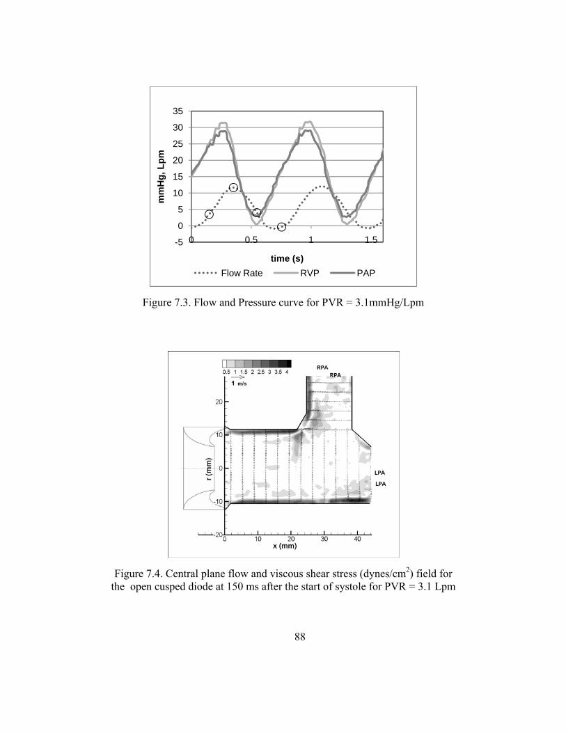
88
Figure 7.4. Central plane flow and viscous shear stress (dynes/cm2) field for the open cusped diode at 150 ms after the start of systole for PVR = 3.1 Lpm
Figure 7.3. Flow and Pressure curve for PVR = 3.1mmHg/Lpm
-5
0
5
10
15
20
25
30
35
0 0.5 1 1.5
mm
Hg,
Lpm
time (s)Flow Rate RVP PAP
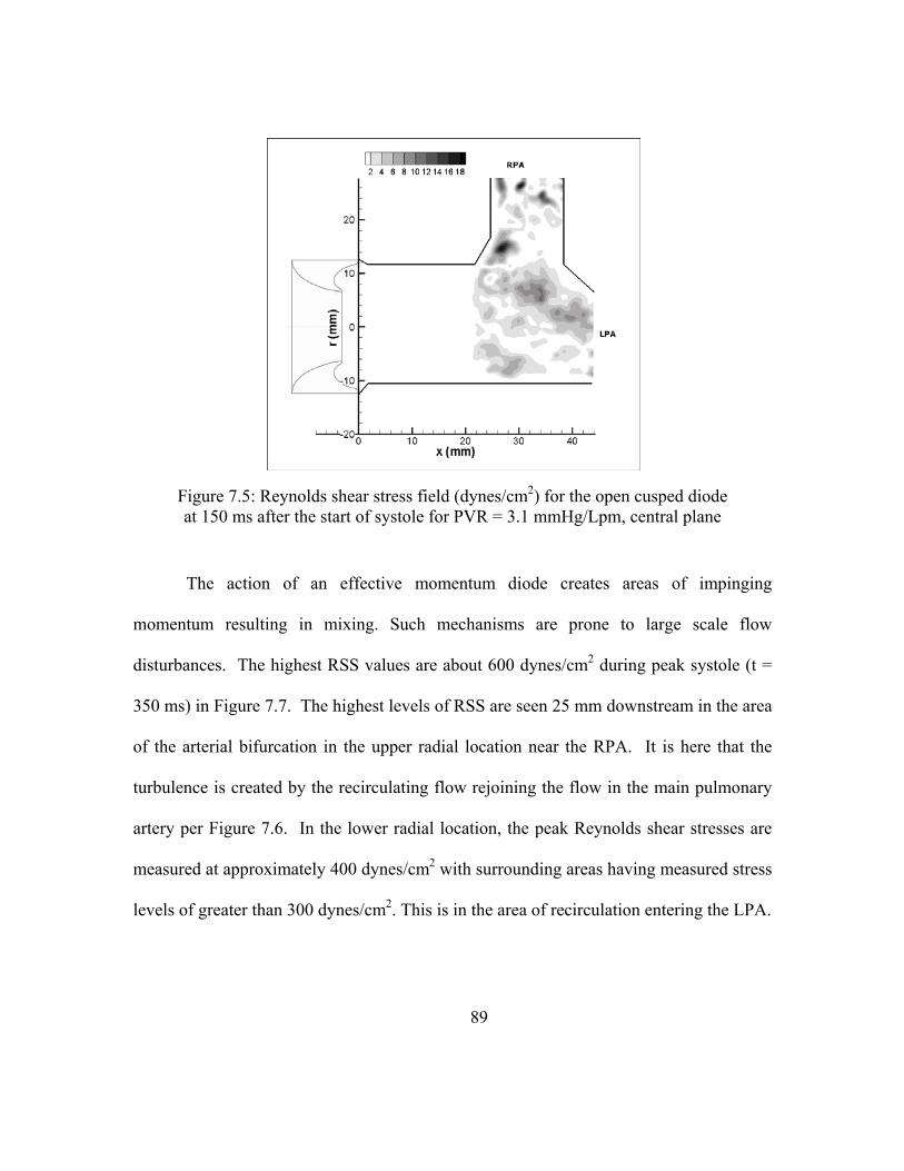
89
The action of an effective momentum diode creates areas of impinging
momentum resulting in mixing. Such mechanisms are prone to large scale flow
disturbances. The highest RSS values are about 600 dynes/cm2 during peak systole (t =
350 ms) in Figure 7.7. The highest levels of RSS are seen 25 mm downstream in the area
of the arterial bifurcation in the upper radial location near the RPA. It is here that the
turbulence is created by the recirculating flow rejoining the flow in the main pulmonary
artery per Figure 7.6. In the lower radial location, the peak Reynolds shear stresses are
measured at approximately 400 dynes/cm2 with surrounding areas having measured stress
levels of greater than 300 dynes/cm2. This is in the area of recirculation entering the LPA.
Figure 7.5: Reynolds shear stress field (dynes/cm2) for the open cusped diode at 150 ms after the start of systole for PVR = 3.1 mmHg/Lpm, central plane

90
Mid Diastole (t = 550 ms)
Figure 7.8 shows the flow and viscous shear stresses near the peak mid diastole
phase (t = 550 ms). The jet structure can still be discerned with peak velocities not less
than about 0.6 m/s, and with an average velocity of 0.186 m/s. At the outer RPA, the
velocities are still slightly above 0.400 m/s. The region of recirculating flow is still
present as flow momentum has carried it into the right and left pulmonary arteries.
The bulk shear stresses are still the highest along the edges of the central jet
shown in Figure 7.8. The values are about 15 dynes/cm2, half that observed at peak
systole (just as the velocities were). The wall shear stresses in the RPA, however, are
unchanged at approximately 15 dynes/cm2 since the velocities also remained the same
during this time interval.
Figure 7.9 shows the RSS field and the peak RSS measurements take place where
the flow diverges into the RPA and LPA. Moreover, in the area in which the secondary
RPA flow wraps around and meets the MPA flow, the Reynolds shear stresses have
lessened to around 200 dynes/cm2. The area of recirculating flow leading into the LPA,
however, remains disturbed and has turbulent shear stress values of 200-300 dynes/cm2.

91
Figure 7.7: Reynolds shear stress field (dynes/cm2) for the open cusped diode at 350 ms after the start of systole for PVR = 3.1 mmHg/Lpm, central plane
Figure 7.6: Central plane flow and viscous shear stress (dynes/cm2) field for the open cusped diode at 350 ms after the start of systole for PVR = 3.1 Lpm

92
Late Diastole (t = 750 ms)
Finally, Figure 7.10 shows the flow region during mid-diastole at 750 ms after the
start of systole. By this point in the cycle the retrograde flow is established throughout
the test section. The velocity profile is uniform as the branch flow converges in the main
PA; the average flow is about -0.072 m/s across the test section. This corresponds with
the negative flow rate measured between 620 – 800 ms (Figure 7.3). The retrograde
motion is well behaved and allows the flow to wash artery walls and eliminate regions of
recirculation. Only at the region of the bifurcation is stasis flow measured. The wall
stresses are less than 5 dynes/cm2. This is consistent with the uniform flow.
Figure 7.11 shows the field of turbulent shear stresses. The peak stresses are less
than 50 dynes/cm2. These measured stresses are well above the noise measured in the
zero flow case thus suggesting that the 50 dynes/cm2 is reflective of the turbulent shear
stresses in the flow.
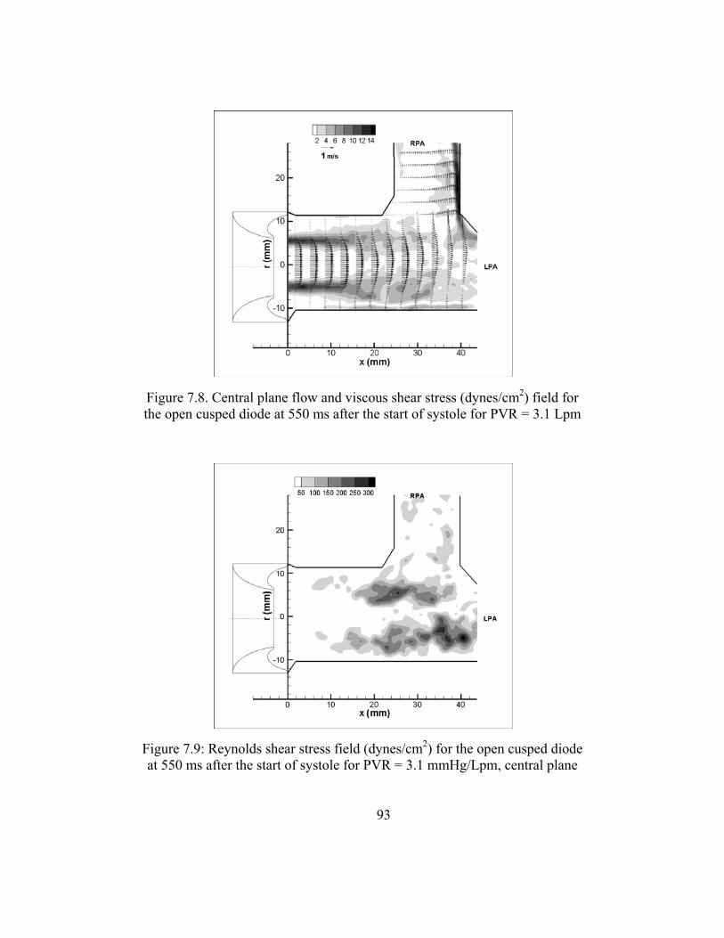
93
Figure 7.9: Reynolds shear stress field (dynes/cm2) for the open cusped diode at 550 ms after the start of systole for PVR = 3.1 mmHg/Lpm, central plane
Figure 7.8. Central plane flow and viscous shear stress (dynes/cm2) field for the open cusped diode at 550 ms after the start of systole for PVR = 3.1 Lpm

94
Figure 7.11: Reynolds shear stress field (dynes/cm2) for the open cusped diode at 750 ms after the start of systole for PVR = 3.1 mmHg/Lpm, central plane
Figure 7.10. Central plane flow and viscous shear stress (dynes/cm2) field for the open cusped diode at 750 ms after the start of systole for PVR = 3.1 Lpm
95
Case 1 - Offset planes
The offset flow plane was 5 mm from the central plane. Therefore, the radius of
the cross section in this view is 10.75 mm versus the 11.85 mm measured in the central
plane. The offset flow plane has similar characteristics as the central plane. Also, in the
offset plane of view, the laser sheet did not adequately light the arterial branches.
Therefore, the field of view is only the main artery.
Early systole (t = 150 ms)
At 150 ms after the start of the cycle (Figure 7.12) the velocities are on the order
of -0.0440 m/s with maximum values of 0.102 m/s. As time progresses, the jet flow
emerges from the diode valve. The width of the jet is expectedly narrower than that
along the central plane of pulmonary artery. Vortical structures are present, and begin
approximately 6.5 mm away from the axial centerline in both radial directions.
The viscous stresses in the offset planes were analyzed for comparison to the
central plane data (Figure 7.12). The data from both planes are similar in trend and
magnitude. The wall shear stresses are approximately 3.7 dynes/cm2. This is of similar
magnitude as the wall shear stresses seen in the central plane (Figure 7.4).
As with the viscous shear stresses, there is little difference between the Reynolds
shear stress fields in the offset and central planes. However, since the more notable
turbulent shear stresses in the central plane fields occur more than 20 mm downstream
the offset plane data is abbreviated and does not have as much detail. In Figure 7.13,

96
RSS map for the early systole case is shown. The peak turbulent stresses within the first
22 mm of the diode are on the order of 5 dynes/cm2.
Peak systole (t = 350 ms)
These areas are well defined during peak systole, 350 ms after the start of the
cycle, as seen in Figure 7.14. The average and peak velocities at this phase were found to
be 0.308 m/s and 1.17 m/s, respectively. The peak shear stresses occur along the edge of
the jet structure with values of 28 dynes/cm2. At 350 ms after the start of systole, the
magnitudes are on the same level observed in the central plane (within 22 mm of the
valve exit). As seen in Figure 7.15, the peak turbulent stresses are 330 dynes/cm2.
Mid Diastole (t = 550 ms)
Figure 7.16 shows the flow at mid diastole. The velocity is still dependent on the
radial location. The maximum velocity is 0.545 m/s which is about half of what was seen
at peak systole. The average velocity is 0.129 m/s. The peak stresses are along the edges
of the centrally formed jet. The peak values are 10 dynes/cm2. Likewise, at 550 ms into
the cycle the RSS fields are similar for the offset and central planes. The stresses reach
up to 143 dynes/cm2. This can be seen by comparing Figure 7.9 and Figure 7.17.
Late Diastole (t = 750 ms)
During diastole the velocities are on the order of -0.075 m/s and are relatively
uniform (Figure 7.18). The axial velocity peaks at -0.152 m/s. The wall shear stresses are
just below 4 dynes/cm2 during diastole, 750 ms after the start of the cycle. All of these

97
offset measurements are similar to the central plane measurements. The offset plane RSS
measurements are shown in Figure 7.19. There is little disturbance; the turbulent shear
stresses are in the range of 22 dynes/cm2.
Case 3
The pressure and flow curves for the open cusped diode at this setting are shown
in Figure 7.20. The flow rates vary from -4.5 Lpm to 16 Lpm. The four 150 ms time
intervals are marked off with circles. At 350 ms into the cycle, the peak flow rate has not
been reached. Peak systole takes places at 450 ms and is also denoted on the flow curve.
Therefore, for this instance, five points will be presented. The pulmonary vascular
resistance is 5.1 mmHg/Lpm and the RF% is 18%.
Figure 7.12. Offset plane flow and viscous shear stress (dynes/cm2) field for the open cusped diode at 150 ms after the start of systole for PVR = 3.1 Lpm
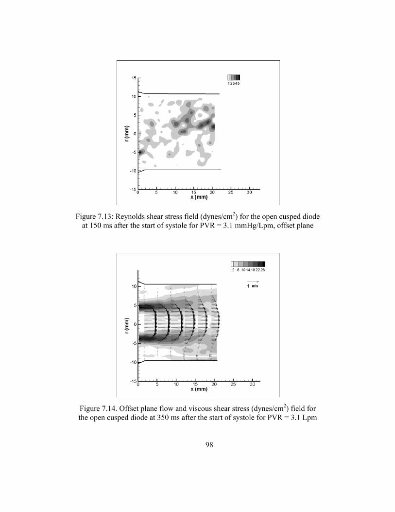
98
Figure 7.14. Offset plane flow and viscous shear stress (dynes/cm2) field for the open cusped diode at 350 ms after the start of systole for PVR = 3.1 Lpm
Figure 7.13: Reynolds shear stress field (dynes/cm2) for the open cusped diode at 150 ms after the start of systole for PVR = 3.1 mmHg/Lpm, offset plane
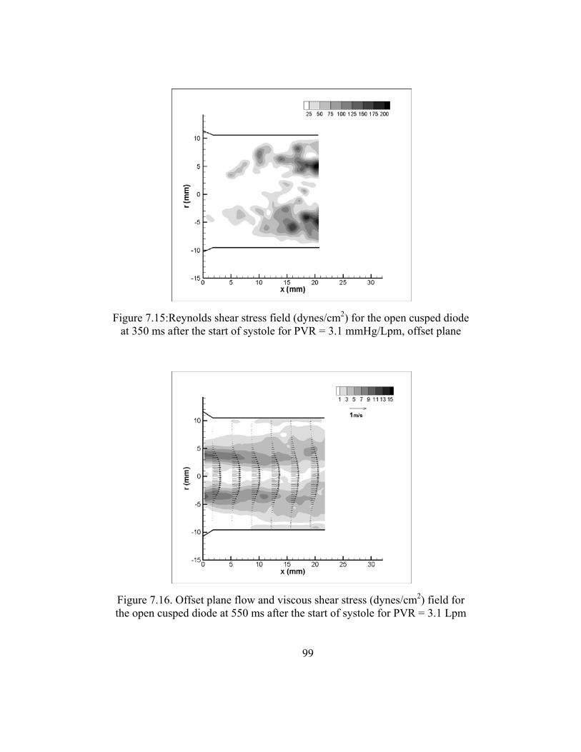
99
Figure 7.16. Offset plane flow and viscous shear stress (dynes/cm2) field for the open cusped diode at 550 ms after the start of systole for PVR = 3.1 Lpm
Figure 7.15:Reynolds shear stress field (dynes/cm2) for the open cusped diode at 350 ms after the start of systole for PVR = 3.1 mmHg/Lpm, offset plane
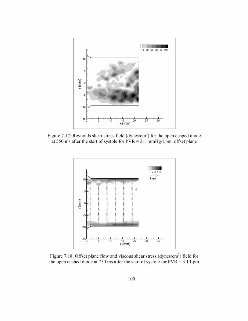
100
Figure 7.18. Offset plane flow and viscous shear stress (dynes/cm2) field for the open cushed diode at 750 ms after the start of systole for PVR = 3.1 Lpm
Figure 7.17: Reynolds shear stress field (dynes/cm2) for the open cusped diode at 550 ms after the start of systole for PVR = 3.1 mmHg/Lpm, offset plane
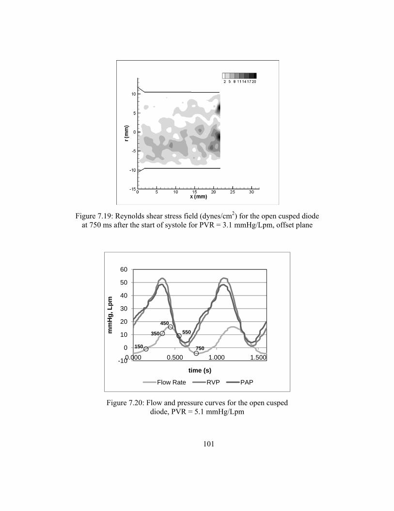
101
Figure 7.20: Flow and pressure curves for the open cusped diode, PVR = 5.1 mmHg/Lpm
150
350
450550
750
-10
0
10
20
30
40
50
60
0.000 0.500 1.000 1.500
mm
Hg,
Lpm
time (s)
Flow Rate RVP PAP
Figure 7.19: Reynolds shear stress field (dynes/cm2) for the open cusped diode at 750 ms after the start of systole for PVR = 3.1 mmHg/Lpm, offset plane

102
Early Systole (t = 150 ms)
Figure 7.21 is the flow profile at 150 ms for the PVR = 5.1 mmHg/Lpm case with
axial and radial vector spacing, respectively. Unlike the Cases 1 and 2, the flow at this
point is still transitioning from retrograde to antegrade. Uniform reverse flow exists in
the right and left pulmonary arteries. The two flows combine and form reverse axial flow
in the main artery. The peak reverse velocity is about 0.186 m/s and the average velocity
in the main pulmonary artery is -0.208 m/s.
The bulk flow shear stresses are overall very low at 150 ms after the beginning of
systole. The peak stresses within the field reach 2-3 dynes/cm2 along the regions of
recirculation (Figure 7.21). The peak wall shear stresses are in the RPA at 4 - 5
dynes/cm2 resulting from the reverse flow.
The turbulence shear stresses for the field at 150 ms after the start of systole are
shown in Figure 7.22. The peak RSS values are 130 dynes/cm2. This is higher than they
were in the PVR = 4.3 case at 150 ms (50 dynes/cm2). Figure 7.21 shows jet flow
emerging from the RPA into the path of the LPA retrograde flow. The RPA flow has
more momentum than at lower PVR values; thus, there is more mixing and more
turbulence. The region of peak turbulent shear stresses is isolated at 32 mm downstream
and about 3.5 above the centerline. There is no measureable RSS in the regions of stasis
flow.

103
Figure 7.22: Reynolds shear stress field (dynes/cm2) for the open cusped diode at 150 ms after the start of systole for PVR = 5.1 mmHg/Lpm, central plane
Figure 7.21: Central plane flow and viscous shear stress (dynes/cm2) field for the open cusped diode at 150 ms after the start of systole for PVR = 5.1 mmHg/Lpm

104
Mid systole (t = 350 ms)
During mid systole, a central jet is observed to exit the valve, travel into the LPA
and impinge on the wall of the LPA as seen in Figure 7.23. There are rolling vortices in
the main artery, the larger of the two at the lower MPA wall. The flow in the right artery
has strong axial component along the distal wall. This is more like the flows at the low
PVR = 3.1 mmHg/Lpm case as opposed to the PVR = 4.3 mmHg/Lpm case where the
primary flow makes a relatively smooth turn into the RPA. In the left pulmonary artery
the jet structure flows mostly unimpeded. The area of recirculation ends at the LPA
entrance, near 32 mm downstream. The maximum velocity magnitudes are 1.63 m/s.
The average axial velocity in the MPA is 0.576 m/s.
The highest bulk flow shear stresses are along the edges of the jet (Figure 7.23).
This is similar to what occurs during peak systole at lower PVR values. The peak
stresses measure approximately 45 dynes/cm2. The wall shear stresses along the distal
RPA wall are just over 16 dynes/cm2. Also, the viscous stresses along lower LPA wall
where the flow reattaches are about 14 dynes/cm2.
The Reynolds shear stress field for the PVR = 5.1 mmHg/Lpm during mid systole
is shown in Figure 7.24. The values range from 0 to 700 dynes/cm2. The peak at 700
dynes/cm2 is at the bend between the right and main arteries where flow separation takes
place. The Reynolds shear stresses measures ~300 dynes/cm2 in the area of recirculation
in the RPA and entering the LPA.

105
Figure 7.24: Reynolds shear stress field (dynes/cm2) for the open cusped diode at 350 ms after the start of systole for PVR = 5.1 mmHg/Lpm, central plane
Figure 7.23: Central plane flow and viscous shear stress (dynes/cm2) field for the open cusped diode at 350 ms after the start of systole for PVR = 5.1 mmHg/Lpm

106
Peak Systole (t = 450 ms)
The peak flow rate occurs 450 ms after the start of systole. The flow and viscous
shear stress fields are shown in Figure 7.25. The entrained jet structure is well developed.
It travels into the LPA and impinges on the wall of that artery branch. The average
velocity in the main pulmonary artery is 0.583 m/s. the velocity peaks at 1.65 m/s. The
flow profile in the RPA is skewed to the distal wall where velocities measure up to 1.0
m/s.
The highest bulk flow shear stresses are along the edges of the jet (Figure 7.25).
The peak stresses again measure approximately 45 dynes/cm2. The wall shear stresses at
the site of impingement where the flow diverges are approximately 22 dynes/cm2. The
viscous stresses along the distal RPA wall and the lower LPA wall where the flow
reattaches are about 10 dynes/cm2.
Figure 7.26 is the Reynolds shear stresses field at peak systole. The
measurements peak at 1100 dynes/cm2. The peak Reynolds shear stress is approximately
650 dynes/cm2 in the area that the recirculating flow rejoins the primary flow in the
MPA. This region of disturbance has travelled downstream to about 30 mm from the
valve exit. Another area of high RSS is in the lower radial location near the MPA and
LPA branch where they reach their highest value of 1100 dynes/cm2 at this point.
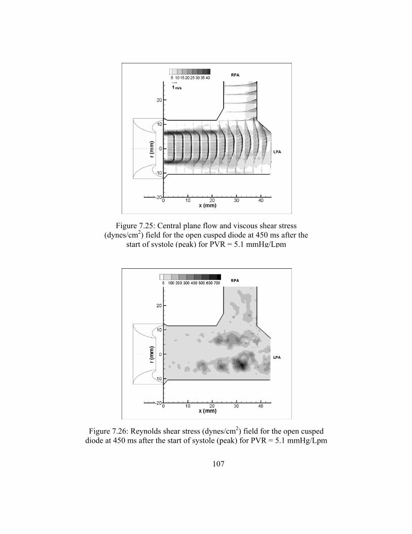
107
Figure 7.26: Reynolds shear stress (dynes/cm2) field for the open cusped diode at 450 ms after the start of systole (peak) for PVR = 5.1 mmHg/Lpm
Figure 7.25: Central plane flow and viscous shear stress (dynes/cm2) field for the open cusped diode at 450 ms after the
start of systole (peak) for PVR = 5.1 mmHg/Lpm

108
Mid Diastole (t= 550 ms)
Figure 7.27 shows the flow and bulk shear stress profiles at mid diastole. The
secondary flow from the right pulmonary artery is recirculating into the main branch.
The region of flow separation along the lower MPA and LPA walls has lengthened. The
highest velocities are about 0.881 m/s, one half of the velocities measured during peak
systole. The average velocity in the main artery is about half of the peak systole average
velocity at 0.282 m/s.
As with the earlier described cases, at 550 ms after the start of the cycle, the bulk
shear stresses are still the highest along the edges of the central jet with values up to 23
dynes/cm2 as seen in Figure 7.27. The shear layer has extended as the area of flow
separation lengthened. Moreover, the wall shear stresses in the RPA are between 14 – 20
dynes/cm2.
In Figure 7.28, the RSS field for 550 ms after the start of systole is shown. The
turbulent stresses reach as high as 700 dynes/cm2 during mid diastole. It is higher where
flow develops near the LPA entry (Figure B.6). The stresses are approximately 300
dynes/cm2 where the RPA recirculating flow and the MPA flow converge.
Late Diastole (t = 750 ms)
At the 750 ms after the systolic start, there is prevalent retrograde flow in the
entire pulmonary artery (Figure 7.29). The peak velocities are about -0.500 m/s and
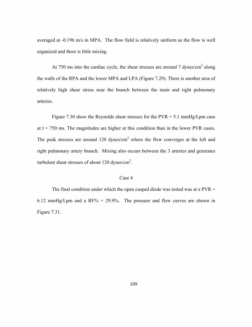
109
averaged at -0.196 m/s in MPA. The flow field is relatively uniform as the flow is well
organized and there is little mixing.
At 750 ms into the cardiac cycle, the shear stresses are around 7 dynes/cm2 along
the walls of the RPA and the lower MPA and LPA (Figure 7.29). There is another area of
relatively high shear stress near the branch between the main and right pulmonary
arteries.
Figure 7.30 show the Reynolds shear stresses for the PVR = 5.1 mmHg/Lpm case
at t = 750 ms. The magnitudes are higher at this condition than in the lower PVR cases.
The peak stresses are around 120 dynes/cm2 where the flow converges at the left and
right pulmonary artery branch. Mixing also occurs between the 3 arteries and generates
turbulent shear stresses of about 120 dynes/cm2.
Case 4
The final condition under which the open cusped diode was tested was at a PVR =
6.12 mmHg/Lpm and a RF% = 29.9%. The pressure and flow curves are shown in
Figure 7.31.

110
Figure 7.28: Reynolds shear stress field (dynes/cm2) for the open cusped diode at 550 ms after the start of systole for PVR = 5.1 mmHg/Lpm, central plane
Figure 7.27: Central plane flow and viscous shear stress (dynes/cm2) field for the open cusped diode at 550 ms after the start of systole for PVR = 5.1 mmHg/Lpm

111
Figure 7.30: Reynolds shear stress field (dynes/cm2) for the open cusped diode at 750 ms after the start of systole for PVR = 5.1 mmHg/Lpm, central plane
Figure 7.29: Central plane flow and viscous shear stress (dynes/cm2) field for the open cusped diode at 750 ms after the start of systole for PVR = 5.1 mmHg/Lpm
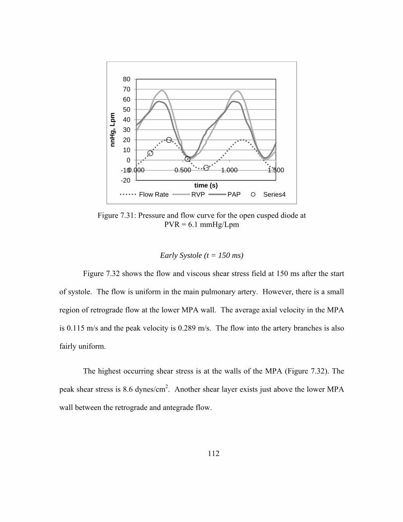
112
Early Systole (t = 150 ms)
Figure 7.32 shows the flow and viscous shear stress field at 150 ms after the start
of systole. The flow is uniform in the main pulmonary artery. However, there is a small
region of retrograde flow at the lower MPA wall. The average axial velocity in the MPA
is 0.115 m/s and the peak velocity is 0.289 m/s. The flow into the artery branches is also
fairly uniform.
The highest occurring shear stress is at the walls of the MPA (Figure 7.32). The
peak shear stress is 8.6 dynes/cm2. Another shear layer exists just above the lower MPA
wall between the retrograde and antegrade flow.
Figure 7.31: Pressure and flow curve for the open cusped diode at PVR = 6.1 mmHg/Lpm
-20-10
01020304050607080
0.000 0.500 1.000 1.500
nnH
g, L
pm
time (s)Flow Rate RVP PAP Series4
113
The turbulent shear stress field is plotted in Figure 7.33. The levels of turbulent
shear stress reach 65 dynes/cm2. One elevated region is near where flow from the main
artery turns in the right branch.
Peak Systole (t = 350 ms)
At the point of maximum flow rate, there is again a strong central jet present in
the flow field (Figure 7.34). There are areas of recirculation in both the upper and lower
part of the MPA. The jet flow strikes the artery wall at the bifurcation and extends well
into the left pulmonary artery. The flow in the RPA is skewed strongly toward the distal
wall as momentum carries the flow downstream. In the MPA, the average and maximum
flow speeds are 0.860 m/s and 2.37 m/s, respectively.
The highest bulk flow stresses are located along the jet edges (Figure 7.34). The
peak stresses are up to 55 dynes/cm2. The shear layer dissipates the central core flow
reaches the branch. The wall shear stresses at the distal RPA wall are as high as 10
dynes/cm2.
The Reynolds shear stresses for peak systole are shown in Figure 7.35. One of
the regions where high levels of disturbance take place is positioned in between the MPA
and RPA. This is where the primary flow begins to diverge and the peak values are as
high as 900 dynes/cm2. The point where the highest overall turbulent shear stress is
located is in the lower MPA and LPA in the area of recirculation. Here the RSS were
measured to be 1520 dynes/cm2.

114
Mid Diastole (t = 550 ms)
As the cycle progresses to 550 ms after the start of the cycle, the strength of the
central core jet has lessened (Figure 7.36). There are areas of recirculation in the upper
and lower MPA, in the LPA and in the RPA. The average velocity has decreased to
0.124 m/s and the maximum velocities are 0.487 m/s, nearly half of what they were at
peak systole.
Figure 7.36 also shows the hydraulic shear stresses in at this point in the cardiac
cycle. The flow gradient at the edges of the jet produces relatively high shear stresses.
Also, shear layers are present between the retrograde flow and the walls. The maximum
hydraulic shear stresses at this point are just under 9 dynes/cm2.
The highest Reynolds shear stresses are on the order of 340 dynes/cm2. Similar to
the RSS field at peak systole, there is a region of elevated stresses at the point when the
primary flow from the MPA is turning into the RPA. There is another area of mixing
about 35 mm downstream of the valve exit 4 mm below the center of the artery.

115
Figure 7.33: Reynolds shear stress (dynes/cm2) field for the open cusped diode at 150 ms after the start of systole for PVR = 6.1 mmHg/Lpm
Figure 7.32: Central plane flow and viscous shear stress (dynes/cm2) field for the open cusped diode at 150 ms after the start of systole for PVR 6.1 mmHg/Lpm
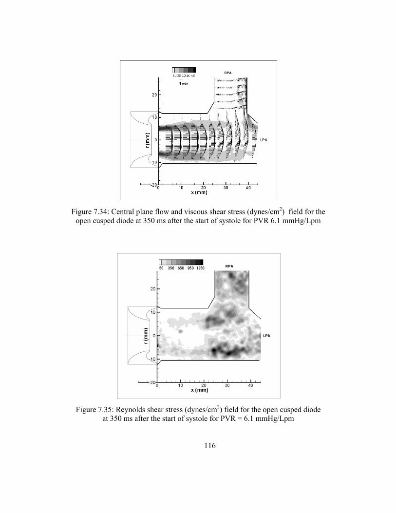
116
Figure 7.35: Reynolds shear stress (dynes/cm2) field for the open cusped diode at 350 ms after the start of systole for PVR = 6.1 mmHg/Lpm
Figure 7.34: Central plane flow and viscous shear stress (dynes/cm2) field for the open cusped diode at 350 ms after the start of systole for PVR 6.1 mmHg/Lpm
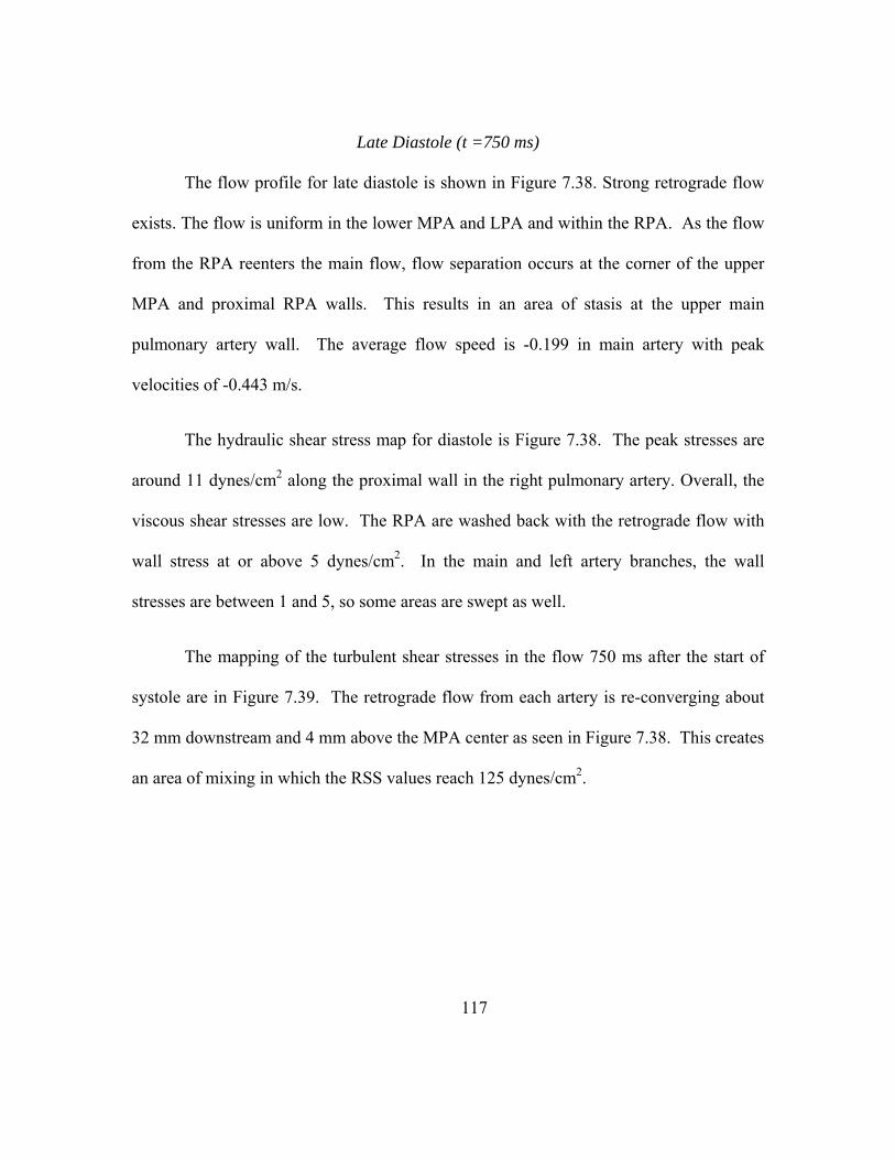
117
Late Diastole (t =750 ms)
The flow profile for late diastole is shown in Figure 7.38. Strong retrograde flow
exists. The flow is uniform in the lower MPA and LPA and within the RPA. As the flow
from the RPA reenters the main flow, flow separation occurs at the corner of the upper
MPA and proximal RPA walls. This results in an area of stasis at the upper main
pulmonary artery wall. The average flow speed is -0.199 in main artery with peak
velocities of -0.443 m/s.
The hydraulic shear stress map for diastole is Figure 7.38. The peak stresses are
around 11 dynes/cm2 along the proximal wall in the right pulmonary artery. Overall, the
viscous shear stresses are low. The RPA are washed back with the retrograde flow with
wall stress at or above 5 dynes/cm2. In the main and left artery branches, the wall
stresses are between 1 and 5, so some areas are swept as well.
The mapping of the turbulent shear stresses in the flow 750 ms after the start of
systole are in Figure 7.39. The retrograde flow from each artery is re-converging about
32 mm downstream and 4 mm above the MPA center as seen in Figure 7.38. This creates
an area of mixing in which the RSS values reach 125 dynes/cm2.

118
Figure 7.37: Reynolds shear stress (dynes/cm2) field for the open cusped diode at 550 ms after the start of systole for PVR = 6.1 mmHg/Lpm
Figure 7.36: Central plane flow and viscous shear stress (dynes/cm2) field for the open cusped diode at 550 ms after the start of systole for PVR 6.1 mmHg/Lpm
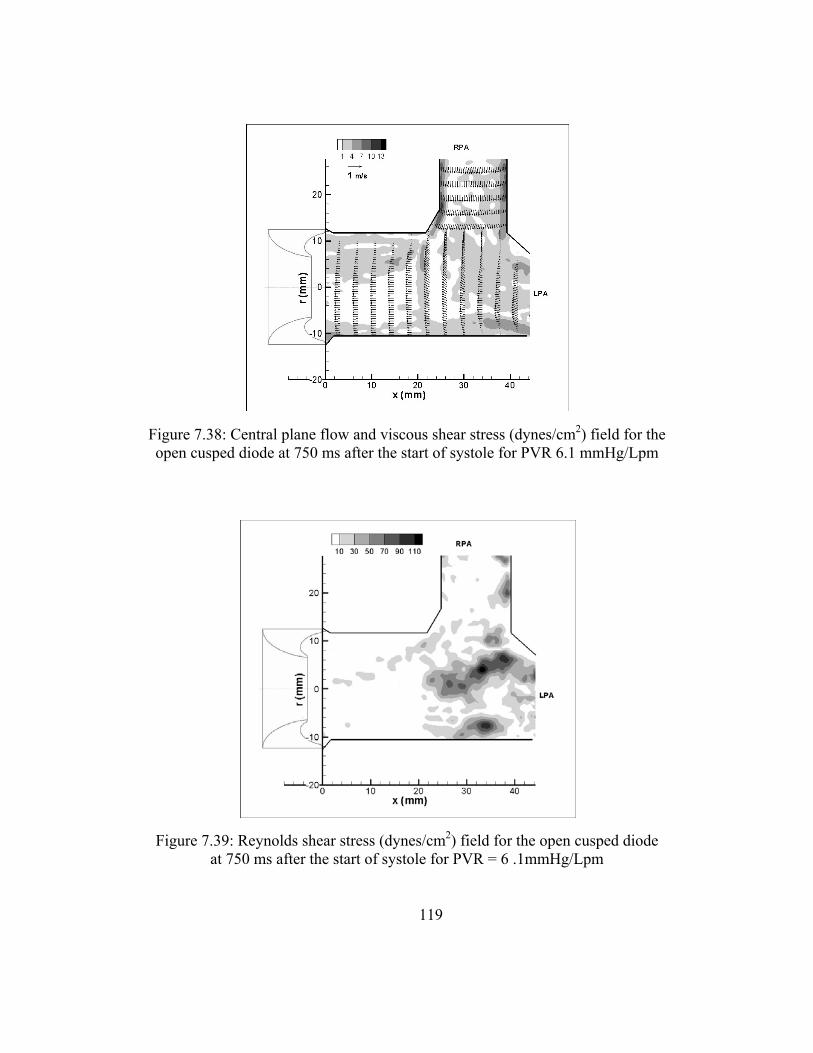
119
Figure 7.39: Reynolds shear stress (dynes/cm2) field for the open cusped diode at 750 ms after the start of systole for PVR = 6 .1mmHg/Lpm
Figure 7.38: Central plane flow and viscous shear stress (dynes/cm2) field for the open cusped diode at 750 ms after the start of systole for PVR 6.1 mmHg/Lpm
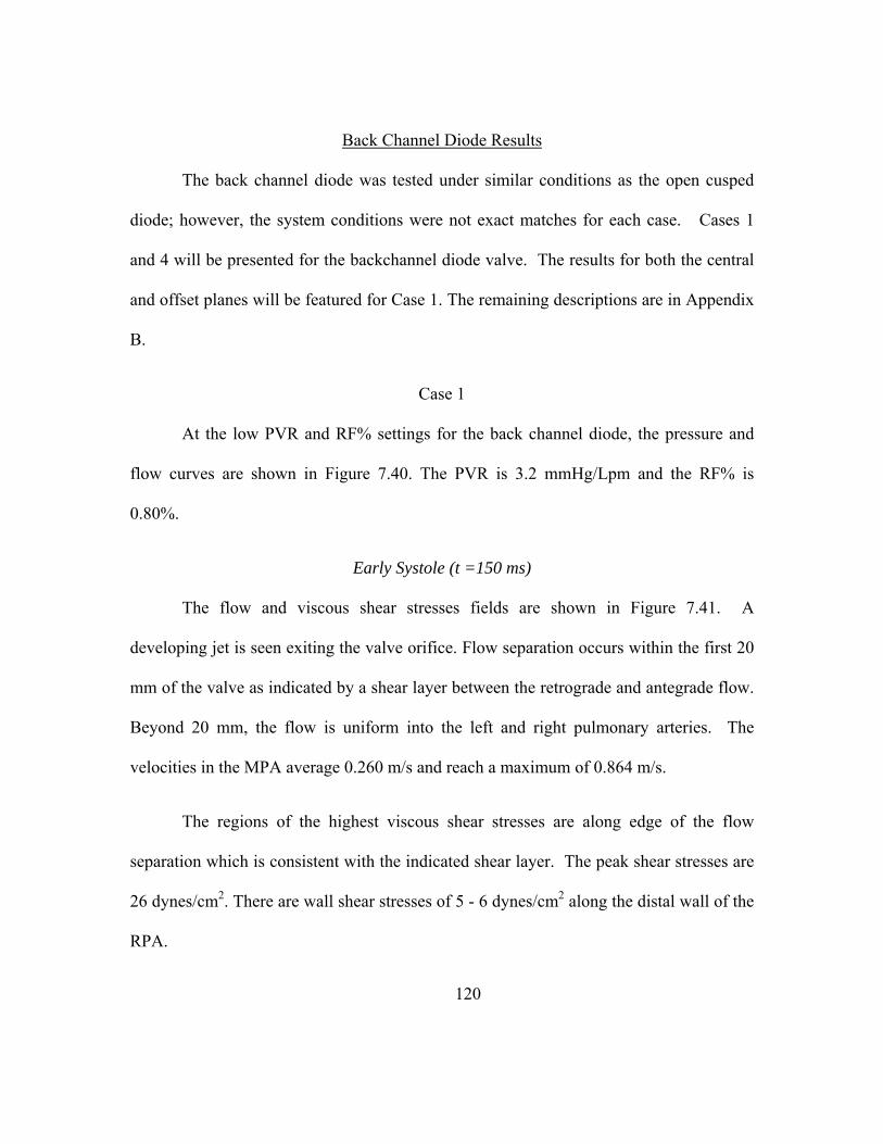
120
Back Channel Diode Results
The back channel diode was tested under similar conditions as the open cusped
diode; however, the system conditions were not exact matches for each case. Cases 1
and 4 will be presented for the backchannel diode valve. The results for both the central
and offset planes will be featured for Case 1. The remaining descriptions are in Appendix
B.
Case 1
At the low PVR and RF% settings for the back channel diode, the pressure and
flow curves are shown in Figure 7.40. The PVR is 3.2 mmHg/Lpm and the RF% is
0.80%.
Early Systole (t =150 ms)
The flow and viscous shear stresses fields are shown in Figure 7.41. A
developing jet is seen exiting the valve orifice. Flow separation occurs within the first 20
mm of the valve as indicated by a shear layer between the retrograde and antegrade flow.
Beyond 20 mm, the flow is uniform into the left and right pulmonary arteries. The
velocities in the MPA average 0.260 m/s and reach a maximum of 0.864 m/s.
The regions of the highest viscous shear stresses are along edge of the flow
separation which is consistent with the indicated shear layer. The peak shear stresses are
26 dynes/cm2. There are wall shear stresses of 5 - 6 dynes/cm2 along the distal wall of the
RPA.
121
The Reynolds shear stress field for the low PVR and RF% setting is shown in
Figure 7.42. The RSS levels within the flow field measure 40 dynes/cm2. At the valve
exit, there is observed noise with point of RSS measuring as high as 225 dynes/cm2. This
may be a result of uncertainty in the velocity vector determination at this point in the
field.
Peak systole (t = 350 ms)
The flow evolves into a developing jet as the cardiac cycle progresses to reach
peak systole as a retrograde vortex moves across the artery walls (Figure 7.43). The core
jet is well defined downstream of valve and into the LPA. The flow separates at the inner
wall of the RPA branch, and a region of recirculation is present resulting in larger
velocities along the outer wall. The peak velocity is 1.52 m/s and in the MPA, the
average is 0.445 m/s.

122
Figure 7.41: Central plane flow and viscous shear stress (dynes/cm2) field for the backchannel diode at 150 ms after the start of systole for PVR = 3.2 mmHg/Lpm
Figure 7.40: Pressure and flow curve for backchannel diode at PVR = 3.2 mmHg/Lpm
-5
0
5
10
15
20
25
30
35
0 0.5 1 1.5
mm
Hg
and
Lpm
time(s)flow rate (lpm) PAP (mmHg) RVP (mmHg)

123
Expectedly, the viscous shear stresses have increased as the shear layer has
extended. Along the edges of the central core jet, the stresses peak 45 dynes/cm2. The
stresses along the distal RPA wall are as high as 27 dynes/cm2. Along the lower MPA
and into the LPA, the existence of retrograde flow leads to wall stresses of 10 - 14
dynes/cm2.
Figure 7.44 shows the Reynolds shear at peak systole for Case 4. The regions of
highest turbulence coincide with the areas of recirculation. One area, located about 6 mm
off center in the lower MPA, has RSS values up to 750 dynes/cm2. This area begins at 10
mm from the exit of the valve and extends into the LPA. At 6 mm above the centerline,
there is another area of higher mixing. It begins about 20 mm from the valve exit. This
Figure 7.42: Reynolds shear stress field (dynes/cm2) for the backchannel diode at 150 ms after the start of systole for PVR = 3.2 mmHg/Lpm, central plane

124
is likely causes by the vortex that exists at the branch between the main and right
pulmonary branches. The RSS values are as high as 225 dynes/cm2 here. Finally, in the
RPA branch, along the edge of weakening shear layer, there are turbulent stresses of 100
– 200 dynes/cm2.
Mid Diastole (t = 550 ms)
Figure 7.45 maps the flow and bulk flow shear stresses during the mid diastole
phase. The velocities measure less than one half of the peak systole velocities. The peak
axial flow in the MPA is 0.629 m/s and the average is 0.163 m/s. There is still flow
separation along the edges of the weakening jet.
The peak viscous shear stresses are 15 dynes/cm2 at the edges of the jet structure
(Figure 7.45). This region extends to about 25 mm downstream of the valve exit, as the
jet entrainment fades. Also, the wall stresses are up to 10 dynes/cm2 along the distal wall
of the RPA.
The RSS field during mid diastole is shown in Figure 7.46. The highest turbulent
shear stresses are 275 dynes/cm2. They are located in the same area as did during peak
systole, in the lower MPA and into the LPA. The other region of elevated RSS is near the
branching of MPA and RPA flows.
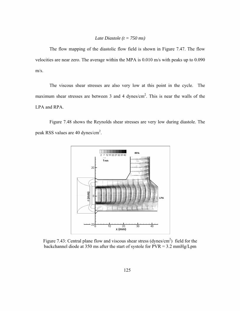
125
Late Diastole (t = 750 ms)
The flow mapping of the diastolic flow field is shown in Figure 7.47. The flow
velocities are near zero. The average within the MPA is 0.010 m/s with peaks up to 0.090
m/s.
The viscous shear stresses are also very low at this point in the cycle. The
maximum shear stresses are between 3 and 4 dynes/cm2. This is near the walls of the
LPA and RPA.
Figure 7.48 shows the Reynolds shear stresses are very low during diastole. The
peak RSS values are 40 dynes/cm2.
Figure 7.43: Central plane flow and viscous shear stress (dynes/cm2) field for the backchannel diode at 350 ms after the start of systole for PVR = 3.2 mmHg/Lpm
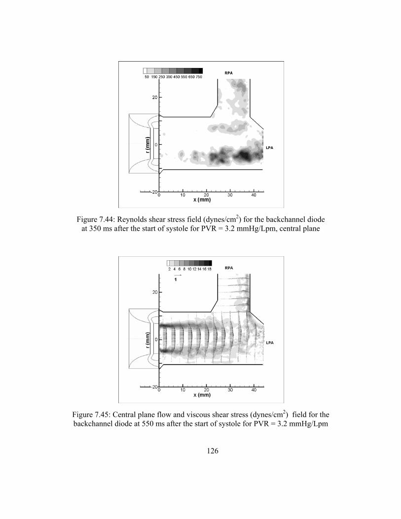
126
Figure 7.45: Central plane flow and viscous shear stress (dynes/cm2) field for the backchannel diode at 550 ms after the start of systole for PVR = 3.2 mmHg/Lpm
Figure 7.44: Reynolds shear stress field (dynes/cm2) for the backchannel diode at 350 ms after the start of systole for PVR = 3.2 mmHg/Lpm, central plane

127
Figure 7.47: Central plane flow and viscous shear stress (dynes/cm2) field for the backchannel diode at 750 ms after the start of systole for PVR = 3.2 mmHg/Lpm
Figure 7.46: Reynolds shear stress field (dynes/cm2) for the backchannel diode at 550 ms after the start of systole for PVR = 3.2 mmHg/Lpm, central plane

128
Case 1 - Offset Plane
The flow profile in the offset plane at 150 ms after the start of systole is in Figure
7.49. The flow exiting the valve is still developing into a core jet. An area of
recirculation occurs within the first 20 mm of the exit. The parabolic profile gives way to
a more uniform profile at this location. The maximum velocity is 0.819 m/s, nearly 4
times the average velocity, 0.184 m/s. The viscous shear stresses are aligned with the
edges of the jet. As the jet ends, the region of shear flares out in the radial direction as
flow reversal takes place. The peak shear stress measures 20 dynes/cm2 at the valve exit.
Figure 7.50 shows the Reynolds shear stresses for the offset plane at t = 150 ms. The
RSS values are low with none measuring higher than 15 dynes/cm2.
Figure 7.48: Reynolds shear stress field (dynes/cm2) for the backchannel diode at 750 ms after the start of systole for PVR = 3.2 mmHg/Lpm, central plane

129
At peak systole the entrained jet is developing over the 22 mm range in Figure
7.51. The peak velocities in the central core jet are 1.493 m/s. The mean axial velocity is
0.311 m/s. The viscous shear stresses can also be seen in Figure 7.51. The peak shear
stresses are along the edges of the jet and measure up to 35 dynes/cm2. The shear layer
flares out as the jet expands downstream. As with the central plane flow, the flow
reattaches to the wall in the lower MPA 15 - 22 mm downstream. There is a resulting
area of wall shear stresses of 9 dynes/cm2. Figure 7.52 shows the RSS measurements at
peak systole. The peak turbulent shear stresses are located 20 mm downstream just
below the centerline. They are about 290 dynes/cm2. The area of mixing occurs closer to
the valve in the lower MPA as it was in the central plane.
The offset plane flow and bulk flow shear stress field is shown in Figure 7.53.
The flow is decelerating and the jet structure is weakening. The peak flow velocities have
slowed to 0.573 m/s and 0.107 m/s on average. The viscous shear stresses peak along the
jet edges at 21 dynes/cm2. There is still a region of higher shear stresses in the lower
MPA where complete flow reversal has occurred. The turbulent shear stress mapping is
in Figure 7.54. The peak turbulent stresses are 175 dynes/cm2. This area is positioned
along the center line about 10 mm downstream.

130
Figure 7.50: Offset Reynolds shear stress (dynes/cm2) field at 150 ms after start of systole for backchannel diode at PVR = 3.2 mmHg/Lpm
Figure 7.49: Offset plane flow and viscous shear stress (dynes/cm2) field at 150 ms after start of systole for backchannel diode at PVR = 3.2 mmHg/Lpm

131
Figure 7.52: Offset Reynolds shear stress (dynes/cm2) field at 350 ms after start of systole for backchannel diode at PVR = 3.2 mmHg/Lpm
Figure 7.51: Offset plane flow and viscous shear stress (dynes/cm2) field at 350 ms after start of systole for backchannel diode at PVR = 3.2 mmHg/Lpm

132
Figure 7.55 maps the flow and viscous shear stresses for the offset plane during
diastole. There is little to no flow at this time in the cardiac cycle. The peak and average
flow velocity are 0.0183 m/s and -0.007 m/s, respectively. The viscous shear stresses are
very low. The difference between the measured shear stresses and the measured noise is
not significant. The turbulent shear stresses are also very low (Figure 7.56). The highest
measured is 10 dynes/cm2.
Figure 7.53: Offset plane flow and viscous shear stress (dynes/cm2) field at 550 ms after start of systole for backchannel diode at PVR = 3.2 mmHg/Lpm

133
Figure 7.55: Offset plane flow and viscous shear stress (dynes/cm2) field at 750 ms after start of systole for backchannel diode at PVR = 3.2 mmHg/Lpm
Figure 7.54: Offset Reynolds shear stress (dynes/cm2) field at 550 ms after start of systole for backchannel diode at PVR = 3.2 mmHg/Lpm

134
Case 3 – Offset Plane
Early Systole (t =150 ms)
The offset flow and viscous shear stress fields (Figure 7.57) are similar to central
plane flow field. The flow profile is uniform and the highest viscous shear stresses are
along the walls. The average and peak velocities are 0.057 m/s and 0.181 m/s,
respectively. The peak wall stresses are about 5 dynes/cm2.
Much of the mixing that occurs 150 ms into the cardiac cycle takes place in the
area downstream of this field of view (where flow is branching off into 2 directions).
Therefore, the RSS measurements are very low in the first 22 mm downstream of the
valve exit as seen in Figure 7.58. The measurements are less than 5 dynes/cm2.
Figure 7.56: Offset Reynolds shear stress (dynes/cm2) field at 750 ms after start of systole for backchannel diode at PVR = 3.2
mmHg/Lpm

135
Peak systole (t = 350 ms)
Figure 7.59 shows the off plane flow and viscous shear stress field during peak
systole. As with the central plane, there is a well defined jet structure. Expectedly, it is
narrower than the central plane jet. The maximum flow speed is 2.07 m/s and the average
is 0.506 m/s. There is an area of recirculation in the below the centerline. The areas of
highest bulk flow shear stresses border the entrained jet. The peak stresses are 55
dynes/cm2 and are just at the valve exit. The wall shear stresses along the lower MPA are
between 10 - 15 dynes/cm2.
The developed area of recirculation in the lower MPA created an area of
turbulence that can be seen in Figure 7.60. At -5 mm below the centerline, there is a
region of elevated turbulent shear stresses. The peak RSS measurements are around 400
dynes/cm2. In general, the Reynolds shear stress values are similar those in the first 22
mm of the central plane data.
Mid diastole (t = 550 ms)
Figure 7.61 is the off plane view of the flow and viscous shear stresses for the mid
diastole phase. The central flow stream is weakening. The maximum and average
velocities have decreased to 0.975 m/s and 0.224 m/s, respectively. The vortical structure
is still present between the jet and the lower wall. There shear layers generated by the
flow separation leads to the peak viscous shear stresses of 23 dynes/cm2 along the edges
of the jet. Figure 7.62 maps the turbulent shear stresses. The higher RSS measurements

136
are positioned in the area of the recirculation where mixing occurs. The peak Reynolds
shear stress is 450 dynes/cm2.
Late Diastole (t = 750 ms)
The diastolic flow profile is shown in Figure 7.63. The average flow velocity is
-0.092 m/s. The peak velocity is -0.213 m/s. The uniform retrograde flow allows for a
complete wash of the artery the walls as it did in the central plane. The wall shear stresses
for this case measure less than 5 dynes/cm2. The overall Reynolds shear stresses during
diastole in the off plane field of view are low (Figure 7.64) at less than 25 dynes/cm2.
Figure 7.57: Offset plane flow and viscous shear stress (dynes/cm2) field at 150 ms after start of systole for backchannel diode at PVR = 5.1 mmHg/Lpm

137
Figure 7.59: Offset plane flow and viscous shear stress (dynes/cm2) field at 350 ms after start of systole for backchannel diode at PVR = 5.1 mmHg/Lpm
Figure 7.58: Offset Reynolds shear stress (dynes/cm2) field at 150 ms after start of systole for backchannel diode at PVR = 5.1 mmHg/Lpm

138
Figure 7.61: Offset plane flow and viscous shear stress (dynes/cm2) field at 550 ms after start of systole for backchannel diode at PVR = 5.1 mmHg/Lpm
Figure 7.60: Offset Reynolds shear stress (dynes/cm2) field at 350 ms after start of systole for backchannel diode at PVR = 5.1 mmHg/Lpm
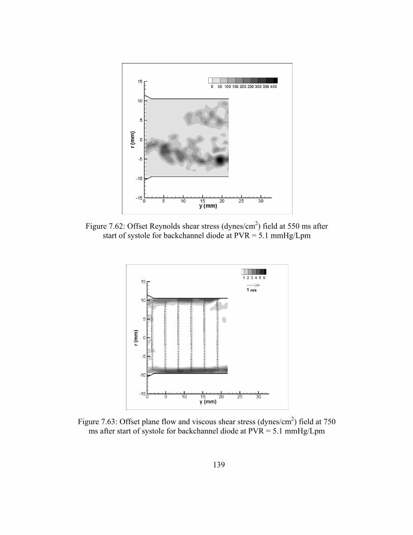
139
Figure 7.63: Offset plane flow and viscous shear stress (dynes/cm2) field at 750 ms after start of systole for backchannel diode at PVR = 5.1 mmHg/Lpm
Figure 7.62: Offset Reynolds shear stress (dynes/cm2) field at 550 ms after start of systole for backchannel diode at PVR = 5.1 mmHg/Lpm

140
Case 4
The final condition under which the backchannel diode was tested was at a PVR =
6.85 mmHg/Lpm and a RF% = 30.5%. The pressure and flow curves are shown in
Figure 7.65.
Early Systole (t = 150 ms)
The velocity and viscous shear stress profile for the diode valve with a
backchannel is mapped in Figure 7.66. The flow is unsettled at this early point in the
cardiac cycle. Flow from the two branches is mixing in the MPA. There is an area of
recirculation that extends from the 5 mm to 22 mm downstream of the valve. The
Figure 7.64: Offset Reynolds shear stress (dynes/cm2) field at 750 ms after start of systole for backchannel diode at PVR = 5.1 mmHg/Lpm

141
average velocity in the MPA was near zero at 0.002 m/s, and the peak velocity was 0.153
m/s.
The resulting viscous shear stresses from this flow field are also shown in Figure
7.66. The measured shear stresses are lower than 5 dynes/cm2. The peak is 4.7 dynes/cm2
along the wall of the upper MPA and the lower LPA.
Figure 7.67 shows the Reynolds shear stresses at 150 ms after the start of the
cycle. The locations of higher RSS are located between 22 and 40 mm downstream
where the flow from the RPA mixes with the flow in the MPA and LPA. Overall, the
RSS values are less than 68 dynes/cm2.
Figure 7.65: Pressure and flow curve for backchannel diode at PVR = 6.9 mmHg/Lpm
-20-10
01020304050607080
0 0.5 1 1.5
mm
Hg,
Lpm
time (s)
Flow Rate RVP PAP

142
Figure 7.67: Reynolds shear stress (dynes/cm2) field for the backchannel diode at 150 ms after the start of systole for PVR = 6.9 mmHg/Lpm
Figure 7.66: Central plane flow and viscous shear stress (dynes/cm2) field for the backchannel diode at 150 ms after the start of systole for
PVR 6.9 mmHg/Lpm

143
Peak Systole (t = 350 ms)
At peak systole, the behavior of the flow is same as it was for the previous cases.
An entrained jet emerges from the valve and travels downstream (Figure 7.68). A higher
flow rate exists, therefore the velocities are higher. There are vortical structures
surrounding the jet. The flow in the RPA is still skewed towards the distal wall, but the
velocity gradient is not as great as it was in cases 2 and 3 for the backchannel diode
(Figure B.39, Figure B.56). The average axial velocity in the main artery is 0.723 m/s.
The peak axial velocity is 2.30 m/s, at the exit of the jet.
The bulk flow shear stresses are also shown in Figure 7.68. Expectedly, the peak
shear stresses are located along the edges of the central jet. The peak shear stress at 350
ms into the cardiac cycle measures 64 dynes/cm2. The wall stresses on the distal RPA
wall range between 19 - 38 dynes/cm2. At the lower wall in the main and into the left
artery branch, the wall stresses are as high as 16 dynes/cm2.
Figure 7.69 shows the turbulent shear stresses for this case at peak systole. The
point of maximum turbulent stresses (1716 dynes/cm2) is in the LPA at the end of the
area of recirculation. Within this same vortical structure, the stresses are around 1000
dynes/cm2. The RSS values reach up to 722 dynes/cm2 where the MPA flow begins to
diverge into the RPA.
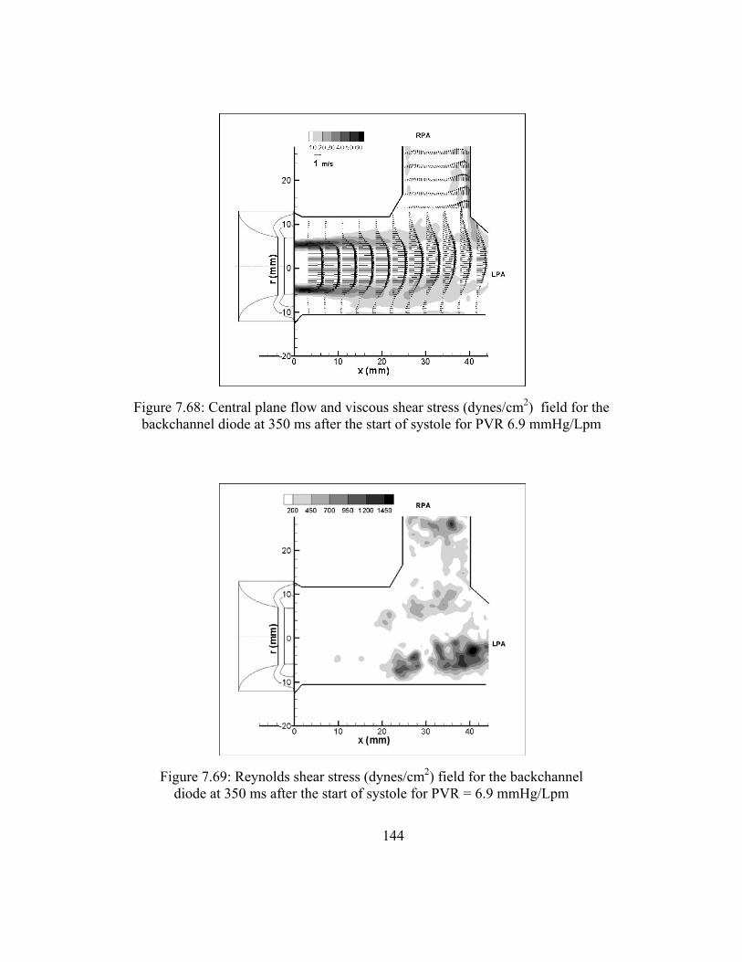
144
Figure 7.69: Reynolds shear stress (dynes/cm2) field for the backchannel diode at 350 ms after the start of systole for PVR = 6.9 mmHg/Lpm
Figure 7.68: Central plane flow and viscous shear stress (dynes/cm2) field for the backchannel diode at 350 ms after the start of systole for PVR 6.9 mmHg/Lpm
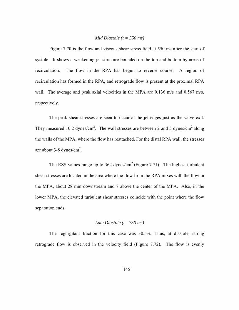
145
Mid Diastole (t = 550 ms)
Figure 7.70 is the flow and viscous shear stress field at 550 ms after the start of
systole. It shows a weakening jet structure bounded on the top and bottom by areas of
recirculation. The flow in the RPA has begun to reverse course. A region of
recirculation has formed in the RPA, and retrograde flow is present at the proximal RPA
wall. The average and peak axial velocities in the MPA are 0.136 m/s and 0.567 m/s,
respectively.
The peak shear stresses are seen to occur at the jet edges just as the valve exit.
They measured 10.2 dynes/cm2. The wall stresses are between 2 and 5 dynes/cm2 along
the walls of the MPA, where the flow has reattached. For the distal RPA wall, the stresses
are about 3-8 dynes/cm2.
The RSS values range up to 362 dynes/cm2 (Figure 7.71). The highest turbulent
shear stresses are located in the area where the flow from the RPA mixes with the flow in
the MPA, about 28 mm downstream and 7 above the center of the MPA. Also, in the
lower MPA, the elevated turbulent shear stresses coincide with the point where the flow
separation ends.
Late Diastole (t =750 ms)
The regurgitant fraction for this case was 30.5%. Thus, at diastole, strong
retrograde flow is observed in the velocity field (Figure 7.72). The flow is evenly

146
distributed in the MPA as well as the branches. The flow speeds have a maximum of -
0.928 m/s and an average of -0.296 m/s.
As a result of the uniform flow profile the wall stresses are higher than within the
flow field. The peak stresses of 12.5 dynes/cm2 during the diastolic phase are seen along
the lower part of the MPA. The right pulmonary artery walls are washed well as the
shear stresses are between 5 and 10 dynes/cm2. Also, stresses of similar magnitude result
from the flow as it is reentering the valve.
Figure 7.73 shows the Reynolds shear stresses that range between 0 and 196
dynes/cm2. The mixing of the two secondary flows creates a higher level of disturbance.
Figure 7.70: Central plane flow and viscous shear stress (dynes/cm2) field for the backchannel diode at 550 ms after the start of systole for PVR 6.9 mmHg/Lpm

147
Figure 7.72: Central plane flow and viscous shear stress (dynes/cm2) field for the backchannel diode at 750 ms after the start of systole for PVR 6.9
mmHg/Lpm
Figure 7.71: Reynolds shear stress (dynes/cm2) field for the backchannel diode at 550 ms after the start of systole for PVR = 6.9 mmHg/Lpm

148
Comparison of Backchannel and Open Cusped Diode Valves
Both valve designs were tested at similar physiological conditions; thus, their
hemodynamic performances can also be compared. In general, the valves had pressure
gradients and regurgitant fractions following the earlier findings; the backchannel diode
valve had lower RF% for some levels of PVR. The most noticeable difference is at for
PVR ~ 4mmHg/Lpm and PVR = 5.1. The backchannel diode experiences RF% levels
that are 50% and 20% lower than that of the open cusped diode valve. Only one data
point was taken at each PVR; therefore, no statistical inference can be about this
comparison.
Figure 7.73: Reynolds shear stress (dynes/cm2) field for the backchannel diode at 750 ms after the start of systole for PVR = 6.9 mmHg/Lpm

149
Table 7.1 summarizes the average and peak velocities, peak viscous shear stresses
and the peak RSS for both valves at PVR = 3 mmHg/Lpm. At the lowest PVR, the
backchannel diode has a more defined jet structure at 150 ms after the start of systole.
The corresponding viscous shear stresses along the edges of the jet are higher for the
backchannel diode than the open cusped. The Reynolds shear stresses are more than 15
times higher for the backchannel at this point as a result of the more active flow. At peak
systole the peak flow speeds are higher for the backchannel diode (1.52 m/s versus 1.28
m/s). All other measurements were similar. As a result, the viscous shear stresses occur
in a similar pattern with higher magnitudes for the backchannel diode. The Reynolds
shear stress fields are similar for each valve as well. During mid diastole and diastole, the
flow behavior for both valves is comparable.
Table 7.1. Comparison PIV Results for Backchannel (PVR = 3.2 mmHg/Lpm) and Open Cusped (PVR = 3.1 mmHg/Lpm) Diode Valves
Open Cusped Diode Backchannel Diode Time (ms)
upeak (m/s)
uavg (m/s)
τ max (d/cm2)
RSSmax (d/cm2)
upeak (m/s)
uavg (m/s)
τ max (d/cm2)
RSSmax (d/cm2)
150 0.150 0.080 3.7 15 0.864 0.260 29.9 225 350 1.280 0.410 32.2 600 1.52 0.445 43.5 735 550 0.600 0.186 12.9 300 0.629 0.163 15 290 750 -0.072 -1.89 4.4 50 0.090 0.010 4 40
As the resistance level increased, the comparison between the open cusped and
backchannel designs did not change much from the first case. The jet flow exiting the

150
backchannel diode valve was more defined at 150 ms after systole start than for the open
cusped diode. The flow for the open cusped valve is still transitioning from retrograde to
antegrade. The maximum RSS for the backchannel valve is almost 3 times higher than
the maximum for the open cusped diode at peak systole (Table 7.2). During diastole,
uniform reverse flow profile is better developed with higher flow speed in the open
cusped diode flow field. This coincides with the higher negative flow rate and RF% that
the open cusped valve experiences.
Table 7.2. Comparison PIV Results for Backchannel (PVR = 4.3 mmHg/Lpm) and Open Cusped (PVR = 4.2 mmHg/Lpm) Diode Valves
Open Cusped Diode Backchannel Diode Time (ms)
upeak (m/s)
uavg (m/s)
τ max (d/cm2)
RSSmax (d/cm2)
upeak (m/s)
uavg (m/s)
τ max (d/cm2)
RSSmax (d/cm2)
150 -0.330 6 78 0.501 0.111 5.0 23 350 1.32 0.504 35 268 1.78 0.517 51.5 800 550 0.824 0.286 17.6 350 0.794 0.228 20.6 540 750 -0.413 -0.149 8.6 60 -0.186 -0.052 4.0 45
For the third PVR level, the flow rate curves generated by the open cusped and
backchannel valves have different shapes. The highest flow rate for the open cusped
diode take places 450 ms after the start of systole instead or 350 ms. During early
systole, the flow for the backchannel diode is fairly uniform antegrade flow while the
flow through the open cusped diode is reversing direction. In fact, the average axial
velocities describe this more aptly. The average velocity for the open cusped design is -
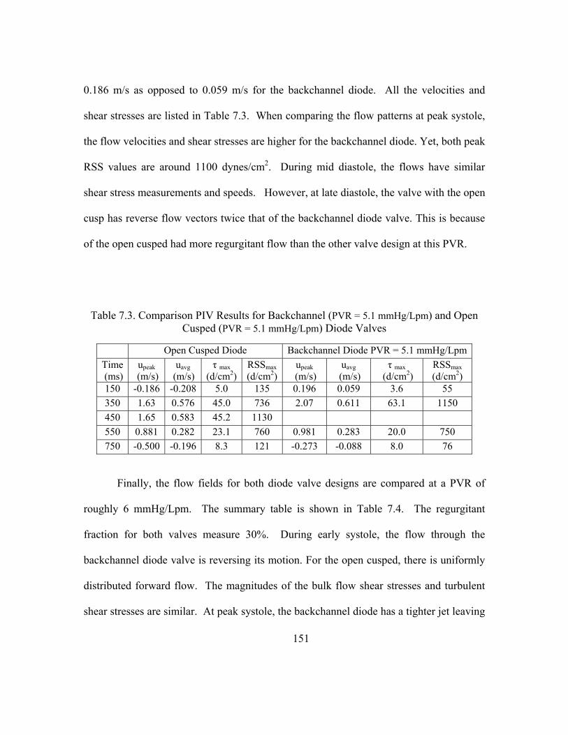
151
0.186 m/s as opposed to 0.059 m/s for the backchannel diode. All the velocities and
shear stresses are listed in Table 7.3. When comparing the flow patterns at peak systole,
the flow velocities and shear stresses are higher for the backchannel diode. Yet, both peak
RSS values are around 1100 dynes/cm2. During mid diastole, the flows have similar
shear stress measurements and speeds. However, at late diastole, the valve with the open
cusp has reverse flow vectors twice that of the backchannel diode valve. This is because
of the open cusped had more regurgitant flow than the other valve design at this PVR.
Table 7.3. Comparison PIV Results for Backchannel (PVR = 5.1 mmHg/Lpm) and Open Cusped (PVR = 5.1 mmHg/Lpm) Diode Valves
Open Cusped Diode Backchannel Diode PVR = 5.1 mmHg/LpmTime (ms)
upeak (m/s)
uavg
(m/s) τ max
(d/cm2)RSSmax (d/cm2)
upeak (m/s)
uavg (m/s)
τ max (d/cm2)
RSSmax (d/cm2)
150 -0.186 -0.208 5.0 135 0.196 0.059 3.6 55 350 1.63 0.576 45.0 736 2.07 0.611 63.1 1150 450 1.65 0.583 45.2 1130 550 0.881 0.282 23.1 760 0.981 0.283 20.0 750 750 -0.500 -0.196 8.3 121 -0.273 -0.088 8.0 76
Finally, the flow fields for both diode valve designs are compared at a PVR of
roughly 6 mmHg/Lpm. The summary table is shown in Table 7.4. The regurgitant
fraction for both valves measure 30%. During early systole, the flow through the
backchannel diode valve is reversing its motion. For the open cusped, there is uniformly
distributed forward flow. The magnitudes of the bulk flow shear stresses and turbulent
shear stresses are similar. At peak systole, the backchannel diode has a tighter jet leaving
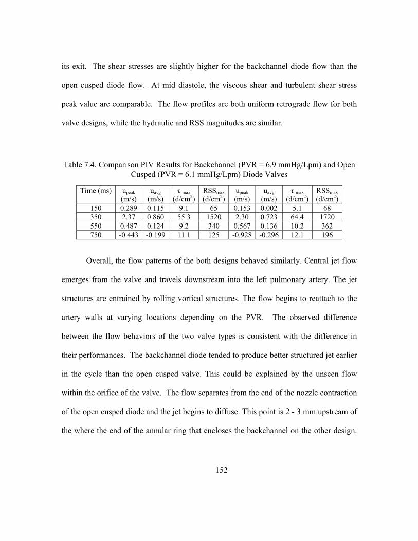
152
its exit. The shear stresses are slightly higher for the backchannel diode flow than the
open cusped diode flow. At mid diastole, the viscous shear and turbulent shear stress
peak value are comparable. The flow profiles are both uniform retrograde flow for both
valve designs, while the hydraulic and RSS magnitudes are similar.
Table 7.4. Comparison PIV Results for Backchannel (PVR = 6.9 mmHg/Lpm) and Open Cusped (PVR = 6.1 mmHg/Lpm) Diode Valves
Time (ms) upeak (m/s)
uavg (m/s)
τ max (d/cm2)
RSSmax (d/cm2)
upeak (m/s)
uavg (m/s)
τ max (d/cm2)
RSSmax (d/cm2)
150 0.289 0.115 9.1 65 0.153 0.002 5.1 68 350 2.37 0.860 55.3 1520 2.30 0.723 64.4 1720 550 0.487 0.124 9.2 340 0.567 0.136 10.2 362 750 -0.443 -0.199 11.1 125 -0.928 -0.296 12.1 196
Overall, the flow patterns of the both designs behaved similarly. Central jet flow
emerges from the valve and travels downstream into the left pulmonary artery. The jet
structures are entrained by rolling vortical structures. The flow begins to reattach to the
artery walls at varying locations depending on the PVR. The observed difference
between the flow behaviors of the two valve types is consistent with the difference in
their performances. The backchannel diode tended to produce better structured jet earlier
in the cycle than the open cusped valve. This could be explained by the unseen flow
within the orifice of the valve. The flow separates from the end of the nozzle contraction
of the open cusped diode and the jet begins to diffuse. This point is 2 - 3 mm upstream of
the where the end of the annular ring that encloses the backchannel on the other design.

153
Thus, the flow field captured with PIV for the open cusped is of a more developed jet
stream.
Shear Stress Level and Exposure Time
Analysis
Various studies suggest that the effect of shear stress on a platelet or erythrocyte
is dependent not only on the magnitude of hat stress, but the amount of time that it is
exposed to this level of stress. The PIV results for both the backchannel and the open
cusped diode valve reveal that the highest levels of the turbulent shear stress occur at
peak systole for the case with the highest PVR. The maximum values were measured in
the area of the shear layer that formed between the jet flow exiting the valve and the
lower wall of the main pulmonary artery.
The total shear was estimated as the sum of the viscous shear stress and the
turbulent shear stress given in equation 19.
(19)
The term most often has the opposite sign of the viscous shear in the same
field; thus, the time average is expected to carry the same sign. Therefore, the total shear
is the difference between the viscous shear and the turbulent shear stresses.
The level of activation as defined by Bluestein et al [55] was found using equation
20.

154
Level of activation = ∑ · ∆ (20)
This level of activation method was calculated in the current study as a means to
estimate the cumulative shear on a particle as it exits a diode valve and travels down the
pulmonary artery.
The highest observed Reynolds shear stress was at the PVR = 6 mmHg/Lpm case
for the backchannel diode during peak systole (t = 350ms). This flow and shear stress
fields are shown in Figure 7.68 and Figure 7.69. The total shear stress for this case is
also the highest. Figure 7.74 shows this the total shear stresses field and three
streamlines within the flow field. The three streamlines were selected as representative of
particle paths that experience high exposure to shear. The first path (identified as 1)
originates at the valve exit and travels along the upper edge of the central core jet, to the
downstream of the MPA and into the RPA near the distal wall. The second streamline
(2) begins at the valve exit and flows downstream into the LPA. This streamline
encounters the region that contains the peak RSS values. The final streamline (3)
originates at the valve exit and travels along the edge of the shear layer in the lower MPA
and LPA. This path also crosses areas with elevated viscous and turbulent shear stresses.
Since pulsatile flow was measured, and data was obtained in time intervals, some
concessions were made in order to estimate the exposure time of a particle. In this case,
the time interval at which data was collected was 50 ms. Therefore, the data collected at

155
350 ms after the start of systole was assumed to be an average representation of the flow
data from t = 325 ms to t = 375 ms.
Results
The markers on the streamlines indicated a particle moving in 1 ms time steps.
The particle along streamlines 1 and 3 are in the flow field for more than 50 ms.
Therefore, the cumulative shear stresses were calculated based on the 50 points that gave
the highest result. The particle in the second path flowed through the field of view in less
than 50 ms since its velocities were of higher magnitudes.
Figure 7.74. Total shear stress field and three streamlines for backchannel diode at PVR = 6.85 mmHg/Lpm 350 ms after the start of systole.
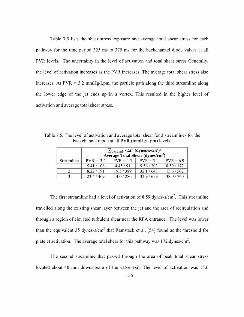
156
Table 7.5 lists the shear stress exposure and average total shear stress for each
pathway for the time period 325 ms to 375 ms for the backchannel diode valves at all
PVR levels. The uncertainty in the level of activation and total shear stress Generally,
the level of activation increases as the PVR increases. The average total shear stress also
increases. At PVR = 3.2 mmHg/Lpm, the particle path along the third streamline along
the lower edge of the jet ends up in a vortex. This resulted in the higher level of
activation and average total shear stress.
Table 7.5. The level of activation and average total shear for 3 streamlines for the backchannel diode at all PVR (mmHg/Lpm) levels.
∑ · ∆ (dynes-s/cm2)/ Average Total Shear (dynes/cm2)
Streamline PVR = 3.2 PVR = 4.3 PVR = 5.1 PVR = 6.9 1 5.41 / 108 4.45 / 91 9.56 / 203 8.59 / 172 2 8.22 / 191 19.5 / 389 32.1 / 643 15.6 / 502 3 23.4 / 469 14.0 / 280 32.9 / 659 38.0 / 760
The first streamline had a level of activation of 8.59 dynes-s/cm2. This streamline
travelled along the existing shear layer between the jet and the area of recirculation and
through a region of elevated turbulent shear near the RPA entrance. The level was lower
than the equivalent 35 dynes-s/cm2 that Ramstack et al. [54] found as the threshold for
platelet activation. The average total shear for this pathway was 172 dynes/cm2.
The second streamline that passed through the area of peak total shear stress
located about 40 mm downstream of the valve exit. The level of activation was 15.6
157
dynes-s/cm2. This path was also subjected to the highest velocities; thus, the particle
displayed through the field in only 31 milliseconds. While this is higher than the
streamline 1 level, it is still less than the threshold for platelet activation. The average
shear stress on this particle was 502 dynes/cm2.
The last streamline began at exit of the valve along the line of flow separation.
This path flows the length of the MPA and into the LPA similar to the second streamline.
The velocity of the particle on this path, however, is lower than that of the second
streamline. As a result, the particle needed 75 ms to travel through the field. Therefore,
the level of activation was based on the 20 - 49th points along the streamline. It was
calculated to be 38.0 dynes-s/cm2. This does pass the threshold established by Ramstack
et al [54], thus, suggesting that at this PVR platelet activation may occur for this case.
LDV Results
The laser Doppler velocimetry data was used to collect flow measurements on a
backchannel flow diode. These measurements were made in accompaniment with the
particle image velocimetry measurements. PIV was used to observe the behavior in the
entire flow field. The PIV data was also used to calculate Reynolds shear and normal
stresses. The LDV methods allow for a higher temporal resolution so that frequency
analysis could be performed.
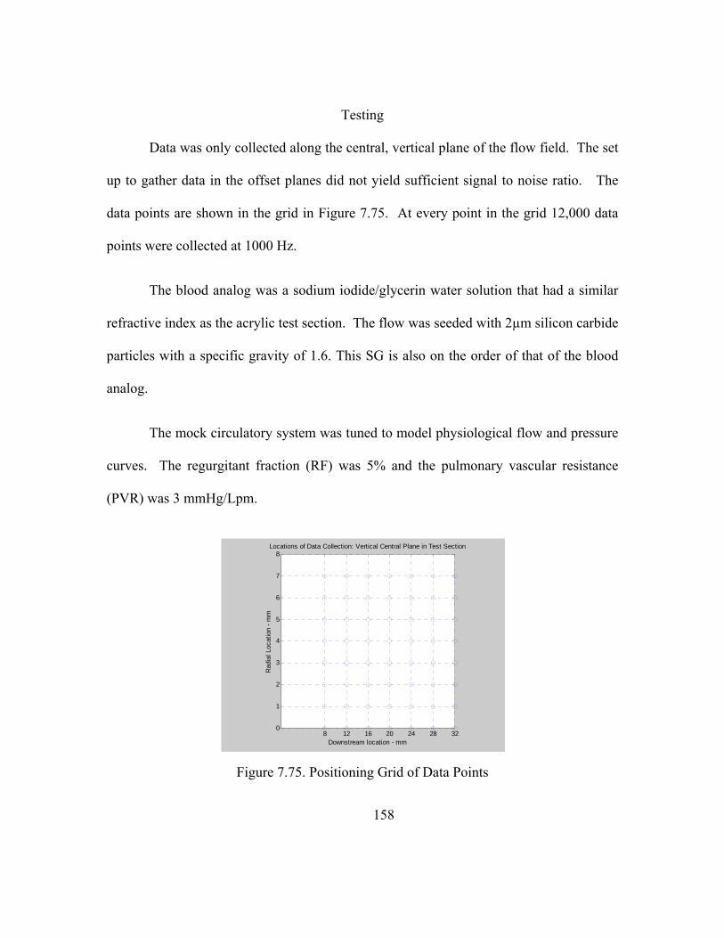
158
Testing
Data was only collected along the central, vertical plane of the flow field. The set
up to gather data in the offset planes did not yield sufficient signal to noise ratio. The
data points are shown in the grid in Figure 7.75. At every point in the grid 12,000 data
points were collected at 1000 Hz.
The blood analog was a sodium iodide/glycerin water solution that had a similar
refractive index as the acrylic test section. The flow was seeded with 2µm silicon carbide
particles with a specific gravity of 1.6. This SG is also on the order of that of the blood
analog.
The mock circulatory system was tuned to model physiological flow and pressure
curves. The regurgitant fraction (RF) was 5% and the pulmonary vascular resistance
(PVR) was 3 mmHg/Lpm.
Figure 7.75. Positioning Grid of Data Points
8 12 16 20 24 28 320
1
2
3
4
5
6
7
8Locations of Data Collection: Vertical Central Plane in Test Section
Downstream location - mm
Rad
ial L
ocat
ion
- mm
159
Post Processing
An algorithm written for Matlab® was used to post process the data. The data
taken at every locale in the grid was saved as a different file containing the 12,000 data
points. The signal was pulsatile, and was therefore made up of many cycles. The mock
circulatory system was pumping at an approximated rate of 75 bpm, or 0.8 Hz. Therefore,
there are up to 15 different cycles taken at every point.
The higher levels of turbulence stress were shown to take place within the shear
layer created by the entrained jet in the PIV results. This was located in the outer 4-5 mm
away from the centerline. The spectral analyses for select points are presented in Figure
7.76 and Figure 7.77.
. The first spectrum for the axial velocity component for a point 28 mm
downstream of the valve and 6 mm above the centerline. Figure 7.76 shows that at the
spectrum of the u’v’, u’2, and v’2. The u’v’ decays at a slope of -1, indicating that large
scale turbulence existed. Above 100 Hz, the slopes drops to -5/3 suggesting that the flow
was beginning to transition from large scale vorticity production to smaller scale eddies.
The u’ and v’ components decay at a slope of -1.
The spectra analysis from further down in the stream (Figure 7.77) shows similar
results. The u’v’ term decays at -1 slope for approximately one decade. At frequencies
above 200 Hz, the slope decreases to -5/3. The u’2 has a similar trend as the -5/3 slope
develops at higher frequencies.

160
Figure 7.76. Spectrum 28 mm Downstream of Backchannel Diode Valve, 6mm above centerline
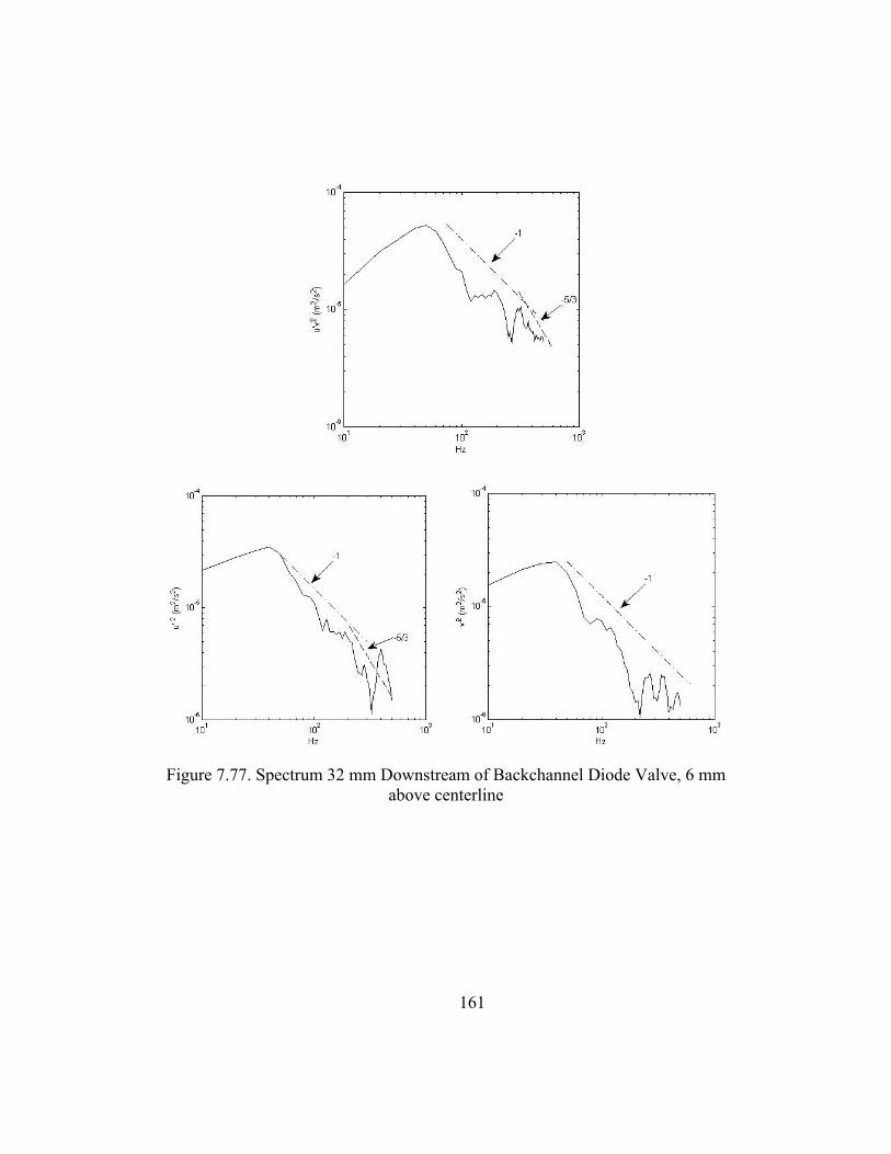
161
Figure 7.77. Spectrum 32 mm Downstream of Backchannel Diode Valve, 6 mm above centerline
162
CHAPTER EIGHT
SUMMARY AND CONCLUSIONS
Summary of Results
Three objectives were posed in this study so as to evaluate momentum diode
valves as pulmonary heart valve replacements. The first objective was to test the
momentum diode valves in vitro over a range of physiological conditions and find the
resulting transvalvular pressure gradients and regurgitant fractions. This was
accomplished with the development of the mock circulatory system that allowed for
testing over a range of physiological conditions. This method was used to then compare
the abilities of the fluid diode valve to regulate flow to that of traditional replacement
valves, such as bileaflet valve and a monoleaflet tilting disk.
In preliminary in vitro studies, the diode valve showed promise as both
regurgitant flow and transvalvular pressure gradients were held to moderate levels for a
range of pulmonary vascular resistances. The diode valve showed improvement in ability
over the flow nozzle to impede regurgitant flow. For a PVR range of 1 to 5 mmHg/lpm,
the diode valve yielded a RF% of 2% to 17% as compared to the 2% to 23% for the
nozzle. Both valves had TVG values up to 17 mmHg. Though these were higher than the
bileaflet and tilting disk valves, RF% and TVG were still within the acceptable range.
Thus, the results of this study support the idea that a motionless momentum diode valve
can be used to regulate flow in the pulmonary position.
163
The acute animal model showed no catastrophic effects of using a motionless
pulmonary valve. An implantation strategy was developed that can be carried into a
chronic test animal model. The in vivo performance results were consistent in both
tendency and magnitude with in vitro findings. In both cases, the RF% and TVG for
normal values of PVC (2 to 3 mL/mmHg) and PVR (2.3 to 3 mmHg/Lpm were within
levels known to be well tolerated in humans. Thus, these findings also suggest that the
diode valve concept can be implemented as a pulmonary heart valve. However, a
compromising factor in these tests was a valve size to patient mismatch, which likely
altered valve flow into the pulmonary artery.
Another objective was to determine the influential geometric parameters on the
valves performance. Each valve design maintained the transvalvular pressure gradient
below 30 mmHg resistance up to 5 mmHg/Lpm. The RF% for all valves was less than
35% for PVR values below 4.5 mmHg/Lpm. At PVR = 2.5 mmHg/Lpm, some designs
had RF% within the 0-20% range. The 60˚ backchannel diode had the lowest RF% and
TVG for some levels of the resistance among the backchannel valves. Conversely, the
60˚ open cusped valve had markedly higher RF% and TVG measurements versus the
other two valves. Therefore, results of this study further lent strength to the hypothesis
that diode valves as replacement pulmonary valves. This study also identified the beta
ratio and interaction between cusp type and the angle of impingement were as tow of the
key parameters affecting the RF% for the diode valves. This information can be used to
conduct further design optimization on the diode valves.
164
A final goal of this study was to use particle image velocimetry (PIV) to study the
hemodynamic performance of different diode designs. The flow fields of both diode
valves showed a jet entrained by areas of recirculation emerging from the valve orifice.
At the highest PVR, the peak velocity through the pulmonary valve in this study were at
times measured to be 2.5 times higher than 0.9 m/s, the average peak velocity in children
[2]. During diastole, the flow was uniformly distributed. The flow speeds for the high
resistance cases peaked at -0.93 m/s. There were slight differences in the flow fields
between the valve types. The backchannel diode featured a better structured jet earlier in
the cycle than the open cusped valve. This could be explained by the unseen flow within
the orifice of the valve.
The PIV studies were conducted in part to determine if the momentum diode
valve would cause shear stresses in the flow to be damaging to the red blood cells or
platelets. The viscous and turbulent shear stresses were always highest during peak
systole. The maximum viscous shear stress values were along the shear layer created by
the jet. For all valves in all cases, the peak viscous shear stresses ranged from 30 and 64
dynes/cm2. The highest turbulent shear stresses were located at the end of a region of
recirculating flow leading into the left pulmonary artery. There were also elevated shear
stresses near the RPA and MPA branch. The highest RSS is 1720 dynes/cm2. The
highest measured shear stress was acquired for the backchannel diode at the highest PVR
during peak systole. The maximum total shear stress was also observed for this case. The
peak level of activation for a particle travelling in the field was found to be 38 dynes-

165
s/cm2. This was 10% higher than the threshold (35 dynes-s/cm2) reported to trigger
platelet activation.
Raised wall shear stress levels were also of concern in this study since they can
result in platelet activation and can trigger eNOS. The distal wall of the RPA was
subjected to highest wall shear stresses at times. At peak systole, the flow into the RPA
was skewed toward the distal wall resulting in shear stresses as high as 30 dynes/cm2.
This was less than the 91 dynes/cm2 reported to cause platelet activation, yet higher than
the 25 dynes/cm2 stated to elevate eNOS.
The regions of recirculation present during peak systole and mid diastole periods,
leaving possibilities for platelet aggregation to take place. The diastolic flow was
uniformly distributed and was shown to sweep the MPA walls with shear stresses
between 3-10 dynes/cm2. This is a good range for wall shear as it is high enough to
effectively wash the walls, but not so high as to trigger platelet activation or release of the
eNOS synthase.
The results from particle image velocimetry revealed that the in many cases, for
levels of regurgitation less than 20%, the flow through the diode valves would not be
expected to have problems with platelet damage, RBC damage or platelet aggregation.
However, in the case with the highest levels of total shear stress, the level of activation
threshold was exceeded and wall shear along the RPA wall was high enough to trigger

166
the release of a vasodilator. So, the diode valve is a plausible solution under certain
physiological conditions.
Conclusions
There are many conclusions that can be taken away from this study. The results of
this study support the original hypothesis with some caveats. First, an experimental
system was developed that was capable of generating physiologically accurate pressure
and flow signals for the pulmonary circulation.
This system was then used to test the conceptual fluid diode in the pulmonary
position and the results of the in vitro tests showed that a fluid diode valve could
acceptably regulate flow the mild levels tolerable in the pulmonary circulation.
The acute in vivo study also showed that the diode valve has promise as a
pulmonary heart valve replacement. The implanted diode was able to regulate flow under
a range of physiological conditions. Moreover, information was gathered on how to
proceed with further animal studies. This information included the preferred surgical
techniques, the need for special implantation tools for the diode valves, the size and
layout of the swine’s heart and pulmonary artery.
The parametric study identified the beta ratio dimension as having a large effect
on the performance of the fluid diode. The cusp enclosure design and the angle of
impingement had varying effects and suggested an interaction of the two dimensions.
This information can be used to further optimize the diode design.
167
Finally, the outcome of the hemodynamic study further supported the hypothesis.
The level of activation was shown to be a function of the pulmonary vascular resistance
and it did not exceed the threshold until the highest level of PVR.
Recommendations
Based on the knowledge of testing methods, diode design and the results from this
the present work, the author has a few recommendation for future work. First, there are a
few suggested changes to the MCS. A ventricle design in which the pressure-volume
curve can be controlled and varied to better simulate the function of the heart should be
implemented. Also the updated ventricle should also be capable of higher heart rates and
stroke volumes so that a wider range of physiological conditions, such as exercise, can be
simulated. The effect of the ventricular – arterial coupling should be studied as it
Since the ability to control the PVR affected the outcome of the parametric
testing, future tests should be carried out using CFD and/or other computational modeling
techniques. The factors will be better controlled; thus, the tests will be able to more
accurately predict the effects of changing geometries.
There are many potential flow studies that can be carried out. The differences
between the backchannel and open cusped diode valves should be studied experimentally
using diodes made of acrylic or other material that will permit for optical studies. In this
way, the flow detail within in the flow channel and cusps of the valves can be seen.
Scaling tests should be conducted in order to find out how smaller diodes compare to the
168
25 mm diodes tested in the current study. Also, the long term effects of the low wall
shear that occurs in the pulmonary artery as a result of the entrained jet should be
explored in order to understand what effect this may have on the vessel walls.
The outcome of the animal model should be taken and applied to future in vivo
tests. The importance of the valve size was emphasized in the animal study. The test
protocol should be expanded to include a better control test. It was shown that an animal
with a healthy heart may not be able to handle the shock of the mild regurgitation and
pressure gradients that are associated with the fluid diode valve. Therefore, an approach
should be developed that takes this into account.

APPENDICES

Appendix A
Multi-Scale Model of the Fluid Diode in the Mock Circulatory System
The lumped parameter model of the mock circulatory system was developed by
Dr. Tim Conover. This appendix contains an excerpt of a report by Conover [122] that
describes the LPM.
Modeling the MCS
Figure A.1 shows the network model to simulate the upstream portion of the MCS
in terms of lumped parameter (zero-dimensional) elements. The source of the blood
analogue fluid is a constant head tank set to provide the systemic venous pressure PSV. A
“big” hose connects the constant head tank to a ball check valve, which simulates the
tricuspid valve of the heart (the action of the right atrium is generally considered
negligible with respect to the pulmonary valve, our area of interest). The model of the
big hose includes quadratic resistance (for both viscous flow and turbulent flow with
Darcy friction factor f=0.02), an exit loss into the constant head tank during reverse flow
only, and inertance. Flow through the big hose is equal to flow through the tricuspid
check valve, QTC.
The ball check valve has a certain range of travel, giving it three effective states,
and it requires a certain amount of reverse flow to close it. In reverse flow, the moment
the ball is seated, shutting the valve, QTC is decelerated to zero impulsively. This is the
closed state. When downstream pressure falls below upstream pressure, the ball opens
and QTC accelerates. In the free state, the ball is assumed to have neutral buoyancy, so it

171
travels with the fluid, and it adds no resistance to the flow. The ball’s position is
represented by the volume of fluid that sweeps it along, VBV, which is the time-integral of
QTC. The ball strikes a pin limiting its forward travel, setting the pinned state. The
minimum value of VBV to strike the pin, according to the geometry of the ball valve
chamber, is 10.2 ml. In the pinned state the fluid must accelerate through the annular gap
between the ball and the cylindrical walls of its chamber, causing a pressure drop in the
manner of an orifice. When QTC reverses the ball moves freely again, backwards, until it
closes.
Flow through the ball valve enters the ventricle chamber, in which the flow is
confined in a concentric respirator bag, similar to the construction of the pulmonary
compliance chambers. Both the elasticity of the bag and the compressibility of air
Figure A.1. Lumped parameter model for the upstream of the Mock Circulatory System.
+PSV
Rbig Lbig
QTC "Tricuspid" ball check valve
Cbag
CRV
PVC
VH
Harvard Pump Cylinder
Ventricle Chamber
QVH
RVH LVH
Cb
RVP
Q
Diode Inlet
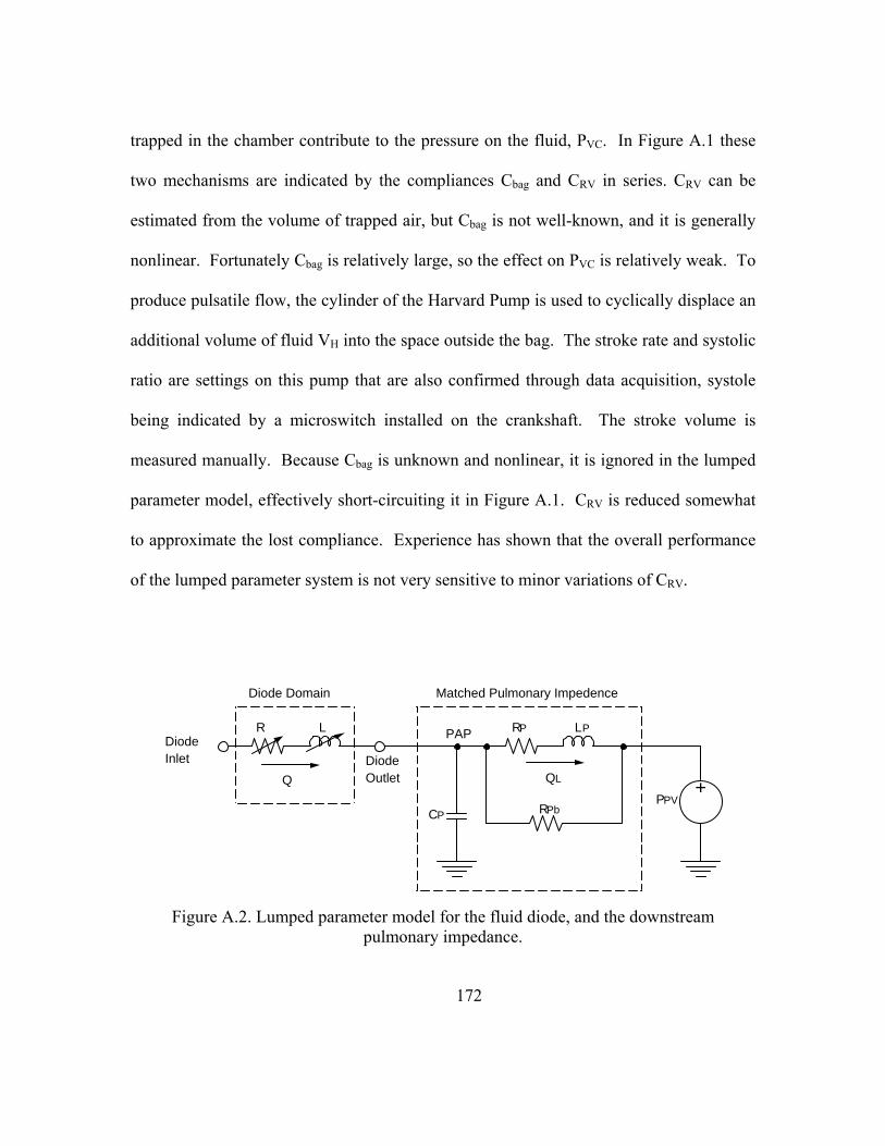
172
trapped in the chamber contribute to the pressure on the fluid, PVC. In Figure A.1 these
two mechanisms are indicated by the compliances Cbag and CRV in series. CRV can be
estimated from the volume of trapped air, but Cbag is not well-known, and it is generally
nonlinear. Fortunately Cbag is relatively large, so the effect on PVC is relatively weak. To
produce pulsatile flow, the cylinder of the Harvard Pump is used to cyclically displace an
additional volume of fluid VH into the space outside the bag. The stroke rate and systolic
ratio are settings on this pump that are also confirmed through data acquisition, systole
being indicated by a microswitch installed on the crankshaft. The stroke volume is
measured manually. Because Cbag is unknown and nonlinear, it is ignored in the lumped
parameter model, effectively short-circuiting it in Figure A.1. CRV is reduced somewhat
to approximate the lost compliance. Experience has shown that the overall performance
of the lumped parameter system is not very sensitive to minor variations of CRV.
Figure A.2. Lumped parameter model for the fluid diode, and the downstream pulmonary impedance.
Diode Inlet
Q
R L
Diode Outlet
CP
PAP
Diode Domain
QL
RP LP
RPb
+PPV
Matched Pulmonary Impedence

173
The flow out of the ventricle chamber and through the hose to the test section is
QVH. The hose is modeled with a quadratic resistance (with the turbulent friction
increased to f=0.06 to accommodate the several barbs in this hose), an exit loss into the
test section during forward flow only, and an inertance. Finally, Figure A.1 shows a
buffer compliance element with compliance Cb, operating at the Right Ventricular
Pressure (RVP). This small-value compliance does not represent any perceptible
compliance in the real test section, but it is necessary to stabilize the numerical model.
The RVP sets the inlet boundary of the model in Fluent, and it represents the RVP which
is measured in the real test section.
Figure A.1 shows the lumped parameter model of the “diode,” which is actually
the whole test section, and the pulmonary impedance. The flow rate through the diode is
Q. The pressure-flow characteristics of the fluid diode can be approximated by a
nonlinear quadratic resistance and a nonlinear inertance in series, a total of six
parameters. This model is accurate enough for design of experiment work, and for
setting up initial conditions for the multi-scale model in Fluent. Naturally the six-
parameter model is not part of the model in Fluent.
There was a considerable effort made to model the actual physics of the
downstream section of the MCS in terms of lumped parameters. Unfortunately the
concentric compliance chambers are complex, nonlinear, continuous systems, and the
modeling results were not good. Alternatively, for a given experimental case, a linear
systems technique can be used to identify a non-unique system of linear components
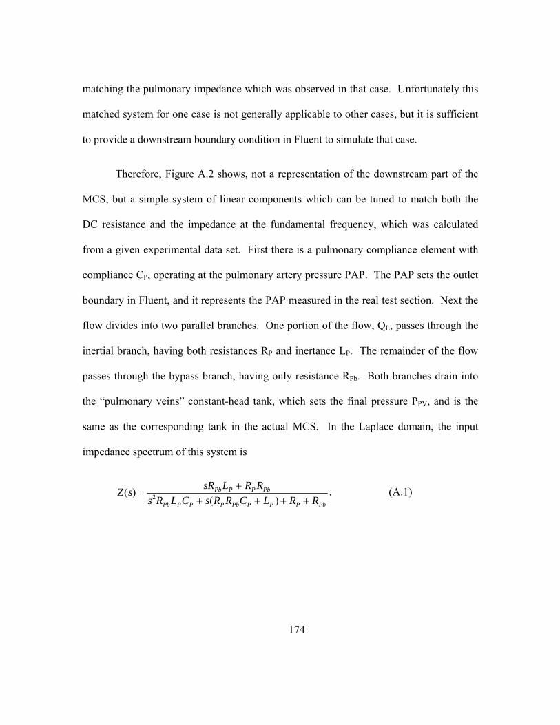
174
matching the pulmonary impedance which was observed in that case. Unfortunately this
matched system for one case is not generally applicable to other cases, but it is sufficient
to provide a downstream boundary condition in Fluent to simulate that case.
Therefore, Figure A.2 shows, not a representation of the downstream part of the
MCS, but a simple system of linear components which can be tuned to match both the
DC resistance and the impedance at the fundamental frequency, which was calculated
from a given experimental data set. First there is a pulmonary compliance element with
compliance CP, operating at the pulmonary artery pressure PAP. The PAP sets the outlet
boundary in Fluent, and it represents the PAP measured in the real test section. Next the
flow divides into two parallel branches. One portion of the flow, QL, passes through the
inertial branch, having both resistances RP and inertance LP. The remainder of the flow
passes through the bypass branch, having only resistance RPb. Both branches drain into
the “pulmonary veins” constant-head tank, which sets the final pressure PPV, and is the
same as the corresponding tank in the actual MCS. In the Laplace domain, the input
impedance spectrum of this system is
Z(s) = sRPbLP + RP RPb
s2RPbLPCP + s(RP RPbCP + LP ) + RP + RPb
. (A.1)

175
Results from Lumped Parameter Model Tests
Table A.1 shows all the results from the LPM using different upstream inertance
values. The inertance level for the system as it was originally calibrated was 8.79E-3
mmHg-s2/mL. When the inertance was 3.4E-2 mmHg-s2/mL, there was minimal
backflow.
Table A.1. Results from LPM Tests
Lvh (mmHg-s2/mL)
CO (Lpm)
RF % PVR (mmHg/Lpm)
PVC (mL/mmHg)
TVG (mmHg)
8.79E-03 5.3 11.1 3.1 2.9 6.9 4.00E-03 5.1 11.7 3.2 2.7 7.9 2.00E-03 5.1 11.8 3.2 2.7 8.1 1.00E-03 5.1 11.7 3.2 2.7 8.6 1.50E-02 5.7 8.6 3.0 3.2 6.5 3.00E-02 7.5 1.09 2.6 4.0 9.5 3.40E-02 7.8 0.08 2.6 4.3 9.7 6.00E-02 9.9 0.0 2.3 6.5 11.4
176
APPENDIX B
PIV Results
Open Cusped Diode - Case 2
The pressure and flow curve for the moderate PVR and RF% case is shown in
Figure B.1. The flow rates range from 14 Lpm to – 3.5 Lpm. The PVR = 4.3
mmHg/Lpm. The regurgitant fraction for this setting is 12.4%.
Early systole (t = 150 ms)
Figure B.2 shows the flow and viscous shear stress fields at the PVR = 4.3
mmHg/Lpm case 150 ms into the cycle. The average velocity in the MPA at this time in
the cycle is -0.0333 m/s. the peak velocity is – 0.17 m/s. Noticeable reverse flow from
the LPA reenters the MPA and an area of recirculation is formed in the lower radial part
of the main artery. Also, the flow from the RPA rejoins the flow in the MPA and
impinges upon the retrograde jet from the LPA. On the upper main artery wall, there is
another region of recirculation between the regions of retrograde flow and antegrade
flow.
The measured viscous stresses are very low; they are less than 6 dynes/cm2. The
highest bulk flow stresses at this point occur along the shear layer resulting from the flow
from the LPA and RPAs mixing shown in Figure B.2.
The peak turbulent shear stresses during early systole are on the order of 50
dynes/cm2 (Figure B.3). This coincides with region where the branch flows collide and

177
where the shear layers exist (Figure B.2). The peak turbulent stresses 150 ms for the Case
2 are 2 – 3 times higher than Case 1 (PVR = 3.1 mmHg/Lpm) likely because of a higher
rate of mixing there.
Peak Systole (t = 350 ms)
At peak systole, a central jet structure is discernible (Figure B.4). There is an area
of recirculation along the lower radii of the MPA, that reattaches before the entering the
LPA. Moreover, unlike the PVR = 3.1 mmHg/Lpm case, there is no recirculation in the
RPA branch. Instead, the flow follows the RPA bend well. Therefore, the secondary flow
in both branches is well formed. The flow once again impinges the artery wall at the
bifurcation. The peak velocities are 1.32 m/s and the average MPA velocity is now 0.504
m/s.
As the cycle progresses, and peak systole is reached (t = 350 ms) the peak viscous
shear stresses are about 35 dynes/cm2 (Figure B.4). They occur along the edges of the
entrained jet structure. The magnitudes are similar to those observed in Case 1. The
primary flow branches into the RPA rather smoothly and this results in well defined flow
into RPA. Thus, there are measureable wall shear stresses along the distal RPA wall.
Additionally, there is a shear layer present between the proximal RPA wall and the jet
flow into the RPA.
Figure B.5 shows the Reynolds shears stresses field at t = 350 ms after the start of
systole. The turbulence levels are less in this case than at PVR = 3.1 mmHg/Lpm.

178
(Figure 7.7). At the lowest PVR, the flow field had an area of recirculation that created
mixing near the RPA and MPA and between the LPA and MPA. For PVR = 4.3
mmHg/Lpm, the flow transitions more smoothly into the RPA as shown in Figure B.4.
One of the locations where peak turbulent shear stresses occur is in the 90º turn in the
RPA where flow separation occurs. Also, RSS levels are 200-300 dynes/cm2 along both
walls of the main artery and at the inner RPA wall within the shear layer that exists.
Mid Diastole (t = 550 ms)
As the flow decelerates, the jet structure is still present (Figure B.6). There are
noticeable shear layers between the regions of antegrade and retrograde flow in the upper
and lower radial locations of the main pulmonary artery. At this point in the cycle an
area of recirculation is now seen in the RPA entrance; thus, resulting in an area of stasis.
The peak and average MPA velocities are 0.824 m/s and 0.286 m/s, respectively.
The peak shear stress values at 550 ms after the start of systole are about 14
dynes/cm2 (Figure B.6). This is comparable to the 1st case. These areas of higher shear
are along the edges of the jet structure, at the distal RPA wall, and between the antegrade
flow and the lower MPA wall.
Figure B.7 show the turbulent shear stress field 550 ms after the start of systole
for PVR = 4.3 mmHg/Lpm. The turbulent shear stresses are high at the edge of the
combining flow of the RPA and MPA (Figure B.6). Also, some of the highest levels take

179
place where the flow separation occurs in the LPA. This is similar to the PVR = 3.1
mmHg/Lpm case during mid diastole.
Late Diastole (t = 750 ms)
The diastolic flows plotted in Figure B.8: shows well defined, undisturbed
retrograde flow in the MPA and the branches. There is a small area of stasis near the
branch between the left and right branches. Otherwise, the flow is sufficient to promote
wall shear stresses needed to wash the artery wall. The peak velocities are -0.413 m/s
and the average velocity is similarly -0.149 m/s.
The peak shear stresses of 10 dynes/cm2. These are along the lower MPA and
LPA walls where the most noticeable retrograde flow existed. At the other walls the
shear was one half of the peak.
The turbulent shear stresses during diastole are shown in Figure B.9. The values
are less than 40 dynes/cm2 everywhere except where the retrograde flows from the left
and right arteries meet. The RSS values for PVR = 4.3 mmHg/Lpm are double of that for
PVR = 3.1 mmHg/Lpm.
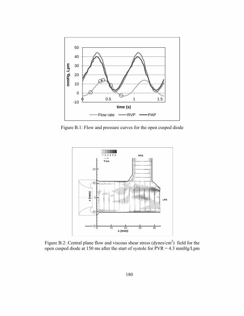
180
Figure B.2: Central plane flow and viscous shear stress (dynes/cm2) field for the open cusped diode at 150 ms after the start of systole for PVR = 4.3 mmHg/Lpm
Figure B.1: Flow and pressure curves for the open cusped diode
-10
0
10
20
30
40
50
0 0.5 1 1.5
mm
Hg,
Lpm
time (s)
Flow rate RVP PAP

181
Figure B.4: Central plane flow and viscous shear stress (dynes/cm2) field for the open cusped diode at 350 ms after the start of systole for PVR = 4.3 mmHg/Lpm
Figure B.3: Reynolds shear stress field (dynes/cm2) for the open cusped diode at 150 ms after the start of systole for PVR = 4.3 mmHg/Lpm, central plane

182
Figure B.6: Central plane flow and viscous shear stress (dynes/cm2) field for the open cusped diode at 550 ms after the start of systole for PVR = 4.3 mmHg/Lpm
Figure B.5: Reynolds shear stress field (dynes/cm2) for the open cusped diode at 350 ms after the start of systole for PVR = 4.3 mmHg/Lpm, central plane

183
Figure B.8: Central plane flow and viscous shear stress (dynes/cm2) field for the open cusped diode at 750 ms after the start of systole for PVR = 4.3 mmHg/Lpm
Figure B.7: Reynolds shear stress field (dynes/cm2) for the open cusped diode at 550 ms after the start of systole for PVR = 4.3 mmHg/Lpm, central plane

184
Open Cusped Diode Case 2 - Offset Planes
Figure B.10 shows the offset plane flow and viscous shear stress for the moderate
PVR and RF% case at 150 ms after the start of systole. The flow profile is uniform. The
average axial flow is -0.044 m/s, and the peak velocity is -0.170 m/s. The viscous shear
stresses are highest near the walls. The peak value is between 3-4 dynes/cm2. The
Reynolds shear stress field is in Figure B.11. There is little disturbance in the MPA
within 22 mm of the valve exit. The peak RSS values reach up to 25 dynes/cm2.
At peak systole the velocity profile is parabolic (Figure B.12). A jet structure is
evident just as it was in the central plane. The average axial velocity is 0.422 m/s. The
peak velocity is 1.27 m/s. The bulk flow shear stresses are up to 25 dynes/cm2 just as the
jet forms at the valve exit. The wall shear stresses are up to 4 dynes/cm2 where the flow
has reattached to the artery wall. The offset plane Reynolds shear stresses at peak systole
are shown in Figure B.13. The high regions are near the areas of recirculation 6 mm
away from the centerline with maximum values of RSS up to 250 dynes/cm2.
The offset plane flow and viscous shear stresses during deceleration at PVR =
4.25 Wood’s unit are in Figure B.14. The peak axial velocity is 0.693 m/s. The average
velocity is 0.207 m/s. The peak hydraulic shear stresses are 14 dynes/cm2. The peak
RSS values are on the order of 150 dynes/cm2, lower than at peak systole (Figure B.15).
The higher regions of turbulence shear stress take place in the areas of recirculation.
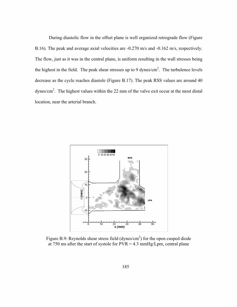
185
During diastolic flow in the offset plane is well organized retrograde flow (Figure
B.16). The peak and average axial velocities are -0.270 m/s and -0.162 m/s, respectively.
The flow, just as it was in the central plane, is uniform resulting in the wall stresses being
the highest in the field. The peak shear stresses up to 9 dynes/cm2. The turbulence levels
decrease as the cycle reaches diastole (Figure B.17). The peak RSS values are around 40
dynes/cm2. The highest values within the 22 mm of the valve exit occur at the most distal
location, near the arterial branch.
Figure B.9: Reynolds shear stress field (dynes/cm2) for the open cusped diode at 750 ms after the start of systole for PVR = 4.3 mmHg/Lpm, central plane
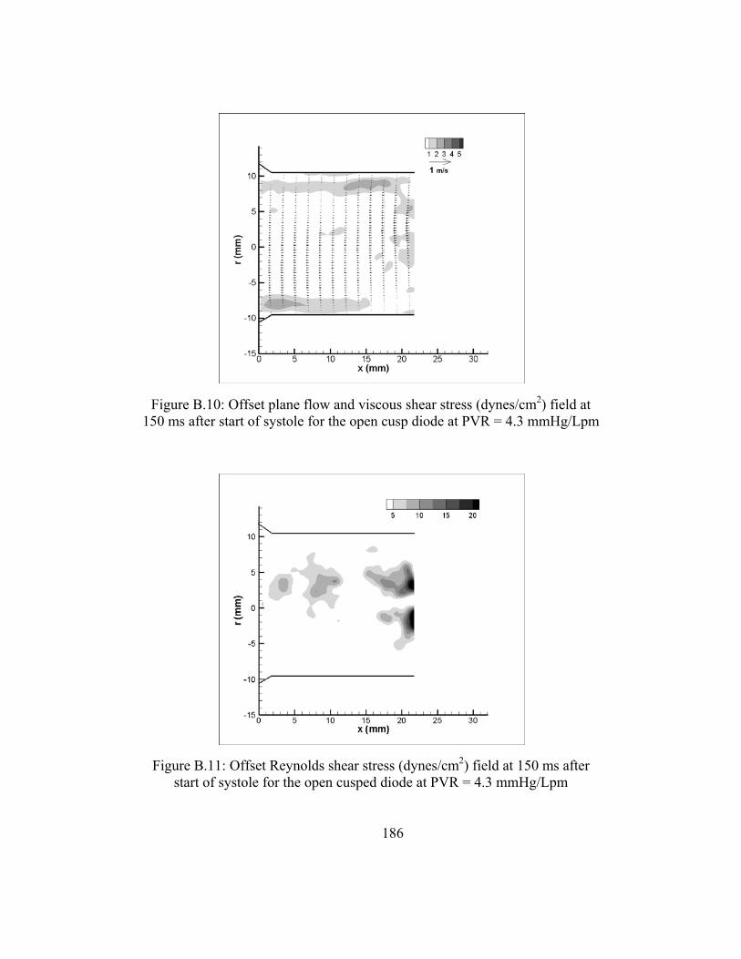
186
Figure B.11: Offset Reynolds shear stress (dynes/cm2) field at 150 ms after start of systole for the open cusped diode at PVR = 4.3 mmHg/Lpm
Figure B.10: Offset plane flow and viscous shear stress (dynes/cm2) field at 150 ms after start of systole for the open cusp diode at PVR = 4.3 mmHg/Lpm

187
Figure B.13: Offset Reynolds shear stress (dynes/cm2) field at 350 ms after start of systole for the open cusped diode at PVR = 4.3 mmHg/Lpm
Figure B.12: Offset plane flow and viscous shear stress (dynes/cm2) field at 350 ms after start of systole for the open cusp diode at PVR = 4.3 mmHg/Lpm

188
Figure B.15: Offset Reynolds shear stress (dynes/cm2) field at 550 ms after start of systole for the open cusped diode at PVR = 4.3 mmHg/Lpm
Figure B.14: Offset plane flow and viscous shear stress (dynes/cm2) field at 550 ms after start of systole for the open cusp diode at PVR = 4.3 mmHg/Lpm

189
Figure B.17: Offset Reynolds shear stress (dynes/cm2) field at 750 ms after start of systole for the open cusped diode at PVR = 4.3 mmHg/Lpm
Figure B.16: Offset plane flow and viscous shear stress (dynes/cm2) field at 750 ms after start of systole for the open cusp diode at PVR = 4.3 mmHg/Lpm

190
Open Cusped Diode Case 3 – Offset Planes
Early Systole (t= 150 ms)
The velocity and viscous shear stress profile for the offset plane at t = 150 ms is
shown in Figure B.18. The flow is uniform and diminishing at the walls. Therefore, the
shear stresses are highest at the walls. The peak viscous shear stress is less than 5
dynes/cm2. The average velocity is -0.0056 m/s in the main pulmonary artery with peaks
up to -0.202 m/s. Figure B.19 is the Reynolds shear stress field 150 ms after the start of
the cardiac cycle. The turbulent stresses range up to 40 dynes/cm2. The peak RSS occur
on the centerline approximately 20 mm downstream.
Figure B.18: Offset plane flow and viscous shear stress (dynes/cm2) field for the open cusped diode at 150 ms after start of systole at PVR = 5.1 mmHg/Lpm

191
Systole (t = 350 ms)
The offset plane flow and viscous shear stress field during systole shows a
developing jet structure (Figure B.20). The areas of recirculation are seen 5 mm from the
centerline. The flow reattaches to the wall in the lower MPA. The peak velocity is 1.64
m/s and averaged 0.463 m/s. The peak viscous shear stresses are along the edges of the
jet. The highest shear values are seen just at the valve exit at 42 dynes/cm2. The wall
shear stresses are measured at 4 dynes/cm2 at the upper MPA wall and 9 dynes/cm2 at the
lower wall. Figure B.21 shows the turbulent shear stress field at 350 ms after the start of
systole. The highest RSS values are 42 dynes/cm2.
Figure B.19: Offset Reynolds shear stress (dynes/cm2) field for the open cusped diode at 150 ms after start at PVR = 5.1 mmHg/Lpm
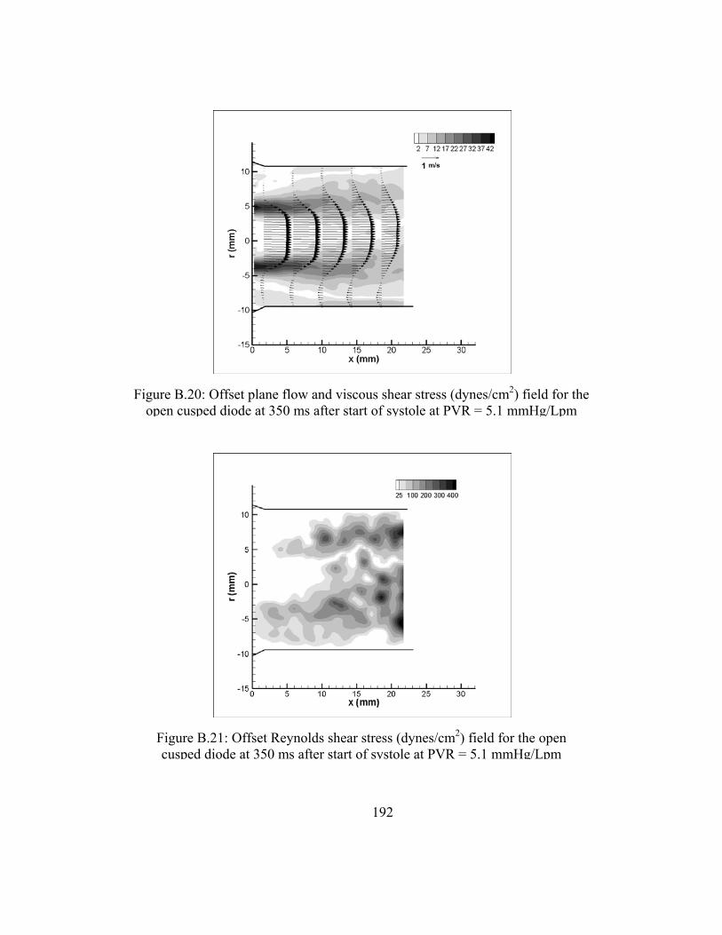
192
Figure B.21: Offset Reynolds shear stress (dynes/cm2) field for the open cusped diode at 350 ms after start of systole at PVR = 5.1 mmHg/Lpm
Figure B.20: Offset plane flow and viscous shear stress (dynes/cm2) field for the open cusped diode at 350 ms after start of systole at PVR = 5.1 mmHg/Lpm

193
Peak systole (t = 450 ms)
The peak flow rate occurs at 450 ms after the start of systole. The offset plane
flow and shear stresses fields are shown in Figure B.22. The jet structure is well
developed. The maximum axial velocity is lower than at 350 ms, at 1.60 m/s, and the
average is 0.463 m/s. The peak viscous shear stresses along the edges of the jet are 35
dynes/cm2. This is also lower than at 350 ms. The reverse flow is of a lower magnitude at
the upper MPA than at the lower wall. Therefore, the wall shear stresses are less than 3
dynes/cm2 at the upper wall and as high as 8 dynes/cm2. The highest turbulent shear
stresses at peak systole were observed in the areas of recirculation (Figure B.23). The
RSS values peak at 350 dynes/cm2.
Figure B.22: Offset plane flow and viscous shear stress (dynes/cm2) field for the open cusped diode at 450 ms after start of systole at PVR = 5.1 mmHg/Lpm

194
Mid Diastole (t = 550 ms)
Figure B.24 shows the velocity profile during the mid diastole phase of the cycle.
The velocities have lessened and the profile has flattened out. The average is 0.79 ms/
and the peak is 1.0 m/s. The shearing rate is also lower; the peak viscous shear stresses
are only 13 dynes/cm2. The wall shear stresses are less than 6 dynes/cm2. The turbulent
shear stress levels are similar to that observed at peak systole (Figure B.25). The field
nearer the upper MPA wall has turbulence levels up to 235 dynes/cm2 and the area in the
lower radial position has RSS values as high as 350 dynes/cm2.
Figure B.23: Offset Reynolds shear stress (dynes/cm2) field for the open cusped diode at 450 ms after start of systole at PVR = 5.1 mmHg/Lpm

195
Figure B.25: Offset Reynolds shear stress (dynes/cm2) field for the open cusped diode at 550 ms after start of systole at PVR = 5.1 mmHg/Lpm
Figure B.24: Offset plane flow and viscous shear stress (dynes/cm2) field for the open cusped diode at 550 ms after start of systole at PVR = 5.1 mmHg/Lpm

196
Late Diastole (t = 750 ms)
Strong retrograde flow is present during diastole as seen in Figure B.26. The flow
is like that in the central plane. It is uniform. The peak velocity is 0.358 m/s and the
average velocity is 0.214 m/s. The highest shear stresses are about 10 dynes/cm2 and
occur along the walls. At this point in the cycle, the Reynolds shear stresses measure less
than 50 dynes/cm2.
Figure B.26: Offset plane flow and viscous shear stress (dynes/cm2) field for the open cusped diode at 750 ms after start of systole at PVR = 5.1 mmHg/Lpm

197
Open Cusped Diode Case 4 – Offset Plane
Early Systole (t = 150 ms)
The offset flow plane for the open cusped diode is shown in Figure B.28. The
flow field presented for this plane is only in the main pulmonary artery. The flow at 150
ms after systole start is uniformly distributed. The average axial velocity is 0.103 m/s.
The peak velocity is 0.379 m/s. The peak shear stress is 8.7 dynes/cm2. The Reynolds
shear stresses within the first 22 mm of the valve exit are low, as the highest turbulence
shear stress levels occur in the area of the artery branch (Figure B.29).
Figure B.27: Offset Reynolds shear stress (dynes/cm2) field for the open cusped diode at 750 ms after start of systole at PVR = 5.1 mmHg/Lpm

198
Figure B.29: Offset Reynolds shear stress (dynes/cm2) field for the open cusped diode at 150 ms after start of systole for open cusped diode at PVR =
6.1 mmHg/Lpm
Figure B.28: Offset plane flow and viscous shear stress (dynes/cm2) field for the open cusped diode at 150 ms after the start of systole for PVR 6.1 mmHg/Lpm

199
Peak Systole (t = 350 ms)
At peak systole, a narrower jet structure is seen in the offset flow plane than in the
central plane (Figure B.30). The jet flow is entrained by two recirculating regions. The
peak velocity was measured at 1.8 m/s and the average velocity is 0.313 m/s. The viscous
shear stress field is also seen in Figure B.30. Viscous shear stresses of 31 dynes/cm2 are
at the edges of the entrained jet. The Reynolds shear stresses peak at 857 dynes/cm2
(Figure B.31) and occur within the vortices.
Mid Diastole (t = 550 ms)
During mid diastole the flow behaves in the off center flow plane is comparable to
that in the central plane. The flow velocities have decelerated to an average velocity of
0.019 m/s with peak velocity values of 0.221 m/s. The shear stresses are low. The
maximum values of hydraulic shear are throughout the field. There are three discernible
shear layers observed between the diminishing jet and the retrograde flow near the walls.
The peak viscous stresses are 5.1 dynes/cm2. Figure B.33 shows that the RSS values
reach a maximum at 242 dynes/cm2.
Diastole (t =750 ms)
As was the case with the central plane, the diastolic flow in the off center plane
has a uniform profile Figure B.34. Retrograde flow is predominant; thus, the average
axial velocity is -0.090 m/s and it peaks at -0.416 m/s. Since the flow is evenly
distributed across the offset plane cross section, the flow provides a sweeping of the

200
aretery walls. The peak viscous shear stresses are 7.5 dynes/cm2 along the walls. The
Reynolds shear stresses are just as low at 39 dynes/cm2 (Figure B.35).
Backchannel Diode - Case 2
The pressure and flow curves for the moderate PVR and RF% case for the back -
channel diode are shown in Figure B.36. The PVR = 4.1 mmHg/Lpm and the RF% =
6.25. The flow rate spans from 14 Lpm to – 2.1 Lpm.
Early Systole (t =150 ms)
The central plane flow and viscous shear stress field for 150 ms after the start of
systole is in Figure B.37. A jet formation present at the valve exit; however, by 10 mm
downstream the axial flow profile in the MPA is uniform. The average is 0.111 m/s and
the peak velocity is 0.501 m/s. The flow velocities in the left and right branches are
uniformly distributed.
The shear stresses in the shear layer created by the emerging jet measure up to 11
dynes/cm2 (Figure B.37). This is observed within the first 10 mm of the valve exit. As
the flow reattaches to the wall, the shear stresses reach 5 dynes/cm2 in the lower MPA
and LPA, and 6 dynes/cm2 in the upper MPA. There is a flow gradient along the distal
RPA wall that generates shear stress 4 - 5 dynes/cm2.
The Reynolds shear stresses are mapped in Figure B.38. They peak at 23
dynes/cm2. The maximum turbulent stresses are located where the recirculation ends.

201
Figure B.31: Offset Reynolds shear stress (dynes/cm2) field for the open cusped diode at 350 ms after start of systole for open cusped diode at PVR = 6.1
mmHg/Lpm
Figure B.30: Offset plane flow and viscous shear stress (dynes/cm2) field for the open cusped diode at 350 ms after the start of systole for PVR 6.1 mmHg/Lpm

202
Figure B.33: Offset Reynolds shear stress (dynes/cm2) field for the open cusped diode at 550 ms after start of systole for open cusped diode at PVR = 6.1
mmHg/Lpm
Figure B.32: Offset plane flow and viscous shear stress (dynes/cm2) field for the open cusped diode at 550 ms after the start of systole for PVR 6.1 mmHg/Lpm

203
Figure B.35: Offset Reynolds shear stress (dynes/cm2) field for the open cusped diode at 750 ms after start of systole for open cusped diode at PVR =
6.1 mmHg/Lpm
Figure B.34: Offset plane flow and viscous shear stress (dynes/cm2) field for the open cusped diode at 750 ms after the start of systole for PVR 6.1
mmHg/Lpm
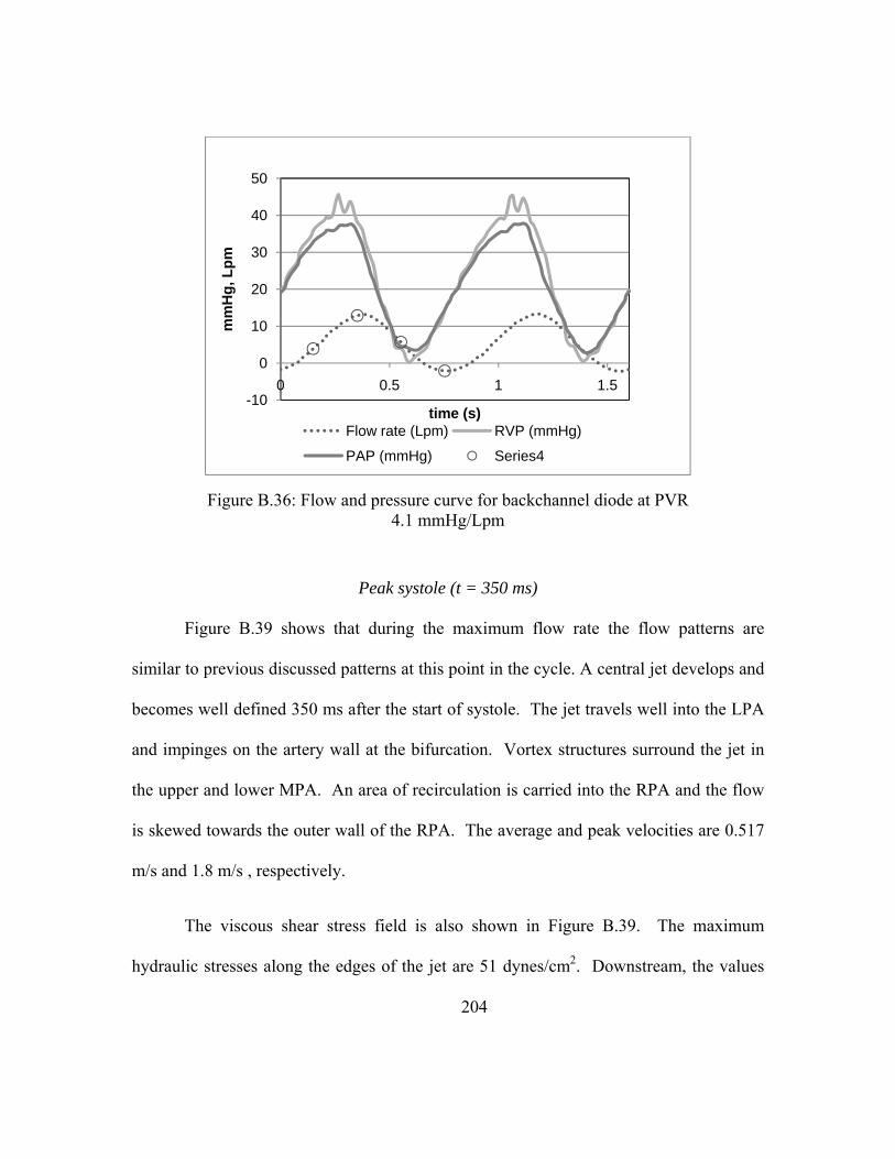
204
Peak systole (t = 350 ms)
Figure B.39 shows that during the maximum flow rate the flow patterns are
similar to previous discussed patterns at this point in the cycle. A central jet develops and
becomes well defined 350 ms after the start of systole. The jet travels well into the LPA
and impinges on the artery wall at the bifurcation. Vortex structures surround the jet in
the upper and lower MPA. An area of recirculation is carried into the RPA and the flow
is skewed towards the outer wall of the RPA. The average and peak velocities are 0.517
m/s and 1.8 m/s , respectively.
The viscous shear stress field is also shown in Figure B.39. The maximum
hydraulic stresses along the edges of the jet are 51 dynes/cm2. Downstream, the values
Figure B.36: Flow and pressure curve for backchannel diode at PVR 4.1 mmHg/Lpm
-10
0
10
20
30
40
50
0 0.5 1 1.5
mm
Hg,
Lpm
time (s)Flow rate (Lpm) RVP (mmHg)
PAP (mmHg) Series4

205
drop to 12 dynes/cm2. There are wall stresses along the lower MPA between 10 – 40
mm. They measure 7 - 16 dynes/cm2. The wall stresses along the distal RPA are as high
as 27 dynes/cm2. Also, at the site of flow impingement, the shear stresses are about 25
dynes/cm2.
The Reynolds shear stresses for peak systole are displayed in Figure B.40. The
regions of elevated Reynolds stresses begin 20 – 22 mm downstream of the valve exit.
The peak stresses are about 800 dynes/cm2 and coincides with the region of recirculation
in the lower main and left pulmonary arteries. The Reynolds shear stresses reach 250
dynes/cm2 at the RPA bend where flow separation begins. Another area of raised
turbulent shear stresses exists, up to 380 dynes/cm2, in the RPA.
Figure B.37: Central plane flow and viscous shear stress (dynes/cm2) field for the backchannel diode at 150 ms after the start of systole for PVR = 4.1
mmHg/Lpm

206
Figure B.39: Central plane flow and viscous shear stress (dynes/cm2) field for the backchannel diode at 350 ms after the start of systole for PVR = 4.1
mmHg/Lpm
Figure B.38: Reynolds shear stress field (dynes/cm2) for the backchannel diode at 150 ms after the start of systole for PVR = 4.1 mmHg/Lpm, central plane

207
Mid diastole (t = 550 ms)
The decelerating flow field for Case 2 is shown in Figure B.41. The central jet
structure is still seen. The peak velocities in the MPA are 0.794 m/s, less than one half of
the peak speeds at 350 ms. The average axial velocity is 0.228 m/s.
The corresponding viscous shear stresses are also mapped in Figure B.41. The
peak stresses along the edges of the jet measure 20 dynes/cm2. The RPA distal wall
stresses were between 9 and 13 dynes/cm2.
Figure B.42 maps the Reynolds shear stresses for the moderate PVR case. The
higher turbulent shear stresses occur in the areas of mixing in the lower LPA and MPA
and just at the branch between the MPA and RPA. In the lower region, the peak stresses
measure 540 dynes/cm2. In the upper region, the peak stresses are 310 dynes/cm2, which
is higher than the observed stresses in the this area at t = 350 ms.

208
Figure B.41: Central plane flow and viscous shear stress (dynes/cm2) field for the backchannel diode at 550 ms after the start of systole for PVR = 4.1
mmHg/Lpm
Figure B.40: Reynolds shear stress (dynes/cm2) field for the backchannel diode at 350 ms after the start of systole for PVR = 4.1 mmHg/Lpm, central plane

209
Diastole (t = 750 ms)
The diastolic flow and viscous shear stress profiles are shown in Figure B.43.
Retrograde flow exists and the profile is uniform in the MPA The secondary flows from
the RPA and LPA are reentering the primary flow. These flows meet at the bifurcation
and this causes the flow in the LPA to be skewed towards the lower wall. . The peak flow
speed in the MPA is -0.186 m/s, and the average flow speed is -0.052 m/s.
The maximum viscous shear stresses are along the walls of the main and left
pulmonary arteries. The values are low, measuring no higher than 4 dynes/cm2.
Figure B.42: Reynolds shear stress (dynes/cm2) field for the backchannel diode at 550 ms after the start of systole for PVR = 4.1 mmHg/Lpm, central
plane

210
In Figure B.44, the Reynolds shear stress field shows low levels of turbulence
within the field. The maximum Reynolds shear stresses are 45 dynes/cm2. This is
located where the retrograde from both branches mix in the MPA.
Backchannel Diode Case 2 - Offset Plane
Early Systole (t = 150 ms)
At 150 ms after the start of the cardiac cycle, the developing jet is visible as seen
in Figure B.45. The span of the jet is expected smaller than in the central plane. As with
the central plane flow, the flow takes on a more uniform profile by 8 mm downstream of
the valve exit. The peak axial velocity is 0.513 m/s. The average is 0.111 m/s. The
viscous shear stresses at t = 150 ms in the offset plane are of similar location and
magnitude as in the central plane (Figure B.45). There is a shear layer that exists at the
edges of the jet exiting the valve orifice. The peak bulk flow shear stresses are around 12
dynes/cm2. The wall stresses are between 3-5 dynes/cm2. The Reynolds shear stresses
are very low (Figure B.46). The maximum RSS measure 13 dynes/cm2.
Peak Systole (t = 350 ms)
The flow mapping for the offset plane during peak systole shows a central jet that
travels the length of MPA shown in Figure B.47. Two areas of recirculation surround the
jet. The peak velocities are 1.67 m/s, less than in the central plane. The average flow
speed is 0.354 m/s. The maximum viscous shear stresses are around 45 dynes/cm2; they
are the same in this plane as they were in the central plane (Figure B.47). Likewise, the
peak stresses are along the edges of the jet. Since the plane of view only covers 22 mm
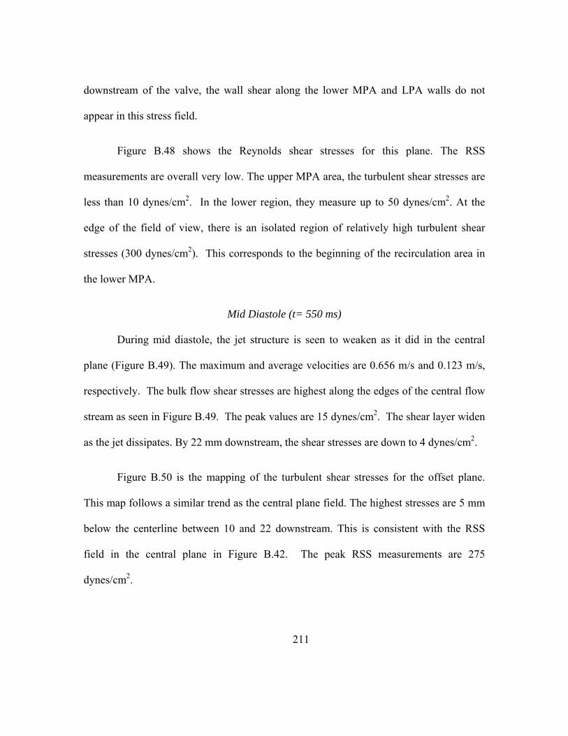
211
downstream of the valve, the wall shear along the lower MPA and LPA walls do not
appear in this stress field.
Figure B.48 shows the Reynolds shear stresses for this plane. The RSS
measurements are overall very low. The upper MPA area, the turbulent shear stresses are
less than 10 dynes/cm2. In the lower region, they measure up to 50 dynes/cm2. At the
edge of the field of view, there is an isolated region of relatively high turbulent shear
stresses (300 dynes/cm2). This corresponds to the beginning of the recirculation area in
the lower MPA.
Mid Diastole (t= 550 ms)
During mid diastole, the jet structure is seen to weaken as it did in the central
plane (Figure B.49). The maximum and average velocities are 0.656 m/s and 0.123 m/s,
respectively. The bulk flow shear stresses are highest along the edges of the central flow
stream as seen in Figure B.49. The peak values are 15 dynes/cm2. The shear layer widen
as the jet dissipates. By 22 mm downstream, the shear stresses are down to 4 dynes/cm2.
Figure B.50 is the mapping of the turbulent shear stresses for the offset plane.
This map follows a similar trend as the central plane field. The highest stresses are 5 mm
below the centerline between 10 and 22 downstream. This is consistent with the RSS
field in the central plane in Figure B.42. The peak RSS measurements are 275
dynes/cm2.

212
Figure B.44: Reynolds shear stress (dynes/cm2) field for the backchannel diode at 750 ms after the start of systole for PVR = 4.1 mmHg/Lpm
Figure B.43: Central plane flow and viscous shear stress (dynes/cm2) field for the backchannel diode at 750 ms after the start of systole for PVR = 4.1
mmHg/Lpm

213
Figure B.46: Offset Reynolds shear stress (dynes/cm2) field at 150 ms after start of systole for backchannel diode at PVR = 4.1 mmHg/Lpm
Figure B.45: Offset plane flow and viscous shear stress (dynes/cm2) field at 150 ms after start of systole for backchannel diode at PVR = 4.1 mmHg/Lpm
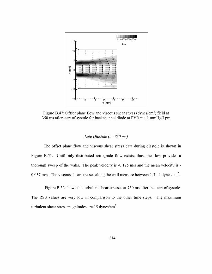
214
Late Diastole (t= 750 ms)
The offset plane flow and viscous shear stress data during diastole is shown in
Figure B.51. Uniformly distributed retrograde flow exists; thus, the flow provides a
thorough sweep of the walls. The peak velocity is -0.125 m/s and the mean velocity is -
0.037 m/s. The viscous shear stresses along the wall measure between 1.5 - 4 dynes/cm2.
Figure B.52 shows the turbulent shear stresses at 750 ms after the start of systole.
The RSS values are very low in comparison to the other time steps. The maximum
turbulent shear stress magnitudes are 15 dynes/cm2.
Figure B.47: Offset plane flow and viscous shear stress (dynes/cm2) field at 350 ms after start of systole for backchannel diode at PVR = 4.1 mmHg/Lpm

215
Figure B.49: Offset plane flow and viscous shear stress (dynes/cm2) field at 550 ms after start of systole for backchannel diode at PVR = 4.1 mmHg/Lpm
Figure B.48: Offset Reynolds shear stress (dynes/cm2) field at 350 ms after start of systole for backchannel diode at PVR = 4.1 mmHg/Lpm

216
Figure B.51: Offset plane flow and viscous shear stress (dynes/cm2) field at 750 ms after start of systole for backchannel diode at PVR = 4.1 mmHg/Lpm
Figure B.50: Offset Reynolds shear stress (dynes/cm2) field at 550 ms after start of systole for backchannel diode at PVR = 4.1 mmHg/Lpm

217
Backchannel Diode - Case 3
The flow and pressure curve for the PVR = 5.1 mmHg/Lpm is shown in Figure
B.53. The regurgitant fraction is 15.0%.
Early Systole (t =150 ms)
At 150 ms after the start of systole, there is uniform, low magnitude antegrade
flow (Figure B.54). There is a complete pass of the artery walls. The average axial
velocity 0.059 m/s and the peak velocity is 0.196 m/s.
Figure B.52: Offset Reynolds shear stress (dynes/cm2) field at 750 ms after start of systole for backchannel diode at PVR = 4.1 mmHg/Lpm

218
The viscous shear stresses are also mapped in Figure B.54. The stresses are
highest along the wall measuring 5 dynes/cm2 in the lower LPA. In the main and right
pulmonary arteries, the stresses are around 2 - 3 dynes/cm2.
Figure B.55 is the mapping of the Reynolds shear stresses 150 ms after the start of
the cardiac cycle. The turbulent stresses are overall very low. There are between -15 and
55 dynes/cm2. The peak RSS is at the exit of the RPA.
Figure B.53: Flow and Pressure Curve for backchannel diode at PVR = 5.1 mmHg/Lpm
150
350
550
750-10
0
10
20
30
40
50
60
0 0.5 1 1.5
mm
Hg,
Lpm
time (s)Flow rate (Lpm) RVP (mmHg)

219
Figure B.55: Reynolds shear stress (dynes/cm2) field for the backchannel diode at 150 ms after the start of systole for PVR = 5.1 mmHg/Lpm
Figure B.54: Central plane flow and viscous shear stress (dynes/cm2) field for the backchannel diode at 150 ms after the start of systole for PVR =5.1
mmHg/Lpm

220
Peak systole (t = 350 ms)
The flow and viscous shear stresses at peak systole are in Figure B.56. A strong
central jet emerges from the valve exit and is best seen in Figure B.56. The jet impinges
on the artery wall at the bifurcation. There is an area of recirculation in the lower MPA
and LPA. Another area is in RPA entrance. The flow along the distal RPA wall is
pronounced as well. The peak velocities within the jet reach 2.07 m/s and the average
velocity in the MPA is 0.611 m/s.
The bulk flow shear stresses are high along the edges of the jet (Figure B.56), at
the lower MPA and LPA walls, and along the distal RPA wall. The maximum shear
stresses are 62 dynes/cm2 at the beginning of the jet stream. The wall stresses in the RPA
are between 34 - 43 dynes/cm2 and up to 17 dynes/cm2 at the lower MPA and LPA walls.
Figure B.57 maps the RSS values for the peak systole case. There is a region in
the lower MPA in the area of recirculation. The peak RSS measurements here are up to
1100 dynes/cm2. Another area of high turbulence is in the upper MPA near the where
flow enters the RPA. The RSS values are as high as 690 dynes/cm2. Finally, in the right
pulmonary artery, there is also a region of elevated stresses ranging up to 490 dynes/cm2.
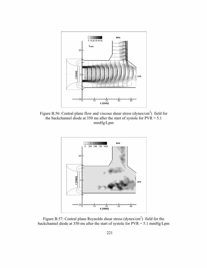
221
Figure B.57: Central plane Reynolds shear stress (dynes/cm2) field for the backchannel diode at 350 ms after the start of systole for PVR = 5.1 mmHg/Lpm
Figure B.56: Central plane flow and viscous shear stress (dynes/cm2) field for the backchannel diode at 350 ms after the start of systole for PVR = 5.1
mmHg/Lpm
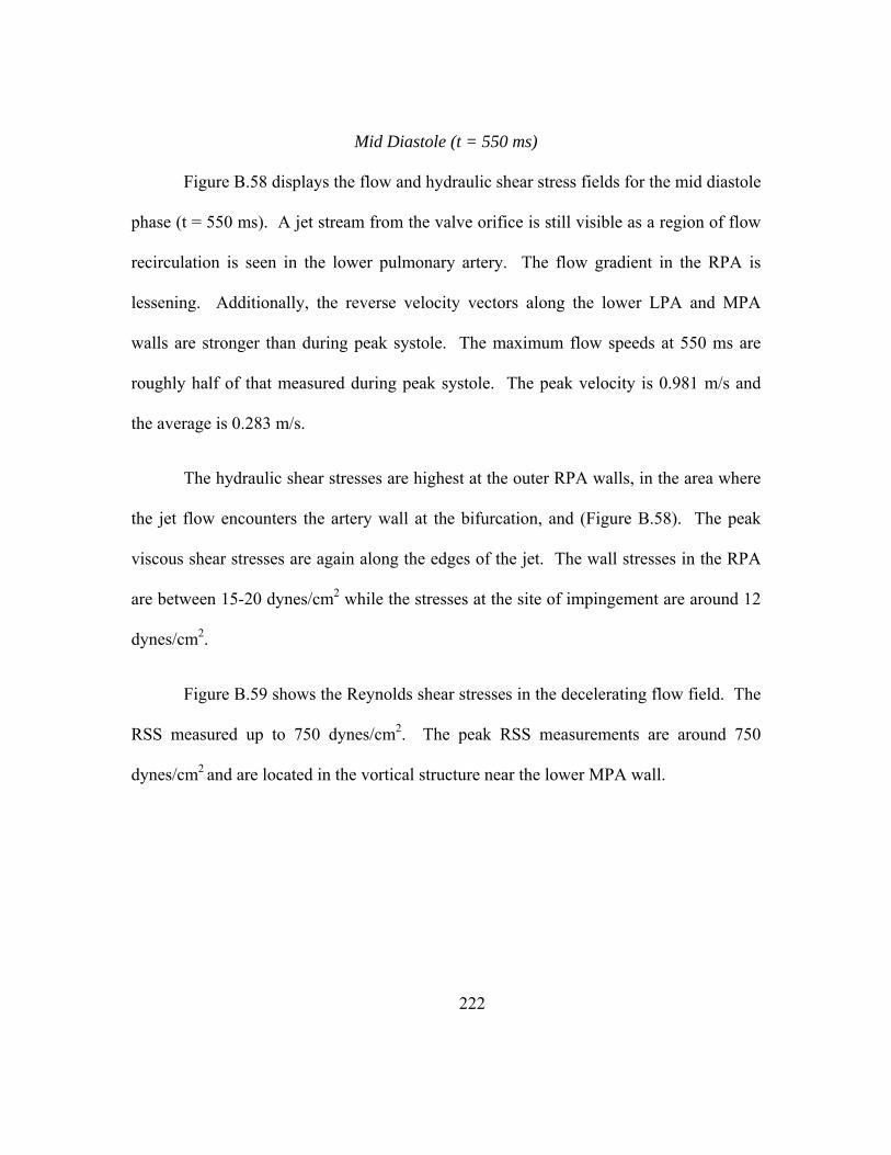
222
Mid Diastole (t = 550 ms)
Figure B.58 displays the flow and hydraulic shear stress fields for the mid diastole
phase (t = 550 ms). A jet stream from the valve orifice is still visible as a region of flow
recirculation is seen in the lower pulmonary artery. The flow gradient in the RPA is
lessening. Additionally, the reverse velocity vectors along the lower LPA and MPA
walls are stronger than during peak systole. The maximum flow speeds at 550 ms are
roughly half of that measured during peak systole. The peak velocity is 0.981 m/s and
the average is 0.283 m/s.
The hydraulic shear stresses are highest at the outer RPA walls, in the area where
the jet flow encounters the artery wall at the bifurcation, and (Figure B.58). The peak
viscous shear stresses are again along the edges of the jet. The wall stresses in the RPA
are between 15-20 dynes/cm2 while the stresses at the site of impingement are around 12
dynes/cm2.
Figure B.59 shows the Reynolds shear stresses in the decelerating flow field. The
RSS measured up to 750 dynes/cm2. The peak RSS measurements are around 750
dynes/cm2 and are located in the vortical structure near the lower MPA wall.

223
Figure B.59: Reynolds shear stress (dynes/cm2) field for the backchannel diode at 550 ms after the start of systole for PVR = 5.1 mmHg/Lpm
Figure B.58: Central plane flow and viscous shear stress (dynes/cm2) field for the backchannel diode at 550 ms after the start of systole for PVR = 5.1 mmHg/Lpm

224
Late Diastole (t = 750 ms)
The flow field during diastole for Case 3 is uniformly distributed retrograde flow
(Figure B.60). In the LPA, the flow is slightly skewed to the lower side. This is a result
of the momentum from the flow from the secondary flows meeting and creating an area
of stasis near the artery branch. The average velocity in the MPA is -0.088 m/s with
velocity reaching maximums at -0.273 m/s.
The uniform flow sweeps the artery walls. This causes elevated wall stresses
along the MPA walls as well as the lower LPA wall and distal RPA wall (Figure B.60).
The peak wall stresses are in the LPA at 8 dynes/cm2. In the main artery, the wall
stresses are just below 5 dynes/cm2 and the wall stresses along the outer RPA are
between 3 – 4 dynes/cm2. There is also a shear layer between the two secondary flow
streams when they converge in the MPA. This shear layer results in bulk flow shear
stresses of around 4 dynes/cm2.
The overall Reynolds shears stresses during diastole are less than 100 dynes/cm2
(Figure B.61). The area of higher turbulent shear stresses coincides with the mixing layer
of the two secondary flows. The RSS are between 50 -75 dynes/cm2 in this location.
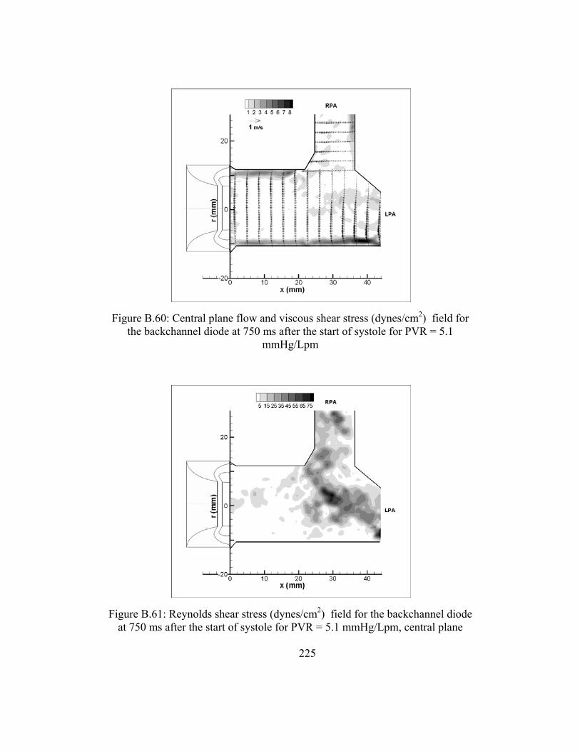
225
Figure B.61: Reynolds shear stress (dynes/cm2) field for the backchannel diode at 750 ms after the start of systole for PVR = 5.1 mmHg/Lpm, central plane
Figure B.60: Central plane flow and viscous shear stress (dynes/cm2) field for the backchannel diode at 750 ms after the start of systole for PVR = 5.1
mmHg/Lpm

226
Backchannel Diode Case 4 - Offset Plane
Early Systole (t = 150 ms)
As the flow begins to accelerate, there is little movement in the flow Figure B.62.
The average speed is -0.036 m/s and the peak is -0.08 m/s. The highest viscous stresses
are at the lower MPA wall with magnitudes up to 4.2 dynes/cm2. In Figure B.63 it is seen
that the stagnant flow leads to little mixing. The turbulent shear stress levels are below 25
dynes/cm2. Peak Systole (t = 350 ms)
The offset flow field at peak systole is shown in Figure B.64. The width of the jet
has narrowed just as the width of the valve orifice is smaller in this plane. There is an
area of recirculation in the lower half of the section. Retrograde flow appears nearest the
valve exit. The axial velocities reach 0.291 m/s on average with peaks of 1.19 m/s.
The bulk flow shear stresses follow the shear layer created by the entrained jet.
The peak shear stresses measure 17.6 dynes/cm2. Also, along the wall where the vortex is
sweeping back the walls, the wall stresses reach 10 dynes/cm2.
The Reynolds shear stresses peak at 283 dynes/cm2 in the offset flow field for this
case (Figure B.65). The highest values are contained in the shear layer created by the
offset jet structure.
Mid Diastole (t = 550 ms)
During the mid diastole, as with Early Systole, there is little activity in the offset
flow field (Figure B.64). The velocities have low magnitudes. The peak speed is 0.280

227
m/s and the average is 0.034 m/s. The jet structure is still visible, albeit small. The flow
along both the upper has reversed so that there is retrograde flow in the outer radial
position. The flow within the first 8 mm of the valve is also flowing back to the valve.
The maximum viscous shear stress is 7.7 dynes/cm2 and is located 18 mm downstream
along the wall.
Figure B.65 shows the Reynolds shear stresses; these values for the offset field of
view reach a maximum at 136 dynes/cm2.
Late Diastole (t =750 ms)
Figure B.68 maps the velocity and hydraulic shear stress fields for the final case
during diastole. Just as it was in the central plane of flow, the velocity profile is uniform.
The average axial flow speed is -0.304 m/s. and the peak speed is -0.580 m/s. The
highest viscous shear stresses measure 14.3 dynes/cm2. The shear stresses along the walls
are higher than those in the flow field.
Figure B.69 maps the RSS field as it occurs during diastole. The highest turbulent
shear stresses are 95 dynes/cm2 and are located 22 mm downstream.
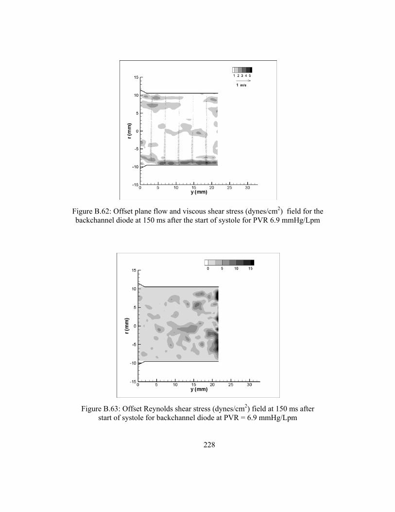
228
Figure B.63: Offset Reynolds shear stress (dynes/cm2) field at 150 ms after start of systole for backchannel diode at PVR = 6.9 mmHg/Lpm
Figure B.62: Offset plane flow and viscous shear stress (dynes/cm2) field for the backchannel diode at 150 ms after the start of systole for PVR 6.9 mmHg/Lpm
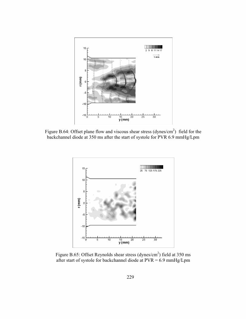
229
Figure B.65: Offset Reynolds shear stress (dynes/cm2) field at 350 ms after start of systole for backchannel diode at PVR = 6.9 mmHg/Lpm
Figure B.64: Offset plane flow and viscous shear stress (dynes/cm2) field for the backchannel diode at 350 ms after the start of systole for PVR 6.9 mmHg/Lpm

230
Figure B.67: Offset Reynolds shear stress (dynes/cm2) field at 550 ms after start of systole for backchannel diode at PVR = 6.9 mmHg/Lpm
Figure B.66: Offset plane flow and viscous shear stress (dynes/cm2) field for the backchannel diode at 550 ms after the start of systole for PVR 6.9 mmHg/Lpm

231
Figure B.69: Offset Reynolds shear stress (dynes/cm2) field at 750 ms after start of systole for backchannel diode at PVR = 6.9 mmHg/Lpm
Figure B.68: Offset plane flow and viscous shear stress (dynes/cm2) field for the backchannel diode at 750 ms after the start of systole for
PVR 6.9 mmHg/Lpm

232
Appendix C
Uncertainty Analysis
This section reports on the uncertainty estimates for results presented in this
dissertation. Elemental errors were identified for each measurement and uncertainties
assigned. Uncertainties were propagated based on the methods detailed in Figliola and
Beasley [123] and ASME PTC 19.1 [124]. In general, for k = 1, 2,... elemental
systematic errors, systematic uncertainties are propagated as
∑ C.1
where θ is the sensitivity factor. In a similar manner, random uncertainties were
propagated as
∑ C.2
with degrees of freedom estimated from the Welch-Sattertwaite formula [124].
Uncertainty in Pressure and Flow Rate Measurements
The contributing source errors to the pressure uncertainty measurements include:
a systematic error based on the manufacturer’s specification, which is assigned standard
systematic uncertainty b; the random error resulting from calibration curve fit, assigned
standard random uncertainty s1 = syx based on the standard error of the curve fit; and the
variation among the multiple data measurements, assigned standard random uncertainty
√ or the standard deviation of the mean of the pressure measurement.

233
The systematic (bRVP) and random uncertainties (sRVP) in the RVP measurement
were found to be ±0.192 mmHg and ±0.199 mmHg, respectively. Likewise, the
uncertainties in the PAP measurement, bPAP and sRVP, were ±0.192 mmHg and ±0.204
mmHg. The systematic uncertainty (bQ) in the flow rate measurement was calculated as
0.050 Lpm. The random uncertainty (sQ) in the flow rate measurement was calculated as
0.126 Lpm. These are shown in Table C. 1.
Uncertainty in TVG and RF% Measurements
Transvalvular Pressure Gradient
Recall that equation 3 states the relationship between the TVG and RVP and PAP
as TVG = RVPpeak - PAPpeak. First, the systemic and random error uncertainties were
found using equations C.3 – C.4.
C.3
C.4
Regurgitant Fraction
The systematic and random uncertainties in the RF% (defined in Equation 2)
resulting from measurement error was found using equations C.5 and C.6.
% % % C.5

234
% % % C.6
Pulmonary Vascular Resistance and Compliance
Equations C.6 and C.7 were used to find the uncertainties in the PVR and PVC
(defined in Equations 6 and 7).
C.7
P C.8
where bmPa = bPAP and smPa = sPAP. The uncertainty in the resulting PVR measurement is
0.19 mmHg/Lpm.
The PVC is a function of the cardiac output, the PA pulse pressure (Pd) and the heart rate.
The bHR was a bias error of ±0.5 bpm. The calculated uncertainties found using equations
C.9 and C.10 for selected points are shown in
∆
PVCHR
C.9
Q C.10

235
Table C. 1. Standard systematic uncertainties (b), random uncertainties (s) and 95% confidence interval uncertainties (u) for all global measurements
Measurement b s u RVP (mmHg) 0.192 0.199 0.541 PAP (mmHg) 0.192 0.204 0.549
Pd (mmHg) 0.192 0.147 0.289 CO (Lpm) 0.050 0.126 0.266
TVG (mmHg) 0.271 0.285 0.771 RF% (32%) 0.006 0.015 0.031 RF%(21%) 0.008 0.020 0.043
PVR (3 mmHg/Lpm) 0.049 0.086 0.194 PVC (2.7 mL/mmHg) 3.80E-05 6.90E-05 1.54E-04
The standard uncertainties of b and s for every measurement are listed in the
Table C. 1. The total 95% confidence interval uncertainties in each measurement are also
reported.
PIV measurements
The main sources for PIV measurement errors are typically particle size, in-plane
loss of particle pairs, seeding density, particle displacement, and background noise [118].
Raffel et al. [118] present results from Monte Carlo simulation work that predict the
effect of these contributors. Based on these results and the conditions of the current study
(64x64 interrogation window, 5-8 pixel displacement), the uncertainty in the pixel
displacement was found using Figures 5.23b, 5.24, 5.27, 5.29, 5.32, and 5.34 published
by Raffel et al. [118]. The values used to determine the uncertainty in pixel displacement
are shown in Table C. 2.
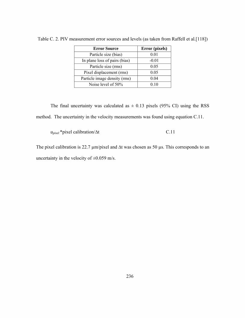
236
Table C. 2. PIV measurement error sources and levels (as taken from Raffell et al.[118])
Error Source Error (pixels) Particle size (bias) 0.01
In plane loss of pairs (bias) -0.01 Particle size (rms) 0.05
Pixel displacement (rms) 0.05 Particle image density (rms) 0.04
Noise level of 50% 0.10
The final uncertainty was calculated as ± 0.13 pixels (95% CI) using the RSS
method. The uncertainty in the velocity measurements was found using equation C.11.
upixel *pixel calibration/∆t C.11
The pixel calibration is 22.7 µm/pixel and ∆t was chosen as 50 µs. This corresponds to an
uncertainty in the velocity of ±0.059 m/s.

237
REFERENCES
1. Shuman, T.M., Heart Disease: Diseases That Affect the Heart and Cardiovascular System, in http://www.webmd.com/content/pages/9/1675_57860.html 2005.
2. Yoganathan, A.P., Z. He, and S. Casey Jones, Fluid mechanics of heart valves. Annu Rev Biomed Eng, 2004. 6: p. 331-62.
3. Butany, J., M.S. Ahluwalia, C. Munroe, C. Fayet, C. Ahn, P. Blit, C. Kepron, R.J. Cusimano, and R.L. Leask, Mechanical heart valve prostheses: identification and evaluation. Cardiovasc Pathol, 2003. 12(1): p. 1-22.
4. Waterbolk, T.W., E.S. Hoendermis, I.J. den Hamer, and T. Ebels, Pulmonary valve replacement with a mechanical prosthesis. Promising results of 28 procedures in patients with congenital heart disease. Eur J Cardiothorac Surg, 2006. 30(1): p. 28-32.
5. Butany, J., C. Fayet, M.S. Ahluwalia, P. Blit, C. Ahn, C. Munroe, N. Israel, R.J. Cusimano, and R.L. Leask, Biological replacement heart valves. Identification and evaluation. Cardiovasc Pathol, 2003. 12(3): p. 119-39.
6. Bonhoeffer, P., Y. Boudjemline, Z. Saliba, J. Merckx, Y. Aggoun, D. Bonnet, P. Acar, J. Le Bidois, D. Sidi, and J. Kachaner, Percutaneous replacement of pulmonary valve in a right-ventricle to pulmonary-artery prosthetic conduit with valve dysfunction. The Lancet, 2000. 356(9239): p. 1403-1405.
7. Berne, R. and M. Levy, Cardiovascular Physiology. 1992, Boston: Mosby Year Book.
8. Levick, J., An Introduction to Cardiovascular Physiology. 1995, Oxford: Butterworth-Heinmann Ltd.
9. Weinberg, C.E., J.R. Hertzberg, D.D. Ivy, K.S. Kirby, K.C. Chan, L. Valdes-Cruz, and R. Shandas, Extraction of pulmonary vascular compliance, pulmonary vascular resistance, and right ventricular work from single-pressure and Doppler flow measurements in children with pulmonary hypertension: a new method for evaluating reactivity: in vitro and clinical studies. Circulation, 2004. 110(17): p. 2609-17.
10. Mousseaux, E., J.P. Tasu, O. Jolivet, G. Simonneau, J. Bittoun, and J.C. Gaux, Pulmonary arterial resistance: noninvasive measurement with indexes of pulmonary flow estimated at velocity-encoded MR imaging--preliminary experience. Radiology, 1999. 212(3): p. 896-902.
11. Slife, D.M., R.D. Latham, P. Sipkema, and N. Westerhof, Pulmonary arterial compliance at rest and exercise in normal humans. Am J Physiol, 1990. 258(6 Pt 2): p. H1823-8.
12. Rosendorff, C., Essential Cardiology: Principles and Practice. 2001, New York: W.B. Saunders.

238
13. American Heart Association, I., Congenital Cardiovascular Defects: Statistics. 2009.
14. Pulmonary Valve Disease. 2009, Mayo Clinic. 15. Alexander, R., Hurst's The Heart. 9th ed. 1998, New York: McGraw-Hill. 16. Adults With Congenital Heart Disease: The Normal Heart and How It Works.
2006: http://www.americanheart.org/presenter.jhtml?identifier=11064. 17. Tariq, M., R.A. Smego, Jr., A. Soofi, and N. Islam, Pulmonic valve endocarditis.
South Med J, 2003. 96(6): p. 621-3. 18. de Ruijter, F.T., I. Weenink, F.J. Hitchcock, E.J. Meijboom, and G.B. Bennink,
Right ventricular dysfunction and pulmonary valve replacement after correction of tetralogy of Fallot. Ann Thorac Surg, 2002. 73(6): p. 1794-800; discussion 1800.
19. Therrien, J., S.C. Siu, P.R. McLaughlin, P.P. Liu, W.G. Williams, and G.D. Webb, Pulmonary valve replacement in adults late after repair of tetralogy of fallot: are we operating too late? J Am Coll Cardiol, 2000. 36(5): p. 1670-5.
20. Warner, K.G., P.K. O'Brien, J. Rhodes, A. Kaur, D.A. Robinson, and D.D. Payne, Expanding the indications for pulmonary valve replacement after repair of tetralogy of fallot. Ann Thorac Surg, 2003. 76(4): p. 1066-71; discussion 1071-2.
21. Yemets, I.M., W.G. Williams, G.D. Webb, D.A. Harrison, P.R. McLaughlin, G.A. Trusler, J.G. Coles, I.M. Rebeyka, and R.M. Freedom, Pulmonary valve replacement late after repair of tetralogy of Fallot. Ann Thorac Surg, 1997. 64(2): p. 526-30.
22. Tulevski, II, A. Hirsch, A. Dodge-Khatami, J. Stoker, E.E. van der Wall, and B.J. Mulder, Effect of pulmonary valve regurgitation on right ventricular function in patients with chronic right ventricular pressure overload. Am J Cardiol, 2003. 92(1): p. 113-6.
23. Conte, S., R. Jashari, B. Eyskens, M. Gewillig, M. Dumoulin, and W. Daenen, Homograft valve insertion for pulmonary regurgitation late after valveless repair of right ventricular outflow tract obstruction. Eur J Cardiothorac Surg, 1999. 15(2): p. 143-9.
24. Bloomfield, P., Choice of heart valve prosthesis. Heart, 2002. 87(6): p. 583-9. 25. Gott, V.L., D.E. Alejo, and D.E. Cameron, Mechanical heart valves: 50 years of
evolution. Ann Thorac Surg, 2003. 76(6): p. S2230-9. 26. Yoganathan, A.P., K.B. Chandran, and F. Sotiropoulos, Flow in prosthetic heart
valves: state-of-the-art and future directions. Ann Biomed Eng, 2005. 33(12): p. 1689-94.
27. Bluestein, D., Y.M. Li, and I.B. Krukenkamp, Free emboli formation in the wake of bi-leaflet mechanical heart valves and the effects of implantation techniques. J Biomech, 2002. 35(12): p. 1533-40.
239
28. Ilbawi, M.N., C.G. Lockhart, F.S. Idriss, S.Y. DeLeon, A.J. Muster, C.E. Duffy, and M.H. Paul, Experience with St. Jude Medical valve prosthesis in children. A word of caution regarding right-sided placement. J Thorac Cardiovasc Surg, 1987. 93(1): p. 73-9.
29. Miyamura, H., H. Kanazawa, J. Hayashi, and S. Eguchi, Thrombosed St. Jude Medical valve prosthesis in the right side of the heart in patients with tetralogy of Fallot. J Thorac Cardiovasc Surg, 1987. 94(1): p. 148-50.
30. Reiss, N., U. Blanz, H. Bairaktaris, A. Koertke, and R. Korfer, Mechanical valve replacement in congenital heart defects in the era of international normalized ratio self-management. Asaio J, 2005. 51(5): p. 530-2.
31. Rosti, L., B. Murzi, A.M. Colli, P. Festa, S. Redaelli, and A. Frigiola, Pulmonary valve replacement: a role for mechanical prostheses? Ann Thorac Surg, 1998. 65(3): p. 889-90.
32. Burger, W., G.D. Kneissl, A. Hartmann, R. Bauersachs, V. Doring, U. Spengler, G. Neumann, and K.W. Rothe, Successful thrombolysis after prosthetic pulmonary valve obstruction under aspirin monotherapy. Ann Thorac Surg, 1997. 64(1): p. 255-7; discussion 257-8.
33. Iscan, H.Z., M. Seren, D.S. Kucukaksu, and K. Bayazit, Mechanical heart valve prosthesis in the pulmonary position without anticoagulation: case report. J Heart Valve Dis, 2004. 13(1): p. 149-51.
34. Kiyota, Y., T. Shiroyama, T. Akamatsu, Y. Yokota, and T. Ban, In vitro closing behavior of the St. Jude Medical heart valve in the pulmonary position. Valve incompetence originating in the prosthesis itself. J Thorac Cardiovasc Surg, 1992. 104(3): p. 779-85.
35. Meuris, B., E. Verbeken, and W. Flameng, Mechanical valve thrombosis in a chronic animal model: differences between monoleaflet and bileaflet valves. J Heart Valve Dis, 2005. 14(1): p. 96-104.
36. Chang, B.C., S.H. Lim, D.K. Kim, J.Y. Seo, S.Y. Cho, W.H. Shim, N. Chung, S.S. Kim, and B.K. Cho, Long-term results with St. Jude Medical and CarboMedics prosthetic heart valves. J Heart Valve Dis, 2001. 10(2): p. 185-194; discussion195.
37. Buttard, P., E. Bonnefoy, P. Chevalier, P.B. Marcaz, J. Robin, J.F. Obadia, G. Kirkorian, and P. Touboul, Mechanical cardiac valve thrombosis in patients in critical hemodynamic compromise. Eur J Cardiothorac Surg, 1997. 11(4): p. 710-3.
38. Deviri, E., P. Sareli, T. Wisenbaugh, and S.L. Cronje, Obstruction of mechanical heart valve prostheses: clinical aspects and surgical management. J Am Coll Cardiol, 1991. 17(3): p. 646-50.
39. Emery, R.W., C.A. Erickson, K.V. Arom, W.F. Northrup, 3rd, T.E. Kersten, T.J. Von Rueden, T.J. Lillehei, and D.M. Nicoloff, Replacement of the aortic valve in patients under 50 years of age: long-term follow-up of the St. Jude Medical prosthesis. Ann Thorac Surg, 2003. 75(6): p. 1815-9.
240
40. Gohean, J., R. Figliola, T. Camp, and T. McQuinn, Comparative in vitro study of bileaflet and tilting disk valve behavior in the pulmonary position. ASME J Biomechanical Engineering, 2006. 128(4): p. 631-5.
41. Malouf, J.F., H.M. Hannoush, and J.A. Odell, Fractured occluder disc: a previously unrecognized complication of the Starr-Edwards disc prosthesis. J Heart Valve Dis, 2001. 10(1): p. 136-8.
42. Haas, F., C. Schreiber, J. Horer, M. Kostolny, K. Holper, and R. Lange, Is there a role for mechanical valved conduits in the pulmonary position? Ann Thorac Surg, 2005. 79(5): p. 1662-7; discussion 1667-8.
43. Fukada, J., K. Morishita, K. Komatsu, and T. Abe, Influence of pulmonic position on durability of bioprosthetic heart valves. Ann Thorac Surg, 1997. 64(6): p. 1678-80; discussion 1680-1.
44. Lurz, P. and P. Bonhoeffer, Percutaneous implantation of pulmonary valves for treatment of right ventricular outflow tract dysfunction. Cardiology in the Young, 2008. 18(03): p. 260-267.
45. Lurz, P., R. Gaudin, A.M. Taylor, and P. Bonhoeffer, Percutaneous Pulmonary Valve Implantation. Seminars in Thoracic and Cardiovascular Surgery: Pediatric Cardiac Surgery Annual, 2009. 12(1): p. 112-117.
46. Woo, Y.R. and A.P. Yoganathan, In vitro pulsatile flow velocity and shear stress measurements in the vicinity of mechanical mitral heart valve prostheses. J Biomech, 1986. 19(1): p. 39-51.
47. Hellums, J.D., 1993 Whitaker Lecture: biorheology in thrombosis research. Ann Biomed Eng, 1994. 22(5): p. 445-55.
48. Hung, T.C., R.M. Hochmuth, J.H. Joist, and S.P. Sutera, Shear-induced aggregation and lysis of platelets. Trans Am Soc Artif Intern Organs, 1976. 22: p. 285-91.
49. Kroll, M.H., J.D. Hellums, L.V. McIntire, A.I. Schafer, and J.L. Moake, Platelets and shear stress. Blood, 1996. 88(5): p. 1525-41.
50. Leverett, L.B., J.D. Hellums, C.P. Alfrey, and E.C. Lynch, Red blood cell damage by shear stress. Biophys J, 1972. 12(3): p. 257-73.
51. Sallam, A.M. and N.H. Hwang, Human red blood cell hemolysis in a turbulent shear flow: contribution of Reynolds shear stresses. Biorheology, 1984. 21(6): p. 783-97.
52. Stein, P.D. and H.N. Sabbah, Measured turbulence and its effect on thrombus formation. Circ Res, 1974. 35(4): p. 608-14.
53. Stein, P.D. and H.N. Sabbah, Hemorheology of turbulence. Biorheology, 1980. 17(4): p. 301-19.
54. Ramstack, J.M., L. Zuckerman, and L.F. Mockros, Shear-Induced Activation of Platelets. Biomechanics, 1979. 12: p. 113-125.
55. Bluestein, D., L. Niu, R. Schoephoerter, and M.K. Dewanjee, Fluid Mechanics of Arterial Stenosis: Relationship to the Development of Mural Thrombus. Annals of Biomedical Engineering, 1997. 25: p. 344-356.

241
56. Yoganathan, A.P., Y.R. Woo, and H.W. Sung, Turbulent shear stress measurements in the vicinity of aortic heart valve prostheses. J Biomech, 1986. 19(6): p. 433-42.
57. Figliola, R.S. and T.J. Mueller, On the hemolytic and thrombogenic potential of occluder prosthetic heart valves from in-vitro measurements. J Biomech Eng, 1981. 103(2): p. 83-90.
58. Stein, P.D., F.J. Walburn, and H.N. Sabbah, Turbulent stresses in the region of aortic and pulmonary valves. J Biomech Eng, 1982. 104(3): p. 238-44.
59. Lim, W.L., Y.T. Chew, T.C. Chew, and H.T. Low, Pulsatile flow studies of a porcine bioprosthetic aortic valve in vitro: PIV measurements and shear-induced blood damage. J Biomech, 2001. 34(11): p. 1417-27.
60. Giersiepen, M., L. Wurzinger, R. Opitz, and H. Reul, Estimation of shear stress-related blood damage in heart valve prostheses--in vitro comparison of 25 aortic valves. The International Journal of Artificial Organs, 1990. 13(5): p. 300-6.
61. Bluestein, D., E. Rambod, and M. Gharib, Vortex shedding as a mechanism for free emboli formation in mechanical heart valves. J Biomech Eng, 2000. 122(2): p. 125-34.
62. Holme, P.A., U. Orvim, M.J.A.G. Hamers, N.O. Solum, F.R. Brosstad, R.M. Barstad, and K.S. Sakariassen, Shear-Induced Platelet Activation and Platelet Microparticle Formation at Blood Flow Conditions as in Arteries With a Severe Stenosis. Arterioscler Thromb Vasc Biol, 1997. 17(4): p. 646-653.
63. Davis, M.E., H. Cai, G.R. Drummond, and D.G. Harrison, Shear Stress Regulates Endothelial Nitric Oxide Synthase Expression Through c-Src by Divergent Signaling Pathways. Circ Res, 2001. 89(11): p. 1073-1080.
64. Niebauer, M., Josef and M. Cooke, PhD, FACC, John P., Cardiovascular Effects of Exercise; Role of Endothelial Shear Stress. Journal of the American College of Cardiology, 1996. 28(7): p. 1652-1660
65. Zeshuai, X., Z. Zhaohui, and L.D. Scott, Shear stress induction of the endothelial nitric oxide synthase gene is calcium-dependent but not calcium-activated. Journal of Cellular Physiology, 1997. 171(2): p. 205-211.
66. Khalighi, B., K.B. Chandran, and C.J. Chen, Steady flow development past valve prostheses in a model human aorta. II. Tilting disc valves. J Biomech, 1983. 16(12): p. 1013-8.
67. Khalighi, B., K.B. Chandran, and C.J. Chen, Steady flow development past valve prostheses in a model human aorta. I. Centrally occluding valves. J Biomech, 1983. 16(12): p. 1003-11.
68. Lim, W.L., Y.T. Chew, T.C. Chew, and H.T. Low, Steady flow dynamics of prosthetic aortic heart valves: a comparative evaluation with PIV techniques. J Biomech, 1998. 31(5): p. 411-21.
69. Bluestein, D. and S. Einav, The effect of varying degrees of stenosis on the characteristics of turbulent pulsatile flow through heart valves. J Biomech, 1995. 28(8): p. 915-24.

242
70. Chandran, K.B., T.L. Yearwood, C.J. Chen, and H.L. Falsetti, PULSATILE FLOW EXPERIMENTS ON HEART VALVE PROTHESES. Medical & Biological Engineering & Computing, 1983. 21(5): p. 529-537.
71. Chandran, K.B., Pulsatile flow past St. Jude Medical bileaflet valve. An in vitro study. J Thorac Cardiovasc Surg, 1985. 89(5): p. 743-9.
72. Chandran, K.B., R. Schoephoerster, R. Fatemi, and E.L. Dove, An in vitro experimental comparison of Edwards-Duromedics and St Jude bileaflet heart valve prostheses. Clin Phys Physiol Meas, 1988. 9(3): p. 233-41.
73. Subramanian, A., H. Mu, J.R. Kadambi, M.P. Wernet, A.M. Brendzel, and H. Harasaki, Particle image velocimetry investigation of intravalvular flow fields of a bileaflet mechanical heart valve in a pulsatile flow. J Heart Valve Dis, 2000. 9(5): p. 721-31.
74. Manning, K.B., V. Kini, A.A. Fontaine, S. Deutsch, and J.M. Tarbell, Regurgitant flow field characteristics of the St. Jude bileaflet mechanical heart valve under physiologic pulsatile flow using particle image velocimetry. Artif Organs, 2003. 27(9): p. 840-6.
75. Pantalos, G.M., S.C. Koenig, K.J. Gillars, and D.L. Ewert. Mock circulatory system for testing cardiovascular devices. 2002. Houston, TX, United States: Institute of Electrical and Electronics Engineers Inc.
76. Liu, Y., P. Allaire, H. Wood, and D. Olsen, Design and initial testing of a mock human circulatory loop for left ventricular assist device performance testing. Artif Organs, 2005. 29(4): p. 341-5.
77. Pantalos, G.M., S.C. Koenig, K.J. Gillars, G.A. Giridharan, and D.L. Ewert, Characterization of an Adult Mock Circulation for Testing Cardiac Support Devices. ASAIO Journal, 2004. 50(1): p. 37-46.
78. Timms, D., M. Hayne, K. McNeil, and A. Galbraith, A complete mock circulation loop for the evaluation of left, right, and biventricular assist devices. Artif Organs, 2005. 29(7): p. 564-72.
79. Philpot, E., In vitro Flow Visualization and Pressure Measurement Studies in Pulmonary Artery. 1984, Georgia Institute of Technology: Atlanta.
80. Philpot, E., A.P. Yoganathan, H.W. Sung, Y.R. Woo, R.H. Franch, D.J. Sahn, and L. Valdez-Cruz, In-vitro pulsatile flow visualization studies in a pulmonary artery model. J Biomech Eng, 1985. 107(4): p. 368-75.
81. Sung, H.W., T.L. Hsu, C.H. Hsu, and J.C. Hsu, Pulmonary artery hemodynamics with varying degrees of valvular stenosis: an in vitro study. J Biomech, 1998. 31(12): p. 1153-61.
82. Yin, W., I.B. Krukenkamp, A.E. Saltman, G. Gaudette, K. Suresh, O. Bernal, J. Jesty, and D. Bluestein, Thrombogenic performance of a st. Jude bileaflet mechanical heart valve in a sheep model. Asaio J, 2006. 52(1): p. 28-33.
83. Irwin, E., G. Lang, R. Clack, J. St Cyr, W. Runge, J. Foker, and R. Bianco, Long-term evaluation of prosthetic mitral valves in sheep. J Invest Surg, 1993. 6(2): p. 133-41.

243
84. Semb, B.K., A. Aasen, G. Woxholt, F. Resch, A.M. Refsum, T. Froysaker, S. Nitter-Hauge, K. Stadsklev, and P. Lilleaasen, In vivo haemodynamic evaluation of the Hall-Kaster central flow prosthetic heart valve. Scand J Clin Lab Invest, 1979. 39(8): p. 731-6.
85. Choo, S.J., K.I. Kim, N.H. Park, J.M. Song, I.C. Choi, J.Y. Shim, S.K. Lee, Y.J. Kwon, C.N. Kim, and J.W. Lee, Development of an animal experimental model for a bileaflet mechanical heart valve prosthesis. J Korean Med Sci, 2004. 19(1): p. 37-41.
86. Salerno, C.T., J. Droel, and R.W. Bianco, Current state of in vivo preclinical heart valve evaluation. J Heart Valve Dis, 1998. 7(2): p. 158-62.
87. Knudsen, L.L., H.R. Andersen, and J.M. Hasenkam, Catheter-implanted prosthetic heart valves. Transluminal catheter implantation of a new expandable artificial heart valve in the descending thoracic aorta in isolated vessels and closed chest pigs. Int J Artif Organs, 1993. 16(5): p. 253-62.
88. Gross, D.R., M.K. Dewanjee, P. Zhai, S. Lanzo, and S.M. Wu, Successful prosthetic mitral valve implantation in pigs. Asaio J, 1997. 43(5): p. M382-6.
89. Bluestein, D., W. Yin, K. Affeld, and J. Jesty, Flow-induced platelet activation in mechanical heart valves. J Heart Valve Dis, 2004. 13(3): p. 501-8.
90. Akutsu, T. and T. Fukuda, Time-resolved particle image velocimetry and laser doppler anemometry study of the turbulent flow field of bileaflet mechanical mitral prostheses. J Artif Organs, 2005. 8(3): p. 171-83.
91. Akutsu, T., R. Imai, and Y. Deguchi, Effect of the flow field of mechanical bileaflet mitral prostheses on valve closing. J Artif Organs, 2005. 8(3): p. 161-70.
92. Browne, P., A. Ramuzat, R. Saxena, and A.P. Yoganathan, Experimental investigation of the steady flow downstream of the St. Jude bileaflet heart valve: a comparison between laser Doppler velocimetry and particle image velocimetry techniques. Ann Biomed Eng, 2000. 28(1): p. 39-47.
93. Brucker, C., U. Steinseifer, W. Schroder, and H. Reul, Unsteady flow through a new mechanical heart valve prosthesis analysed by digital particle image velocimetry. Measurement Science & Technology, 2002. 13(7): p. 1043-1049.
94. Castellini, P., M. Pinotti, and L. Scalise, Particle image velocimetry for flow analysis in longitudinal planes across a mechanical artificial heart valve. Artif Organs, 2004. 28(5): p. 507-13.
95. Kini, V., C. Bachmann, A. Fontaine, S. Deutsch, and J.M. Tarbell, Integrating particle image velocimetry and laser Doppler velocimetry measurements of the regurgitant flow field past mechanical heart valves. Artif Organs, 2001. 25(2): p. 136-45.
96. Lim, W.L., Y.T. Chew, T.C. Chew, and H.T. Low, Particle image velocimetry in the investigation of flow past artificial heart valves. Ann Biomed Eng, 1994. 22(3): p. 307-18.

244
97. Pierrakos, O., P.P. Vlachos, and D.P. Telionis, Time-resolved DPIV analysis of vortex dynamics in a left ventricular model through bileaflet mechanical and porcine heart valve prostheses. J Biomech Eng, 2004. 126(6): p. 714-26.
98. Baldwin, J.T., S. Deutsch, H.L. Petrie, and J.M. Tarbell, Determination of principal reynolds stresses in pulsatile flows after elliptical filtering of discrete velocity measurements. J Biomech Eng, 1993. 115(4A): p. 396-403.
99. Maymir, J.C., S. Deutsch, R.S. Meyer, D.B. Geselowitz, and J.M. Tarbell, Mean velocity and Reynolds stress measurements in the regurgitant jets of tilting disk heart valves in an artificial heart environment. Ann Biomed Eng, 1998. 26(1): p. 146-56.
100. Meyer, R.S., S. Deutsch, J.C. Maymir, D.B. Geselowitz, and J.M. Tarbell, Three-component laser Doppler velocimetry measurements in the regurgitant flow region of a Bjork-Shiley monostrut mitral valve. Ann Biomed Eng, 1997. 25(6): p. 1081-91.
101. Liu, J.S., P.C. Lu, and S.H. Chu, Turbulence characteristics downstream of bileaflet aortic valve prostheses. J Biomech Eng, 2000. 122(2): p. 118-24.
102. Chandran, K.B., G.N. Cabell, B. Khalighi, and C.J. Chen, Laser anemometry measurements of pulsatile flow past aortic valve prostheses. J Biomech, 1983. 16(10): p. 865-73.
103. Figliola, R.S., In vitro velocity and stress measurements in the vicinity of prosthetic heart valves. 1979, Notre Dame.
104. Tesla, N., Valvular Conduit. 1920: United States. 105. Thoma, D., Fluid Lines. 1932: United States. 106. Berlin, J.H. and F. Paris, Aerodynamic Valve. 1954. 107. Paul, F., Fluid Mechanics of the Momentum Flueric Diode. 1968, Lehigh
Univeristy. 108. Kilner, P.J., R. Balossino, G. Dubini, S.V. Babu-Narayan, A.M. Taylor, G.
Pennati, and F. Migliavacca, Pulmonary regurgitation: the effects of varying pulmonary artery compliance, and of increased resistance proximal or distal to the compliance. Int J Cardiol, 2009. 133(2): p. 157-66.
109. Losaw, J., in vitro Analysis of Prosthetic Heart Valves in the Pulmonary Position, in Mechanical Engineering. 2004, Clemson University: Clemson.
110. Bean, H., Fluid Meters: Their Theory and Application. 6 ed. 1971 New York: ASME. 111. Figliola, R.S., A Study of the Hemolytic Potential of Prosthetic Heart Valve Flows
Based on Local In Vitro Stress Measurements. 1976, Notre Dame. 112. Gohean, J., R. Figliola, T. Camp, and T. McQuinn, Comparative In Vitro Study of
Bileaflet and Tilting Disk Valve Behavior in the Pulmonary Position. Journal of Biomechanical Engineering, 2006. 128(4): p. 631-635.
113. Brimioulle, S., M. Maggiorini, J. Stephanazzi, F. Vermeulen, P. Lejeune, and R. Naeije, Effects of low flow on pulmonary vascular flow-pressure curves and pulmonary vascular impedance. Cardiovasc Res, 1999. 42(1): p. 183-92.

245
114. Haft, J.W., P. Montoya, O. Alnajjar, S.R. Posner, J.L. Bull, M.D. Iannettoni, R.H. Bartlett, and R.B. Hirschl, An artificial lung reduces pulmonary impedance and improves right ventricular efficiency in pulmonary hypertension. J Thorac Cardiovasc Surg, 2001. 122(6): p. 1094-100.
115. Huez, S., S. Brimioulle, R. Naeije, and J.L. Vachiery, Feasibility of routine pulmonary arterial impedance measurements in pulmonary hypertension. Chest, 2004. 125(6): p. 2121-8.
116. Milnor, W., Hemodynamics. 1989, New York: Williams & Wilkins. 117. Cardiovascular Implants: Cardiac Valve Prostheses. 2005, ANSI/AAMI/ISO
5840: Arlington, VA. 118. Raffel, M., C. Willert, and J. Kompenhans, Particle Image Velocimetry, ed. R.J.
Adrian, Gharib, M., Merzhirch, W., Rockwell, D, Whitelaw, J. H. 1998, Berlin: Springer.
119. Camp, T.A., K.C. Stewart, R.S. Figliola, and T. McQuinn, In Vitro Study of Flow Regulation for Pulmonary Insufficiency. ASME J Biomechanical Engineering, 2007. 129(2).
120. Yoganathan, A.P. and B.R. Travis, Fluid Dynamics of Prosthetic Valves, in Practice of Clinical Endocardiography. 2000: Philadelphia.
121. Mount, L.E. and D.L. Ingram, The Pig as a Laboratory Animal. 1971, New York, NY: Academic Press.
122. Conover, T., Multi-Scale Model of a Fluid Diode. 2008, Clemson University. p. 1-5.
123. Figliola, R. and D. Beasley, Theory and Design for Mechanical Measurements. 4th ed. 2005, New York: Wiley.
124. ASME, PTC 19.1 - 2005 Test Uncertainty. 2005.