Evaluation of design and optimization software for Additive Manufacturing with focus on topology optimization

Degree Project in

Industrial Engineering and Management, Second Cycle, 30 Credits

Stockholm, Sweden June 2016

Diego Della Crociata

Supervisor

Amir Rashid

Examiner

Lasse Wingård

Abstract During the past years, new production processes have been developed which build adding step by

step layers on the previous ones. These techniques are referred to as 3D printing or Additive

Manufacturing (AM).

The introduction of metals among the materials available to manufacture parts led to revolutionary

developments in the manufacturing field.

The first consequence of using such techniques is the freedom of design that can be assigned by the

designer, thus implying the production of complex parts. Another benefit is the reduction of waste

material. Aerospace and automotive industries are trying to exploit AM, to obtain high performance

with weight and cost savings.

Full potential of design freedom can be realised by making effective use of topology optimization

(TO). It helps to reduce the weight of the structures while keeping the same performance, or even

enhancing it.

However, the potential of TO can be only exploited if combined with AM, since the results given by

the topology optimization simulations are sometimes complex shapes, which can be produced only

by the AM process regardless of the layout of the part being fabricated.

In this project the optimization of an automotive upright is performed, in order to take advantage to

reduce its weight. An investigation of topology optimization results carried out on Alumec 89 (the

original material for the upright), titanium alloy Ti6Al4V and steel AISI 4142 is performed. The aim

is to reduce weight and improve the performance by changing to titanium, but other aspects need to

be taken into account. If the reduction of weight is not followed by effectiveness from the technical

and economical point of views, the design option cannot be selected.

The aim is to also investigate if an optimization on the aluminium component gives feasible results,

or changing to steel can be an economical option even with an increase in the weight.

In the first part of the present work topology optimization approach is presented. Then the advantages

of combining TO and AM are highlighted. Following this the challenge in design of the upright is

presented along with description of materials investigated for its design. In addition, the cost and

environmental impact considerations are also discussed.

In the second part, which is the experimental one, at first the software explored for performing the

optimization are presented: Siemens NX 8.5, Inspire 2015, ParetoWorks 2016 within Solidworks,

ANSYS 14.0, Within 2016. Afterwards the design analysis settings, along with the results coming from

each software (benefits and limitations as well) are described. The best software will be chosen,

according to the preset objectives. SolidThinking Inspire 2015 turned out to be the best TO software,

since it is able to cover most of the steps through the concept of the design to the actual production i

of the component. In addition, the material that suits the most to this work is aluminium alloy. It can

withstand the stress acting on the component (even after material reduction), it is a material with no

high price and it can be easily recycled.

ii

Sammanfattning Under de förgångna åren har nya produktionsprocesser framkallats som bygger att tillfoga steg-för-

steg lager på de föregående. Dessa tekniker kallas Friformsframställning (FFF).

Inledningen av metaller bland de tillgängliga materialen som tillverkar delar som ledas till

revolutionära utvecklingar i det fabriks- fältet.

Den första följden av att använda sådana tekniker är friheten av designen, som kan tilldelas av

disegneren som således antyder produktionen av komplexa delar. En annan fördel är förminskningen

av förlorat material. Rymd och bilindustrier försöker att exploatera FFF, att erhålla hög kapacitet med

vikt och att kosta besparingar.

Full spänning av designfrihet kan realiseras, genom att göra effektivt bruk av topologioptimering

(TO). Den hjälper att förminska vikten av strukturerna, medan hålla den samma kapaciteten eller

förhöja även den.

Hursomhelst, spänningen av TO kan endast exploateras, om kombinerat med FFF, sedan resultaten

som ges av topologioptimeringsimuleringarna, är ibland komplexa former, som kan produceras

endast av FFF-processen utan hänsyn till orienteringen av delen som fabriceras.

I detta projekt utförs optimizationen av en automatisk styrspindel, för att ta fördel för att förminska

dess vikt. En utredning av topologioptimeringresultat bar ut på Alumec 89 (det original- materialet

av spindeln), titanlegeringen Ti6Al4V, och stål AISI 4142 utförs. Syftet är att förminska vikt och

förbättra kapaciteten, genom att ändra till titan, men andra aspekter behöver tas in i konto. Om

förminskningen av vikt inte följs av effektivitet från den tekniska och ekonomiska punkten av sikter,

kan designalternativet inte vara utvalt.

Syftet är också att utforska, om en optimization på den aluminium delen ger görliga resultat, eller att

ändra till stål kan vara ett ekonomiskt alternativ även med en förhöjning i vikten.

I den första delen av närvarande arbetstopologioptimering framläggas inställningen. Därefter

markeras fördelarna av att kombinera TO och FFF. Efter detta framläggas utmaningen i designen av

uprighten tillsammans med beskrivning av material som utforskas för dess design. I tillägg diskuteras

kostnads- och miljöpåverkanövervägandena också.

I den andra delen som är den experimentella, först framläggas programvaran som undersöks för att

utföra optimering: Siemens NX 8,5, Inspire 2015, ParetoWorks 2016 inom Solidworks, ANSYS 14,0,

Within2016. Därefter beskrivas designanalysinställningarna, tillsammans med resultaten som

kommer från varje programvara (fördelar och begränsningar som väl).

Den bästa programvaran ska väljas, enligt förinställningsmålen. SolidThinking Inspire 2015 som ut

vänds för att vara det bästa TO programvara, sedan det är i stånd till att täcka mest av momenten till

och med begreppet av designen till den faktiska produktionen av delen. I tillägg är materialet, som iii

passar mest till detta arbete, den aluminium legeringen. Det kan motstå spänningen som agerar på

delen (även efter materiell förminskning), det är ett material med inget högt pris, och det kan lätt

återanvändas.

iv

Acknowledgments First of all, I would like to thank my supervisor professor Amir Rashid for giving me the possibility

to do a research in a field of interest for me and which I studied in detail during my Erasmus

experience. His enthusiasm towards the area was important for the choice of my master thesis’ topic,

and having a relationship on a par with him was a great aspect of Swedish educational system.

I thank Johan Petterson for helping me with the computer issues at university and obtaining most of

the licenses I needed for working on my degree project. I really appreciate him being always available

to solve the students’ problems.

I thank Per Johansson for helping me in getting a license and for his precious suggestions.

I would also like to express my appreciation to the Formula Student at KTH for allowing me to

contributing with my work in an attempt to bring the optimization revolution into students’ level.

A thank goes also to Praveen Yadav from Paretoworks and Angela Giordano from solidThinking for

helping me further after providing me a license for the software.

I would like to express my gratitude towards professor Luca Iuliano, who accepted to be my

supervisor at Politecnico di Torino. His continuous support and suggestions were of great importance

for the connection with my home university.

I thank all the students I met during this experience. Meeting guys from different countries and

cultures was really important for me growing as a person other than as a student. In particular Umer,

Anup, Maria, Meixin, Tirou at university and the guys from Tyresö accommodation, especially

Alessio, Giulia and Luca.

I cannot forget my friends in Italy, who have always supported me: Alberto, Alberto, Alessandra,

Elizabeth, Francesco, Jordy, Leonardo, Marco, Marco, Matteo, Santo, Stefano and Vito.

However, the first thank goes to the members of my family, because if I managed to realize what I

accomplished it is thank to them. I would have never done anything without their support, and I will

never forget it.

v

List of acronyms In this work, some acronyms will be used to refer to some terms. Here is a list of them:

• AM = Additive Manufacturing

• TO = Topology Optimization

• UCA = Upper Control Arm

• LCA = Lower Control Arm.

vi

Table of contents 1. INTRODUCTION .................................................................................................................................. 1

2. SOFTWARE DESCRIPTION ............................................................................................................... 3

3. TOPOLOGY OPTIMIZATION ........................................................................................................... 5

3.1 Introduction to Optimization .................................................................................................................. 5

3.2 Classification of the optimization methods: size, shape, topology optimization .................................... 5

3.3 Topology optimization ........................................................................................................................... 6

3.3.1 A brief note on the history ............................................................................................................... 6

3.3.2 Classification of topology optimization methods ............................................................................. 7

3.3.3 Problems related to post processing within topology optimization ................................................ 21

3.3.4 Correlation between topology optimization and additive manufacturing ....................................... 23

4. APPLICATION OF TOPOLOGY OPTIMIZATION....................................................................... 25

4.1 Case study ............................................................................................................................................ 25

4.1.1 Geometry of the upright................................................................................................................. 27

4.1.2 Stress analysis ................................................................................................................................ 28

4.2 Challenge: switching from aluminium to titanium. Possible risks. Investigation of optimization with aluminium and steel as well........................................................................................................................ 32

4.3 Research questions ............................................................................................................................... 34

5. MATERIAL DESCRIPTION .............................................................................................................. 35

5.1 Titanium: description of properties and application in additive manufacturing .................................... 35

5.2 Alumec 89 ............................................................................................................................................ 36

5.3 Steel AISI 4142 .................................................................................................................................... 37

6. BUSINESS CONSIDERATION .......................................................................................................... 38

7. ENVIRONMENTAL IMPACT FROM USING ADDITIVE MANUFACTURING ....................... 41

8. NUMERICAL SECTION .................................................................................................................... 44

8.1 ANSYS Mechanical 14.0 ..................................................................................................................... 44

8.2 SolidThinking Inspire 2015 .................................................................................................................. 49

8.2.1 Ti6Al4V ........................................................................................................................................ 50

8.2.2 Alumec 89 ..................................................................................................................................... 56

8.2.3 Steel AISI 4142 ............................................................................................................................. 59

8.3 Siemens NX 8.5 .................................................................................................................................... 63

8.4 ParetoWorks 2016 ................................................................................................................................ 72

8.4.1 Ti6Al4V ........................................................................................................................................ 72

8.4.2 Alumec 89 ..................................................................................................................................... 79

8.4.3 Steel AISI 4142 ............................................................................................................................. 83

8.5 Autodesk Within 2016 .......................................................................................................................... 87

vii

8.5.1 Ti6Al4V ........................................................................................................................................ 88

8.5.2 Alumec 89 ..................................................................................................................................... 93

8.5.3 Steel AISI 4142 ............................................................................................................................. 94

9. CONCLUSIONS ................................................................................................................................... 96

APPENDIX ................................................................................................................................................. 100

Post-processing for braking and cornering analysis with Paretoworks ..................................................... 100

ANSYS Mechanical 14.0 – more results .................................................................................................. 105

Siemens NX 8.5 – more results ................................................................................................................ 106

REFERENCES ........................................................................................................................................... 108

LIST OF FIGURES REFERENCES ........................................................................................................ 110

viii

List of figures Figure 2.1 - Comparison between software ...................................................................................................... 4 Figure 3.1 Michell truss layout for loaded plate ............................................................................................... 5 Figure 3.2 SMS method result .......................................................................................................................... 8 Figure 3.3 Solution to EA ............................................................................................................................... 11 Figure 3.4 Morphological representation of geometry within EA .................................................................. 12 Figure 3.5 Flow chart of BESO ...................................................................................................................... 14 Figure 3.6 Input problem ................................................................................................................................ 15 Figure 3.7 Output problem ............................................................................................................................. 16 Figure 3.8 Flow chart of SIMP ....................................................................................................................... 20 Figure 3.9 Mesh dependency example for SIMP ............................................................................................ 21 Figure 3.10 Situation to avoid ........................................................................................................................ 22 Figure 4.1 2016 Competition Upright, overview 1 ......................................................................................... 25 Figure 4.2 2016 Competition Upright, overview 2 ......................................................................................... 26 Figure 4.3 Geometry and connections of the upright ...................................................................................... 27 Figure 4.4 Reference system for the loads calculation.................................................................................... 29 Figure 4.5 Surfaces with acting moments ....................................................................................................... 31 Figure 6.1 Comparison between costs due to AM and conventional techniques ............................................ 38 Figure 7.1 Environmental impact of conventional and innovative techniques ................................................ 42 Figure 8.1 Workbench screen after the definition steps .................................................................................. 45 Figure 8.2 Constraints with UCA connection, Ansys 14.0 Figure 8.3 Constraints with steering mechanism, Ansys 14.0 ...................................................................................................................................................... 46 Figure 8.4 Constraints with LCA connection, Ansys 14.0 ................................................................................ 46 Figure 8.5 Definition of the forces, Ansys 14.0 .............................................................................................. 47 Figure 8.6 Retaining the shown surface, Ansys 14.0 Figure 8.7 Retaining the shown surface, Ansys 14.0 ................................................................................................................................................................ 47 Figure 8.8 Retaining the shown surface, Ansys 14.0 ...................................................................................... 48 Figure 8.9 Simulation result with Mechanical ................................................................................................ 48 Figure 8.10 Upright subdivision in Inspire 2015 ............................................................................................ 50 Figure 8.11 Constraint with UCA connection, Inspire 2015 ........................................................................... 51 Figure 8.12 Constraints with steering mechanism, Inspire 2015 .................................................................... 51 Figure 8.13 Constraints with LCA connection, Inspire 2015 .......................................................................... 52 Figure 8.14 Loads application, Inspire 2015 .................................................................................................. 52 Figure 8.15 Optimization result Ti6Al4V - overview ..................................................................................... 53 Figure 8.16 Optimization result Ti6Al4V - lower detail Figure 8.17 Optimization result Ti6Al4V - upper detail ............................................................................................................................................................... 53 Figure 8.18 Displacement results Ti6Al4V .................................................................................................... 54 Figure 8.19 Percent of yield results Ti6Al4V ................................................................................................. 54 Figure 8.20 Von Mises results Ti6Al4V ......................................................................................................... 55 Figure 8.21 Von Mises results Ti6Al4V - detail ............................................................................................. 55 Figure 8.22 Optimization results Alumec 89 - overview ................................................................................ 56 Figure 8.23 Optimization results Alumec 89 - upper detail Figure 8.24 Optimization results Alumec 89 - lower detail ..................................................................................................................................................... 56 Figure 8.25 Displacement results Alumec 89 ................................................................................................. 57 Figure 8.26 Percent of yield results Alumec 89 .............................................................................................. 57 Figure 8.27 Percent of yield results Alumec 89 - detail 1 Figure 8.28 Percent of yield results Alumec 89 - detail 2 ............................................................................................................................................................ 58 Figure 8.29 Von Mises results Alumec 89...................................................................................................... 58

ix

Figure 8.30 Von Mises results Alumec 89 - detail.......................................................................................... 58 Figure 8.31 Optimization results steel AISI 4142 - overview ......................................................................... 59 Figure 8.32 (on the left) Optimization results steel AISI 4142 - upper detail ................................................. 60 Figure 8.33 (on the right) Optimization results steel AISI 4142 - lower detail ............................................... 60 Figure 8.34 Displacement results steel AISI 4142 .......................................................................................... 60 Figure 8.35 Percent of yield results steel AISI 4142 ...................................................................................... 61 Figure 8.36 Percent of yield results steel AISI 4142 - detail .......................................................................... 61 Figure 8.37 Von Mised stress results steel AISI 4142 .................................................................................... 62 Figure 8.38 Von Mised stress results steel AISI 4142 - detail ........................................................................ 62 Figure 8.39 Connection of the .fem file to the .prt file, NX 8.5 ...................................................................... 64 Figure 8.40 Settings for creating the mesh, NX 8.5 ........................................................................................ 64 Figure 8.41 Connection of .sim file to .fem file, NX 8.5 ................................................................................ 65 Figure 8.42 Simulation settings, NX 8.5 ........................................................................................................ 65 Figure 8.43 Constraint with UCA connection, NX 8.5 ................................................................................... 66 Figure 8.44 Constraint with steering mechanism, NX 8.5 .............................................................................. 66 Figure 8.45 Constraint with LCA connection, NX 8.5 ................................................................................... 67 Figure 8.46 Overview of the loads applied, NX 8.5 ....................................................................................... 67 Figure 8.47 Design space - detail 1, NX 8.5 ................................................................................................... 68 Figure 8.48 Design space - detail 2, NX 8.5 ................................................................................................... 68 Figure 8.49 Non-design space, NX 8.5 ........................................................................................................... 69 Figure 8.50 Design responses in NX 8.5 ........................................................................................................ 69 Figure 8.51 Constraint defined in NX 8.5....................................................................................................... 70 Figure 8.52 Optimization result - overview .................................................................................................... 70 Figure 8.53 Optimization result - detail 1 Figure 8.54 Optimization results - detail 2 .................. 71 Figure 8.55 Initialization in Paretoworks 2016 for Ti6Al4V .......................................................................... 73 Figure 8.56 Constraint with UCA connection, Paretoworks 2016 .................................................................. 73 Figure 8.57 Costraint with steering mechanism connection, Paretoworks 2016 ............................................. 74 Figure 8.58 Constraint with LCA connection, Paretoworks 2016 .................................................................. 74 Figure 8.59 Overview of loads applied, Paretoworks 2016 ............................................................................ 75 Figure 8.60 Surfaces retain overview, Paretoworks 2016 ............................................................................... 75 Figure 8.61 FEA settings for Ti6Al4V, Paretoworks 2016 ............................................................................. 76 Figure 8.62 Topology optimization simulation settings for Ti6Al4V, Paretoworks 2016 .............................. 76 Figure 8.63 Optimization results – overview Figure 8.64 Optimization results - detail 1 ........ 77 Figure 8.65 Optimization results - detail 2 Figure 8.66 Optimization results - detail 3 ................. 77 Figure 8.67 Von Mises stress results Ti6Al4V ............................................................................................... 78 Figure 8.68 Displacement results Ti6Al4V .................................................................................................... 78 Figure 8.69 Initialization in Paretoworks 2016 for Alumec 89 ....................................................................... 79 Figure 8.70 Loads, constraints and surface retain for Alumec 89, Paretoworks 2016 .................................... 79 Figure 8.71 FEA settings for Alumec 89, Paretoworks 2016 ......................................................................... 80 Figure 8.72 Topology optimization simulation settings for Alumec 89, Paretoworks 2016 ........................... 80 Figure 8.73 Optimization results - overview .................................................................................................. 81 Figure 8.74 Optimization results - detail 1 Figure 8.75 Optimization results - detail 2 ...... 81 Figure 8.76 Von Mises stress results for Alumec 89 ...................................................................................... 82 Figure 8.77 Displacement results for Alumec 89 ........................................................................................... 82 Figure 8.78 Initialization in Paretoworks 2016 for steel AISI 4142 ............................................................... 83 Figure 8.79 Loads, constraints and surface retains overview for steel AISI 4142, Paretoworks 2016 ............ 83 Figure 8.80 FEA settings for steel AISI 4142, Paretoworks 2016 .................................................................. 84 Figure 8.81 Topology optimization simulation settings for steel AISI 4142, Paretoworks 2016 .................... 84

x

Figure 8.82 Optimization results – overview Figure 8.83 Optimization results - detail .............. 85 Figure 8.84 Von Mises stress results steel AISI 4142..................................................................................... 86 Figure 8.85 Displacement results steel AISI 4142 .......................................................................................... 86 Figure 8.86 Lattice structure overview, Within 2016 ..................................................................................... 88 Figure 8.87 Constraint with UCA connection, Within 2016 ........................................................................... 89 Figure 8.88 Constraint with steering mechanism connection, Within 2016 .................................................... 89 Figure 8.89 Constraint with LCA connection, Within 2016 ........................................................................... 90 Figure 8.90 Loads application on the upright, Within 2016 ........................................................................... 90 Figure 8.91 Von Mises stress result Ti6Al4V................................................................................................. 91 Figure 8.92 Simulation results Ti6Al4V, Within 2016 ................................................................................... 91 Figure 8.93 Optimization settings Ti6Al4V, Within 2016 .............................................................................. 92 Figure 8.94 No optimization required screen, Within 2016 ............................................................................ 92 Figure 8.95 Von Mises stress results Alumec 89 ............................................................................................ 93 Figure 8.96 Simulation results Alumec 89, Within 2016 ................................................................................ 94 Figure 8.97 No optimization required for Alumec 89, Within 2016 ............................................................... 94 Figure 8.98 Von Mises stress results steel AISI 4142..................................................................................... 95 Figure 8.99 Simulation results steel AISI 4142, Within 2016 ........................................................................ 95 Figure 9.1 - Comparison between the final shapes (Inspire, Paretoworks and Within, from left to right) ...... 97 Figure A.1 - Manually optimized component, detail 1 Figure A.0.2 - Manually optimized component, detail 2 .......................................................................................................................................................... 100 Figure A.3 - displacement result, titanium alloy ........................................................................................... 101 Figure A.4 - percent of yield result, titanium alloy ....................................................................................... 101 Figure A.5 - displacement result, aluminium alloy ....................................................................................... 102 Figure A.6 - percent of yield result, aluminium alloy ................................................................................... 102 Figure A.7 - displacement result, steel alloy ................................................................................................. 103 Figure A.8 - percent of yield result, steel alloy ............................................................................................. 103 Figure A.9 - Von Mises stress results ........................................................................................................... 104 Figure A.10 - Overview with fine mesh ....................................................................................................... 105 Figure A.11 - Fine mesh, detail 1 Figure A.12 - Fine mesh, detail 2 ................ 105 Figure A.13 - Overview with 2 mm mesh, simulation 1 ............................................................................... 106 Figure A.14 - 2 mm mesh, detail 1, simulation 1 Figure A.15 - 2 mm mesh, detail 2, simulation 1 .................................................................................................................................................. 106 Figure A.16 - Overview with 2 mm mesh, simulation 2 ............................................................................... 107 Figure A.17 - 2 mm mesh, detail 1, simulation 2 Figure A.18 - 2 mm mesh, detail 2, simulation 2 ................................................................................................................................................................... 107

xi

1. INTRODUCTION

During the past years, manufacturing industry has seen revolutionary changes in the way the products

are fabricated. New production processes are actually being developed which build adding step by

step layers on the previous ones while binding them. These techniques are referred to as Additive

Manufacturing (AM), while at the beginning they were called 3D printing and then Rapid Prototyping

since it was possible to produce only prototypes. They include several processes based on the way

the 3D printed part is generated or on the material used for manufacturing it.

A focus should be posed on the fact that, while at the beginning only processes allowing to produce

prototypes were available (Rapid Prototyping), progress in the field brought to the development of

techniques which permit to create tools (Rapid Tooling) or end parts. One of the factors for such a

revolution was the introduction of metals among the materials available to manufacture parts, apart

from the polymers which were the first introduced in the market.

This has given the possibility to the industries to start producing actual parts by using such processes,

thus bringing some benefits to their products. The first consequence is the freedom of design that can

be assigned by the designer, thus implying the production of complex parts for improving

performance in the actual use. Another benefit is the reduction of waste material, since material is

added during the process, instead of removing it through subtractive techniques. Of course the first

trying to take advantage of this technology were aerospace and automotive industries, where high

performance are required.

One of the best examples that can be presented is the one from the Airbus A380 [1]. In that case a

weight saving of over 1000 kg was achieved.

The next step in the way to improve the manufacturing process is using an optimization method.

There are actually three possibilities, sometimes even combined together in order to exploit the

benefits of each of them. They are size, shape and topology optimization.

The choice for this study is topology optimization (TO), which is a mathematical approach for

optimizing material layout within a provided design space. The aim is to reach performance targets,

and in order to accomplish so a proper set of loads and constraints need to be provided. The main

purpose is actually to reduce the weight of the structures while keeping the same performance, if

possible even enhancing them. TO offers an enormous possibility to the manufacturers, since

decreasing the weight of the structures allows to reach important results such as lightening of critical

parts thus improving their performance, decreasing of emissions thanks to lighter structures, cost

savings since less material is needed for the process (so less waste of material). 1

However, the potential of TO can be only exploited if combined with AM, since the results given by

the topology optimization simulations are sometimes complex shapes, which can be produced only

by an AM process regardless of the layout of the part being fabricated.

In this project the optimization of an upright, a component of the Racing Car from Formula Student

at KTH, is performed.

The work has been carried out by exploring five different software providing the possibility of

optimizing components: Siemens NX 8.5, solidThinking Inspire 2015, ParetoWorks 2016 within

Solidworks, Ansys 14.0 and its pre-installed optimization plug-in, Autodesk Within 2016.

Each software has been investigated in order to understand the possibilities offered along with the

limitations. In fact, some of them are relatively new released software, because optimization is a

relatively new research field. Therefore, in some software not all the features are allowed, and they

will be presented afterwards.

Moreover, they use different methods for performing optimizations, thus giving different shape

results. These methods are different in that they use different objective parameters or algorithms.

After the evaluation of the several software, simulations using three different materials are performed

in the most suitable software:

• Alumec 89

• Ti6Al4V

• Steel AISI 4142.

2

2. SOFTWARE DESCRIPTION In this chapter a first overview of the software involved in the project is presented.

In this way, it is possible to understand how each of them works.

They are in fact different one from each other, covering a different number of steps during the process

between the concept of the component design to the manufacture of the same.

ANSYS Mechanical 14.0 allows to meshing the model, running a Finite Element Analysis (FEA) on

it and optimizing the same component with the integrated shape optimization module. If one wants

to create the geometry of an item (in this case it was imported with a neutral format) there are other

packages within Workbench.

SolidThinking Inspire 2015 permits to create a model, run an FEA with a defined background mesh,

optimize the component and analyse the optimized result from the topology simulation. It can work

by importing and exporting different file format, that is why it is flexible in the designers’ work.

Siemens NX 8.5 is a CAD software including the additional topology optimization plug-in. Hence,

after the possibility to create a model and run an FEA, a topology optimization is available along with

an automatic analysis of the optimized component.

Paretoworks 2016 is an add-on provided by SciArt, LLC. It works within Solidworks environment,

and does not give the possibility to create a component itself. However, after opening it, it is possible

to run an FEA on the component (after defining the number of elements in which the component

would be split) and a topology optimization simulation. The software automatically analyses the

optimized model.

Autodesk Within 2016 is a topology optimization software on its own. It does not permit to create

components, that is why they can only be imported within the software. However, it is possible to

create a component with lattice structure inside, which is then analysed and, if the loads acting on it

are higher than a threshold imposed by design, the optimized component can also be further

optimized. The trends of stress and displacement are automatically determined.

3

Figure 2.1 - Comparison between software

4

3. TOPOLOGY OPTIMIZATION

3.1 Introduction to Optimization The possibility offered by Additive Manufacturing in producing components with complex shapes

provided motivation to investigate methods to design structures with the aim of minimizing the

weight disregarding design complexity which is an issue in case of traditional manufacturing

techniques.

The first work heading to this direction dates back to the early 1900s by A. G. M. Michell [2].

Mathematical conditions under which weight of structure can be decreased were developed. The

revolution coming from this research is that it is possible to minimize structures weight if they contain

trusses, which are members with only tension-compression acting on them.

In figure 3.1 a Michell truss layout is shown for a common loaded plate structural problem.

Figure 3.1 Michell truss layout for loaded plate

However, Michell truss layout gives optimal results only for simple 2D cases. For more complex ones

numerical procedures for obtaining approximate solutions were developed.

3.2 Classification of the optimization methods: size, shape, topology optimization According to [2], “optimization methods seek to improve the design of an artifact by adjusting values

of design variables in order to achieve desired objectives, typically related to structural performance

or weight, as well as possible without violating constraints”.

Three kinds of problems can be distinguished, which are:

5

- Size optimization

- Shape optimization

- Topology optimization

They are presented in an order of increasing scope and complexity.

They all have some objectives to be satisfied: for example, minimization of maximum stress, strain

energy, deflection, volume or weight. They can also be used as constraints.

Size optimization is about determining the values of defined dimensions in order to achieve objectives

in the best way whilst satisfying constraints. Usually the number of size dimensions is small, but it

can increase with complex structures, such as cellular structures.

Shape optimization can be described as the generalization of the previous method. It deals with

optimizing the shape of bounding curves and surfaces while trying to satisfy objectives and

constraints, too. Design variables can be the position of control vertices for curves or surfaces.

It is possible to use shape and size optimization together to optimize structures with free-form shapes

or standard shapes with dimensions.

Even for topology optimization there are objectives and constraints to satisfy, however it is about

determining the overall shape, arranging shape elements and connecting the design domain.

There are big differences, which are in the starting geometric configuration and the choice of

variables, between the latter and the former methods. Topology optimization is the considered method

for this research since it can lead to important improvements in structural performance.

3.3 Topology optimization 3.3.1 A brief note on the history Topology optimization is a method which determines the overall configuration of shape elements of

the component being designed. It is such a powerful tool that its results can be afterwards used for

size or shape optimization problems. This method exploits finite element analysis during every

6

iteration of the process, thus possibly causing really demanding simulations. Usually the solutions

produced by this method are nearly fully stressed or have constant strain energy throughout the

geometry.

As previously stated, the birth of topology optimization dates back to the beginning of the 20th

century [3]. The first work was done by an Australian inventor, Michell in 1904. In fact he developed

optimality criteria for minimizing the weight for trusses structures.

Michell’s theory was investigated again and extended by G. I. N. Rozvany and his research group to

grillages. The work was afterwards used by Rozvany and Prager to formulate the first general theory

of topology optimization. This can be applied to different structures, such as continuum-type

structures, even though they applied it mainly to grid-type structures.

The theory revolutionized the research in this field in such a way that many papers dealt with

extensions of it, for example the work by Lewinski and Rozvany in trying to get exact solutions of

popular benchmark problems.

However, it is thank to the important work by Bendsoe and Kikuchi in 1988 that an intensive

investigation on numerical methods for topology optimization took place.

3.3.2 Classification of topology optimization methods

According to [4], “Topology optimization is a computational material distribution method for

synthesizing structures without any preconceived shape”.

A classification for the topology optimization approaches developed is the following:

- Truss-based methods

- Volume-based density methods.

7

I) Truss-based methods

Truss-based approach deals with defining a volume of interest where a mesh of struts connecting a

set of nodes is set.

The optimization simulations allow to determine the important struts which have to be kept, the size

and remove the ones with small sizes. This approach is strictly dependent on the starting mesh of

struts, thus affecting quality.

In the beginning, the truss-based methods were about having a ground truss defined over a grid of

nodes, and every node was linked to the others by a truss element.

The design variable was each element’s diameter. This helped in determining the elements with

decreasing diameter, so that the small ones could be removed.

However, this approach, which gave good results, was computationally expensive.

In order to overcome such a problem, researchers found new methods that use a different problem

formulation such as including background meshes and analytical derivatives for computing the

sensitivities.

In order to obtain good results, it is required to use truss element size along with position as design

variables.

There are also more methods that use heuristic optimization methods. The aim is to reduce the number

of design variables in the problem.

One of the methods is Size Matching and Scaling (SMS). It has a conformal lattice structure and

requires two design variables, minimum and maximum strut diameters.

Figure 3.2 SMS method result

It is possible to get optimized results by performing a finite element analysis on a solid body. 8

Within the latter a conformal lattice structure fitting the solid body is realized. It is possible to use

local strain or stress values resulting from the analysis to scale struts in the lattice structure.

It is possible then to perform size optimization over the lattice structure in order to evaluate the

maximum and minimum diameters.

II) Volume-based density methods

This approach deals with the determination of the proper material density in a set of voxels that

include a spatial domain.

A description of the main methods follows.

a) Homogenization

A way to make the compliance problem well-posed is to use the homogenization method. It basically

deals with relaxing the binary condition (material or void) thus including intermediate material

density while formulating the problem [4]. This allows the chattering configurations to become part

of the problem statement by assuming a periodically perforated microstructure. Following the name

of the method, the homogenization theory is used to determine the mechanical properties of the

material.

However, some issues emerge from this method. Among them, the main is that the optimal

microstructure for the derivation of the relaxed problem is not always known.

This forces to use some solutions, such as the partial relaxation, which is about restricting the method

to a subclass of microstructures, which should be suboptimal but fully explicit.

This optimization method implies another issue, which is the actual manufacturability of the obtained

component.

In fact, the grey areas found in the optimized structure contain microscopic length-scale holes, which

are almost impossible to fabricate. A way to overcome it is to use penalization strategies. For example,

an a posteriori one deals with post processing the result obtained from the partial relaxation and

forcing the intermediate densities to be black or white. This is however a purely numerical and mesh

dependent strategy.

A priori strategy is instead about imposing restrictions on the microstructures that lead to black and

white designs.

A drawback deriving from the use of optimization methods is that the problem goes back to the ill-

posedness with respect to mesh refinement. 9

b) Soft kill option

SKO inspires from nature. Actually, energy cost is required to produce and maintain materials that

compose a structure. Hence, it is better for a biology to reduce the amount of material in its structure.

In nature, structures tend to reduce material by assuming shapes that distribute stresses as uniformly

as possible [5].

This method resembles in some ways SIMP (Solid Isotropic Material with Penalization) method and

BESO (Bidirectional Evolutionary Structural Optimization) technique, while in others it is different

[6].

In fact, it is similar to SIMP method as it uses a finite element grid and allows the use of fractional

material properties in it.

Conversely, it uses fractional elastic properties instead of fractional densities for defining the quantity

of material needed in the grid elements.

In addition, it resembles BESO technique as, in each iteration, it adds or removes elements according

to the stress state on them.

Each element is assigned a value for Young modulus (E) in the interval [Emin, Emax] according to its

temperature. In turn, it can be a value within [0, 100] and is determined as a function of the element’s

stress state. The temperature is only a means for scaling material properties.

The characteristic emerging for this method is that stresses are the optimization objectives.

Actually, the purpose is to find a geometry where there is a uniform distribution of the stresses, σref.

In order to obtain such a result, each node in the grid is assigned a temperature Tk(i), determined in

each iteration as:

𝑇𝑇𝑘𝑘(𝑖𝑖) = 𝑇𝑇𝑘𝑘(𝑖𝑖−1) + 𝑠𝑠�𝜎𝜎𝑘𝑘 − 𝜎𝜎𝑟𝑟𝑟𝑟𝑟𝑟�, (1)

where 𝑇𝑇𝑘𝑘(𝑖𝑖−1) is the value in the previous iteration, 𝜎𝜎𝑘𝑘 is the principal Von Mises stress in the point

and s is a factor.

In this way, the reference stress is reached with a speed proportional to the difference between current

and reference stress.

Hence, the result is a structure with a uniform stress distribution.

It is possible to consider technological constraints within this method.

10

c) Evolutionary based algorithms

This method discretizes the domain in a rectangular grid of square finite elements for 2D problems,

while hexahedral elements for 3D problems [6].

Every element in the grid is assigned a binary value, which can assume either 0 when the element

represents a hole or 1 if the element represents material.

The main issue related to this method is that it is population based, so the number of individuals

forming the population has to be of the same magnitude order as the number of optimization

parameters, otherwise the algorithm does not converge. That is why these algorithms are

computationally expensive; for example, for 3D domains tens or hundreds of thousands of fitness

function evaluations are required.

A way to decrease the number of fitness evaluations is to generate the optimal solution over a series

of steps, each with an increasing refinement in the grid and increasing chromosome. Moreover, each

step uses the best result of the previous one as starting point, until a sufficiently refined solution is

obtained. An example is shown in figure 3.3.

Figure 3.3 Solution to EA

The use of EA within topology optimization can lead to structure connectivity problems since the

domain is represented in a discrete way and the algorithms have a stochastic character. That is the

reason why some solutions have been suggested, for example starting from seed elements and then

considering as material only the elements connected to them. However, for 3D cases the problem is

more complex, so the discontinuity increases.

Recently a new approach was proposed for this method, that is using a morphological representation

of the geometry. In order to do so, the primitives representing the geometry are spline curves or

NURBS surfaces.

The geometry can be created in a CAD software and the optimization be performed on the CAD

specification tree.

In figure 3.4 an example of topology optimization analysis performed by using such an approach is

presented.

11

Figure 3.4 Morphological representation of geometry within EA

The advantage of using morphological approach is that it provides a CAD model with the optimized

result, instead of giving results in a form that needs interpretation.

d) Evolutionary Structural Optimization methods

The ESO methods use a discrete design space, so they resemble SIMP, but they are hard kill methods,

since each element in the domain assumes a value of density of either 1 or 0, that is either material or

hole [6].

At the beginning, ESO method was proposed, where the design space was filled with material and

then it was removed where not needed in the iterations.

The name is not completely appropriate, because evolutionary refers to Darwinian processes (it is the

same for genetic algorithms) and optimization should be used to indicate the computation of an

optimal solution; however, this has been proven not to be the case for ESO [3]. A proper term would

be SERA, which stands for Sequential Element Rejections and Admissions.

Afterwards a variation was developed, that is AESO, or additive evolutionary structural optimization.

In this case, the structure is composed at first by connections of the seed points (that is, loads and

supports) that are the minimum number of elements to accomplish this. Then elements are added in

each iteration around the elements with high sensitivity.

Thereafter, in order to take the best from both the methods, BESO was introduced, which stands for

bidirectional evolutionary structural optimization.

During the several iterations, it removes inefficient elements but also adds new ones where required.

There have been attempts to make this method independent of grid resolution.

The BESO problem is formulated as minimization of mean compliance C, under the target volume

constraint V*:

12

𝐶𝐶(𝑋𝑋) =12

[𝐹𝐹]𝑇𝑇[𝑢𝑢] (2)

where the constraint is:

𝑉𝑉∗ −�𝑉𝑉𝑟𝑟𝑥𝑥𝑟𝑟

𝑁𝑁

𝑟𝑟=1

= 0, 𝑥𝑥𝑟𝑟 = {0, 1} (3)

In the equations, [F] is the vector of exterior forces, [u] represents the structure nodal displacement

vector, Ve is the volume of the element e, xe is the binary state of the element, X represents the vector

with all finite elements.

The iterations start with a finite element analysis of the structure. Afterwards, sensitivity for each

element is determined as follows:

𝛼𝛼𝑟𝑟 = 𝑆𝑆𝐸𝐸𝑟𝑟 =12 [𝑢𝑢𝑟𝑟]𝑇𝑇[𝑘𝑘𝑟𝑟][𝑢𝑢𝑟𝑟]. (4)

A note should be made on the sensitivity, which is the quantity by which the total strain energy varies

when the linked element is added to or removed from the structure. If the value is high, it means that

the element is so important that it should be kept or added to the structure.

Even for this method a filtering scheme is necessary to avoid checkerboard patterns. It consists of

distributing the element sensitivities to the nodes, with an average of the adjacent elements, with

element volumes as weight. Then, the nodal sensitivities are assigned back to the elements, making

an average for each element of the sensitivities of the nodes which are inside a sphere with preset

radius (FR), weighted with the distance from every node to the centre of gravity of the element. It is

required to average the values obtained with the ones from the previous iteration for reaching

convergence and stability of the algorithm.

The following step is to modify the current volume, that means increasing it if smaller than V* or

decreasing it if bigger. In case it is equal, it is kept constant. The value is modified by means of a

predetermined fraction ER, the evolution ratio. It is required to have a small enough value so that

convergence and stability are assured. In case the convergence is not satisfied once V* is reached, the

algorithm goes on keeping the value of the volume and adding a number of elements equal to the

number of the ones being eliminated. Finally, the sensitivities are sorted in ascendant order, and the

threshold sensitivities α- and α+ are computed based on the number of elements that need to be added 13

and removed. Hence, the elements with αe ≤α- receive a value of xe=0, and the elements with αe ≥α+

a value of xe=1.

The iterations are run until the objective function reaches stationary value.

In figure 3.5 the flow chart of the method is shown.

Figure 3.5 Flow chart of BESO

Some of the criticisms towards ESO are the following [3]:

- The method is fully heuristic, so there is no proof that the result given by it is an optimal

solution.

- ESO usually requires more iterations than gradient type methods. However, this does not

imply an optimal solution.

- Even with improvements to the methods, there is no control over the final volume fraction.

- The procedure cannot be extended to other constraints, multi loads or multi constraints

problems.

14

e) Level set methods

These methods change the way the optimization problem is faced [6]. In fact, the volume of the

structure is represented by an auxiliary continuous function, where the number of variables is equal

to the number of spatial dimensions.

In this case, the target for the optimization is the function itself, thus helping in overcoming the issues

related to material continuity within topology optimization. However, solutions with unconnected

areas are still possible, but in any case they are easier to handle.

Level set methods is a promising way to solve topology optimization problems, even though they are

insufficiently studied yet. However, some important steps were done.

The formulation of the method can follow the one proposed by [7]. The inverter problem is used to

explain the procedure.

It implies solution of two structural problems, where the first one is the input problem with the applied

force. This results in the displacement field uin and input strain energy:

𝑆𝑆𝑖𝑖𝑖𝑖 =12� 𝜎𝜎(𝑢𝑢𝑖𝑖𝑖𝑖)𝜀𝜀Ω

(𝑢𝑢𝑖𝑖𝑖𝑖)𝑑𝑑Ω (5)

Figure 3.6 Input problem

The second step is about applying a unit output force, thus creating the displacement field uout and

output strain energy:

𝑆𝑆𝑜𝑜𝑜𝑜𝑜𝑜 =12� 𝜎𝜎(𝑢𝑢𝑜𝑜𝑜𝑜𝑜𝑜)𝜀𝜀Ω

(𝑢𝑢𝑜𝑜𝑜𝑜𝑜𝑜)𝑑𝑑Ω. (6)

15

Figure 3.7 Output problem

It is also possible to define the mutual potential energy:

𝑆𝑆𝑚𝑚𝑜𝑜𝑜𝑜 =12� 𝜎𝜎(𝑢𝑢𝑜𝑜𝑜𝑜𝑜𝑜)𝜀𝜀Ω

(𝑢𝑢𝑖𝑖𝑖𝑖)𝑑𝑑Ω. (7)

Combining these energies, it is possible to define a design objective of compliant mechanisms, in a

simplified version with respect to R. Ansola, E. Vegueria, J. Canales, and J. A. Tarrago version:

𝑀𝑀𝑀𝑀𝑥𝑥 �𝜑𝜑 ≡𝑆𝑆𝑚𝑚𝑜𝑜𝑜𝑜

2𝜂𝜂𝑆𝑆𝑖𝑖𝑖𝑖 + 2(1 − 𝜂𝜂)𝑆𝑆𝑜𝑜𝑜𝑜𝑜𝑜� (8)

𝑣𝑣 ≤ 𝑣𝑣𝑚𝑚𝑚𝑚𝑚𝑚.

𝜂𝜂 is a control parameter, which can assume values between 0 and 1.

The method uses topological sensitivity, which is a value indicating the consequence of inserting an

infinitesimal hole on quantities of interest. It is defined as follows:

𝑇𝑇(𝑝𝑝) = lim𝑟𝑟→0

𝑆𝑆(𝑟𝑟) − 𝑆𝑆𝜋𝜋𝑟𝑟2 (9)

where S is one of the presented energies, r is the radius of a hole at point p.

Some researchers tried to obtain a closed-form expression for the topological sensitivity. A way to

reach the aim is to relate it to shape sensitivity. Considering the shape sensitivity as

𝜒𝜒(𝑟𝑟) =𝑑𝑑𝑆𝑆(𝑟𝑟)𝑑𝑑𝑟𝑟

�𝑟𝑟=0

(10)

The topological sensitivity is related to the shape one as:

𝑇𝑇(𝑝𝑝) = lim𝑟𝑟→0

𝜒𝜒(𝑟𝑟)2𝜋𝜋𝑟𝑟 . (11)

So, the closed form for the sensitivity becomes: 16

𝑇𝑇(𝑝𝑝) =4

1 + 𝜐𝜐𝜎𝜎(𝑢𝑢): 𝜀𝜀(𝜆𝜆) −

1 − 3𝜐𝜐1 − 𝜐𝜐2

𝑡𝑡𝑟𝑟�𝜎𝜎(𝑢𝑢)�𝑡𝑡𝑟𝑟�𝜀𝜀(𝜆𝜆)�, (12)

where 𝜐𝜐 is the Poisson ratio, 𝜎𝜎(𝑢𝑢) is the stress field linked to the primary field u, 𝜀𝜀(𝜆𝜆) is the strain

field associated with an adjoint field 𝜆𝜆. All the values related with stress and strain are calculated at

the point p before the hole is inserted.

As for a 3D case, we have:

𝑇𝑇 = 20𝜇𝜇𝜎𝜎(𝑢𝑢): 𝜀𝜀(𝜆𝜆) + (3𝛾𝛾 − 2𝜇𝜇)𝑡𝑡𝑟𝑟𝜎𝜎(𝑢𝑢)𝑡𝑡𝑟𝑟𝜀𝜀(𝜆𝜆). (13)

𝜇𝜇 and 𝛾𝛾 are the Lame parameters.

It is possible to define three topological sensitivities, setting in turn S equals to Sin, Sout and Smut.

Once determined the three fields, it is possible to determine also the topological sensitivity of the

objective function 𝜑𝜑 by means of a differentiation of equation (max). With the chain rule the result

is:

𝑇𝑇𝜑𝜑 = 𝑤𝑤𝑚𝑚𝑜𝑜𝑜𝑜𝑇𝑇𝑚𝑚𝑜𝑜𝑜𝑜 − (𝑤𝑤𝑖𝑖𝑖𝑖𝑇𝑇𝑖𝑖𝑖𝑖 + 𝑤𝑤𝑜𝑜𝑜𝑜𝑜𝑜𝑇𝑇𝑜𝑜𝑜𝑜𝑜𝑜), (14)

where the weights are defined as:

𝑤𝑤𝑖𝑖𝑖𝑖 =2𝜂𝜂𝑆𝑆𝑚𝑚𝑜𝑜𝑜𝑜

(2𝜂𝜂𝑆𝑆𝑖𝑖𝑖𝑖 + 2(1 − 𝜂𝜂)𝑆𝑆𝑜𝑜𝑜𝑜𝑜𝑜)2 (15)

𝑤𝑤𝑜𝑜𝑜𝑜𝑜𝑜 =2(1 − 𝜂𝜂)𝑆𝑆𝑚𝑚𝑜𝑜𝑜𝑜

(2𝜂𝜂𝑆𝑆𝑖𝑖𝑖𝑖 + 2(1 − 𝜂𝜂)𝑆𝑆𝑜𝑜𝑜𝑜𝑜𝑜)2 (16)

𝑤𝑤𝑚𝑚𝑜𝑜𝑜𝑜 =1

(2𝜂𝜂𝑆𝑆𝑖𝑖𝑖𝑖 + 2(1 − 𝜂𝜂)𝑆𝑆𝑜𝑜𝑜𝑜𝑜𝑜). (17)

The weights are scaled so that

𝑤𝑤𝑖𝑖𝑖𝑖 + 𝑤𝑤𝑜𝑜𝑜𝑜𝑜𝑜 + 𝑤𝑤𝑚𝑚𝑜𝑜𝑜𝑜 = 1. (18)

At the start of the optimization process, it is supposed that the mutual energy is small, which means:

𝑇𝑇𝜑𝜑 ≈ 𝑇𝑇𝑚𝑚𝑜𝑜𝑜𝑜. (19)

𝑇𝑇𝜑𝜑 is interpreted as a level-set in order to remove material.

In fact, a domain Ω𝜏𝜏 can be defined to represent the field cut at an arbitrary height 𝜏𝜏, the desired cut-

off value:

Ω𝜏𝜏 = �𝑝𝑝|𝑇𝑇𝜑𝜑(𝑝𝑝) > 𝜏𝜏�. (20)

This is so a method where elements are deleted which give less contribute to the objective.

Setting a volume fraction, a fixed-point iteration is performed using three quantities, which are Ω𝜏𝜏,

displacement fields over Ω𝜏𝜏, topological sensitivity fields over the domain.

17

Once the desired volume fraction is reached, the weights are recomputed and the process repeated

until the optimization cannot continue.

In 3D case, hexahedral elements are used.

Elements in this method are either in or out, so there are no partial elements, in order to avoid reaching

large condition numbers for stiffness matrices.

The element stiffness matrices of the in elements are assembled after the process to create the global

stiffness matrix, K. Afterwards, Jacobi-preconditioned conjugate gradient iterative solver is used to

solve the input and output problems. The matrix is well-conditioned.

Even though the out elements are not included in determining the global stiffness matrix, they can

enter again in the optimized result in the following iteration.

As for 3D case, matrix free approach can be used in order to avoid explicit assembly of large linear

system being time and memory consuming. In this case, the assembly free Jacobi preconditioned

conjugate gradient method is used to solve the linear system.

Only the non-zero elements are considered, thus reducing the computational cost.

The result is that

𝐾𝐾𝑢𝑢 = �𝐾𝐾𝑟𝑟𝑢𝑢𝑟𝑟 .𝑟𝑟

(21)

In conclusion, level set method has several advantages, i.e. it avoids checkerboarding and mesh

dependence. On the contrary to SIMP method, moreover, it eliminates the possibility to have grey

regions due to the boundary based parameterization [8].

The main drawback coming from these is that the designer must decide how the boundary of the

component will look like in the initial design. That is why structures being optimized using the level

set method are sensitive to the initial design.

18

f) Solid Isotropic Material with Penalization (SIMP) method

This is the most studied and implemented method in commercial software. It is also the most

mathematically well-defined among the topology optimization methods.

A description of SIMP method follows what is presented in [6].

In this method, the design space is represented by a grid of N elements, or isotropic solid

microstructures. Each element e has a fractional material density ρe.

The aim of SIMP is to determine the material density distribution within the domain that minimizes

the strain energy for a determined structure volume. So it can be easily understood that the strain

energy SE is the objective function, while V* is the target volume.

The densities are the optimization parameters, and they are gathered in a vector P.

The formulation of the problem is the following:

𝑆𝑆𝐸𝐸(𝑃𝑃) = �𝜌𝜌𝑟𝑟𝑝𝑝[𝑢𝑢𝑟𝑟]𝑇𝑇[𝑘𝑘𝑟𝑟][𝑢𝑢𝑟𝑟]𝑁𝑁

𝑟𝑟=1

(22)

and the constraints are

𝑉𝑉∗ −�𝑉𝑉𝑟𝑟𝜌𝜌𝑟𝑟

𝑁𝑁

𝑟𝑟=1

= 0 (23)

0 < 𝜌𝜌𝑚𝑚𝑖𝑖𝑖𝑖 ≤ 𝜌𝜌𝑟𝑟 ≤ 1. (24)

It can be noticed that SIMP is a soft kill method, since the densities can assume a value between the

minimum, 𝜌𝜌𝑚𝑚𝑖𝑖𝑖𝑖, and 1. That is, intermediate densities are allowed. The aim with having a minimum

number greater than zero is to assure the stability of the finite element analysis.

[𝑢𝑢𝑟𝑟] is the nodal displacement vector and [𝑘𝑘𝑟𝑟] the stiffness matrix for the element e.

A note needs to be made for the penalty factor p, since it is the parameter bringing the algorithm to

success. It is actually used to decrease the participation of fractional density elements for the total

structural stiffness, so it helps taking into account black or white elements, that is the ones with either

ρ=1 or ρ= ρmin. The typical value for p is 3, even though it can be in the interval [2, 4]. In many cases,

it is at first assigned a value of 1, and then increased towards the final value.

More constraints need to be used in case technological limitations are present, but this is not the case

for additive manufacturing.

The steps followed to perform a cycle within SIMP can be described, and they are shown in figure

3.8.

19

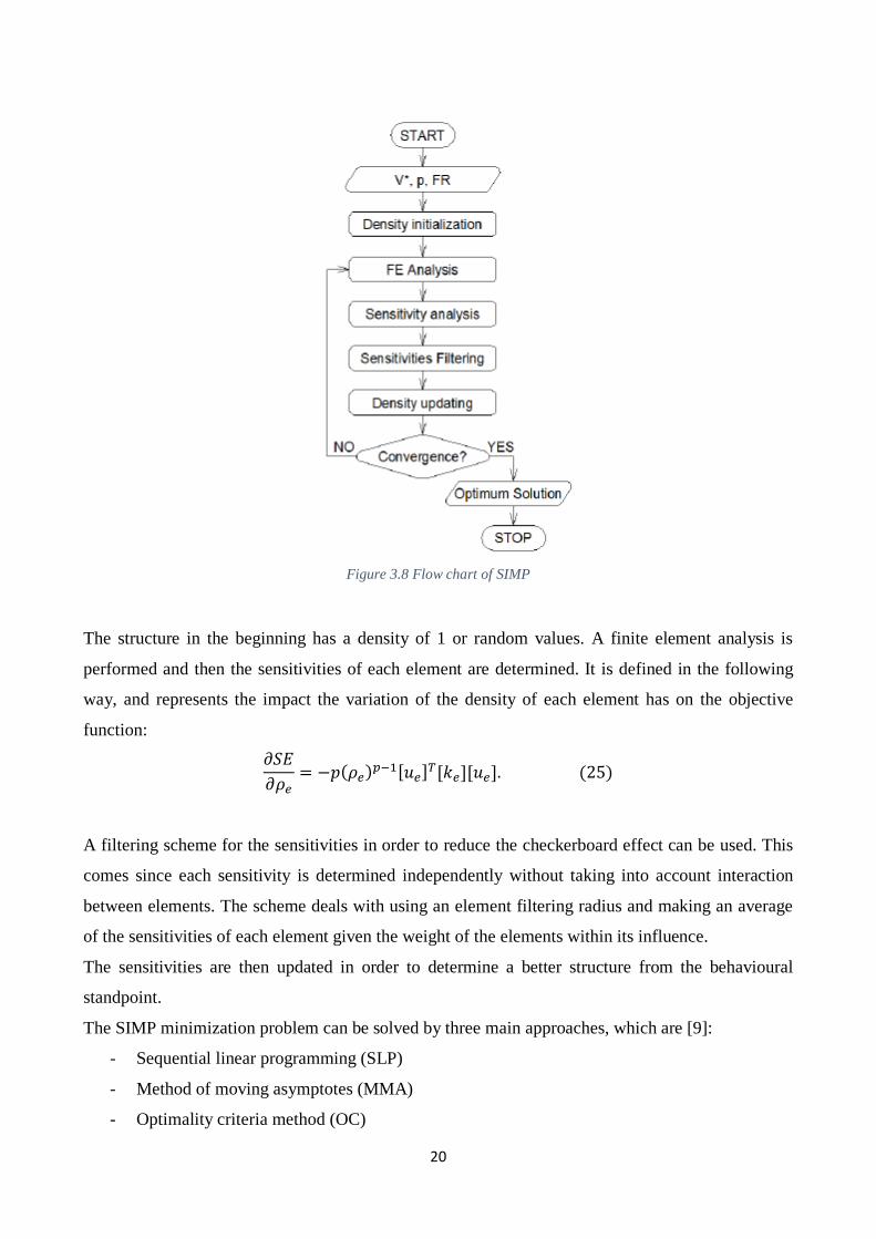
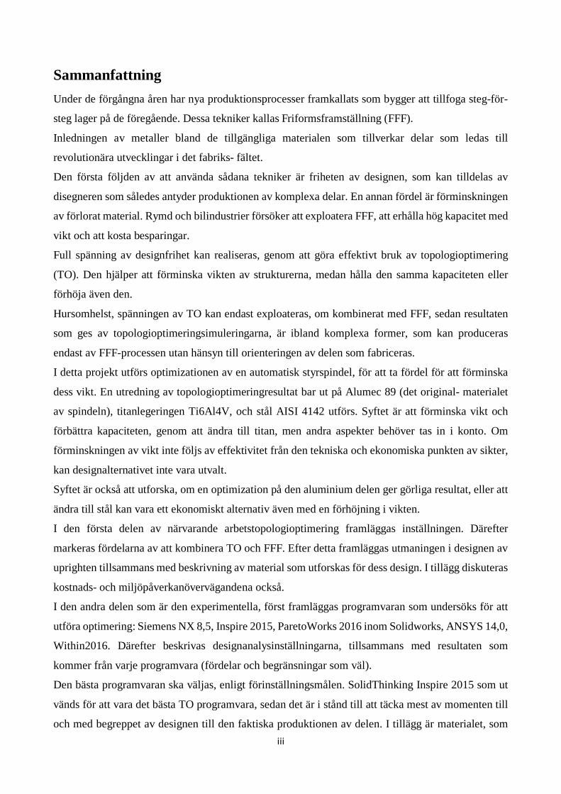
Figure 3.8 Flow chart of SIMP

The structure in the beginning has a density of 1 or random values. A finite element analysis is

performed and then the sensitivities of each element are determined. It is defined in the following

way, and represents the impact the variation of the density of each element has on the objective

function: 𝜕𝜕𝑆𝑆𝐸𝐸𝜕𝜕𝜌𝜌𝑟𝑟

= −𝑝𝑝(𝜌𝜌𝑟𝑟)𝑝𝑝−1[𝑢𝑢𝑟𝑟]𝑇𝑇[𝑘𝑘𝑟𝑟][𝑢𝑢𝑟𝑟]. (25)

A filtering scheme for the sensitivities in order to reduce the checkerboard effect can be used. This

comes since each sensitivity is determined independently without taking into account interaction

between elements. The scheme deals with using an element filtering radius and making an average

of the sensitivities of each element given the weight of the elements within its influence.

The sensitivities are then updated in order to determine a better structure from the behavioural

standpoint.

The SIMP minimization problem can be solved by three main approaches, which are [9]:

- Sequential linear programming (SLP)

- Method of moving asymptotes (MMA)

- Optimality criteria method (OC)

20

The problem can be solved in this way in an efficient way since the number of active constraints is

usually small, even though the number of variables is large [10].

A problem related to SIMP method is mesh dependency [8].

Usually a fine mesh yields a large number of excessively thin members, thus affecting the

manufacturability of the optimized structure. This is due to the ill-posedness of the generalized

physical description of the problem, thus causing nonexistence of solutions.

Figure 3.9 Mesh dependency example for SIMP

An example of this issue is shown in figure 3.9, where the same problem is solved with two different

solutions. The first is discretized by a mesh of 30x60 unit square elements, whilst the second one

60x120 elements of length 0.5. The finer mesh produces more members, which are in some cases

narrow. Perimeters constraints can reduce mesh dependency.

3.3.3 Problems related to post processing within topology optimization

Topology optimization implies many steps in order to obtain the final optimized component, which

will be later manufactured, even after the simulation process.

In fact, everything starts with the definition of the solver and the method used to run the optimization

process. After that, it is possible to apply loads and constraints on the model, step followed by the

definition of the settings required for the optimization simulation in order to reach the predefined

objectives.

21

After the simulation is done and the optimized results are available, further work is required. Actually

post processing is needed for the optimized component, because a uniform density structure is the

only accepted in order to get a component which is actually both manufacturable and usable [11].

It is for example necessary to avoid situations such as the one shown in figure 3.10:

Figure 3.10 Situation to avoid

It is actually a component likely to be fabricated using AM, however its parts are disconnected from

each other, thus making this result infeasible.

That is why a smooth shape must be interpreted from the topology results, trying to be as close as

possible to the actual optimized shape while respecting the objectives reached through the

optimization process.

This is a work that must be accomplished manually iteratively. This takes a long time, but it is

essential for getting an optimal solution.

In fact, if the part is not perfect to be printed and must be modified, the usual output format given by

an optimization software is .stl, and that is not possible to handle for importing it into a CAD software

in order to make modifications.

Therefore, the original CAD model must be used in order to reach the desired objectives.

22

However, a problem deriving from a manual post processing is the difference on the results coming

from the analysis which is run on the modified component rather than on the original optimized item

[11].

3.3.4 Correlation between topology optimization and additive manufacturing

Recently topology optimization has become an important tool to develop new designs in aircraft and

automobile industries [12]. This allows to get innovative proposals independent of the designer’s

experience.

In the present work, Topology Optimization is meant to be used with Additive Manufacturing in order

to take the best from both.

In fact, as for example demonstrated in [13], the synergistic effect of topology optimization and

additive manufacturing can lead to increase the performance of a component and at the same time

reduce costs and waste of material.

An example of the benefits likely being reached from this way of proceeding can be found in the

aerospace industry, where weight and costs savings are fundamental: there has been a weight saving

of over 1000 kg for the Airbus A380, an important result for the practicality of the aircraft.

The challenge of this project is to reach this goal even with a change in the used material, that is from

Alumec 89 to Ti6Al4V. The advantages of switching to a titanium alloys are presented in chapter 3.

This decision has been made to overcome some difficulties deriving from the use of traditional

subtractive or formative processes and the use of topology optimization within them. In fact, there

are too many constraints that need to be taken into account by using conventional techniques that the

benefit of the optimization are not fully exploited.

Apart from these reasons, also a waste of material has to be avoided.

As for the choice of material, titanium can be used in a relatively easy way within AM instead of

traditional manufacturing methods. This is because of its material properties, which are presented in

chapter 4. Among these, there is the high melting point (close to 1680°C) and high chemical reactivity

at temperature close to the melting point, thus causing problems for forging and machining. Also,

casting is difficult to use since titanium has a high reactivity with most mould materials along with

strong relationship between dissolved gases and its strength and ductility.

23

The use of AM simplifies also the possibility to produce complex and customized geometries, since

it does not deal with subtracting or forging material.

Nowadays most commercial FEA software include capabilities of topology optimization, with Altair

being a company which gave a lot of effort in order to reach important results [10].

However, they are mainly addressed to the use of AM since the results provided by these software

are really complex thus making it quite impossible to be manufactured by traditional techniques. For

example, for a part to be feasible for casting cavities need to be open and lined up with the sliding

direction of the dies. This is not always possible with topology optimization.

In order to satisfy constraints for traditional techniques, software have to be equipped with related

settings.

An interesting use of AM with TO is in medical applications, since this combination allows for

producing latticed or cellular structures, or even single structures with non-homogenous densities.

This way it is possible to design parts with properties similar to bones or organic material being

supported or replaced.

24

4. APPLICATION OF TOPOLOGY OPTIMIZATION

4.1 Case study

This work is carried out in collaboration with the Formula Student, that manufacture every year a

racing car to compete in the annual competition among universities all over Europe.

The case study of the present work is a front upright, with the aim to reach important results as

particularly in automotive and aerospace industry is happening. For such competitions is in fact really

important to reach high speed and, in order to obtain the maximum speed the weight must be the

minimum. That is why the designer needs to design components in such a way that the weight is

reduced as much as possible while they are suitable to sustain maximum stress and force. Not only,

this way of acting can also bring to increase heat dissipating properties [14].

This component is in charge of link together different parts of the racing car. In figure 4.1 and 4.2 the

upright as fabricated and mounted for the 2016 competition is shown:

Figure 4.1 2016 Competition Upright, overview 1

25

Figure 4.2 2016 Competition Upright, overview 2

It is actually a component playing an important role in the suspension unit as an upright supports parts

of the suspension system and creates a link between the wheel, that is tire, rim, brake, disc, hub, and

the suspension system, that is upper and lower wishbones, push rod arms and steering arm. There is

also a connection with the brake calliper. It must move through a wide range of motion without

interference [15].

It is considered as unsuspended component, although it has to support very high stresses.

The case where this happens is when the wheels are fully turned [14]. In particular, the most stressed

upright is the outer one.

26

4.1.1 Geometry of the upright

In figure 4.3 a representation of the upright via a CAD model follows. The main connections with

other components of the car are also highlighted.

Figure 4.3 Geometry and connections of the upright

The dimensions of the upright are the following:

• Height = 264.34 mm

• Width = 145.4 mm

• Depth = 40 mm

The weight of the model, built in aluminium, is about 0.6 kg with the original material, Alumec 89.

27

4.1.2 Stress analysis

Different load scenarios occur during the operation of a car. Among them, there are: linear

acceleration, braking performance, steady state cornering, and linear acceleration with cornering and

braking with cornering [16].

In this work the topology optimization is performed according to the two worst loading cases, which

are:

• 1g in braking and 1g in cornering

• 5g in bumping

The calculation of the loads was done in a simplified way. In fact, starting from the forces exchanged

between the wheels and the road and knowing the arm between the application point of them and the

application point of the reaction forces on the bearing seats, it is possible to obtain sufficiently

approximated values of the loads acting on the upright. The aim is actually to calculate forces and

moments and torque acting on the bearing seats.

It must be then stated that because of this it is necessary to define some surfaces of the upright as

non-design one. In fact, if they were removed some important connections with other components

would be erased, thus creating obstacles for the workability of the car.

Non-design space is defined as a space which is not involved in the simulation within an optimization

software. In this way, fundamental parts of a component are kept which allow junction or interaction

with other items.

Moreover, this simplification leads to possible numerical errors in the calculation of the key values

(stress, displacement). However, difficulties in determining the actual loads acting on the upright

occur, that is why this way is yet accepted.

1g braking and 1g cornering

This is a complex scenario, but really likely to occur. There is the presence of forces in all three

directions both in the front and in the rear of the vehicle.

The assumption is that the car is turning on the left, so the most stressed wheel is the front right one.

The focus will be hence on it.

28

As for the reference system, it is assumed that the positive x direction is from the rear to the front, the

y direction from the right to the left. Therefore, z direction points upwards.

Figure 4.4 Reference system for the loads calculation

Fx is due to the forces generated by deceleration, in fact there is a weight transfer of rear to front of

the vehicle caused by the braking.

As for the forces on y direction, there is a shift of forces and weight from the left to the right, as

known. This is caused due to the centripetal force, whose value is

𝐹𝐹𝑦𝑦 =𝑚𝑚 𝑣𝑣2

𝑟𝑟 , (26)

Where m is the mass of the object, v is the tangential speed along a path with radius of curvature r.

In a real case scenario, the radius of the turn and the velocity are variables, however in this case it is

assumed that the velocity and lateral acceleration are constant while the radius of the turn is calculated

through equation (26).

The force Fz is determined from the roll moment, as shown in equation 27:

29

𝑀𝑀′ɸ𝑟𝑟 = 𝐾𝐾ɸ𝑟𝑟

𝑊𝑊ℎ1𝑉𝑉2𝑅𝑅𝑅𝑅�

𝐾𝐾ɸ𝑟𝑟 + 𝐾𝐾ɸ𝑟𝑟 −𝑊𝑊ℎ1+𝑊𝑊𝑟𝑟ℎ𝑟𝑟𝑉𝑉2

𝑅𝑅𝑅𝑅 = 𝛥𝛥𝛥𝛥𝑧𝑧𝑟𝑟𝑡𝑡𝑟𝑟, (27)

Where:

• 𝛥𝛥𝛥𝛥𝑧𝑧𝑟𝑟𝑡𝑡𝑟𝑟 = 𝛥𝛥𝑧𝑧𝑟𝑟0 −𝑊𝑊𝑟𝑟

2� = −�𝐹𝐹𝑧𝑧𝑟𝑟𝑖𝑖 −𝑊𝑊𝑟𝑟

2� �

• ℎ1 is the height from roll axis to the centre of gravity of the vehicle [mm]

• ℎ𝑟𝑟 is the roll centre height with respect to front axle [mm]

• 𝑡𝑡𝑟𝑟 is the front track width [mm]

• 𝐾𝐾ɸ𝑟𝑟,𝑟𝑟 is the roll stiffness of the suspension rear,front [Nm/deg]

The roll stiffness of the suspension is the roll resisting moment which is caused by the lateral

separation between the springs:

𝐾𝐾ɸ = 0.5𝐾𝐾𝑠𝑠𝑠𝑠2, (28)

where

- 𝐾𝐾𝑠𝑠 is the vertical rate of each of the left and right springs [N/mm]

- 𝑠𝑠 is the lateral separation between the springs [mm]

So it is possible to understand that the force is a function of vehicle weight, roll axis height, track

width, the roll stiffness of the suspension, the velocity of the car and the radius of the turn.

The forces in the y direction react in the same direction for the inside and the outside tires. So the

reaction forces are added to Fy acting on the centre of gravity. Therefore a moment is generated with

the moment arm which is the height of the centre of gravity.

The expression of the roll moment is equal to the total change in Fz times the track width of the

vehicle. Afterwards the total change in Fz is split between the outside and the inside tires. As for the

force on the outside tire, it will be equal to the roll moment plus the weight on the front tires divided

by two.

As for the braking force Fx, it is equal to the weight on the wheel (static minus dynamic according to

the outside wheel) multiplied by the traction limited coefficient of friction.

The values of the forces are the following:

Fx = -1000 N

Fy = 800 N

Fz = 1000 N

30

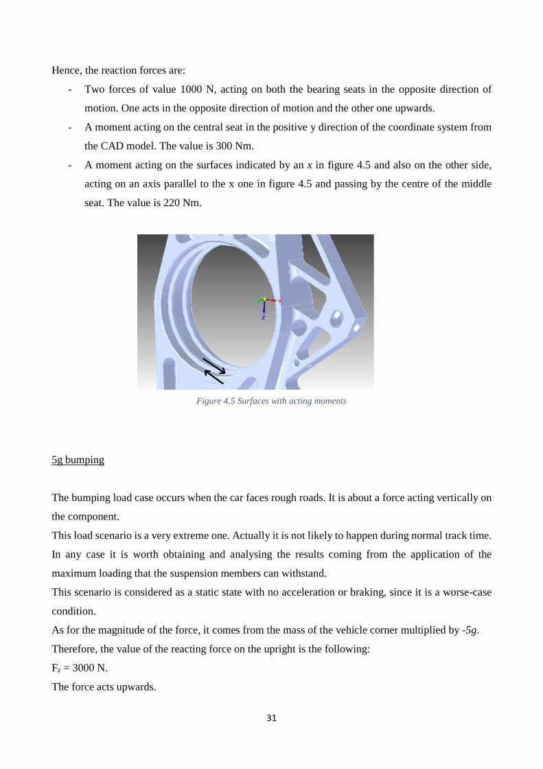
Hence, the reaction forces are:

- Two forces of value 1000 N, acting on both the bearing seats in the opposite direction of

motion. One acts in the opposite direction of motion and the other one upwards.

- A moment acting on the central seat in the positive y direction of the coordinate system from

the CAD model. The value is 300 Nm.

- A moment acting on the surfaces indicated by an x in figure 4.5 and also on the other side,

acting on an axis parallel to the x one in figure 4.5 and passing by the centre of the middle

seat. The value is 220 Nm.

Figure 4.5 Surfaces with acting moments

5g bumping

The bumping load case occurs when the car faces rough roads. It is about a force acting vertically on

the component.

This load scenario is a very extreme one. Actually it is not likely to happen during normal track time.

In any case it is worth obtaining and analysing the results coming from the application of the

maximum loading that the suspension members can withstand.

This scenario is considered as a static state with no acceleration or braking, since it is a worse-case

condition.

As for the magnitude of the force, it comes from the mass of the vehicle corner multiplied by -5g.

Therefore, the value of the reacting force on the upright is the following:

Fz = 3000 N.

The force acts upwards.

31

4.2 Challenge: switching from aluminium to titanium. Possible risks. Investigation of optimization with aluminium and steel as well In this work a challenge is faced. In fact the will is to switch the material used to fabricate the upright

from the actual aluminium to titanium.

The motivation behind the choice of trying to use a titanium alloy for producing the upright is that a

stiffer material is investigated as new one for the item with the aim of reducing the weight of the

component at the same time.

A comparison between the two materials can be presented, describing important properties according

to [17] [18].

Aluminium is the third most abundant element in Earth’s crust, while titanium is the ninth.

Aluminium is a malleable metal and lightweight: its density is 2700 kg/m3 (circa one-third that of

steel), while titanium, which has a high strength to weight ratio (it is actually the highest of any metal

on Earth) and is quite ductile in an oxygen free environment, is a transition metal whose density is

4507 kg/m3 (approximately 60% more than that of aluminium). This is an important property since

in many applications aluminium is rather preferred instead of using even steel (between 7500 and

8000 kg/m3), in particular for fabricating aircrafts.

However, titanium is characterized by a very high melting point (circa 1680°C), which makes it

suitable as refractory metal. Moreover, it has low thermal and electrical conductivity and is

paramagnetic, whilst aluminium is not magnetic.

Titanium has also double the strength of aluminium, 6 versus 2.75 (according to the Mohs scale of

mineral hardness).

Another characteristic about titanium is that it can dampen vibration thus decreasing the amount of

vibration transmitted to the user, while aluminium is easy to be bent and welded.

Compared to aluminium, in addition, titanium has an incredible durability and it does not rust or

corrode in any atmospheric environment. It also never shows signs of wear whilst other metals start

to fatigue with repetitive use.

The cost of titanium is higher because it is difficult to refine and process, while aluminium is typically

cheaper.

So, another reason for topology optimization being exploited can be noticed.

Sometimes, it is in fact preferred having a heavy suspension system, since the performance gained by

reaching a heavier but stiff suspension is more important than a lighter car [15]. 32

But, what if it would be possible to switch from aluminium to an even heavier material, in this case

titanium, in order to get better performance and also reduce weight?

However, in order to do so, optimization simulations need to be run to reduce the quantity of material

needed to support the structure.

The challenge is therefore trying to reduce the weight even with this material change.

However, a business evaluation needs to be made as well. In fact, as stated in chapter 5, the price per

kg of the materials has to be taken into account. That is why also steel is considered in this analysis.

Even if its density is higher than both Alumec 89 and Ti6Al4V, it is definitely cheaper, so an analysis

considering both the weight and the cost of material will be made.

33

4.3 Research questions

After presenting the challenge faced, it is possible to define the research questions.

They actually clarify what the aims of the present work are.

These questions, after the description of the literary background and the numerical section, are going

to be answered in the result chapter.

1) Is it possible to use a reliable topology optimization software or they are still on the way of

improving themselves? That means, what are the limitations faced in each software and do

they allow applying all the possible scenarios required?

2) Is it possible to perform topology optimization on the component used in this work by getting

reliable results, since it has a complex shape?

3) Is it feasible to switch from Alumec 89 to Ti6Al4V for manufacturing the upright from the

manufacturing and economical standpoint? Or is it better to use steel (AISI 4142 in this case)

or keep aluminium?

34

5. MATERIAL DESCRIPTION

5.1 Titanium: description of properties and application in additive manufacturing

Titanium is a material whose use has been sought thanks to its appeal to the aerospace industry and

other sectors where high performance is required [13]. In addition, also the synergistic effect of AM

and TO is exploited in many cases as the TiLight project [19], including this work, in order to increase

the performance of the component while reducing costs and waste of material.

Titanium and its alloys are used in some applications, including aerospace, mainly due to their low

weight (compared to some materials), high specific strength, high creep strength and corrosion

resistance. For example, titanium alloys are circa 60% heavier than aluminium alloys but have almost

double the strength (strength being even higher than steel) [13].

There are different titanium grades, which are used instead of pure titanium since the latter is not as

strong as the titanium alloys.

In this work Ti6Al4V is the reference alloy, which is also the most widely used, thanks to its good

machinability and mechanical properties [20].

If the component is subject to fatigue loads, a heat treatment is recommended: Hot Isostatic Pressing

(HIP).

In any case fatigue is not considered in this work, since the car will not race for long time. This

implies that the upright will not be stressed for many cycles (that is also why the loads are calculated

in an easier way, see chapter 4. There is in fact no need to consider dynamics loads).

Some problems deriving from the use of titanium as material for many applications is for example

the high melting point (1680°C) and high chemical reactivity at temperatures close to melting point.

That is why conventional manufacturing processes like forging and machining are hard to control.

Or, casting techniques are difficult to handle because of the high reactivity with most mould materials

and the relationship between the content of dissolved gases and the material strength and ductility.

Hence some constraints must be taken, which are not advantageous for the component being produced

[13]. An example is the so called electromagnetic constraint forming technique for casting. It helps

35

reduce many problems such as contamination of titanium alloys along with ingredient segregation,

microstructure coarsening, poor performance because of the high melting point. However, some

problems are still to be resolved in controlling the forming and properties.

To conclude, this is the chemical composition of the alloy:

Substance Concentration (%)

C <0.08

Fe <0.25

N2 <0.05

O2 <0.2

Al 5.5-6.76

V 3.5-4.5

H2 <0.015

Ti Balance

The price per kg such a quality alloy is about $200.

5.2 Alumec 89

Alumec 89 is a high strength aluminium alloy [21].

It is widely used in the manufacturing industry thanks to its high strength and good stability.

Its chemical composition is the following (concentrations in %):

Substance Concentration (%)

Aluminium > 84

Zinc <12

Magnesium <3.7

Copper <3.3

Cobalt <2

Manganese <1.5

Iron <1.4

36

Silicon <1.2

Chromium <0.4

Nickel 0 – 0.2

Lead <0.05

The major properties of the alloy, used in this work, are the following:

Density Elastic modulus Poisson’s ratio Yield stress Price

2830 kg/ m3 71.5 GPa 0.33 480 MPa 60 $/kg

5.3 Steel AISI 4142

Steel AISI 4142 is an alloy steel.

Its chemical composition is the following (in %):

Fe Cr Mn C Si Mo S P

≥ 96.725 0.80 –

1.10

0.75 –

1.10

0.40 –

0.45

0.15 –

0.30

0.15 –

0.25 ≤ 0.040 ≤ 0.035

The major properties, used in this work, are the following:

Density Elastic modulus Poisson’s ratio Yield stress Price

7870 kg/ m3 200 GPa 0.29 585 MPa 12 $/kg

37

6. BUSINESS CONSIDERATION

In this chapter a business consideration on the use of Additive Manufacturing for producing the parts

is taken into account. In fact only a profitable way of producing can be accepted and introduced by

the manufacturers as a common technique within the industry.

The factors associated with manufacturing which must be considered for such an analysis are the

following:

1. Fixed or nonrecurring manufacturing costs, which include tools, dies, buildings and so on.

These are amortized over the number of items produced.

2. Recurring costs, which are expenses for material, labor and so on. So they mostly depend on

the produced part.

An example can be presented according to [20]. In figure 6.1 a comparison between the cost of

producing parts via Additive Manufacturing and conventional techniques is presented.

Figure 6.1 Comparison between costs due to AM and conventional techniques

There are two assumptions to be considered for this example, that is the fixed costs of conventional

manufacturing process are ten times higher than the ones of Additive Manufacturing, and two cases

of Additive Manufacturing are taken into account, where the recurring costs are higher by 1.5 and 2

times.

The total cost is dependent on the number of parts which are produced (represented on the x axis).

38

As for the y intercept, it represents the value of the fixed cost for each technique. Finally, the slope

of the lines corresponds to the ratio of the recurring cost of technique taken into account divided by

the recurring cost of conventional manufacturing.

As previously stated, conventional processes imply higher fixed costs since they involve operations

such as metal working and machining. On the other hand, the recurring costs are lower than in AM.

An example can be about the raw materials, much more expensive in AM, even though some attempts

are on the way to get cheaper raw materials, for example directly from the ore for titanium alloys

[22].

This explains why conventional techniques are more effective for large production lots.

At the cross-over point, instead, the choice between one process or the other is indifferent, since they

have the same costs.

There is instead a great interest for AM in small production lots, as the reduction in fixed costs would

compensate the increase in the cost of raw materials for AM. In customisation, for example, AM has

to be seriously taken into account since it allows to produce small batches of products implying fewer

risks. [23]

There are other factors which must be considered apart from recurring and nonrecurring costs for this

comparison. The first ones are the versatility, adaptability and speed of AM. In fact there would be a

huge interest in a process which gives the possibility to produce critical parts in days instead of weeks.

So these should be taken into account even though there is no possibility to quantify this opportunity.

These factors can be identified as [23]:

• Freedom of design

• Reduced time-to-market

• Maintenance of the machine is faster and easier

• Tooling costs are dramatically reduced

• Assembly time is decreased since there is the possibility to print parts in one go, without

focusing on sub-assembly.

The second factor to consider is the potential for AM to reduce the logistical cost and energy related

to the packaging, transport and storage of spare parts.

Another problem in the present consideration must be pointed out.

In fact, the choice of the material to use for printing a component has to be also based on the

convenience coming from the cost of the material itself.

39

That means that maybe one material has better performance compared to another one and is more

suitable, but if its price per kg is higher and the weight is not low enough such that the total cost

coming from the use of material can justify the choice of the material, then another way should be

taken.

In this work Alumec 89, Ti6Al4V and Steel AISI 4142 are investigated.

The properties of each material has been presented in chapter 4.

The prices of the materials are the following:

• Alumec 89: 8 $/kg

• Ti6Al4V: 15-40 $/kg

• Steel AISI 4142: 1-3 $/kg

So the choice of switching material from Alumec to titanium needs to be justified also from the

economical point of view.

The weight reached by topology optimization on titanium component should be low enough in order

to consider the material as the new one for the upright.

Or it could be even more advantageous to switch to steel, since it is more widespread than aluminium

alloys, which means that it is cheaper.

In chapter 8, where the results are presented, a consideration taking into account even the price of

material is done.

40

7. ENVIRONMENTAL IMPACT FROM USING ADDITIVE MANUFACTURING

One of the problems faced nowadays is that the way mankind is exploiting Earth is far more than its

long-term capacity, the scientists say [24].

That is why it is important to focus also on the environmental impact provided by Additive

Manufacturing (and the results which can be reached through the exploitation of topology

optimization) and compare it afterwards with the one related to traditional processes.

In fact, it can be another discriminating factor guiding the manufacturers to choose a manufacturing

technique instead of another.

Life-cycle assessment is an approach for determining the Environmental Impact originating from the

inputs and outputs related to a product’s life cycle.

It is a standardized approach and divided into three steps [25]. They are the following:

• Description of the product, process or activity to analyse as well as the boundary conditions

to consider.

• Introduction of the inputs (energy, material, fluids) and the outputs created (waste, emissions).

• Determining the consequences of the inputs and outputs on human health and ecosystem.

The aim of this analysis is actually to understand if it is possible to reduce the Environmental Impact

(E. I.) by exploiting powder bed fusion (PBF) processes in the industry.

Some results were found by many researchers and some of them are here presented, however there

are still unresolved issues because of the scarsity of research and the rapid evolution of the technology

[20].

One experiment was performed by Morrow et al., comparing the impact of laser-based AM and

conventional processes for fabrication of tools and dies. Environmental impact and cost was proved

to be better for laser-based processes.

An experiment giving a warning about this kind of analysis comes from Kellens et al., who examined

the energy efficiencies of the SLS and SLM. The problem was that the information regarding energy

consumption, waste flows and emissions is often lacking.

41

One of the benefits of using AM processes is the cost savings regarding electric consumption [24].

Conventional techniques are more energy intensive than AM systems. The latters in fact only require

a single machine using a beam or a deposition nozzle. Some values can be seen in figure 7.1.

Figure 7.1 Environmental impact of conventional and innovative techniques

Waste is generated by both ways of fabricating parts: subtractive methods produce chips, which could

even be recycled; AM processes use for the parts only the required material, but sometimes it is

necessary to generate supports thus wasting powder. However, now it is possible to reuse almost all

the powder unused from the process.

Moreover, since a single machine operating AM can handle a great variety of designs and print more

parts at the same time, it is then suitable to act in the distributed manufacturing, thus allowing a

production location at the optimum distance between the material resource and the customers. This

implies less packaging and transportation, so there is a decrease in energy consumption and air

emissions [20].

However, some aspects need to be taken into account [26]. As for the electrical consumption, for

example, it is directly dependent on the duration of the job. The manufacturing time is the most

42

important factor, along with the cooling and heating. So it is difficult to prescribe a specific energy

consumption constant for the processes because of the variance in build density and height.

Another problem to consider is related to material toxicity. It is on the way a study about the

toxicological and environmental risks resulting from handling, using and disposing of the materials

which are used in AM methods.

In any case, there is a great potential provided by AM in reducing the carbon emissions, which comes

from the exploitation of design optimization thus resulting in reduction of material waste. In fact

optimization can even bring to a weight saving of about 40%. And in the aerospace field, for example,

a weight saving on an aircraft of 100 kg can provide a 2.5 million dollars saving in fuel and a 1.3

MtCO2 savings over the lifetime of it [20].

This explains why more research needs to be done in order to investigate the impact of AM on the

environment.

43

8. NUMERICAL SECTION

In this chapter all the chosen software are analysed. This in order to understand what the possibilities

and the limitations provided by each of them are. The order used is the following:

• ANSYS Mechanical 14.0

• solidThinking Inspire 2015

• Siemens NX 8.5

• ParetoWorks 2016

• Autodesk Within 2016

In particular, the analysis has been performed for the following aspects:

• The steps to create a new file

• The application of constraints and loads

• Definition of the settings for the optimization simulations

• Analysis of the optimized results (where relevant)

8.1 ANSYS Mechanical 14.0

ANSYS Inc. is a company established in 1970 and develops finite element software in several fields

of engineering [27].

In ANSYS Mechanical it is possible to perform several type of analyses, including structural analysis

and design optimization of the components.

This is provided by the use of Workbench, a platform integrating the different simulating tools within

ANSYS packages.

The module used in this case in a pre-installed plug-in, Shape Optimization (Beta), which is possible

to obtain by the settings in Workbench.

It was possible to apply the braking and cornering scenario. However, there was no possibility to

retain some surfaces, which are needed for being in contact with other components.

That is the reason why the software was discarded.

44

The setting of the loads and constraints application follows along with the definition of the

optimization simulation.

Simulation procedure

First of all it is necessary to open Workbench. After that one can create a new project and import the

part. By selecting

FileImport

it is possible to import the upright model in step format.

If one wants to run an analysis before optimizing the component, Static Structural has to be selected

from the list on the Analysis System list on the left of the screen and dragged onto the work window.

Afterwards, the Shape Optimization (Beta) module needs to be dragged into the main work window,

close to the Geometry module.

Then, the geometry must be linked to the one included in the modules. It is accomplished by clicking

on Geometry from geometry window and dragging it onto the same name from Static Structural and

Shape Optimization box.

Double clicking on Model it is possible to open Mechanical.

In figure 8.1 it is possible to see the result of these steps within Workbench.

Figure 8.1 Workbench screen after the definition steps

45

Before starting, a coarse mesh, with default size of elements was chosen.

In Mechanical it is then possible to apply at first the constraints.

In order to do so, Fixed support is applied to the required surfaces, as shown is figures 8.2, 8.3, 8.4.

Figure 8.2 Constraints with UCA connection, Ansys 14.0 Figure 8.3 Constraints with steering mechanism, Ansys 14.0

Figure 8.4 Constraints with LCA connection, Ansys 14.0

The issue regarding such constraints, is that it is not possible to define in which direction to lock the

motion of the component. Therefore, it is locked in all directions.

In order to solve this problem, displacements were defined as free in the directions which are not

supposed to be locked. They are: z direction in the LCA connection and x and y in the steering

mechanism connection.

Applying the loads is the following step.

A moment is applied on the middle cylindrical surface between the bearing seats. It is important to

select Define ByVector and the positive y direction.

46

A moment is applied on the bearing seats and the vertical surfaces close to them along an axis passing

by the middle of the central seat of the upright and the centre of the cylindrical surfaces, in the positive

x direction. The definition is the same as before.

Two forces are applied on the bearing seats, each of them with a value of 1000 N and acting in positive

x and z direction. Figure 8.5 describes how to set the forces.

Figure 8.5 Definition of the forces, Ansys 14.0

In order to define retention of required surfaces, fixed supports were defined on the faces shown in

figures 8.6, 8.7, 8.8, and then a free displacement set for the motion of the component.

Figure 8.6 Retaining the shown surface, Ansys 14.0 Figure 8.7 Retaining the shown surface, Ansys 14.0

47

Figure 8.8 Retaining the shown surface, Ansys 14.0

It is the time for running the simulation.

In Solution Shape Finder it is possible to define the target reduction for the upright.

A value of 30% has been chosen.

Right clicking on Shape Finder the Solve command can be found and the simulation can be run.

The results are shown in figure 8.9.

Figure 8.9 Simulation result with Mechanical

It is actually possible to remove material on the upright, getting some important results as well.

However, the non-reliability of the procedure did not allow to consider these results.

48

8.2 SolidThinking Inspire 2015

SolidThinking Inspire 2015 is a software allowing design engineers to create or import concepts and

to investigate them from the structural standpoint [28].

Moreover, it is also possible to run optimization simulations in order to change the topology of the

component. In order to do so, SIMP method is used.

Inspire is actually a simplified version of Hyperworks, a CAE package from Altair Engineering [29].

It works with design and non-design spaces, so in order to perform topology optimization simulations

it is required to split the component under inspection in parts.

In this work attempts were made in order to split the upright in CAD software such as Solid Edge ST7

or Solidworks, but the import of the split part into Inspire was not successful since some parts being

design space were not recognized by the software, and they were actually parts classified as design

space. So an attempt was done directly in the software, and a difficulty in using the Cut command

was found. The main problem is that it was not possible to split the upright in a precise way, so an

approximate procedure was accomplished.

The procedure for running simulations is the same for all the three investigated materials, so only the

steps for the upright in titanium is thoroughly described. The important steps are instead presented

for the other materials.

The braking and cornering scenario is applicable within this software.

It was necessary to define, in material library, the properties of Alumec 89 and Ti6Al4V.

49

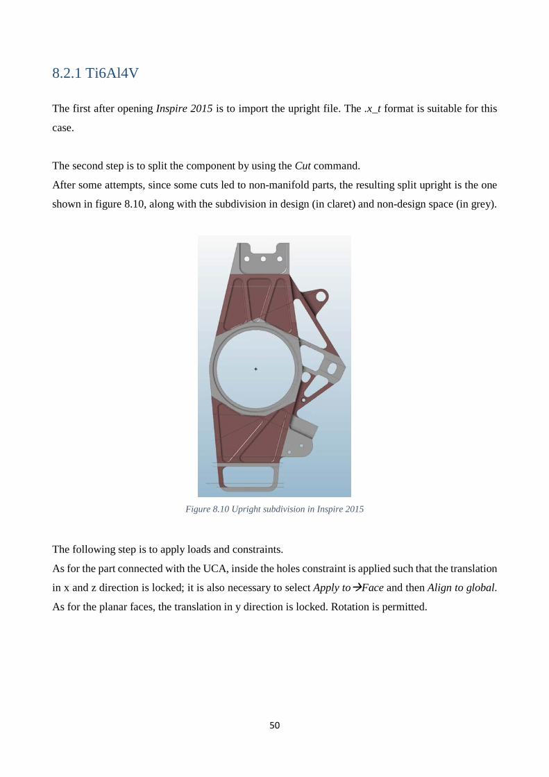
8.2.1 Ti6Al4V

The first after opening Inspire 2015 is to import the upright file. The .x_t format is suitable for this

case.

The second step is to split the component by using the Cut command.

After some attempts, since some cuts led to non-manifold parts, the resulting split upright is the one

shown in figure 8.10, along with the subdivision in design (in claret) and non-design space (in grey).

Figure 8.10 Upright subdivision in Inspire 2015

The following step is to apply loads and constraints.

As for the part connected with the UCA, inside the holes constraint is applied such that the translation

in x and z direction is locked; it is also necessary to select Apply toFace and then Align to global.

As for the planar faces, the translation in y direction is locked. Rotation is permitted.

50

Figure 8.11 Constraint with UCA connection, Inspire 2015

In the section connected with the steering mechanism, still applying the constraint to face, the z

direction translation is locked, whereas the rotation is allowed.

Figure 8.12 Constraints with steering mechanism, Inspire 2015

The DOFs of x and y direction for the holes connected to the LCA are locked. The rotation is

completely free.

51

Figure 8.13 Constraints with LCA connection, Inspire 2015

The application of the loads is a bit time consuming, even though the software allows to apply all the

required loads on the upright.

Two forces are applied on each bearing seat, with value 1000N and acting in the positive x and z

direction. A moment of 300 Nm is applied on the central cylindrical surface of the upright acting on

the positive y direction of the axis of the surface. A moment of 220 Nm acts instead on the bearing

seats and the vertical surfaces close to them along an axis passing by the middle of the central seat of

the upright and the centre of the cylindrical surfaces, in the positive x direction.

Figure 8.14 Loads application, Inspire 2015

It is now possible to optimize the component by selecting the Run Optimization. The objective set in

this software is Maximize Stiffness with a mass target.

After some attempts, for titanium a mass target of 30% of the original design space has been chosen.

The minimum thickness has been varied due to the mesh dependency of the SIMP method used by

52

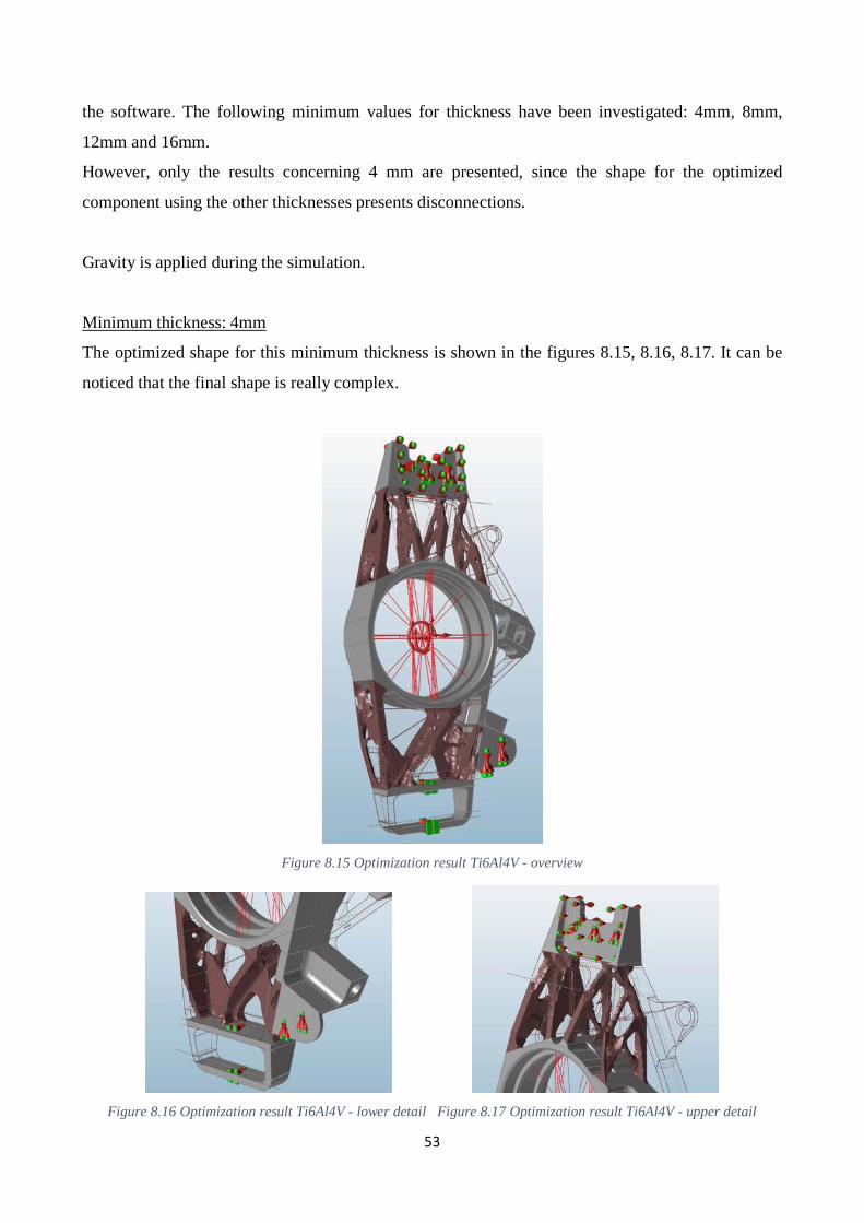
the software. The following minimum values for thickness have been investigated: 4mm, 8mm,

12mm and 16mm.

However, only the results concerning 4 mm are presented, since the shape for the optimized

component using the other thicknesses presents disconnections.

Gravity is applied during the simulation.

Minimum thickness: 4mm

The optimized shape for this minimum thickness is shown in the figures 8.15, 8.16, 8.17. It can be

noticed that the final shape is really complex.

Figure 8.15 Optimization result Ti6Al4V - overview

Figure 8.16 Optimization result Ti6Al4V - lower detail Figure 8.17 Optimization result Ti6Al4V - upper detail

53

The optimized shape can be easily analysed within the software thanks to an integrated solver.

The results are shown in figures 8.18, 8.19, 8.20, 8.21.

Figure 8.18 Displacement results Ti6Al4V

Figure 8.19 Percent of yield results Ti6Al4V

54

Figure 8.20 Von Mises results Ti6Al4V

Figure 8.21 Von Mises results Ti6Al4V - detail

From the figures it can be noticed that the maximum displacement is about 0.29 mm, the maximum

percent of yield is 86 % in a small area and the maximum value for von Mises stress is about 813

MPa. Even though the stress value is extremely high, it is restricted in an area of connection for the

split parts, which were obtained in a step accomplished earlier. Apart from that small region, the

values are far lower and reasonable for manufacturing purposes. This is the reason why this anomaly

can be considered as a numerical error.

The analysis concludes that the optimized shape is acceptable.

The final weight is 0.64005 kg.

55

8.2.2 Alumec 89

In this case, after some attempts, for aluminium a mass target of 35% of the original design space has

been chosen. A higher percentage, let us say 40%, would have created a shape for the optimized

component not possible to manufacture. The minimum thickness has been varied even for this

material. So the following minimum values are evaluated: 4mm, 8mm, 12mm and 16mm.

Only 4 mm gives, however, feasible results.

Minimum thickness: 4mm

The optimized shape for this minimum thickness is shown in the figures 8.22, 8.23, 8.24.

Figure 8.22 Optimization results Alumec 89 - overview

Figure 8.23 Optimization results Alumec 89 - upper detail Figure 8.24 Optimization results Alumec 89 - lower detail

56

The optimized shape is the analysed.

The results are shown in figures 8.25, 8.26, 8.27, 8.28, 8.29, 8.30.

Figure 8.25 Displacement results Alumec 89

Figure 8.26 Percent of yield results Alumec 89

57

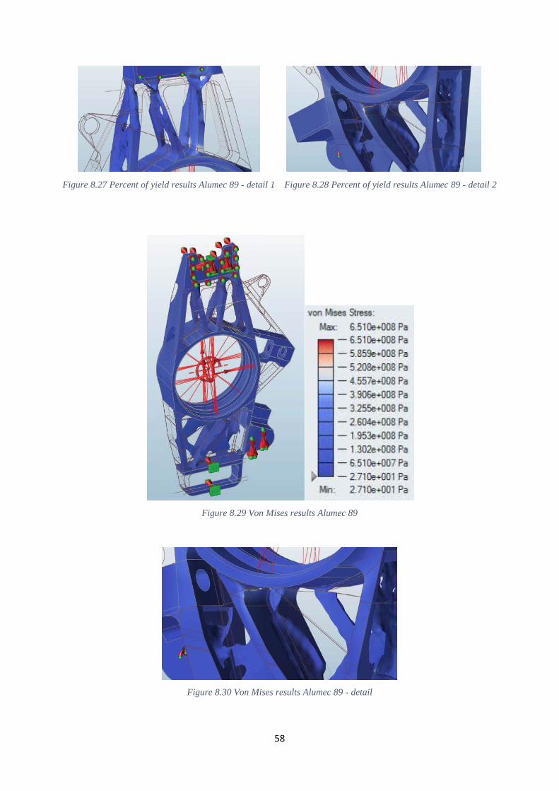
Figure 8.27 Percent of yield results Alumec 89 - detail 1 Figure 8.28 Percent of yield results Alumec 89 - detail 2

Figure 8.29 Von Mises results Alumec 89

Figure 8.30 Von Mises results Alumec 89 - detail

58

From the figures it can be noticed that the maximum displacement is circa1.38 mm; the maximum

percent of yield is 136% in a small area (numerical error due to disconnections of the split parts) and

the maximum value for von Mises stress is 651 MPa in the same area of high percent of yield.

The final weight is 0.42301 kg.

8.2.3 Steel AISI 4142

In this case, after some attempts, for aluminium a mass target of 25% of the original design space has

been chosen. The minimum thickness has been varied even for this material. So the following

minimum values are evaluated: 4mm, 8mm, 12mm and 16mm.

Only 4 mm gives, however, feasible results.

Minimum thickness: 4mm

The optimized shape for this minimum thickness is shown in the figures 8.31, 8.32, 8.33.

Figure 8.31 Optimization results steel AISI 4142 - overview

59

Figure 8.32 (on the left) Optimization results steel AISI 4142 - upper detail

Figure 8.33 (on the right) Optimization results steel AISI 4142 - lower detail

The optimized shape can be easily analysed within the software.

The results are shown in figures 8.34, 8.35, 8.36, 8.37, 8.38.

Figure 8.34 Displacement results steel AISI 4142

60

Figure 8.35 Percent of yield results steel AISI 4142

Figure 8.36 Percent of yield results steel AISI 4142 - detail

61

Figure 8.37 Von Mised stress results steel AISI 4142

Figure 8.38 Von Mised stress results steel AISI 4142 - detail

From the figures it can be noticed that the maximum displacement is circa 0.16 mm, the maximum

percent of yield is 125% in a small area concerning the disconnection of the component (the rest of

the component has percent below 100%) and the maximum value for von Mises stress is 731 MPa (in

the same area).

The final weight is 1.0964 kg.

62

8.3 Siemens NX 8.5

NX 8.5 is a CAD software released by Siemens PLM Software allowing design engineers to use

several tools.

It is actually possible not only to design components, but also, for example, to run structural analysis

on a component created therein or imported.

Aligned with the interest of this work, the software gives also the opportunity to run topology

optimization analysis on the models, thus allowing to reduce their weight by removing material.

In fact, the module included in the software, an add-on to request, uses the SIMP method.

The module is available in a .sim file, linked with the mesh of the model, created in a .fem file. The

mesh is in turn connected to the .prt component file.

The module allows to defining the surfaces to keep or to optimize, thus giving a strong tool to the

designer.

Moreover, in case of conventional manufacturing techniques such as casting, the designer needs to

set constraints related with the specific requirements of the process. However, since AM is considered

here which allows for freedom in design, the step is not considered in this work.

It is possible to apply the braking and cornering scenario thanks to the several loads cases the software

allows to use.

For this software only Ti6Al4V has been investigated, for the reasons later explained.

The file in .x_t format was imported in NX 8.5.

After importing the model, it is saved as default in .prt.

This helps in the next step, which is about creating a .fem file in order to create a mesh for the upright.

Creating a mesh file

In fact, after opening a file with such a format, it is required to link it with the actual model. That is

why the .prt file is fundamental.

63

Figure 8.39 Connection of the .fem file to the .prt file, NX 8.5

In this case two steps need to be carried out, which are assigning material to the component and

meshing it.

As for the material, it is possible to define one if it is missing. For Ti6Al4V this is the way. Then,

clicking on Assign Material the upright can be selected and the titanium alloy can be assigned.

Once the material has been assigned, the mesh is created.

In this case some settings have been defined, which are shown in figure 8.40. They are available by

selecting 3D Tetrahedral.

Figure 8.40 Settings for creating the mesh, NX 8.5

64

It can be noticed that a value of 5 mm for Element Size has been selected. The other values are as

default.

Creating a simulation file

The following step in the procedure is to open a .sim file.

The settings defined in this work are the show in figures 8.41, 8.42.

Figure 8.41 Connection of .sim file to .fem file, NX 8.5

Figure 8.42 Simulation settings, NX 8.5

65

The other options did not change.

After doing that, it is possible to start applying loads and constraints on the upright.

As for the constraints, it is required to select Constraint Type. In this case User Defined Constraint

are used.

In the connection with the UCA the holes are fixed in x and z direction, while the vertical surfaces

are locked in the y direction. The rotations are free.

Figure 8.43 Constraint with UCA connection, NX 8.5

The holes connected with the steering mechanism are locked in z direction. All the DOFs of rotation

are free.

Figure 8.44 Constraint with steering mechanism, NX 8.5

In the connection with the LCA the holes’ DOFs are locked in x and y direction. Rotation is not.

66

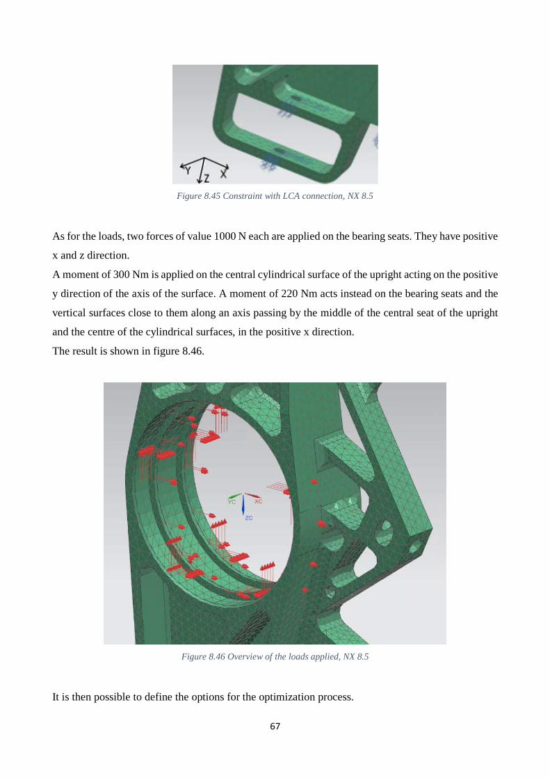
Figure 8.45 Constraint with LCA connection, NX 8.5

As for the loads, two forces of value 1000 N each are applied on the bearing seats. They have positive

x and z direction.

A moment of 300 Nm is applied on the central cylindrical surface of the upright acting on the positive

y direction of the axis of the surface. A moment of 220 Nm acts instead on the bearing seats and the

vertical surfaces close to them along an axis passing by the middle of the central seat of the upright

and the centre of the cylindrical surfaces, in the positive x direction.

The result is shown in figure 8.46.

Figure 8.46 Overview of the loads applied, NX 8.5

It is then possible to define the options for the optimization process.

67

In order to open the topology optimization window, select Insert Topology Optimization.

Many options appear, each of the giving the possibility to run the proper simulation for every case.

In Design Area the area of design and non-design space are defined. For the upright the choice is

shown in figures 8.47 and 8.48 for the design space and 8.49 for the non-design space.

Figure 8.47 Design space - detail 1, NX 8.5

Figure 8.48 Design space - detail 2, NX 8.5

68

Figure 8.49 Non-design space, NX 8.5

The design responses defined for this case are the displacement of a point in the central seat and the

volume.

Figure 8.50 Design responses in NX 8.5

The objective is to minimize the volume with a constraint on the displacement, which needs to be

less than 0.5 mm.

69

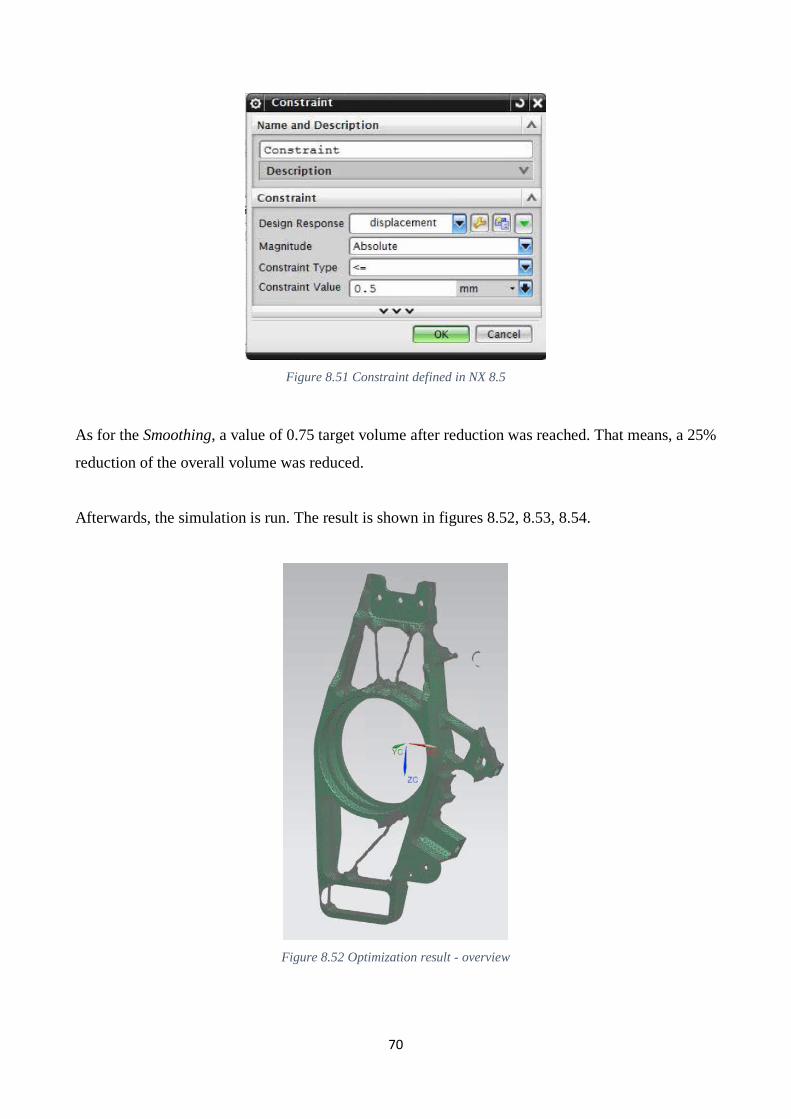
Figure 8.51 Constraint defined in NX 8.5

As for the Smoothing, a value of 0.75 target volume after reduction was reached. That means, a 25%

reduction of the overall volume was reduced.

Afterwards, the simulation is run. The result is shown in figures 8.52, 8.53, 8.54.

Figure 8.52 Optimization result - overview

70

Figure 8.53 Optimization result - detail 1 Figure 8.54 Optimization results - detail 2

The main issue related with this software is that it is not possible to define only the non-design space.

The reason why it is a problem lies in the fact that faces must be selected for the optimization, and

since the upright is a really complex component, it is not possible to define precisely the area where

the material should be removed. So a big amount of material removal is not possible. Moreover, it is

possible to see the disconnection between the material parts after the run.

In addition, some surfaces to be completely kept were affected during the simulation. For example,

on the top contact with the brake calliper, material is removed at the bounds. This occurred since the

surfaces next to it were defined as design space, and that led to removal of the elements close to those

surfaces.

71

8.4 ParetoWorks 2016

Paretoworks 2016 is a free topology optimization plug-in for Solidworks [30].

It was first released in 2013 and was created at University of Winsconsin-Madison.

It is based on level-set method, so it is different from the majority of the contemporary software using

the SIMP method.

It is comfortable to work with it since it is included in a CAD environment, that is Solidworks, so the

import of the files is carried out without any problem.

The procedure for running simulations is the same for all the three investigated materials, so only the

steps for the upright in titanium is thoroughly described. The important steps are instead presented

for the other materials.

Within Paretoworks the bumping scenario is used, since the braking and cornering case presents loads

impossible to apply. They are actually moments acting along axis different from the axis of rotation

of the cylindrical surface where they are applied.

8.4.1 Ti6Al4V

First of all it is necessary to import the upright model. In order to do so, any format compatible with

Solidworks is fine. In this case, a .x_t format was used.

Since the file was provided in that format, which is not actually the one original from the software, a

Feature Recognition needs to be carried out.

After this step, it is necessary to open the plug-in, Paretoworks 2016. In order to do so it is required

to follow this way:

Tools Paretoworks Setup

The screen of Paretoworks appears and it is possible to work on it.

The first step is to initialize the component by defining the material. Figure 8.55 shows the material

definition for this case.

72

Figure 8.55 Initialization in Paretoworks 2016 for Ti6Al4V

The units are Pa for the Young’s modulus and kg/m3 for the density.

Second step is the application of the boundary conditions.

As for the constraints, the DOFs of translation for the holes connected to the UCA are all locked,

while the rotation is allowed.

Figure 8.56 Constraint with UCA connection, Paretoworks 2016

Only the translation in the z direction is locked instead for the hole connected with the steering

mechanism.

73

Figure 8.57 Costraint with steering mechanism connection, Paretoworks 2016

As for the DOFs related to the LCA, the holes were locked in x direction, while the internal surfaces

of the loop are locked in y direction. All the rotations are free.

Figure 8.58 Constraint with LCA connection, Paretoworks 2016

The forces are then applied. Their values is 3000N (bumping scenario acting) in the negative z

direction and are applied to the bearings seats.

74

Figure 8.59 Overview of loads applied, Paretoworks 2016

In this software it is really easy to define the surfaces that must be kept after the optimization process.

After some attempts, all the surfaces which were supposed to be retained were defined. Basically,

they are the ones which must be in contact with other components or were discovered to be retained

in order to avoid some disconnection coming from the optimized material.

Figure 8.60 Surfaces retain overview, Paretoworks 2016

75

Afterwards it is possible to run a Finite Element Analysis. The default value of the number of elements

created during the analysis is kept, which is in this case 143108 elements.

Figure 8.61 FEA settings for Ti6Al4V, Paretoworks 2016

When the FEA is concluded, it allows to performing the optimization simulation. The purpose is to

minimize the volume as much as possible, and a target volume fraction is set as 0.52. This value

comes from a previous simulation, where the minimum percentage of material retained after the

optimization was about 51%. The value of maximum displacement allowed (in mm) is a bit higher

than the value obtained in the analysis of the upright (about 0.4 mm) performed by the vehicle

dynamics team in the Formula Student (set according to their suggestions), while the maximum stress

is considered as the yield strength (in MPa).

Figure 8.62 Topology optimization simulation settings for Ti6Al4V, Paretoworks 2016

The results of the optimization process are shown in the following figures. It was actually possible to

reduce the weight up to 52% of the starting value, obtaining sometimes shapes otherwise impossible

76

to create within a CAD software. And these complex shapes are suitable to produce for additive

manufacturing.

Figure 8.63 Optimization results – overview Figure 8.64 Optimization results - detail 1

Figure 8.65 Optimization results - detail 2 Figure 8.66 Optimization results - detail 3

Running an analysis on the optimized component stress and displacement are found.

Stress analysis reveals that the values are fine with this scenario, and so happens with the

displacement, the maximum values being 73.6 Mpa circa for the maximum von Mises stress and

0.0692 mm for the maximum displacement. 77

Figure 8.67 Von Mises stress results Ti6Al4V

Figure 8.68 Displacement results Ti6Al4V

78

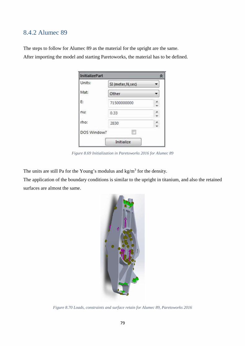
8.4.2 Alumec 89

The steps to follow for Alumec 89 as the material for the upright are the same.

After importing the model and starting Paretoworks, the material has to be defined.

Figure 8.69 Initialization in Paretoworks 2016 for Alumec 89

The units are still Pa for the Young’s modulus and kg/m3 for the density.

The application of the boundary conditions is similar to the upright in titanium, and also the retained

surfaces are almost the same.

Figure 8.70 Loads, constraints and surface retain for Alumec 89, Paretoworks 2016

79

A Finite Element Analysis is then performed. The default value of the number of elements created

during the analysis is kept, which is in this case 143108 elements.

Figure 8.71 FEA settings for Alumec 89, Paretoworks 2016

When the FEA is concluded, it allows to perform the optimization simulation. The purpose is to

minimize the volume as much as possible, and a target volume fraction is set as 0.6. This value is

changed from previous 0.5 to get better shape. Still, the value of maximum displacement allowed is

the same as chosen for titanium (in mm), while the value for the maximum stress is equal to the yield

stress (in MPa).

Figure 8.72 Topology optimization simulation settings for Alumec 89, Paretoworks 2016

The results of the optimization process are shown in the following figures. Even for this material it is

possible to reach the objective and the resulting shape is really complex.

80

Figure 8.73 Optimization results - overview

Figure 8.74 Optimization results - detail 1 Figure 8.75 Optimization results - detail 2

Running an analysis on the optimized component, stress and displacement are found.

Stress analysis reveals that the values are fine with this scenario, and so happens with the

displacement, the maximum values being 178 Mpa circa for the maximum von Mises stress and 0.085

mm for the maximum displacement.

81

Figure 8.76 Von Mises stress results for Alumec 89

Figure 8.77 Displacement results for Alumec 89

82

8.4.3 Steel AISI 4142

The steps to follow for steel AISI 4142 are the same as for titanium and aluminium.

After importing the model and starting Paretoworks, the material has to be defined.

Figure 8.78 Initialization in Paretoworks 2016 for steel AISI 4142

The units are still Pa for the Young’s modulus and kg/m3 for the density.

The application of the boundary conditions is similar to the upright in titanium and aluminium, and

also the retained surfaces are almost the same.

Figure 8.79 Loads, constraints and surface retains overview for steel AISI 4142, Paretoworks 2016

83

A Finite Element Analysis is then performed. The default value of the number of elements created

during the analysis is kept, which is in this case 143108 elements.

Figure 8.80 FEA settings for steel AISI 4142, Paretoworks 2016

When the FEA is concluded, it allows to perform the optimization simulation. The purpose is to

minimize the volume as much as possible, and a target volume fraction is set as 0.6. Still, the value

of maximum displacement and maximum stress allowed are the ones chosen for titanium as well.

Figure 8.81 Topology optimization simulation settings for steel AISI 4142, Paretoworks 2016

The results of the optimization process are shown in the following figures. Even for this material it is

possible to reach the objective and the resulting shape is really complex.

84

Figure 8.82 Optimization results – overview Figure 8.83 Optimization results - detail

Running an analysis on the optimized component stress and displacement are found.

Stress analysis reveals that the values are fine with this scenario, and so happens with the

displacement, the maximum values being 68.8 Mpa circa for the maximum von Mises stress and

0.0263 mm for the maximum displacement.

85

Figure 8.84 Von Mises stress results steel AISI 4142

Figure 8.85 Displacement results steel AISI 4142

86

8.5 Autodesk Within 2016

The software was created with the intention of helping engineers and orthopedic implant specialists

to produce lightweight and latticed designs being functionally optimized and accurate for additive

manufacturing [31].

The aim is actually to create structures with dendrites by using a truss-based method in order to

generate structures similar to biological ones.

The software includes an optimization engine and an integrated Autodesk Nastran FEA package. This

allows to verify and optimize lattice and skin elements in order to obtain an optimized component.

The procedure for running optimization simulations is the same for all the tested materials, so only

the one for titanium is thoroughly described, while for the other materials only the most important

steps are pointed out. Moreover, the software works by giving the possibility to define the minimum

and maximum thicknesses of the struts, and the volume reduction fraction is automatically

determined.

In this software it was not possible to use the braking and cornering scenario, since it was not possible

to apply moments, but only forces, pressure and constraints. Therefore, the bumping scenario was

investigated.

A note should be made regarding the materials.

Actually, it is not possible to define the required materials and the list within the software does not

contain many materials (only the ones for the EOSINT M270). However, the properties of the

materials chosen are really similar to the ones used within this project.

Therefore, it is supposed that the results obtained through the simulations are reliable.

87

8.5.1 Ti6Al4V

The first step is to import the model by using the Import Part command. The format of the model

needed to be .step.

Once the model is imported, the Parts window has to be set. In Lattice subsection, the following

values are defined:

- Unit size = 10mm for each direction.

- Thickness: TypeVariable; Threshold = 1.3mm; Min = 1.3mm; Max = 5mm.

- Topology: X type.

- Meshing Method: New.

All the other options are kept as default.

In figure 8.86 the result of such setting is shown.

Figure 8.86 Lattice structure overview, Within 2016

88

In Surface Regions subsection a Skin region is created, with the following settings:

- Type: Skin

- Skin type: In (this is the only type suitable for optimization)

- Thickness: TypeVariable; Threshold = 1mm; Min = 1mm; Max = 10mm

The other options are set as default.

It is really important to click on Create Component after this step, in order to actually create the

latticed component.

Next step is to simulate the component. Before doing it, it is necessary to apply loads and constraints.

As mentioned before, the bumping scenario is the only one that can be applied due to the lack of

possibility to consider moments acting on the component.

The holes of the component linked with the UCA are constrained as fixed in all directions as for

translation, while are the DOF of rotation are free.

Figure 8.87 Constraint with UCA connection, Within 2016

The DOFs of the holes connected to the steering mechanism are locked in z direction as for

translation, while the ones for rotation are all free.

Figure 8.88 Constraint with steering mechanism connection, Within 2016

89

The DOFs of the holes connected to the LCA are locked in x and y direction as for translation, and

are free as for rotation.

Figure 8.89 Constraint with LCA connection, Within 2016

The forces are applied on the bearing seats, and the values are equal to 3000N in the negative z

direction.

Figure 8.90 Loads application on the upright, Within 2016

Afterwards it is possible to run a simulation on the modified component with the applied loads on it.

In order to do so, it is required to click on Simulate Component. In figure 8.91 it is possible to see the

results for the component in titanium, with the graphs reporting the trend of the stress in the entire

component.

90

Figure 8.91 Von Mises stress result Ti6Al4V

It is possible to notice that the stress coming from this scenario has low values in almost all the

structure, and in small areas the maximum value is present. In figure 8.92 it is possible to see the

maximum stress for both the lattice and the skin, along with the maximum surface and lattice

displacements.

Figure 8.92 Simulation results Ti6Al4V, Within 2016

These values are acceptable.

The final step is to optimize the component, that is trying to improve the latticed structure obtained

at the beginning when the component with dendrites was created.

91

Figure 8.93 Optimization settings Ti6Al4V, Within 2016

In figure 8.93 the settings for the optimization run are shown. The optimization actually concerns

both lattice and skin of the component, and keeps the best solution.

The maximum allowable stress for lattice and skin are defined as the yield stress, which is 950 MPa.

According to the settings imposed, no optimization is required for this component, as that design can

satisfy the load requirements.

Figure 8.94 No optimization required screen, Within 2016

The volume reduction coefficient provided as a result of the optimization process for this model is

0.508.

92

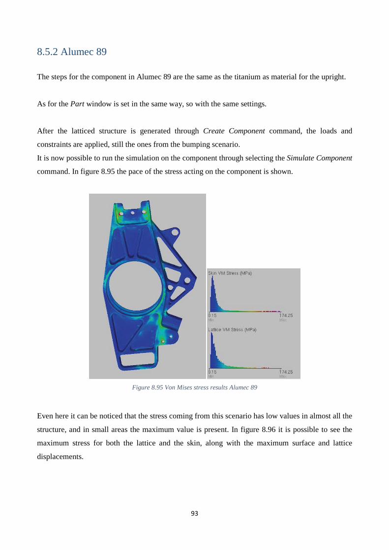
8.5.2 Alumec 89

The steps for the component in Alumec 89 are the same as the titanium as material for the upright.

As for the Part window is set in the same way, so with the same settings.

After the latticed structure is generated through Create Component command, the loads and

constraints are applied, still the ones from the bumping scenario.

It is now possible to run the simulation on the component through selecting the Simulate Component

command. In figure 8.95 the pace of the stress acting on the component is shown.

Figure 8.95 Von Mises stress results Alumec 89

Even here it can be noticed that the stress coming from this scenario has low values in almost all the

structure, and in small areas the maximum value is present. In figure 8.96 it is possible to see the

maximum stress for both the lattice and the skin, along with the maximum surface and lattice

displacements.

93

Figure 8.96 Simulation results Alumec 89, Within 2016

These values are acceptable.

According to the settings imposed, no optimization is required for this component, as that design can

satisfy the load requirements.

Figure 8.97 No optimization required for Alumec 89, Within 2016

The volume reduction coefficient for this model is 0.508.

8.5.3 Steel AISI 4142

The steps for the component in steel AISI 4142 are the same as titanium and aluminium as material

for the upright.

As for the Part window is set in the same way, so with the same settings.

After the latticed structure is generated through Create Component command, the loads and

constraints are applied, still the ones from the bumping scenario.

It is now possible to run the simulation on the component through selecting the Simulate Component

command. In figure 8.98 the pace of the stress acting on the component is shown.

94

Figure 8.98 Von Mises stress results steel AISI 4142

It can be noticed that the stress coming from this scenario has low values in almost all the structure,

and in small areas the maximum value is present. In figure 8.99 it is possible to see the maximum

stress for both the lattice and the skin, along with the maximum surface and lattice displacements.

Figure 8.99 Simulation results steel AISI 4142, Within 2016

These values are acceptable.

According to the settings imposed, no optimization is required for this component using steel, as that

design can satisfy the load requirements.

The volume reduction coefficient for this model is 0.508.

95

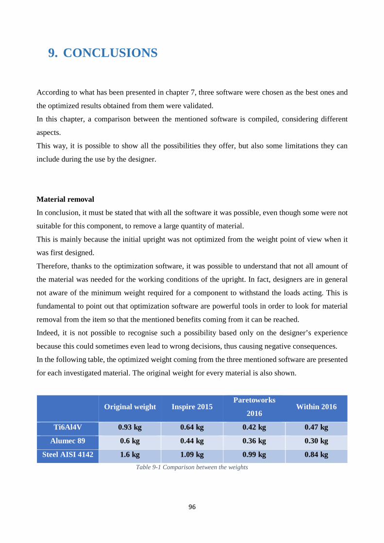
9. CONCLUSIONS

According to what has been presented in chapter 7, three software were chosen as the best ones and

the optimized results obtained from them were validated.

In this chapter, a comparison between the mentioned software is compiled, considering different

aspects.

This way, it is possible to show all the possibilities they offer, but also some limitations they can

include during the use by the designer.

Material removal

In conclusion, it must be stated that with all the software it was possible, even though some were not

suitable for this component, to remove a large quantity of material.

This is mainly because the initial upright was not optimized from the weight point of view when it

was first designed.

Therefore, thanks to the optimization software, it was possible to understand that not all amount of

the material was needed for the working conditions of the upright. In fact, designers are in general

not aware of the minimum weight required for a component to withstand the loads acting. This is

fundamental to point out that optimization software are powerful tools in order to look for material

removal from the item so that the mentioned benefits coming from it can be reached.

Indeed, it is not possible to recognise such a possibility based only on the designer’s experience

because this could sometimes even lead to wrong decisions, thus causing negative consequences.

In the following table, the optimized weight coming from the three mentioned software are presented

for each investigated material. The original weight for every material is also shown.

Original weight Inspire 2015 Paretoworks

2016 Within 2016

Ti6Al4V 0.93 kg 0.64 kg 0.42 kg 0.47 kg

Alumec 89 0.6 kg 0.44 kg 0.36 kg 0.30 kg

Steel AISI 4142 1.6 kg 1.09 kg 0.99 kg 0.84 kg Table 9-1 Comparison between the weights

96

Different shapes

The comparison between the software must be also done based on the different shapes obtained

through the simulation processes.

In fact, since each software uses a specific optimization method, the removal of material is

accomplished in a particular way. The methods, as mentioned in chapter 8, are: SIMP method for

solidThinking Inspire 2015, level-set method for Paretoworks 2016 and SMS method for Autodesk

Within 2016.

This is why, from the figures shown in chapter 8, it is possible to see several results, which can be all

be feasible and fine for the manufacturing of the component. Here the optimized shapes are placed

side by side in order to better show the results coming from each software.

Figure 9.1 - Comparison between the final shapes (Inspire, Paretoworks and Within, from left to right)

It can be noticed that while Inspire removes material by creating big struts connecting the non-design

space, Paretoworks works so that holes are created which extend towards the retained surfaces of the

component under simulation. On the other hand Within removes material from the inside of the item

thus producing small struts connecting the skin.

97

Stress/displacement

According to the stress and displacement values obtained from the simulations, it is possible to

conclude that all the optimized shaped have been validated.

In fact, the values for the Von Mises stress are always below the value of the yield strength for all the

materials in all the optimization software.

The same occurred for the displacement values, which were always below the imposed limit

corresponding to 0.5 mm.

A problem could be noticed within solidThinking Inspire 2015, where some numerical errors were

discovered. However, since they were concluded as numerical errors, even the results coming from

this software are valid.

Limitations

Two of the three software presented some limitations faced during the definition of the settings for

the optimization simulations.

Paretoworks 2016 and Within 2016 had the problem in the definition of the loads and constraints.

As for the constraints, Paretoworks does not give the possibility to constrain a surface in two

directions but only in either one or all of them. Moreover, rotation cannot be locked.

As for the load issue, both Paretoworks and Within had obstacles. The latter gives only the possibility

to apply forces or pressure, that is why it was not possible to apply the braking and cornering scenario:

there is lack of moments among the loads within the boundary condition options. Paretoworks,

instead, gives the possibility to apply moments, but only the axis of rotation of the surface where the

moment itself acts can be defined as the direction of the moment. This is why the moment due to the

cornering could not be applied.

Moreover, Autodesk Within 2016 would also imply a further consideration on the optimized

component, since it creates a lattice structure within the item to optimize. In fact, there should be the

possibility to remove the unused powder in the process to print the component, which in any case is

helpful to support the surfaces during the build. And this can only be accomplished through a post

processing software by creating holes on the skin of the optimized result, as the output file of any

optimized component is in .stl format, which is not possible to handle in a CAD software. In addition,

it could have been interesting if such an analysis had been allowed by the software itself.

Hence, these software present some limitations which restrict hitherto the possibility to widely exploit

them for optimizing components.

98

Cost analysis

As previously mentioned, the costs of the materials needed for producing the upright with the three

materials and according to the best software have been calculated.

It is important to compare the total amount of money needed to produce the optimized component

with powder bed fusion (PBF) methods, the ones used for 3D printing with metals.

They are shown in table 8.1.

Inspire 2015 Paretoworks 2016 Within 2016

Ti6Al4V 128 $ 96 $ 94 $ Alumec 89 26.4 $ 21.6 $ 18 $

Steel AISI 4142 13.1 $ 11.9 $ 10.1 $ Table 9-2 - Production costs

It can be noticed that titanium would imply the most expensive components, due to the highest price

per kg of the powder. This is because the optimized component can actually withstand the loads even

by using another material, that is either aluminium or steel, so similar percentage of material removal

were reached also with the other alloys.

Another important result is about the similar cost deriving from considering Alumec 89 and steel

AISI 4142. This comes from the more percentage of material which was possible to remove with steel

as material for the upright, however the higher density of the steel alloy compared to the aluminium

one brought to this result.

That is why, in order to exploit all the previously mentioned benefits, it would be more convenient to

choose aluminium as the material to keep on producing the upright, even with optimization.

As for the choice of the best software, it seems that until now solidThinking Inspire 2015 (with the

coming updates) is the most complete one in order to cover all the steps from the concept of the

component’s design to its production. This is not only because it provides a result which only need a

smooth operation before the printing, but also because the other software are not capable right now

to provide freedom in the analysis of the component.

99

APPENDIX

Post-processing for braking and cornering analysis with Paretoworks

In order to run an analysis based on the braking and cornering scenario on the optimized upright by

Paretoworks 2016, a manual post-processing was accomplished.

The software used in order to do so is Solid Edge ST7, and the process was time consuming. After

trying to get a shape similar to the one got from the optimization software, the result is shown in

figure A.1 and A.2. The model is one, therefore it contains errors between 6 and 8% of final weight

according to the different material taken into account.

Figure A.1 - Manually optimized component, detail 1 Figure A.2 - Manually optimized component, detail 2

An analysis was run then on the component, applying the loads related with the braking and cornering

scenario. The software used for accomplishing the task was Inspire 2015. The different material were

tested. The results are shown in figures A.3, A.4, A.5, A.6, A.7, A.8 and A.9.

100

Figure A.3 - displacement result, titanium alloy

Figure A.4 - percent of yield result, titanium alloy

101

Figure A.5 - displacement result, aluminium alloy

Figure A.6 - percent of yield result, aluminium alloy

102

Figure A.7 - displacement result, steel alloy

Figure A.8 - percent of yield result, steel alloy

103

Figure A.9 - Von Mises stress results

It can be noticed that even the analysis with this loading scenario brings feasible results, even though

there is no perfect similarity with the component coming from Paretoworks.

Hence, these results can be taken into account for the result considerations.

104

ANSYS Mechanical 14.0 – more results

In this paragraph other results coming from the use of ANSYS Mechanical 14.0 will be presented. For

this case a fine mesh with default element size was used.

By looking at the following pictures, it can be noticed that a finer mesh is even worse than a coarse

one.

Figure A.10 - Overview with fine mesh

Figure A.11 - Fine mesh, detail 1 Figure A.12 - Fine mesh, detail 2

105

Siemens NX 8.5 – more results

In this paragraph other results coming from the use of Siemens NX 8.5 will be presented. For this case

a mesh with element size of 2 mm was used.

The results are shown in the following figures.

It is possible to see how disconnections are still visible.

Figure A.13 - Overview with 2 mm mesh, simulation 1

Figure A.14 - 2 mm mesh, detail 1, simulation 1 Figure A.15 - 2 mm mesh, detail 2, simulation 1

106

Figure A.16 - Overview with 2 mm mesh, simulation 2

Figure A.17 - 2 mm mesh, detail 1, simulation 2 Figure A.18 - 2 mm mesh, detail 2, simulation 2

107

REFERENCES

[1] L. Krog, A. Tucker, G. Rollema, 2002. Application of topology, sizing and shape optimization methods to optimal design of aircraft components. [2] I. Gibson, D. Rosen, B. Stucker, 2015. Additive Manufacturing Technologies, 2nd Edition, Springer. [3] G. I. N. Rozvany, 2007. A critical review of established methods of structural topology optimization. [4] K. Liu, A. Tovar, 2014. An efficient 3D topology optimization code written in Matlab [5] https://arch5541.wordpress.com/2012/11/30/soft-kill-option/ [6] R. Cazacu, L. Grama, 2014. Overview of structural topology optimization medthods for plane and solid structures. [7]A. Krishnakumar, K. Suresh, Hinge-Free Compliant Mechanism Design via the Topological Level-Set [8] K. James, 2012. Aerostructural Shape and Topology Optimization of Aircraft Wings [9] G. Chahine, P. Smith, R. Kovacevic, 2010. Application of Topology Optimization in Modern Additive Manufacturing [10] M. Zhou, R. Fleury, Y.K. Shyy, H. Thomas, J.M. Brennan, 2002. Progress in topology optimization with manufacturing constraints. [11] D. Detwiler, E. Nutwell, D. Lokesha, 2015. Multistage optimization of automotive control arm through topology and shape optimization. [12] W. Saleem, F. Yuqing, W. Yunqiao, 2008. Application of Topology Optimization and Manufacturing Simulations - A new trend in design of Aircraft components [13] N. Snoxall, 2013. Titanium challenge – design proposal. [14] P. B. Prajwal, 2012. Design optimization of Formula One Student sports car upright using Hypermesh. [15] T. Allen, 2010. Suspension Uprights. [16] E. D. Flickinger, 2014. Design and analysis of formula sae car suspension members. [17] Difference Between Aluminum and Titanium. http://www.differencebetween.net/object/difference-between-aluminum-and-titanium/.

108

[18] Titanium and Aluminium. http://www.tilite.com/chairs_titanium-aluminum.php [19] Altair Engineering, Inc. Combining topology optimization with laser additive manufacturing reveals new potential for lightweight structures [20] Arcam EBM system. Ti6Al4V Titanium Alloy [20] W. E. Frazier, 2014. Metal Additive Manufacturing: A Review [21] Alumec 89, 2011. http://www.uddeholm.com/files/PB_alumec_english.pdf [22] Transforming titanium into a low-cost material with 3D printing. http://www.tctmagazine.com/3D-printing-news/transforming-titanium-into-a-low-cost-material-with-3d-print/ [23] Turning additive manufacturing into business. https://www.pwc.nl/en/assets/documents/pwc-turning-additive-manufacturing-into-business.pdf [24] Environmental Impact of Metal Additive Manufacturing. http://www.farinia.com/additive-manufacturing/3d-technique/environmental-impact-metal-additive-manufacturing [25] M. Burkhart, J. C. Aurich, 2015. Framework to predict the environmental impact of additive manufacturing in the life cycle of a commercial vehicle. [26] J. Faludi, C. Bayley, S. Boghal, M. Iribarne, 2014. Comparing Environmental Impacts of Additive Manufacturing vs. Traditional Machining via Life-Cycle Assessment. [27] http://www.enginsoft.it/software/ansys/ [28] http://www.solidthinking.com/productoverview.aspx?item=inspire%20overview&category=products [29] S. Airoldi, 2014. Use of topology optimization techniques in design process (in Italian). [30] http://www.engineering.com/DesignSoftware/DesignSoftwareArticles/ArticleID/10690/Free-SOLIDWORKS-Plug-in-for-Topology-Optimization.aspx [31] http://www.autodesk.com/products/within/overview

109

LIST OF FIGURES REFERENCES

Figure 3.1 – I. Gibson, D. Rosen, B. Stucker, 2015. Additive Manufacturing Technologies, 2nd Edition, Springer.

Figure 3.2 – I. Gibson, D. Rosen, B. Stucker, 2015. Additive Manufacturing Technologies, 2nd Edition, Springer.

Figure 3.3 – R. Cazacu, L. Grama, 2014. Overview of structural topology optimization medthods for plane and solid structures. Figure 3.4 – R. Cazacu, L. Grama, 2014. Overview of structural topology optimization medthods for plane and solid structures. Figure 3.5 – R. Cazacu, L. Grama, 2014. Overview of structural topology optimization medthods for plane and solid structures. Figure 3.6 – A. Krishnakumar, K. Suresh, Hinge-Free Compliant Mechanism Design via the Topological Level-Set Figure 3.7 – A. Krishnakumar, K. Suresh, Hinge-Free Compliant Mechanism Design via the Topological Level-Set Figure 3.8 – R. Cazacu, L. Grama, 2014. Overview of structural topology optimization medthods for plane and solid structures. Figure 3.9 – K. James, 2012. Aerostructural Shape and Topology Optimization of Aircraft Wings Figure 4.4 – E. D. Flickinger, 2014. Design and analysis of formula sae car suspension members. Figure 6.1 – W. E. Frazier, 2014. Metal Additive Manufacturing: A Review Figure 7.1 – Environmental Impact of Metal Additive Manufacturing. http://www.farinia.com/additive-manufacturing/3d-technique/environmental-impact-metal-additive-manufacturing

110