Evaluation of competing software reliability predictions

950 IEEE TRANSACTIONS ON SOFTWARE ENGINEERING, VOL. SE-12, NO.9, SEPTEMBER 1986

Evaluation of Competing Software ReliabilityPredictions

ABDALLA A. ABDEL-GHALY, P. Y. CHAN, AND BEV LITTLEWOOD

Abstract-Different software reliability models can produce very different answers when called upon to predict future reliability in a reliability growth context. Users need to know which, if any, of the competing predictions are trustworthy. Some techniques are presentedwhich form the basis of a partial solution to this problem. Rather thanattempting to decide which model is generally best, the approachadopted here allows a user to decide upon the most appropriate modelfor each application.

Index Terms-Prediction analysis, prediction biasedness and noise,prediction systems, predictive quality, prequential likelihood, software reliability models.

I. INTRODUCTION

SOFTWARE reliability models first appeared in the literature almost 15 years ago [1]-[4], and according to

a recent survey some 40 now exist [5]. There was an initial feeling that a process of refinement would eventuallyproduce definitive models which could be unrese~edly

recommended to potential users. Unfortunately this hasnot happened. Recent studies suggest that the accuracy ofthe models is very variable [6], and that no single modelcan be trusted to perform well in all contexts. More importantly, it does not seem possible to analyze the particular context in which reliability measurement is to takeplace so as to decide a priori which model is likely to betrustworthy.

Faced with these problems, our own research has recently turned to the provision of tools to assist the user ofsoftware reliability models. The basic device we use is ananalysis of the predictive quality of a model. If a userknows that past predictions emanating from a model havebeen in close accord with actual behavior for a particulardata set then he/she might have confidence in future predictions for the same data.

We shall describe several ways of analyzing predictivequality, generally of a fairly informal nature. These techniques will be illustrated using several models to analyzeseveral data sets. Our intention, however, is not to act asadvocates for particular models, although some models doseem to perform noticeably more badly than others.

Manuscript received March 29, 1985; revised August 18, 1985. P. Y.Chan was supported by ICL plc through a research fellowship at the Centrefor Software Reliability, City University. B. Littlewood was supported inpart by the National Aeronautics and Space Administration, and in part byICL plc,

The authors are with the Centre for Software Reliability, City University, Northampton Square, London ECIV OHB, England.

IEEE Log Number 8609734.

Rather, we hope to provide the beginnings of a frameworkwhich will allow a user to have confidence in reliabilitypredictions calculated on an everyday basis.

An important by-product of our ability to analyze predictive quality will be methods of improving the accuracyof predictions. Recent work, to be reported at a later stage,demonstrates some remarkably effective techniques forobtaining better predictions than those coming from"raw" models, and suggests ways in which other "meta"predictors might be constructed.

II. THE SOFTWARE RELIABILITY GROWTH PROBLEMThe theme of this paper is prediction: how to predict

and how to know that predictions are trustworthy.We shall restrict ourselves, for convenience, to the con

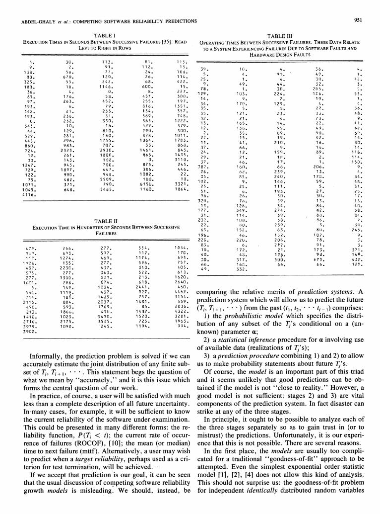
tinuous time reliability growth problem. Tables I, II, andIII show typical data of this kind. In each case the timesbetween successive failures are recorded. Growth in reliability occurs as a result of attempts to fix faults, whichare revealed by their manifestation as failures. A detailedconceptual model of this stochastic process, together withan analysis of the nature of the unpredictability, can befound elsewhere [7], [8].

Different models differ considerably in the ways theyembody these conceptual assumptions in detailed mathematical structure, but the basic problem can be summarized briefly as follows. The raw data available to the userwill be a sequence of execution times t1, t2 , • • • ti - 1 between successive failures. These observed times can beregarded as realizations of random variables T}, T2 , • • •

T,- }. The objective is to use the data, observations on thepast, to predict the future unobserved Ti , · T,+ l e • • • • It isimportant to notice that even the simplest problem concerning measurement of current reliability is a prediction:it involves the future via the unobserved random variablet;

It is this characterization of the problem as a predictionproblem which will underlie all our work reported in thispaper. We contend that the only important issue for a useris whether future behavior can be accurately predicted.Other metrics, such as estimates of the number of faultsleft in a program, are of interest only inasmuch as theycontribute to this overall aim of predicting .with accuracy.Indeed, a recent study [9] of several large IBM systemssuggests that this particular metric can be very misleading: systems with very many faults can have acceptablyhigh reliability if each fault occurs very infrequently.

0098-5589/86/0900-0950$01.00 © 1986 IEEE

ABDEL-GHALY et al.: COMPETING SOFTWARE RELIABILITY PREDICTIONS

TABLE IEXECUTION TIMES IN SECONDS BETWEEN SUCCESSIVE FAILURES [35], READ

LEFT TO RIGHT IN Rows

951

TABLE IIIOPERATING TIMES BETWEEN SUCCESSIVE FAILURES. THESE DATA RELATE

TO A SYSTEM EXPERIENCING FAILURES DUE TO SOFTWARE FAULTS AND

HARDWARE DESIGN FAULTS

3. 30. 113. 81. i 15.9. 2. 91. 1 12. 15.

158. 5u. 77. 24. 10d.33. 67U. 120. 26. 114.

325. 55. 242. 68. 422.180. 10. 1146. 600. 15.

36. 4. o. ~. 227.65. 176. 58. 457. 30n.97. 263. 452. 255. 197.

193. 6. 79. 316. 1351 •143. 21 • 253. 134. 357.193. 256. 31 • 369. 748.

o. 252. 3 .~O. 365. 1222.543. 10. 16. 52? 379.

44. 129. 810. 29U. 3UO.529. 281 • 160. 828. 1011.445. 296. 1 755. 1064. 1 nL3.860. 983. 707. 33. 86d.724. 2323. 2930. 1461. 843.

12. 261. 1800. 865. 1435.30. 143. 108. o. 3110.

1247. 943. 700. 875. 245.729. 1897. 447. 386. 446.122. 990. 948. 1082. 22.

75. 482. 5509. 100. 10.1071 • 371 • 790. 6150. 3321.1045. 648. 5435. 1160. 1864.4116.

TABLE IIEXECUTION TIME IN HUNDRETHS OF SECONDS BETWEEN SUCCESSIVE

FAILURES

479. 266. 277. 554. 1 D.3 4.74'J. 693. 597. 117. 170..... ..., 1274 • 469. 1174. 6 ~ 3.t.: •

1 ()C8. 135 ~ 277. 596. 757.I.3? • 2230. 437. 340. 405.5""5. 277. 363. 522. 613.277. 1300. S Z1. 213. 1620.

1 (,01. 298. 874. 618. 2640.5. '49. 1034. 2441 • 460.

5 'J 5 • 1119. 437. 927. 4462.714. 1~1. 1435. 757. 3154 •

21 15. 884. 2037. 1481 • 559.490. 593. 1769. 85. 2836.213. 1866. 490. 1437. 4322.

1410. 1023. 5470. 1520. 3281 •2716. 2175. 35 'J5. 725. 1963.3979. 1090. '245. 1194. 994.3902.

Informally, the prediction problem is solved if we canaccurately estimate the joint distribution of any finite subset of T;, 1'; + I, · · • . This statement begs the question ofwhat we mean by "accurately," and it is this issue whichforms the central question of our work.

In practice, of course, a user will be satisfied with muchless than a complete description of all future uncertainty.In-many cases, for example, it will be sufficient to knowthe current reliability of the software under examination.This could be presented in many different forms: the reliability function, P(T; < r); the current rate of occurrence of failures (ROCOF), [10]; the mean (or median)time to next failure (mttf). Alternatively, a user may wishto predict when a target reliability, perhaps used as a criterion for test termination, will be achieved. '.

If we accept that prediction is our goal, it can be seenthat the usual discussion of competing software reliabilitygrowth models is misleading: We' should, instead, be

39. 10. I•• ~6. 4.5. 4 • ?1. 49. 1.

25. 1. I•• 30. 4'2.9. 49. 44. 32. 3.

78. 1. 30. 205. rJ.

129. 103. 224. 1f,6. 53.14. 9. 7. 10. 1.3l•• 170. 12? 4 • '1.3). 5 • c' 2 '2. "!,6.J.

35. 121 • 23. 7' lo8.JJ.

~2. 21 • I,. ? s, 9.13. 105. 1 /•• ?2. z i ,

1? • 13(",• 9~) • 49. G?"} 35. 89. 90. {)UL.

22. 15. 19. 42. 14.11. 41 • 210. 16. 30.37. 66. 9. 1b. 1f••2/•• 12. 15 Q • 89. 11&.29. 21 • 1g. 2. 114.37. 46. 17. 1. 150.

38? 16(1. 66. 2CJ6. 9.26. 61.. 239. 13. fl.

05. R5. 240. 17J. 34.102. 9. 146. 59. 4PJ.

25. 25. 111. 5. 31 •51 • (). 193. 27. ~ roJ.

96. 26. 30. 31). 1/.32(1. 70. 39. 13. 13.19. 128. 34. 84. t.().

177. 349. 274. ~2. ~e.

31. 114. 3? 8 ~~ • 3(, •''7' ius. 38. 86. 7.L.)L.

22. »u, 23? 3. Sl,.' •6::;. 1 5? 63. 80. ?,.~.

196. 46. 152. 107. ~.

22S. 220. 20[.. 78. 7.'.33. 6. 21' 2. 91. 3.1(). 172. 21 • 173. 371 •40. 43. 1 2~. 90. 149.30. 317. 5UO. 673. 432.6(,. 16n. 6ft. 66. 120.4() • 332.

comparing the relative merits of prediction systems. Aprediction system which will allow us to predict the future(1';, 1'; + 1, · · · ) from the past (t1, t2, • • • ti - 1) comprises:

1) the probabilistic model which specifies the distribution of any subset of the 1j's conditional on a (unknown) parameter a;

2) a statistical inference procedure for a involving useof available data (realizations of 1j's);

3) a prediction procedure combining 1) and 2) to allowus to make probability statements about future 1j's.

Of course, the model is an important part of this triadand it seems unlikely that good predictions can be obtained if the model is not "close to reality. " However, agood model is not sufficient: stages 2) and 3) are vitalcomponents of the prediction system. In fact disaster canstrike at any of the three stages.

In principle, it ought to be possible to analyze each ofthe three stages separately so as to gain trust in (or tomistrust) the predictions. Unfortunately, it is our experience that this is not possible. There are several reasons.

In the first place, the models are usually too complicated for a traditional "goodness-of-fit" approach to beattempted. Even the simplest exponential order statisticmodel [11, [2], [4] does not allow this kind of analysis.This should not surprise us: the goodness-of-fit problemfor independent identically distributed random variables

952 IEEE TRANSACTIONS ON SOFTWARE ENGINEERING, YOLo SE-IZ, NO.9, SEPTEMBER 1986

ever, that now is an appropriate time to devote less effortto the proliferation of models and more to studies of thiskind.

III. SOME SOFTWARE RELIABILITY GROWTH MODELS

In this section we shall describe briefly some softwarereliability prediction systems. The models described hereare only a small subset of those which appear in the literature (see [5] for a good survey) and so we make noclaims to exhaustiveness.

A. Jelinski and Moranda (JM)

This model [1] is justifiably credited with being the firstreliability growth model specifically created for software.The model due to Shooman [2] appears to be identical toJM and apparently arises from independent work at approximately the same time. The Musa model [4] introduces extra refinements, and has been fairly widely used,but its foundations are essentially identical to JM.

The JM model assumes that T1, Tz, • • • are independent random variables with exponential probability density functions

p(tiIA i) = Aje-A;t; ti > 0 (1)

(3)

(2)

Xi> O.

Ai = (N - i + 1)<1>.

where

The rationale for the model is as follows. When ourobservation of the reliability growth (debugging) begins,the program contains N fa u :ts. Removal of a fault occurswhenever a failure occurs, and at each such event the rateof occurrence of failures is reduced by an amount ¢. Thus¢ can be taken to represent the size of a" fault.

Another way to consider the model is via competingrisks. All faults in a program can be considered to bewaiting for discovery. Their discoveries will occur attimes XI, Xz, · • • XN (for some arbitrary labeling of thefaults) measured from the beginning of debugging. It isassumed that all faults are similar, so that Xi can be treatedas identically distributed. It is further assumed that the Xiare independent and that the common distribution is

The observed stochastic process is thus that process consisting of the first, second, third · · · events (fault discoveries). The times of these events are the order' statistics XCI), XCZ), X(3) ' •••• The interevent times are thespacings between the order statistics:

1j=XCi)-XU - l) (4)

for i = 2, 3, · · · with T I = XCl). It is ~asy to show thatthis formulation via order statistics agrees with (1) and(2).

The unknown parameters of the model, N and <1>, areestimated by maximum likelihood. This forms stage 2) ofthe prediction system. Predictions are made (stage 3)) bythe "plug-in" rule: substitution of these ML estimates

is hard in the presence of unknown parameters. The reliability growth context is much worse because of nonstationarity.

Secondly, properties of the estimators of unknown parameters in these models are usually not available. Forexample, several models assume that the software contains only a finite number of faults. There is thus an upperbound on the number of observable 1)'s. This implies that,for example, we cannot even trust the usual asymptotictheory for maximum likelihood (ML) estimators. Theirsmall sample properties are invariably impossibly hard toobtain.

Bayesians will no doubt argue that there is a "correct"way to build a prediction system for a particular model.It involves posterior distributions of the parameters ofstage 2) and Bayesian predictive distributions for 3). Agood account of this approach in the conventional statistical context is contained in the book by Aitchison andDunsmore [11]. While we agree that this is the best wayforward in principle, and will present some Bayesian predict; on systems in a later section, it is impractical for mostof the proposed models. It is interesting that the classicalstatistical literature has tended to neglect the predictionproblem: ' 'statistics" has usually come to mean onlystage 2) of our triad.

Finally, it could be argued that there are models whichare "obviously" better than others because of the greaterplausibility of their underlying assumptions. We find thisa rather dubious proposition. Certainly, the assumptionsof some models seem overly naive and it might be reasonable to discount them. However, this still leaves others which cannot be rejected a priori. It is our belief thatunderstanding of the processes of software engineering isso imperfect that we cannot even choose an appropriatemodel when we have an intimate knowledge of the software under study. At some future time it may be possibleto match a reliability model to a program via the characteristics of that program: for example, complexity metrics. This is not currently the case.

Where does this leave a user, who merely wants to obtain trustworthy reliability metrics for' is current softwareproject? Our view is that there is no a.. ..mative to a directexamination and comparison of the quality of the predictions emanating from different complete prediction systerns. The intention in this paper is to present the beginnings of a set of tools to assist this examination andcomparison. Although we shall show examples of thesetools applied to the predictions from several predictionsystems using real software reliability data, our intentionis not to recommend particular ways ofpredicting. Rather,it is our experience that no prediction system can betrusted to be always superior to others. Our advice tousers, then, is to be eclectic: try many prediction systemsand use the reliability metrics which are the best for thedata under consideration.

We would not claim that the tools described here arecomplete. Indeed, we shall suggest potentially fruitfulareas for future research. We do believe strongly, how-

ABDEL-GHALY et al.: COMPETING SOFTWARE RELIABILITY PREDICTIONS 953

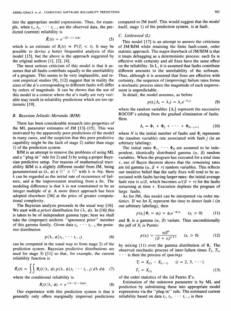
into the appropriate model expressions. Thus, for example, when t b t2, · · · ti _ 1 are the observed data, the predicted (current) reliability is

Ri(t) = e-(N-i+1)~t (5)

which is an estimate of Ri(t) == P(Ti < t). It may bepossible to devise a better frequentist analysis of thismodel [15], but the above is the approach suggested bythe original authors [1], [2], [4].

The most serious criticism of this model is that it assumes that all faults contribute equally to the unreliabilityof a program. This seems to be very implausible, and recent empirical studies [9], [12] suggest that in reality thesizes of the cP' s corresponding to different faults will differby orders of magnitude. It can be shown that the use ofthis model in a context where the cP's really are very variable may result in reliability predictions which are too optimistic [19].

B. Bayesian Jelinski-Moranda (BJM)

There has been considerable research into properties ofthe ML parameter estimates of JM [13]-[15]. This wasmotivated by the apparently poor predictions of the modelin many cases, and the suspicion that this poor predictivecapability might be the fault of stage 2) rather than stage1) of the prediction system.

BJM is an attempt to remove the problems of using MLand a "plug-in' rule for 2) and 3) by using a proper Bayesian predictive setup. For reasons of mathematical tractability BJM is a slightly different model from JM, beingparameterized as (A, cP) E [R1 + X [R1 + with A == N cP. HereA can be regarded as the initial rate of occurrence of failures, and cP the improvement resulting from a fix. Themodeling difference is that A is not constrained to be aninteger multiple of cPo A more direct approach has beenadopted elsewhere [36] at the price of greater computational complexity.

The Bayesian analysis proceeds in the usual way [16].We start with a priori distribution for (A, cP). In [16] thisis taken to be of independent gamma type; here we shalltake the (improper) uniform "ignorance prior" memberof this gamma family. Given data ti , • • • ti _ 1 the posterior distribution

(6)

can be computed in the usual way to form stage 2) of theprediction system. Bayesian predictive distributions areused for stage 3) .[11] so that, for example, the currentreliability function is

i{(t) = 11 Ri(tl A, ~) p O«, ~ It l • • • ti- I ) dA d~ (7)

where the conditional reliability is

Ri(tIA, cP) = e-(A-[i-IJ<!»t. (8)

Our experience with this prediction system is that itgenerally only offers marginally improved predictions

compared to JM itself. This would suggest that the modelitself, stage 1) of the prediction system, is at fault.

c. Littlewood (L)

This model [17] is an attempt to answer the criticismsof JM/BJM while retaining the finite fault-count, orderstatistic approach. The major drawback of JM/BJM is thatit treats debugging as a deterministic process: each fix iseffective with certainty and all fixes have the same effecton the reliability. In L, it is assumed that faults contributedifferent amounts to the unreliability of the software.Thus, although it is assumed that fixes are effective withcertainty, the sequence of (improving) failure rates formsa stochastic process since the magnitude of each improvement is unpredictable.

In detail, the model assumes, as before

p(ti IAi = Ai) = Aie-A;t; (9)

where the random variables {Ai} represent the successiveROCOF's arising from the gradual elimination of faults.Here

Ai = 4>1 + 4>2 + · · · + 4>N-i+ 1 (10)

where N is the initial number of faults and 4>j representsthe (random variable) rate associated with fault j (in anarbitrary labeling).

The initial rates 4>1, • • • 4>N are assumed to be independent, identically distributed gamma (ex, (3) randomvariables. When the program has executed for a total time7, use of Bayes theorem shows that the remaining ratesare iid gamma (ex, (3 + 7) random variables. This reflectsour intuitive belief that the early fixes will tend to be associated with faults having larger rates: the initial averagefault size is exl{3, which becomes exl ({3 + 7) for the faultsremaining at time 7. Execution depletes the program oflarge: faults.

As for JM, this model can be interpreted via order statistics. If we let Xi represent the time to detect fault i (inour arbitrary labeling), then

p(xd 4>i = cPi) = cPie-<!>;X; (Xi> 0) (11)

and 4>i is a gamma (ex, (3) variate. Thus unconditionallythe pdf of Xi is Pareto:

ex{3cx

(i = 2, 3, · · .)

T1 = X(l) (13)

of the order statistics of the iid Pareto X' s.Estimation of the unknown parameter is by ML and

prediction by substituting these into appropriate modelexpressions via the' 'plug-in" rule. The estimated currentreliability based on data t1, t2' · · · t i - 1 is then


where

_ (S + 7 )(&-;+1)&Ri(t) = -",-

{3+7+t(14) Ri(t) = I 1/;(;, S) A T'

Lt + ~ (i, (3)J

where &, pare the ML estimates of the parameters.

(19)

D. Bayesian Littlewood (BL)

This is essentially the same model as in Section III-C,but with a Bayesian predictive analysis. As for BJM,mathematical tractability dictates a reparameterization.Instead of (N, ex, (3) we consider (A, ex, (3) with A == Nee.

A complete Bayesian analysis of this model seems tobe very difficult. Instead, we consider an ad hoc approach. We begin by assuming {3 known, and perform aconventional Bayesian analysis of the unknown (A, ex)using independent gamma priors. The results which aregiven in this paper use the uniform "ignorance prior"versions of these. Predictions are then made in the usualway, but conditional on {3. Finally, an estimator of (3 obtained by a likelihood technique is substituted into thesepredictors.

Details of this work are to appear elsewhere [18].

(21)

(22)

(20)

Prediction is again by ML estimation and the "plugin" rule, so that, for example, the estimated current reliability function after observing t1, t2, · · · ti - 1 is

- -l-SJ~(i'd)Ri(t) - '" .

t + (3

(3l/;(i) At(i) -1 e-{jA;

p(Ai) = r (1/; (i» ·

Here reliability growth, represented by stochasticallydecreasing rates (and thus stochastically increasing T's),occurs when ~ (i) is a decreasing function of i, Again,choice of the parametric form of ~ (i) is under user control. Here we shall use

F. Keiller and Littlewood (KL)

KL [6], [19] is similar to LV, except that reliabilitygrowth is induced via the shape parameter of the gammadistribution for the rates. That is, it makes assumption(14) with

(15)

i-I

7 = ~ t.j= 1 ]

is total elapsed time.

E. Littlewood and Verrall (LV) G. Weibull Order Statistics (W)

(24)

(23)

The JM and L models. can be seen as particular examples of a general class of stochastic processes based onorder statistics. These processes exhibit interevent timeswhich are the spacings between order statistics from arandom sample of N observations with pdf f(x). For JMand L, f(x) is respectively exponential and Pareto. For theW model we assume f(x) is the Weibull density

f(x) == ex{3x(3-ld-a x (3 (x > 0).

H. Duane (D)

The Duane model originated from hardware reliabilitystudies. Duane [21] claimed to have observed in severaldisparate applications that the reliability growth in hardware systems showed the ROCOF having a power lawform in operating time. Crow [22] took this observationand added the assumption that the failure process was anonhomogeneous Poisson process (NHPP) with rate

kbt b-

l (k,b,t> 0).(18)

Estimation from realizations of the T; random variablesis via ML, and prediction via the "plug-in" rule. Details

(17) of this model are to be published elsewhere [18].Other models from this general class of stochastic pro

cess seem attractive candidates for further study [20].

~(i) == ~(i, P) = {31 + f32 i .

This model [3] again treats the successive rates of occurrence of failures, as fixes take place, as random variables. As in JM and BJM, it assumes

p(tiIAi = Ai) = A;e-A; l ; (ti > 0). (16)

The sequence of rates {A;} is treated as a sequence ofindependent stochastically decreasing random variables.This reflects the likelihood, but not certainty, that a fixwill be effective. Detailed reasons for this refinement canbe found in [7], [8]. It is assumed that

[~(i)]aAi -1 e-l/;(i)A;

p(Ai) = T'(«) ,

a gamma distribution with paramet~rs ex, ~ (i).The function ~(i) determines thereliability growth. If,

as is usually the case, ~ (i) is an increasing function of i,it is easy to show that {Ai} forms a stochastically decreasing sequence. Notice how this contrasts with the JM/BJMcase: these fixes are certain (and of equal magnitude). ForLV a fix may make the program less reliable, and even ifan improvement takes place it is of uncertain magnitude.

The choice of parametric family for ~(i) is under thecontrol of the user. In this paper we shall take

Predictions are made by ML estimation of the unknownparameters ex, {3J, (32 and use of the "plug-in" rule. Thusthe estimate of the current reliability function after seeinginterfailure times tJ, t2' · · · ti - 1 is

There is a sense in which an NHPP is inappropriate forsoftware reliability growth. We know that it is the fixeswhich change the reliability, and these occur at a finitenumber of known times. The true rate presumably changes


13635

955

3000

2700

2400

2100 JM

1800

1500

1200

900

LV600

300

decides that he will make his calculations using both JMand LV. Fig. 1 shows the results he would get if he wereusing the data shown in Table I. At each stage, for a particular prediction system, the point plotted is the predicted median of the time to next failure, Ti , based on theavailable data t1, t2' · · · ti - 1. Such plots are thus a simpleway of tracking progress in terms of estimated achievedreliability.

Our user would, we believe, be alarmed at the results.While the models agree that reliability growth is present,they disagree profoundly about the nature and extent ofthat growth. The JM predictions are much more optimistic than those of LV: at any particular stage JM suggeststhat the reliability is greater than LV would suggest.

In addition, the Jlvl'predictions are more "noisy" thanthose of LV. The latter suggests that there is a steady reliability growth with no significant reversals. JM suggeststhat important setbacks are occurring.

What should the user do? He might be tempted to tryyet more prediction systems, and hope to arrive somehowat consensus. If he were to adopt this approach, thechances are that his confusion would increase.

The important point is that he has no guide as to which,if any, of the available predictions is close to the truth. Isthe true reliability as high as suggested by JM in Fig. I?Or are the more conservative estimates of LV nearer to

Fig. 1. Median plots for JM and LV, data from Table I. Plotted are predicted median of T; (based on 1I' 12 , • • • 1;_ I) against i.

(26)

(25)

Again this can be interpreted as the Littlewood modelmixed over a Poisson distributed N variable.

Prediction is via ML estimation and the' 'plug-in" rule.Similar indistinguishability conditions exist between L

and LNHPP as were considered in Section 111-1 [20].

J. Littlewood NHPP (LNHPP)

This model is an NHPP with rate function

The simplest question a user can ask is: how reliable ismy program now? As debugging proceeds, and more interfailure time data are collected, this question is likely tobe repeated. It is hoped that the succession of reliabilityestimates will show a steady improvement due to the removal of faults.

Let us, for the sake of illustration, assume that our useris undemanding, and will be satisfied with an accurate estimate of the median time to next failure at each stage. He

IV. EXAMPLES OF USE

a model first suggested via an ad hoc justification in [37].Presumably such a mixture over a distribution for N

only makes sense to a subjective Bayesian, for which thisdistribution could be taken to represent personal uncertainty about N.

Prediction for this model is, again, via ML estimationand the "plug-in" rule .. Details can be found elsewhere[18] .

Miller, in an interesting recent paper [20], shows thatthis NHPP and the JM model are indistinguishable on thebasis of a single realization of the stochastic process, t1,

t2 , • • • • He notes, however, that inferences for the twowould differ, since they have different likelihood functions. This implies that predictions based on ML inference and the "plug-in" rule would be different.

This is a very curious situation. We have two differentprediction systems, giving different predictions, but basedupon models which are indistinguishable on the basis ofthe data.

discontinuously at these fixes, whereas the NHPP ratechanges continuously. However, recent work [20] suggests that for a single realization it is not possible to distinguish between an order statistic model and an NHPPwith appropriate rate.

Prediction from this model involves ML estimation andthe "plug-in" rule.

I. Goel-Okumoto Model (GO)

It is easy to show [20] that if we treat the parameter Nin the JM model as a Poisson random variable with meanm, the unconditional process is exactly an NHPP with ratefunction


inf i n i ty

>3000

3000

2700

2400

2100

1800

1500

1200

JM dian of T; made 20 steps before (based on t1, • • • ti - 20)

is usually in good agreement with the later "current median" estimate (based on t1, · · · ti - 1)' Even such selfconsistency, though, is no guarantee that these predictions are close to the truth.

It should be pointed out, in fairness, that JM does notalways perform as badly as this: it seems to predict wellfor the data of Table III, for example. However, the performance of JM and all other models varies greatly fromone data set to another. Until recently users had no wayof deciding which, if any, reliability metrics could betrusted. All that was available was a great deal of specialpleading from advocates of particular models: "trust mymodel and you can trust the predictions. " This is not goodenough. No model is totally convincing on a priorigrounds. More importantly, a "good" model is only oneof the three components needed for good predictions.

In the next section we describe some ways in which auser of reliability models can obtain insight into their performance for a particular set ofdata.

900

V . ANALYSIS OF PREDICTIVE QUALITYLV

Fig. 2. Median predictions 20 steps ahead for 1M, LV using data of TableI. 1M makes many excursions to infinity, because it frequently estimatesthe number of remaining faults to be less than 20! The LV predictions20 steps ahead are in close agreement with the (later) 1 step ahead median prediction (shown dotted). This is a useful "self-consistency" property: a prediction system ought to have the property that a predictionfrom Ti based on t I, • • • ti _ 20 is "close" to a later one based on t I, • • •

t, _ I. Clearly 1M does not have this property: compare to Fig. 1. From one of the prediction systems described earlier wecan calculate a predictor

We shall concentrate, for convenience, upon the simplest prediction of all concerning current reliability. Mostof these techniques can be adapted easily to some problems of longer-term prediction, but there are also noveldifficulties arising from these problems. We shall returnto this question later.

Having observed t1, t2, · · · ti- 1 we want to predict therandom variable Ti • More precisely, we want a good estimate of

(28)

(27)Fi(t) == ret, < t)

or, equivalently, of the reliability function

R;(t) = 1 - Fi(t).

............

35

300 J

I

.r.600

reality? Perhaps as important: are the apparent decreasesin reliability indicated by JM real (bad fixes?), or artifactsof the statistical procedures? (The JM model does not, infact, allow for the possibility of bad fixes, so these reversals must be due to stages 2) and 3) of the predictionsystem.)

If our user wished to predict further ahead than the nexttime to failure, he would find the picture even bleaker.Fig. 2 shows how JM and LV perform when required topredict a median 20 steps ahead. That is, prediction ismade of the median of T, at stage i - 20, using observations t1, t2 , • • • t, _20. It is obvious in this case that JM isperforming very badly. Its excursions to infinity arecaused by its tendency to suggest that at stage i - 20 thereare less than 20 faults left in the program, so that the estimated median of T; is infinite. At least LV does not behave in this absurd fashion. In addition it seems reasonably "self-consistent" in that the prediction of the me-

(29)

A user is interested in the "closeness' of Pi (t) to theunknown true F;(t). In fact, interest sometimes centersmerely upon summary statistics such as mean (or median)time to failure, ROCOF, etc. However, the quality ofthese summarized predictions will depend upon the quality of Pi (t), so we shall concentrate on the latter.

Clearly, the difficulty of analyzing the closeness of Pi (t)to F; (t) arises from our never knowing, even at a laterstage, the true F, (t). If this were available (for example,if we simulated the reliability growth data from a sequence of known distributions), it would be possible touse measures of closeness based upon entropy and information [23], or distance measures such as those due toKolmogorov or Cramer-von Mises [24].

In fact, the only information we shall obtain will be asingle realization of the random variable T, when the software next fails. That is, after making the prediction P; (t)


based upon t1, t2, • • • t;- 1, we shall eventually observet., which is a sample of size one from the true distributionF;(t). We must base all our analysis of the quality of predictions upon these pairs {Pi (t), r.}.

Our method will emulate how a user would informallyrespond to a sequence of predictions and outcomes. He/she would inspect the pairs {P;(t), til to see whether thereis any evidence to suggest that the ti ' s are not realizationsof random variables from the Pi (t)' s. If such evidencewere found, it suggests that there are significant differences between Pi (t) and F, (t), i. e., that the predictions arenot in accord with actual behavior. The 20-step ahead predictions of JM shown in Fig. 2 are an example of strongevidence of disagreement between prediction and outcome: the predictions are often of infinite time to failure(program fault-free, so Pi (t) = 0 for all t), but the program always fails in finite time.

Consider the following sequence of transformations:o

957

(30)

Each is a probability integral transform of the observedt, using the previously calculated predictor Pi based upont1, t2 , • • • t,-1' Now, if each Pi were identical to the trueFi , it is easy to see that the u, would be realizations of theindependent uniform U(O, 1) random variables [25], [26].Consequently we can reduce the problem of examiningthe closeness of Pi to F, (for some range of values of i) tothe question of whether the sequence {Ui} "looks like" arandom sample from U(O, 1). Readers interested in themore formal statistical aspects of these issues should consult the recent work of Dawid [26], [27].

Notice that we are not examining the goodness-of-fit ofthe model (stage 1) of the prediction triad. As has beenstated earlier, poor predictions can result from any or allstages of the prediction triad. Specifically, it is possiblefor a "correct" model to be defeated by poor inference.Since technical difficulties often prevent the correct Bayesian analysis of some models, it is particularly importantto examine the fidelity of the predictions themselves. Fortunately, this is an easier technical problem than examining goodness-of-fit of the model alone. In the latter casethe parametric inference is a nuisance, whose influencemust be eliminated in order to detect departures from reality of the model alone. This does not seem to be possibleeven in the case of the simplest order statistic models suchas JM.

We consider now some ways in which the {Ui} sequence can be examined.

A. The u-plot

Since the Ui' s should look like a random sample fromU(O, 1) if the prediction system is working well, the firstthing to examine is whether they appear uniformly distributed. We do this by plotting the sample cumulant distribution function (cdf) of the Ui' S and comparing it to thecdf of U(O, 1), which is the line of unit slope through theorigin. Fig. 3 shows how such a u-plot is drawn. The

Fig. 3. How to draw a u-plot. Each of the n u;'s, with a value between 0and 1, is placed on the horizontal axis. The step function increases byl/(n + 1) at each of these points.

, 'distance" between them can be summarized in variousways. We shall use the Kolmogorov distance, which isthe maximum absolute vertical difference.

In Fig. 4 are shown the u-plots for LV and JM predictions for the data of Table I. The predictions here areF36(t) through FI 35(t) . The Kolmogorov distances are0.190 (JM) and 0.144 (LV). In tables of the Kolmogorovdistribution the JM result is significant at the 1 percentlevel , LV only at the 5 percent level.

From this analysis it appears that neither set of predictions is very good, but that JM is significantly worse thanLV.

In fact the detailed plots tell us more than this. The JMplot is everywhere above the line of unit slope (the U(O,1) cdf); the LV plot almost everywhere below it. Thismeans that the Ui' S from JM tend to be too small and thosefrom LV too large. But u, represents the predicted probability that T, will be less than t., so consistently too smallUi'S suggest that the predictions are underestimating thechance of small t's. That is, the JM plot tells us that thepredictions are too optimistic; the LV plot that these predictions are too pessimistic (although to a less pronounceddegree).

There is evidence from this simple analysis, then, thatthe truth might lie somewhere between the predictionsfrom JM and LV, but somewhat closer to LV. In particular, the true median plot probably lies between the twoplots of Fig. 1. We shall return to this idea in a later section, where further evidence will be given for our beliefthat the two prediction systems bound the truth for thisdata set.

At this stage, then, a user might take an analysis of thiskind to help him make further predictions. He might reasonably adopt a conservative position and decide to useLV for his next prediction, and be reasonably confident


..,.., ,.. -.. "

',.',.":'

JM

, ,. ,

'. ..

.,.' LV

0.5

, , ~ ,Stage 1

ul

u 2 u 3 u 4um-l

u

1m

x. = -en( I - u . )1 1

, ,~ ,Stage 2 -. X

2X 3 X 4

Xm-u

xm

1 i m

normalise Yi = l. xj/I X j1 1

Stage 3 , 1Vv,.0~

Y-;4i ..

Y3~ ~

Fig. 5. Transformations to obtain y-plot.

o 0.5

Fig. 4. LV, JM u-plots, data of Table I. Steps omitted for clarity. Notethat these are reproduced from line-printer plots and do not correspondexactly to true plot.

~ -t- --'O

... .

Fig. 6. JM and LVy-plots for data of Table I. Again, these are line-printerplots and points do not correspond exactly to true points.

C. Measures of "Noise "

It is instructive at this stage to digress a little and consider briefly the estimation problem in classical statistics.

0.5

0.5

...." ,

.:JM" /:'",",,-.

/ #

LV" ~./".

.:1.yo. ~

y-•• i"., ,/.

: .~

" '".' .7., jI'•.~.:·v..

o

This observation is confirmed by a scatter plot of u,against i: Fig. 7. After i = 90 there are only 8 out of 39Ui'S greater than 0.5.

The implication is that the too optimistic predictionsfrom JM are occurring mainly after i = 90. That is, thepoor performance arises chiefly from the later predictions.Since these are based upon larger amounts of data, it isunlikely that stages 2) and 3) of the prediction system areresponsible.

The effect can be seen quite clearly in the median plots(Fig. 1). We can now have reasonable confidence that thesudden increase in the median plot of JM, at about i = 90,is not a true reflection of reliability of the software understudy. It is noticeable that this effect does not occur in theLV predictions.

B. The y-Plot, and Scatter Plot of u 'sThe u-plot treats one type of departure of the predictors

from reality. There are other departures which cannot bedetected by the u-plot. For example, in one of our investigations we found a data set for which a particular prediction system had the property of optimism in the earlypredictions and pessimism in the later predictions. Thesedeviations were averaged out in the u-plot, in which thetemporal ordering of the Ui'S disappears, so that a smallKomogorov distance was observed. It is necessary, then,to examine the Ui'S for trend.

Fig. 5 shows one way in which this can be done. Firstof all, it should be obvious that, since each u, is definedon (0, 1), the sequence u, (Stage 1 in Fig. 5) will looksuper-regular. The transformation Xi = -In (1 - Ui) willproduce a realization of iid unit exponential random variables if the {Ui} sequence really do form a realization ofiid U(O, 1) random variables. That is, Stage 2 of Fig. 5should look like a realization of a homogenous Poissonprocess; the alternative hypothesis (that there is trend inthe Ui'S) will show itself as a nonconstant rate for thisprocess. One simple test is to normalize the Stage 2 process onto (0, 1), as in Stage 3 of Fig. 5, and plot as in theprevious section [28].

Other procedures could be adopted, for example the Laplace test [10], [28], but we think that the plots are moreinformative. For example, see Fig. 6 where this y-plotprocedure is applied to the LV and JM predictions of theTable I data. The Kolmogorov distances are 0.120 (JM)and 0.110 (LV), neither of which are significant at the 10percent level. More interestingly, a close examination ofthe JM y-plot suggests that it is very close to linearity inthe early stages (until about i = 90: see broken line).

that he would not overestimate the reliability of the product.


0.5

1.0

0.0

,,

.Ie

30 50

The median plot of Fig. 1, for example, shows JM tobe more variable than LV. This suggests that the {Fi (t)}sequence for JM is more variable than that for LV. Theimportant question is whether this extra variability of JMis an accurate reflection of what happens to the true{Fi(t) }. Is {Pi (t)} fluctuating rapidly in order to track thetrue {Fi (t)}, or is it exhibiting random sampling fluctuations about a slowly changing {Fi (t)} sequence?

If we had the true {Fi (t)} sequence available, it wouldbe relatively easy to obtain measures akin to variance. Wecould, for example, average the Cramer-von Mises distances between Pi (t) and F,(t) over some range of i. Unfortunately, the {Fi (t)} sequence is not known, and wehave been unsuccessful in our attempts to obtain goodmeasures of the variability between {Pi (t)} and {Fi(t)}.There follow some quite crude measures of variability. InSection V-D we shall consider a global measure whichincorporates both "bias" and "noise": loosely analogous to mse in the classical statistical context.

1) Braun Statistic: Braun [32] has proposed, on obvious intuitive grounds, the statistic

The JM value for the predictions of Table I data is 8.37,for LV 3.18.

For (33), (34), and (35) we can only compare prediction systems on the same data.

where m, is the predicted median of Ti , between differentprediction systems can indicate objectively which is producing the most variable predictions. For example, thegreater variability of the JM medians in Fig. 1 is indicatedby a value of9.57 against LV's 2.96. Of course, this doesnot tell us whether the extra JM variability reflects truevariability of the actual reliability.

3) Rate Variability: A similar comparison can be basedon the ROCOF sequence r, calculated immediately aftera fix:

where B(Ti ) is the estimated mean of If, i.e., the expectation of the predictor distribution, Pi (t), and n is thenumber of terms in the sums. The normalizing denominator is not strictly necessary here, since it will be thesame for all prediction systems and we shall only be comparing values of this statistic for different prediction systems on the same data: there are no obvious ways of carrying out formal tests to see whether a particularrealization of the statistic is "too large. "

2) Median Variability: A comparison of

(34)

(35)

(33)

~ Imi - mi-11l mi-l

L: {ti - E(If)}2i

L: {ti - t}2i

Fig. 7. Scatter plot of u, against i for JM predictions from Table I data.There are "too many" small u's to the right of the dotted line.

There we have a random sample (independent, identicallydistributed random variables) from a population with anunknown parameter, (J. If we assume, for simplicity, that(J is scalar, it is usual to seek an estimator for (J, say 0,which has small mean square error:

mse (0) == E{ (0 - (J)2} (31)

= Var (0) + [bias (0)]2. (32)

There is thus a tradeoff between the variance of the estimator and its bias. It is not obvious, without adoptingextra criteria, how one would choose among estimatorswith the same mse but different variances and biases.

In our prediction problem the situation is much morecomplicated: we wish at each stage to estimate a function,F, (t), not merely a scalar; and the context is nonstationarysince the Fi(t)'s are changing with i. However, the analogy with the classical case has some value. We can thinkof the u-plot as similar to an investigation of bias. Indeed,it is easy to show that, if E{Fi (t)} = F,(t) for all i, theexpected value of the u-plot is the line of unit slope. Thusa systematic deviation between E {Fi (t)} and F, (t) will bedetected by the u-plot.

The fact that we are making a sequence of predictionsin a nonstationary context complicates matters. Thus aprediction system could be biased in one direction forearly predictions and in the other direction for later predictions (and, of course, more complicated deviationsfrom reality are possible). The y-plot is a (crude) attemptto detect such a situation: more sensitive techniques needto be developed.

The u-plot and y-plot procedures then, are an attemptto analyze something analogous to bias. Can we similarlyanalyze "variability" in our more complicated situation?

960 IEEE TRANSACTIONS ON SOFTWARE ENGINEERING, VOL. SE-I2, NO.9, SEPTEMBER 1986

A comparison of two prediction systems, A and B, canbe made via their prequential likelihood ratio

D. Prequential Likelihood

In a series of important recent papers [26], [27], [29],[30], A. P. Dawid has treated theoretical issues concernedwith the validity of forecasting systems. Dawid's discussion of the notion of calibration is relevant to the softwarereliability prediction problem. Here we shall confine ourselves to the prequentiallikelihood (PL) function and, inparticular, the prequential likelihood ratio (PLR). Weshall use PLR as an investigative tool to decide on therelative plausibility of the predictions emanating from twomodels.

The PL is defined as follows. The predictive distribution P; (r) for 1'; based on t1, t2, · · · t. _ 1 will be assumedto have a pdf

Dawid [26] shows that if PLRn ~ 00 as n ~ 00, predictionsystem B is discredited in favor of A.

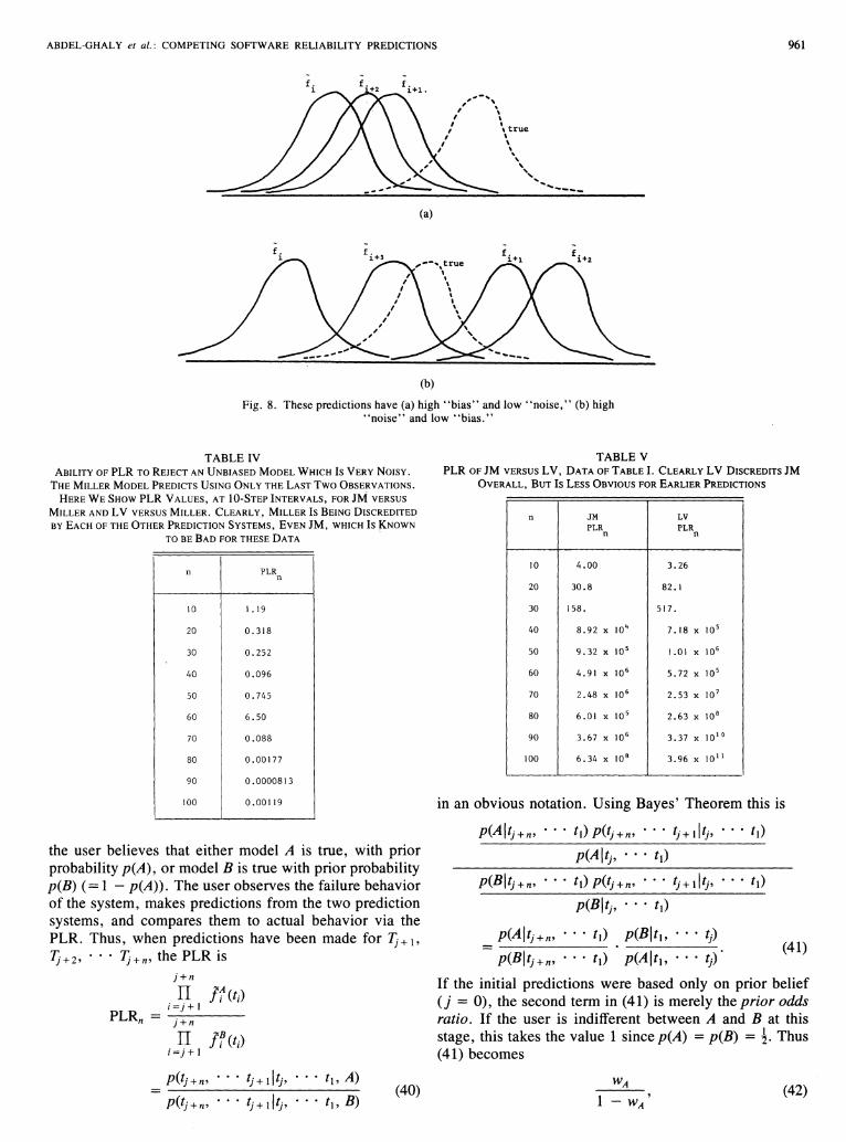
To get an intuitive feel for the behavior of the prequentiallikelihood, consider Fig. 8. Here we consider forsimplicity the problem of predicting a sequence of identically distributed random variables, i.e., F,(t) = F(t),Ii (t) = f(t) for all i. The extension to our nonstationarycase is trivial.

In Fig. 8(a) the sequence of predictor densities are"biased" to the left of the true distribution. Observations, which will tend to fall in the body of the true distribution, will tend to be in the (right hand) tails of thepredictor densities. Thus the prequential likelihood willtend to be small.

In Fig. 8(b) the predictions are very "noisy," but havean expectation close to the true distribution (low' 'bias' ').There is a tendency, again, for the body of the true distribution to correspond to a tail of the predictor (here eitherleft or right tail). Thus the likely observations (from thebody of the true distribution) will have low predictiveprobability density, and the prequential likelihood willtend to be small again.

Notice that this last argument extends to our nonstationary case. Consider the case where the true distributions fluctuate for different values of i, corresponding tooccasional bad fixes, for example. If the predictor sequence were "too smooth," perhaps as a result of

(39)

An extra assumption, that pi(t) was close to Pi-I(t), allowed the latter to be used as an approximate predictor forthe unobserved Ti. Miller's intention was to produce anestimator which had a good u-plot ("unbiased") butwhich was clearly useless. A measure of his success canbe seen by calculating the u-plot and y-plot Kolmogorovdistances for his predictor (based on the previous two observations) on the data of Table I. These are 0.078 and0.069, respectively, which are not significant at the 10percent level. These are much better than LV (0. 14, 0.11)and JM (0.19, 0.12).

Could the prequential likelihood detect the (incorrect)noisiness which renders such a prediction system uselessfor practical purposes? Table IV gives the PLR for JMversus Miller and LV versus Miller. In both cases we thinkit is obvious that the Miller predictions are being discredited.

Of course, this is not a stringent test of the usefulnessof PLR for discriminating between realistic good and badprediction systems. In Table V is shown the PLR of LVagainst JM. There is clear evidence to reject JM in favorof LV. More importantly, there is again strong evidencethat JM is doing particularly badly from about i = 95 (n= 60) onwards. Prior to this, the relative fortunes of thetwo prediction systems fluctuate and it is briefly the casethat JM is preferred.

One interpretation of the PLR, when A and B are Bayesian prediction systems [11], is as an approximation to theposterior odds of model A against model B. Suppose that

smoothing from an inference procedure, this would be detected. The observations would tend to fall in the bodiesof the (noisy) true distributions, and hence in the tails ofthe predictors, giving a small prequentiallikelihood.

Thus the prequential likelihood can in principle detectpredictors which are too noisy (when the true distributionsare not variable) and predictors which are too smooth(when the true distributions are variable). This contrastswith the measures of variability proposed in Section V-C:here we' could detect noise in a predictor, but could nottell whether it reflected actual noise in the reliability.

The prequentiallikelihood, then, should allow us to detect both consistent deviations between prediction andreality ("bias"), and large variability in the distance between prediction and reality (" noise' '). In this sense it isanalogous to mse in parameter estimation (31), (32).

In fact it is possible to construct predictors which are(almost) exactly unbiased, but are useless in practice because of their great noisiness. An example is suggestedby Miller [31]. He proposed, as a counterexample to theefficacy of the u-plot procedure, an estimator based onlyupon the previous one or two observations. His idea wasto assume that the {Ti} sequence were exponential random variables, and estimate the mean of T, _1 by usingti- 1 or by using (ti- 1 + ti- 2)/2. In each case he contrivedto obtain a predictor for T,- 1, Pi- 1(t), which was unbiased:

(38)

(36)

(37)

~ d -J;(t) = dt F;(t).

j+n

PLn = II /;(t;).;=j+I

j+n

II 11 (t;);=j+ 1

PLRn = j+n

II 17(t;);=j+ 1

For such one-step-ahead predictions of 1)+1,1)+2,

1J+n the prequentiallikelihood is


,"'-',, ,, \, \

: "true, \, \I \

",,",

........_---(a)

(b)

Fig. 8. These predictions have (a) high "bias" and low "noise," (b) high"noise" and low "bias."

TABLE V

PLR OF JM VERSUS LV, DATA OF TABLE I. CLEARLY LV DISCREDITS JM

OVERALL, BUT Is LESS OBVIOUS FOR EARLIER PREDICTIONS

in an obvious notation. Using Bayes' Theorem this is

p(AItj +n' • • • t1)p(tj +n' • • • tj + II tj , • • • t1)

p(Altj , • • • t 1)

(41)

n JM LVPLR PLR

n n

10 4.00 3.26

20 30.8 82.1

30 158. 517.

40 8.92 x 10" 7.18 X 105

50 9.32 X 105 1.01 X 106

60 4.91 X 106 5.72 X 105

70 2.48 X 106 2.53 X 107

80 6.01 X 105 2.63 X 108

90 3.67 X 106 3.37 X 101 0

100 6.34 X 108 3.96 X lOll

p(B\tj + n' • • • t1) p(tj + n' • • • tj + t1 tj , • • • tl)

p(Bltj , • • • t 1)

p(Altj +n' t l ) p(Bltb tj )

p(Bltj + n , t1) p(Altb tj ) '

If the initial predictions were based only on prior belief(j = 0), the second term in (41) is merely the prior oddsratio. If the user is indifferent between A and B at thisstage, this takes the value 1 since p(A) = p(B) = ~. Thus(41) becomes

j+n

IT If (t i )i=j+ 1

n PLRn

10 l. 19

20 0.318

30 0.252

40 0.096

50 0.745

60 6.50

70 0.088

80 0.00177

90 0.0000813

100 0.00119

TABLE IV

ABILITY OF PLR TO REJECT AN UNBIASED MODEL WHICH Is VERY NOISY.

THE MILLER MODEL PREDICTS USING ONLY THE LAST Two OBSERVATIONS.

HERE WE SHOW PLR VALUES, AT to-STEP INTERVALS, FOR JM VERSUS

MILLER AND LV VERSUS MILLER. CLEARLY, MILLER Is BEING DISCREDITED

BY EACH OF THE OTHER PREDICTION SYSTEMS, EVEN JM, WHICH Is :J(NOWN

TO BE BAD FOR THESE DATA .

the user believes that either model A is true, with priorprobability p(A) , or model B is true with prior probabilityp(B) (= 1 - p(A)). The user observes the failure behaviorof the system, makes predictions from the two predictionsystems, and compares them to actual behavior via thePLR. Thus, when predictions have been made for 1J+I,1J+2' • • • 1J+n' the PLR is

j+n

IT 11 (t i )i=j+ 1

t), B)(40) (42)


TABLE VI

ANALYSIS OF DATA OF TABLE I USING THE PREDICTION SYSTEMS DESCRIBED

IN THE PAPER. IN THIS, AND THE FOLLOWING TABLES, THE INSTANTANEOUS

MEAN TIME TO FAILURE (IMTTF) Is USED INSTEAD OF THE PREDICTED

MEAN IN THE CALCULATING OF THE BRAUN STATISTIC FOR BJM, BL, D,

GO, LNHPP, W. THIS Is BECAUSE THE MEAN DOES NOT EXIST, OR Is

HARD TO CALCULATE. THE IMTTF Is DEFINED TO BE THE RECIPROCAL OF

THE CURRENT ROCOF. NOTE (1) THAT FOR L THE ML ROUTINE DOES NOT

ALWAYS TERMINATE NORMALLY, SO WE ARE NOT CERTAIN THAT TRUE ML

ESTIMATES ARE BEING USED. IT Is POSSIBLE THAT WE COULD GET BETTER

L PREDICTORS BY ALLOWING THE ML SEARCH ROUTINE TO RUN LONGER

-loge (PL)

(ranks)

y-plotKS distance(sig. level)

u-plotKS distance(s i g , level)

Braunstatistic(rank)(rank)

r . - r . I~ ~-l

(rank)Model

l======:==========i========================;:::=============:;:::=:::========::::::;=::=====

JM 9.57(8)

8.37( 10)

I. 31( 10)

.190( 1%)

.120(NS)

770.3(9)

BJM 7.21(8)

1. II(9)

.170( 1%)

.116(NS)

770.7(10)

6.82(5)

6.23(6)

0.86(3)

.109(NS)

.069(NS)

762.4(2)

BL3. 72

(4)0.83

(2).119(NS)

.075(NS)

763.0(3)

LV2.96

(2)3.18

(2)0.90

(7).144(5%)

.110(NS)

764.9(6)

KL 2.79(1)

3.26(3)

0.88(5)

.138(5%)

.109(NS)

764.7(5)

D3. II

(3)2.92

(1)0.89

(6).159(2%)

.093(NS)

765.3(7)

GO 8.62(7)

7.34(9)

1. I I(8)

.153(2%)

.125( 10%)

768.6(8)

LNHPP4.16

(4)3.84

(5)0.82(I)

.081(NS)

.064(NS)

761.4(1)

w 7.38(6)

6.61(7)

0.86(4)

.075(NS)

.075(NS)

763.0(3)

the posterior odds ratio, with WA representing his posterior belief that A is true after seeing the data (i. e., aftermaking predictions and comparing them with actual outcomes).

Of course, the prediction systems considered in SectionIII are not all Bayesian ones. It is more usual to estimatethe parameters via ML and use the "plug-in" rule forprediction. Dawid, however, shows [26] that this procedure and the Bayesian predictive approach are asymptotically equivalent.

It is, in addition, not usual to allow j = 0 in practice.Although Bayesians can predict via prior belief withoutdata, non-Bayesians usually insist that predictions arebased on actual evidence. In practice, though, the valueof j may be quite small.

With these reservations, we do think that (42) can beused as an intuitive interpretation of PLR. We shall usethis idea, with some caution, in later sections.

VI. EXAMPLES OF PREDICTIVE ANALYSIS

In this section we shall use the devices of the previoussection to analyze the predictive quality of several prediction systems on the three data sets of Tables I, II, and III.We emphasize that our primary intention is not to pick a"universally best" prediction system. Rather, we hope to

show how a fairly informal analysis can help a user toselect, for a particular data source, reliability predictionsin which he/she can have trust. Our own analyses suggestthat one should approach a new data source without preconceptions as to which prediction system is likely to bebest: such preconceptions are likely to be wrong.

Consider first the data of Table I. Table VI summarizesour results concerning the quality of performance of thevarious prediction systems on these data.

In Table VI, it can be seen that LNHPP comes first onthe PL ranks, followed by L, then BL, LV, KL, and W.The Braun statistic rankings closely follow the PL ranks.

Both Land LNHPP have non significant u-plot and yplot distances, although LNHPP has a smaller u-plot distance. This might suggest that LNHPP is slightly betteron the' 'bias" criterion. For noise, each of these prediction systems has similar rankings on the median and ratestatistics, but in each case the value for LNHPP is smallerthan that for L.

In fact, the predictions from Land LNHPP are verysimilar. Fig. 9 shows their median predictions along withthose of JM and LV shown earlier in Fig. 1. Notice thatthese predictions are less pessimistic than LV, less optimistic than JM, but are closer to LV: this adds weight toour analysis of the LV and JM predictions in Section V.


3000

KL

w

136

3000

2700

2400

2100

1800

1500

1200

900

600

300

35

(6 shown dotted)

LNHPP

/ LV,-

13635

II JMIIII

•,.it:, III

I,," I, '/, I II"~ I, I I

\ I ~ I " " ,'I~ ,I '" .'.

{1 .: ',\ ; ~\:

II~: "~

:'" !If\.: fV\ f

600 J : ! { -..'-' '" '", ;' '-",\.. ,\ .." .. -',,"

300 ' '''',' , ,~J--_/-'--

'~/-~~'

900

1200

1500

1800

2100

2400

2700

____"t~, ...~

(a) (b)

Fig. 9. (a) Median predictions from L, NHPP, LV, JM for data of TableI. Land LNHPP are virtually indistinguishable for many predictions.The (dotted) excursions of L could be "spurious," resulting from nonconvergence of the ML optimization algorithm. (b) Median predictionsfrom Wand KL for data of Table I. KL is very close to LV, so latter notplotted.

The slightly worse PL value for L compared to LNHPPis probably accounted for by its extra noise, as shown bythe median plot and the median and rate difference statistics.

Of the high PL-ranking predictions, that leaves BL, KL,and W. Unfortunately, it is not easy to calculate mediansfor BL, so these are not shown in Fig. 9. KL gives resultswhich are very similar to LV: significantly too pessimisticon the u-plot. W is nonsignificant on both u- and y-plotsbut (as for L) is noisier on both the statistics and the plot.Since u- and y-plot distances are so small, this noisinessprobably explains its relatively poor performance on thePL.

If we take the best six prediction systems (L, BL, LV,KL, LNHPP, and W) and discount BL (because we cannot compute the medians), LV and KL (because they exhibit significant "bias" as evidenced by the u-plot) weare left with L, LNHPP, andW, The agreement betweentheir median predictions is striking (see Fig. 9).

What conclusions could a user draw from all this? Weassume that he/she wishes to make predictions' about thefuture and has available the data of Table I upon whichour analysis is based. We also assume that he/she is prepared to trust for future predictions a prediction systemwhose past predictions have been shown to be close toactual observation (roughly this means that the future de-

velopment of the software is similar to the past: there isno discontinuity between past and future). In that case wewould suggest that, for this data source, a user makes afuture prediction using LNHPP.

Notice that it is possible for the "preferred predictionsystem" to change as the data vector gets larger. For example, based on the whole of the Table I data LV is preferable to JM; on the first 60 observations JM is better thanLV (see Table V). Thus, our advice to a user to useLNHPP is strictly only applicable for the next prediction.In principle this analysis should be repeated at each step.In practice this is sometimes not necessary: we have foundthat changes usually take place fairly slowly so that relatively infrequent checks on predictive quality are sufficient. However, these analyses are not computationallyonerous when compared to the numerical optimizationsneeded for the ML estimation at each step.

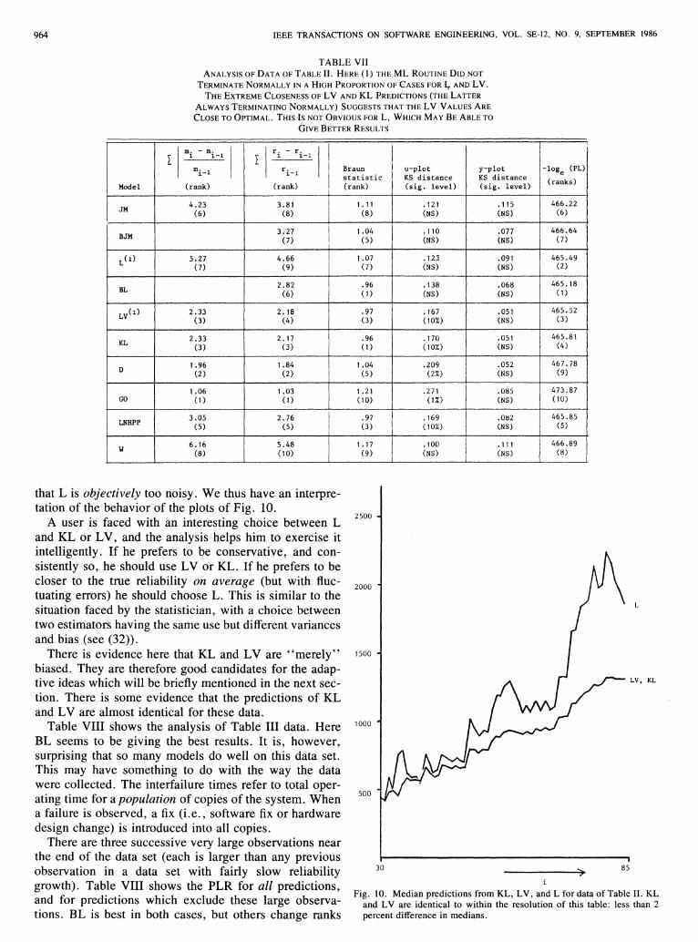
Table VII shows a similar analysis of the data of TableII. The prequential likelihood suggests that L, BL, LV,and KL perform best. A more detailed study shows aninteresting tradeoff between' 'bias" and' 'noise. " The KLand LV u-plot distances are significant and the plots areboth below. the line of unit slope, indicating that the predictions are too pessimistic. The noise statistics based onmedians and rates show that L is more noisy than LV andKL. Since they give similar PL values we can conclude


TABLE VIIANALYSIS OF DATA OFTABLE II. HERE (1) THE ML ROUTINE DID NOT

TERMINATE NORMALLY IN AHIGH PROPORTION OFCASES FOR I, AND LV.THE EXTREME CLOSENESS OFLV AND KL PREDICTIONS (THELATTER

ALWAYS TERMINATING NORMALLY) SUGGESTS THAT THE LV VALUES ARECLOSE TOOPTIMAL. THISIs NOT OBVIOUS FOR L, WHICH MAyBE ABLETO

GIVEBETTER RESULTS

I mi - mi-l I I r. - r. I II L 1 1-1

mi_ 1

r . Braun I u-plot y-plot -loge (PL)1-1

statistic I KS distance KS distanceModel (rank) (rank) (rank) (s i g , level) (s i g , level)

(ranks)

4.23 3.81 1. 11 .121 .115 466.22JM (6) (8) (8) (NS) (NS) (6)

3.27 I 1.04I

.110 .077 466.64BJM (7) (5) (NS) (NS) (7)

L (1) 5.27 4.66 1.07 .123 .091 465.49(7) (9) (7) (NS) (NS) (2)

2.82 .96 .138 .068 465.18BL (6) (1) (NS) (NS) (1)

LV(l) 2.33 2.18 .97 .167 .051 465.52(3) (4) (3) (10%) (NS) (3)

2.33 2.17 .96 .170 .051 465.81KL (3) (3) (1) (10%) (NS) (4)

1.96 1.84 1.04 .209 .052 467.78D (2) (2) (5) (2%) (NS) (9)

1.06 1.03 1.21 .271 .085 473.87GO (1) (1) (10) (1%) (NS) (10)

3.05 2.76 .97 I .169 .082 465.85LNHPP (5) (5) (3) I (10%) (NS) (5)

6.16 5.48 1.17 .100 .111 466.89W (8) (10) (9) (NS) (NS) (8)

that L is objectively too noisy . We thus have an interpretation of the behavior of the plots of Fig. 10.

A user is faced with an interesting choice between Land KL or LV, and the analysis helps him to exercise itintelligently. If he prefers to be conservative, and consistently so, he should use LV or KL. If he prefers to becloser to the true reliability on average (but with fluctuating errors) he should choose L. This is similar to thesituation faced by the statistician, with a choice betweentwo estimators having the same use but different variancesand bias (see (32».

There is evidence here that KL and LV are "merely"biased. They are therefore good candidates for the adaptive ideas which will be briefly mentioned in the next section. There is some evidence that the predictions of KLand LV are almost identical for these data.

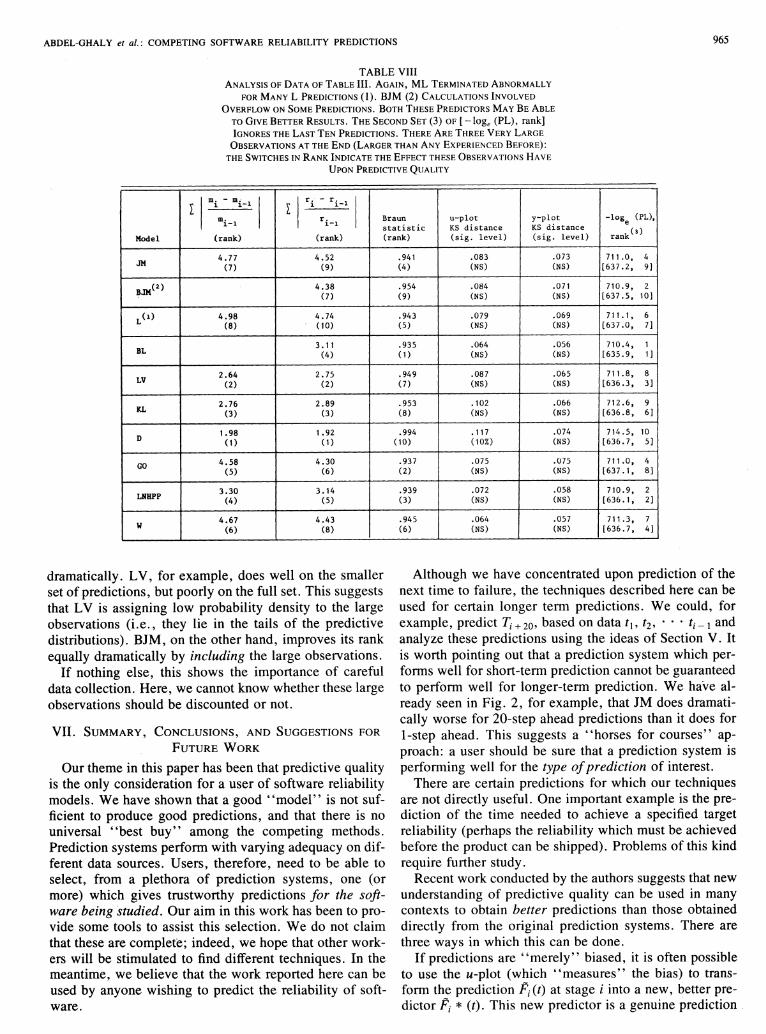
Table VIII shows the analysis of Table III data. HereBL seems to be giving the best results. It is, however,surprising that so many models do well on this data set.This may have something to do with the way the datawere collected. The interfailure times refer to total operating time for a population of copies of the system. Whena failure is observed, a fix (i.e., software fix or hardwaredesign change) is introduced into all copies.

There are three successive very large observations nearthe end of the data set (each is larger than any previousobservation in a data set with fairly slow reliabilitygrowth). Table VIII shows the PLR for all predictions,and for predictions which exclude these large observations. BL is best in both cases, but others change ranks

2500

2000

L

1500

LV, KL

1000

500

Fig. 10. Median predictions from KL, LV, and L for data of Table II. KLand LV are identical to within the resolution of this table: less than 2percent difference in medians.


TABLE VIII

ANALYSIS OF DATA OF TABLE III. AGAIN, ML TERMINATED ABNORMALLY

FOR MANY L PREDICTIONS (1). BJM (2) CALCULATIONS INVOLVED

OVERFLOW ON SOME PREDICTIONS. BOTH THESE PREDICTORS MAyBE ABLE

TO GIVE BETTER RESULTS. THE SECOND SET (3) OF [-loge (PL), rank]IGNORES THE LAST TEN PREDICTIONS. THERE ARE THREE VERY LARGE

OBSERVATIONS AT THE END (LARGER THAN ANY EXPERIENCED BEFORE):

THE SWITCHES IN RANK INDICATE THE EFFECT THESEOBSERVATJONS HAVE

UPON PREDICTIVE QUALITY

L I mim~ mi_l I L I

ri

- ri_1

Ir. Braun u-plot y-plot -loge (PL),1-1 1-1

statistic KS distance KS distanceModel (rank) (rank) (rank) (s i g , level) (s i g , level) rank(3)

JM4.77 4.52 .941 .083 .073 711.0, 4

(7) (9) (4) (NS) (NS) [637.2, 9]

BJM(2) 4.38 .954 .084 .071 710.9, 2(7) (9) (NS) (NS) [637.5, 10]

L(1) 4.98 4.74 .943 .079 .069 711.1, 6(8) (10) (5) (NS) (NS) [637.0, 7]

BL 3.11 .935 .064 .056 710.4, 1(4) (1) (NS) (NS) [635.9, 1]

LV 2.64 2.75 .949 .087 .065 711.8, 8(2) (2) (7) (NS) (NS) [636.3, 3]

KL2.76 2.89 .953 .102 .066 712.6, 9

(3) (3) (8) (NS) (NS) [636.8, 6]

D1.98 1.92 .994 .117 .074 714.5, 10

(1) (1) (10) (10%) (NS) [636.7, 5]

GO 4.58 4.30 .937 .075 .075 711.0, 4(5) (6) (2) (NS) (NS) [637.1, 8]

LNHPP 3.30 3.14 .939 .072 .058 710.9, 2(4) (5) (3) (NS) (NS) [636.1, 2]

W4.67 4.43 .945 .064 .057 711.3, 7

(6) (8) (6) (NS) (NS) [636.7, 4]

965

dramatically . LV, for example, does well on the smallerset of predictions, but poorly on the full set. This suggeststhat LV is assigning low probability density to the largeobservations (Le., they lie in the tails of the predictivedistributions). BJM, on the other hand, improves its rankequally dramatically by including the large observations.

If nothing else, this shows the importance of carefuldata collection. Here, we cannot know whether these largeobservations should be discounted or not.

VII. SUMMARY, CONCLUSIONS, AND SUGGESTIONS FOR

FUTURE WORK

Our theme in this paper has been that predictive qualityis the only consideration for a user of software reliabilitymodels. We have shown that a good "model" is not sufficient to produce good predictions, and that there is nouniversal "best buy" among the competing methods.Prediction systems perform with varying adequacy on different data sources. Users, therefore, need to be able toselect, from a plethora of prediction systems, one (ormore) which gives trustworthy predictions for the software being studied. Our aim in this work has been to provide some tools to assist this selection. We do not claimthat these are complete; indeed, we hope that other workers will be stimulated to find different techniques. In themeantime, we believe that the work reported here can beused by anyone wishing to predict the reliability of software.

Although we have concentrated upon prediction of thenext time to failure, the techniques described here can beused for certain longer term predictions. We could, forexample, predict Ti + 20, based on data t}, t2 , • • • ti - 1 andanalyze these predictions using the ideas of Section V. Itis worth pointing out that a prediction system which performs well for short-term prediction cannot be guaranteedto perform well for longer-term prediction. We have already seen in Fig. 2, for example, that JM does dramatically worse for 20-step ahead predictions than it does forI-step ahead. This suggests a "horses for courses" approach: a user should be sure that a prediction system isperforming well for the type ofprediction of interest.

There are certain predictions for which our techniquesare not directly useful. One important example is the prediction of the time needed to achieve a specified targetreliability (perhaps the reliability which must be achievedbefore the product can be shipped). Problems of this kindrequire further study.

Recent work conducted by the authors suggests that newunderstanding of predictive quality can be used in manycontexts to obtain better predictions than those obtaineddirectly from the original prediction systems. There arethree ways in which this can be done.

If predictions are "merely" biased, it is often possibleto use the u-plot (which "measures" the bias) to transform the prediction Pi (t) at stage i into a new, better predictor Pi * (t). This new predictor is a genuine prediction.

966 IEEE TRANSACTIONS ON SOFTWARE ENGINEERING, YOLo SE-12, NO.9, SEPTEMBER 1986

system since it depends only upon data t l , t2, · • · t i - 1

seen before the random variable T, is predicted. A simpleprocedure to produce systems which "learn from their pastmistakes" in this way is described in [33]. Our recentwork, which improves on these naive adaptive approaches, will be reported at a later time.

We saw earlier in this paper that there are sometimesreversals of relative performance between different prediction systems for a given data set. For the data of TableI, for example, LV is better overall than JM, but JM isslightly superior at an earlier stage. Rather than predictingby using only one or the other prediction system, a Bayesian interpretation of PLR as posterior odds would suggest forming a meta-predictor: a linear combination of thetwo (or more) predictions with the weights chosen in someoptimal way (e.g., posterior probabilities). We have hadsome success with this technique, particularly using narrow windows to quickly detect changes in preference, andwill report our results at length in a later paper.

Apart from "bias," the other major departure fromreality which can be exhibited by a prediction system isunwarranted noisiness. A prediction system which is unbiased but too noisy is a candidate for smoothing. Ofcourse, fairly short-term smoothing will be necessary inthese nonstationary contexts, so as not to introduce bias.

Combinations of all three of these approaches are possible, and will result in a rich family of meta-predictors.In all cases, users do not need to trust the predictions apriori, but can use the techniques of this paper to examinethem objectively.

The central theme of our recent work has been a shiftof emphasis from model to prediction. We do not claimthat these techniques for examining predictive accuracyare exhaustive; indeed, we hope that other workers willfind the problem of sufficient interest to seek new tools.We do, however, feel that the general approach holdsgreat promise, not least in the potentiality for devising"prediction improvement" schemes. Our current research centers on this latter problem, and we expect toreport some encouraging preliminary results in the nearfuture.

ACKNOWLEDGMENT

This work has been helped over the past couple of yearsby the kind provision of data by several individuals. Wehave also benefitted greatly from discussions with manypeople. We would particularly like to single out T. Anderson, P. Dawid, M. Dyer, I. Goudie, N. Harris, E.Migneault, and D. Miller.

Our thanks to G. Palmer, who typed this and corrected(some) of our mistakes.

REFERENCES

[1] Z. Jelinski and P. B. Moranda, "Software reliability research," inStatistical Computer Performance Evaluation, W. Freiberger, Ed.New York: Academic, 1972, pp. 465-484.

[2] M. Shooman, "Operational testing and software reliability during

program development," in Rec. 1973 IEEE Symp. Comput. SoftwareRel., New York, Apr. 30-May 2, 1973, pp. 51-57.

[3] B. Littlewood and J. L. Verrall, "A Bayesian reliability growth modelfor computer software," J. Roy. Statist. Soc. C, vol. 22, pp. 332346, 1973.

[4] J. D. Musa, "A theory of software reliability and its application,"IEEE Trans. Software Eng., vol. SE-l, pp. 312-327, Sept. 1975.

[5] C. J. Dale, "Software reliability evaluation methods," British Aerospace Dynamics Group, Rep. ST-26750, 1982.

[6] P. A. Keiller, B. Littlewood, D. R. Miller, and A. Sofer, "Comparison of software reliability predictions," in Dig. FTCS 13 (l3th Int.Symp. Fault-Tolerant Comput., 1983, pp. 128-134.

[7] B. Littlewood, "How to measure software reliability and how notto," IEEE Trans. Rel., vol. R-28, pp. 103-110, June 1979.

[8] J. C. Laprie, "Dependability evaluation of software systems in operation," IEEE Trans. Software Eng., vol. SE-I0, pp. 701-714, Nov.1984.

[9] E. N. Adams, "Optimizing preventive service of software products,"IBM J. Res. Develop., vol. 28, no. 1, 1984.

[10] H. Ascher and H. Feingold, Repairable Systems Reliability (LectureNotes in Statistics, No.7). New York: Dekker, 1984.

[11] J. Aitchison and 1. R. Dunsmore, Statistical Prediction Analysis.Cambridge: Cambridge University Press, 1975.

[12] P. M. Nagel and J. A. Skrivan, "Software reliability: Repetitive _runexperimentation and modelling," Boeing Comput. Services Company, Seattle, WA, Rep. BCS-40399, Dec. 1981.

[13] E. H. Forman and N. D. Singpurwalla, "An empirical stopping rulefor debugging and testing computer software, " J. Amer. Statist. Ass. ,vol. 72, pp. 750-757, Dec. 1977.

[14] B. Littlewood and J. L. Verrall, "On the likelihood function of adebugging model for computer software reliability," IEEE Trans.Rel., vol. R-30, pp. 145-148, June 1981.

[15] H. Joe and N. Reid, "Estimating the number of faults in a system,"J. Amer. Statist. Ass., vol. 80, pp. 222-226, Mar. 1985.

[16] B. Littlewood and A. Sofer, "A Bayesian modification to the Jelinski-Moranda software reliability growth model," available from firstauthor.

[17] B. Littlewood, "Stochastic reliability growth: A model for fault-removal in computer programs and hardware designs," IEEE Trans.Rel., vol. R-30, pp. 313-320, Oct. 1981.

[18] A. A. Abdel-Ghaly, Ph.D. dissertation, City Univ., London, 1986.[19] P. A. Keiller, B. Littlewood, D. R. Miller, and A. Sofer, "On the

quality of software reliability predictions," in Proc. NATO ASI Electron. Syst. Effectiveness and Life Cycle Costing, Norwich, England.Berlin: Springer, 1983, pp. 441-460.

[20] D. R. Miller, "Exponential order statistic models of software reliability growth," George Washington Univ., Washington, DC, Tech.Rep. T-496/84, 1984.

[21] J. T. Duane, "Learning curve approach to reliability monitoring,"IEEE Trans. Aerosp., vol. AS-2, pp. 563-566, 1964.

[22] L. H. Crow, "Confidence interval procedures for reliability growthanalysis," U.S. Army Material Syst. Anal. Activity, Aberdeen, MD,Tech. Rep. 197, 1977.

[23] H. Akaike, "Prediction and Entropy," Math. Res. Center, Univ.Wisconsin-Madison, MRC Tech. Summary Rep., June 1982.

[24] M. G. Kendall and A. Stuart, The Advanced Theory of Statistics.London: Griffin, 1961.

[25] M. Rosenblatt, "Remarks on a multivariate transformation," Ann.Math. Statist., vol. 23, pp. 470-472, 1952.

[26] A. P. Dawid, "Statistical theory: The prequential approach," J. Roy.Statist. Soc. A, vol. 147, pp. 278-292, 1984.

[27] -, "Calibration-based empirical probability," Dep. Statist. Sci.,University College, London, Res. Rep. 36, 1984.

[28] D. R. Cox and P. A. W. Lewis, Statistical Analysis of Series ofEvents. London: Methuen, 1966.

[29] A. P."Dawid, "The well-calibrated Bayesian" (with discussion), J.Amer. Statist. Ass., vol. 77, pp. 605-613, 1982.

[30] A. P. Dawid, "Probability forecasting," in Encyclopedia of Statistical Sciences, vol. 6, S. Kotz, N. L. Johnson, and C. B. Read, Eds.New York: Wiley-Interscience, to be published.

[31] D. R. Miller, private communication, 1983.[32] H. Braun and J. M. Paine, "A comparative study of models for re

liability growth," Series 2, Dep. Statist., Princeton Univ., Princeton,NJ, Tech. Rep. 126, 1977.

[33] B. Littlewood and P. A. Keiller, "Adaptive software reliability mod-


elling," in Dig. FTCS-14 (14th Int. Con! Fault-Tolerant Comput.),1984, pp. 108-113.

[34] I. Goudie, private communication, 1984.[35] J. D. Musa, "Software reliability data," Data and Analysis Center

for Software, Rome Air Development Center, Rome, NY, Tech. Rep.[36] N. Langberg and N. D. Singpurwalla, "A unification of some soft

ware reliability models via the Bayesian approach," George Washington Univ., Washington, DC, Tech. Rep. TM-66571, 1981.

[37] A. L. Goel and K. Okumoto, "Time-dependent error-detection ratemodel for software reliability and other performance measures, " IEEETrans. Rel., vol. R-28, pp. 206-211, 1979.

P. Y. Chan received the B.Sc. degree in actuarialscience from the City University, London, England, in 1982.

He worked as an Actuarial Trainee in industrybefore joining the Centre for Software Reliabilityat the City University as a Research Assistant. Hismain research interest is in software reliabilitymodeling and prediction. He has lectured onBayesian inference and decision theory and currently gives tutorials in probability and statistics.

Abdalla A. Abdel-Ghaly received the B.Sc. andM.Sc. degrees in statistics from Cairo University,Cairo, Egypt.

He has been an Assistant Lecturer in the Department of Statistics at Cairo University. In 1981he received a scholarship to study for the Ph.D.~egree at the City University, London, England.

Bev Littlewood received the B.Sc. degree inmathematics and the M. Sc. degree in statisticsfrom the University of London, London, England, and the Ph.D. degree in statistics and computer science from the City University, London.

He is interested in applied stochastic processes, particularly hardware and software reliability. He is currently Professor of Software Engineering and Director of the Centre for SoftwareReliability, City University, London.

Documents

Evaluation of competing software reliability predictions